Getting even with CLE

Abstract

In the landscape of approaches toward the simulation of Lattice Models with complex action the Complex Langevin (CL) appears as a straightforward method with a simple, well defined setup. Its applicability, however, is controlled by certain specific conditions which are not always satisfied. We here discuss the procedures to meet these conditions and the estimation of systematic errors and present some actual achievements.

1 Introduction

For a model defined by a path integral with a complex action $S$, CL is a stochastic process proceeding on the complexification of the original manifold, e.g., ${\mathbb{R}}^{n}\longrightarrow\mathbb{C}^{n}$ or $SU(n)\longrightarrow SL(n,\mathbb{C})$. It involves a drift term $K=-\nabla S$ and a suitably normalized random noise $\eta$ review , cf also Seiler:thiscontrib65 . E.g., for one variable $x\rightarrow z=x+\hbox{i}\,y$ the CL amounts to two real Langevin processes in the process time $t$

$${\delta x(t)} = K_{x}(z)\,\delta t+\eta_{x}(t)\,,\quad K_{x}=\hbox{Re}K(z),\quad\langle\eta_{x}\rangle=0\,,\quad\langle\eta_{x}^{2}\rangle=2N_{R}\,\delta t\,$$

$${\delta y(t)} = K_{y}(z)\,\delta t+\eta_{y}(t)\,,\quad K_{y}=\hbox{Im}K(z),\quad\langle\eta_{y}\rangle=0\,,\quad\langle\eta_{y}^{2}\rangle=2N_{I}\,\delta t\,,\quad N_{R}-N_{I}=1\,.$$

The process realises a real probability distribution $P(x,y;t)$ accompanying the complex distribution $\rho(x,t)$ (with asymptotic limit $\rho(x)=\exp(-S(x))$). They evolve according to real (complex) FPE’s:

$$\partial_{t}P(x,y,t)=L^{T}P(x,y,t)\,,\quad L=(N_{R}\partial_{x}+K_{x}(z))\partial_{x}+(N_{I}\partial_{y}+K_{y}(z)\partial_{y}$$

$$\partial_{t}\rho(x,t)=L^{T}_{0}\rho(x,t)\,,\quad L_{0}=(\partial_{x}+K(x))\partial_{x}.$$

Notice that an associated Random Walk process can also be defined:

$${\delta x(t)}=\ 0\ \ \hbox{\small{with\,pbb.}}\ \ 1-q,\quad\rm{or}\ \ \pm\omega_{x}\ \ \hbox{\small{with\,pbb.}}\ \ \hbox{\text{$\frac{1}{2}$}}q\,(1\pm\tanh(\hbox{\text{$\frac{1}{2}$}}\,\omega_{x}K_{x}/\sqrt{N_{R}})),\quad\omega_{x}=\sqrt{2\delta t/q}$$

$${\delta y(t)}=\ 0\ \ \hbox{\small{with\,pbb.}}\ \ 1-q,\quad\rm{or}\ \ \pm\omega_{y}\ \ \hbox{\small{with\,pbb.}}\ \ \hbox{\text{$\frac{1}{2}$}}q\,(1\pm\tanh(\hbox{\text{$\frac{1}{2}$}}\,\omega_{y}K_{y}/\sqrt{N_{I}})),\quad\omega_{y}=\sqrt{2\delta t/q}.$$

The parameters $q,\,N_{R},\,N_{I}$ can be chosen adequately; typically one takes $N_{R}=1,\,N_{I}=0$ and $q\simeq 1$.

2 Conditions for convergence

For analytic observables $O(z)$ one can formally prove Aarts:2009uq , Aarts:2011ax

$$\quad\int{O}(z)P(x,y;t)dxdy=\int{O}(x)\rho(x;t)dx.$$ (1)

The proof of convergence relies on the holomorphy of the action and thus of the drift $K$, and on a well behaved distribution $P$ at large values of the variables. Non-holomorphic behaviour is typically associated with zeroes of the measure $\rho$ leading to a meromorphic drift $K$. Holomorphy can be regained by cutting small regions around the poles. The problem reduces therefore to the control of boundary terms both at $\infty$ and on the small contours around the poles. Their vanishing would ensure

$$\int\left(L^{T}P(x,y;t-\tau)\right)O(x+\hbox{i}y;\tau)\,dxdy-\int P(x,y;t-\tau)L\,O(x+\hbox{i}y;\tau)\,dxdy=0;$$ (2)

for any $\tau$ using integration by parts and thus Eq. (1) Aarts:2017vrv , Nagata:2016vkn , cf. also Seiler:thiscontrib65 .

In practice these conditions require quantitative estimations of the behaviour of $P(x,y)$ at large $y$ or near the poles of the drift $K(x,y)$ Aarts:2017vrv , which in realistic cases need on-line or a posteriori estimations. This implies approximations in interpreting the data and induces systematic errors. This is familiar from other simulations algorithms: reweighting, R-algorithm, cooling or Wilson flow, etc.

The CL process can be redefined in many ways while still leading to the same expectation values, see discussion in Aarts:2012ft and further work cited there. In particular for gauge theories one efficient method is to keep the process near the $SU(3)$ manifold by gauge transformations (gauge cooling Seiler:2012wz ) minimising some measure of non-unitarity, such as a “unitarity norm” ${\cal N}_{U}=\hbox{tr}(U\,U^{\dagger})-3$, $U\in SL(3,\mathbb{C})$. One can envisage various ways of defining such cooling procedures by minimising also other quantities, see e.g. Nagata:2016vkn . Other transformations of the process have been investigated Attanasio:2016mhc .

3 Lessons from simple models

We shall consider here an effective model defined as the nontrivial link $U\in SL(3,\mathbb{C})$ of a temporal gauge Polyakov loop in the field of its neighbours. Further simple models are discussed in Seiler:thiscontrib65 , Aarts:2017vrv . After transforming to the Cartan basis the action reads:

$$-S={\beta}\sum_{i=1}^{3}\left(\rm e\,^{\alpha_{i}}\rm e\,^{\hbox{\footnotesize i}w_{i}}+\rm e\,^{-\alpha_{i}}\rm e\,^{-\hbox{\footnotesize i}w_{i}}\right)+\ln{\cal D}+\ln H,\quad\sum_{i=1}^{3}w_{i}=0,\ U=\hbox{\text{diag}}\{\rm e\,^{\hbox{\footnotesize i}\,w_{i}}\},\ O_{n}=\hbox{tr}U^{n}$$ (3)

with $H$ the $SL(3,\mathbb{C})$ Haar measure. $\alpha\in\mathbb{C}$ simulate the staples. The fermionic determinant is:

$${\cal D}=\left(D\,{\tilde{D}}\right)^{2},\ D=\left(1+C^{3}\right)\left(1+a\,P+b\,{\tilde{P}}\right),\quad{\tilde{D}}=\left(1+{\tilde{C}}^{3}\right)\left(1+{\tilde{a}}\,{\tilde{P}}+{\tilde{b}}\,P\right),$$ (4)

$$C=(2\,\kappa\rm e\,^{\mu})^{N_{\tau}},\ a=3C/(1+C^{3}),\ b=C\,a,\quad\quad{\tilde{C}}=(2\,\kappa\rm e\,^{-\mu})^{N_{\tau}},{\tilde{a}}=3{\tilde{C}}/(1+{\tilde{C}}^{3}),\ {\tilde{b}}={\tilde{C}}\,{\tilde{a}}$$

$$P=\hbox{\text{$\frac{1}{3}$}}\hbox{tr}U,\quad{\tilde{P}}=\hbox{\text{$\frac{1}{3}$}}\hbox{tr}U^{-1}$$ (5)

At large $\mu$ we can set ${\tilde{D}}\simeq 1$. The parameters $a,\,b$ have maxima of height $2^{2/3}$ at $C=2^{\mp 1/3}$. We expect effects from the zeroes of the determinant when $a,\,b>1$. We present results in terms of $\mu$ for a targeted 4-dim. lattice model with $N_{\tau}=8$ and $\kappa=0.12$. The only relevant parameter is $C$ and the interesting region is around $C=1$ which means $\mu\simeq 1.425$. The “bad” interval $a,\,b>1$ corresponds to $1.29<\mu<1.56$. Larger $\kappa$ shifts the $a,\,b$ peaks to smaller $\mu$, larger $N_{\tau}$ makes them sharper.

To illustrate the effect of the neighbours we consider two cases (“ordered” and “disordered”):

0:  $\{\alpha\}=0$,   1:  $\{\alpha\}=\{0.2+1.5\,\hbox{i};\,-0.2+3.1\,\hbox{i};\,0.2-0.7\,\hbox{i}\}.$

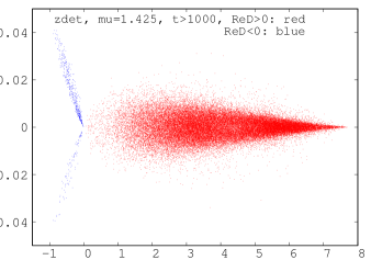
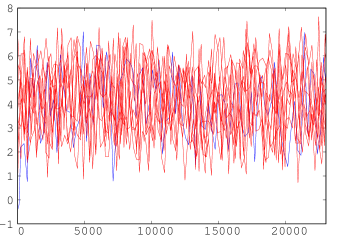
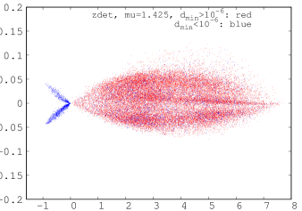
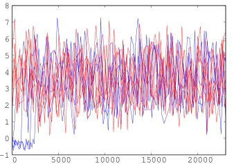
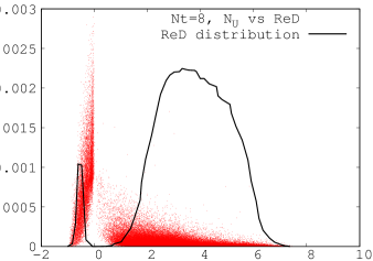
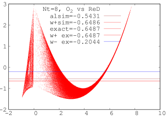
Figure 1: One link effective model, $N_{\tau}=8,\,\kappa=0.12$, $\mu=1.425$ (“bad” point). Top: scatter plot of $D$ and trajectory histories for the ordered case. Middle: same for the disordered case. Bottom: histogram of $\hbox{Re}D$ and correlation of ${\cal N}_{U}$ and $\hbox{Re}D$ (left plot) and of the observable $O_{2}$ and $\hbox{Re}D$ (right plot). See also the text.

The scatter plots for $D$ show a peculiar structure in the “bad" interval (absent outside of it). Here the process also samples two exceptional regions (blue in the upper plots of Fig. 1) characterized by $\hbox{Re}D<0$. They contribute wrong values for the observables. They are connected by a bottleneck at $D=0$ to the “red" region, therefore $\hbox{Re}D<0$ contributions come from trajectories which went near $D=0$. Trajectories starting in “blue" typically switch to “red" and only rarely visit “blue” again.

From the relative weight of the “blue" regions one estimates a systematic error of about $1/1000$, in agreement with observed deviations - see the histogram on left bottom plot of Fig. 1. Discarding the “blue” contributions leads to good results in the ordered case, see Fig. 1 right bottom plot comparing the simulation and the exact results from all and from the “red”/“blue” ($w^{\pm}$) regions. See Fig. 2 for an extended comparison in the ordered case (the agreement is less good in the disordered case).

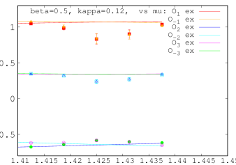
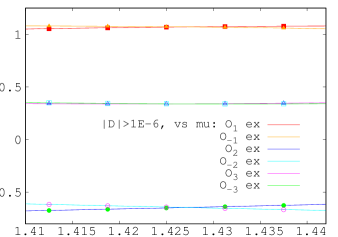
Figure 2: One link model, $N_{\tau}=8,\,\kappa_{N_{\tau}}=0.12$: Observables vs $\mu$ from all regions and from the “red” region.

4 From simple models to QCD

4.1 The Polyakov chain model

A Polyakov chain of $N_{\tau}$ links allows to test procedures involving full gauge field integration of many links Seiler:2012wz . Since it can be reduced by gauge transformations to the one link model of Sec. 3 one can compare with exact results. On the other hand, the direct integration in the full group space over the $N_{\tau}$ links allows to see the effects of accumulation of round-off errors, cooling, etc. This model is a step toward HD-QCD which is no longer exactly solvable.

We shall consider two versions, referred to as model 1 and model 2 below:

$$1:\ -S_{1} = \beta(P+{\tilde{P}})+2n_{f}\ln(1+aP+b{\tilde{P}}),\quad 2:\ -S_{2}=(\beta+2n_{f}a)P+(\beta+2n_{f}b){\tilde{P}},$$ (6)

$$P = \hbox{tr}\prod_{t=1}^{N_{\tau}}U_{t},\quad\quad{\tilde{P}}=\hbox{tr}\left(\prod_{t=1}^{N_{\tau}}U_{t}\right)^{-1}$$ (7)

with $a,\,b$ of Sec. 3 and $n_{f}$ the number of flavours. CL proceeds in the group algebra:

$$U^{\prime}_{t}=\exp\left(-\sum_{a}\hbox{i}\,\lambda^{a}(\epsilon D^{a}_{t}S[U]+\sqrt{\epsilon}\eta_{t}^{a})\right)U_{t}$$ (8)

with $D^{a}$: covariant derivative. Model 1 is the direct extension of that in Sec. 3, model 2 is the un-resummed version of model 1 Stamatescu:2016dwx and has no zeroes. We test two “cooling" methods to control the drift in the noncompact direction by minimising:

$${\rm I:}\quad{\cal N}_{U}=\sum_{t}(\hbox{tr}(U_{t}\,U_{t}^{\dagger})-3),\quad\quad\quad{\rm II:}\quad{\cal N}_{I}=\sum_{t}\sum_{a}\left(\hbox{Im}D^{a}_{t}S[U]\right)^{2}$$ (9)

This proceeds by non-compact gauge transformations using the covariant gradients of the norms. In Table 1 we show typical results for $\beta=0.5,\,N_{\tau}=8,\,\kappa=0.12,\,\mu=1.4,\,\epsilon=10^{-5}$(non-adaptive). We cool after each updating step: one sweep Cooling I (1 0), one sweep Cooling II (0 1), or  both (1 1).
The best results are obtained with more cooling sweeps. Remarks:
- It appears important to start in or near the $SU(3)$ manifold and to cool during thermalisation;
- The value of ${\cal N}_{U}$ can vary (if it stays below $\leavevmode\nobreak\ 0.1$), especially with (1,1) cooling;
- For model 1 cooling also seems to improve concerning the effects of the non-holomorphy.

Table 1: Comparing cooling types for the Polyakov chain model. The statistical errors are $O(10^{-3})$.

$P$ exact:	model 1:	$P_{full}=1.2775$	$(ph.q.:1.2873)$		model 2:	$P_{full}=1.5637$	$(ph.q.:1.5822)$
cooling	${\cal N}_{U}$	${\cal N}_{I}$	$P$		${\cal N}_{U}$	${\cal N}_{I}$	$P$
1 0	$0.56\,10^{-4}$	$0.17\,10^{-5}$	$1.2773$		$0.22\,10^{-2}$	$0.89\,10^{-5}$	$1.5676$
0 1	$0.89\,10^{-3}$	$0.15\,10^{-5}$	$1.2800$		$0.13\,10^{-1}$	$0.95\,10^{-5}$	$1.5658$
1 1	$0.48\,10^{-4}$	$0.10\,10^{-5}$	$1.2734$		$0.21\,10^{-2}$	$0.85\,10^{-5}$	$1.5695$

4.2 HD-QCD

HD-QCD arises in the limit $\kappa\rightarrow 0,\ \mu\rightarrow\infty$ where the determinant of QCD becomes a product of factors Eq. (4) over all Polyakov loops Bender:1992gn . Calculations have explored among other things the phase diagram of the model , see e.g. DePietri:2007ak (reweighting), Aarts:2016qrv (CL).

As before, the correctness of the results depends on the weight of the $\hbox{Re}D<0$ regions, which was there typically $O(10^{-2}-10^{-4})$ and we found a corresponding systematic error of the same magnitude. Now this weight and the associated systematic error are difficult to estimate, due to the superposition of single regions in the product of factors which define the determinant. We therefore need direct simulations and tests. Comparing CLE and reweighting in the region where the latter is reliable ($\mu<1$ with phase rewighting) DePietri:2007ak we have observed generally good agreement but increasing deviations for $\beta\leq 5.7$ Seiler:2012wz . Lower temperatures require therefore large $N_{\tau}$ which would permit to work at large $\beta$. This appears to be a question of computer power but further tests may be necessary.

4.3 Full QCD in the $\kappa$ expansion

Splitting the fermionic determinant into temporal and spatial contributions we evaluate the first factor analytically (HD-QCD) and use a hopping expansion for the spatial part Aarts:2014bwa , Fromm:2011qi . This was shown to converge towards full QCD at sensible parameter choices already around order ten Aarts:2014bwa .

As we have learned from HD-QCD we need $\beta>5.7$ for the gauge cooling to be effective. Here we stay with $\beta=6$. We present for illustration preliminary $O(\kappa^{10})$ results on lattices of $10^{3}\times N_{\tau}$ at $\beta=6,\,\kappa=0.12$, aimed at the phase diagram of QCD. For an investigative study trying to reach low temperatures we use large $N_{\tau}$ but are aware of the finite size effects induced by the wrong aspect ratio.

In the upper two plots of Fig. 3 we fix a rather low temperature $N_{\tau}=16$ and vary $\mu$. It appears that we can explore both the confining and the deconfining phase. At $\mu=0$ the gauge cooling ensures that the results agree with those obtained by reunitarisation, which is equivalent to a real Langevin simulation (blue and green dots at $\mu=0$ on the plots). Notice that the agreement may be lost by choosing an inadequate $\beta<6$ where cooling becomes ineffective Bloch:2017jzi , Sinclair:2016nbg .

In the lower two plots of Fig. 3 we vary the temperature $T=1/N_{\tau}$ by increasing $N_{\tau}$ at fixed $\mu$. Starting at high temperature in the deconfining phase for $\mu\leq 1.1$ we see the signal of the transition to the confining phase at $T\sim 0.1$ ($N_{\tau}\simeq 10$), especially perspicuous in the Polyakov loops. At $\mu\geq 1.8$ we see fully saturated density at low temperature and slightly decreasing at higher $T$.

In the region $0\leq\mu\leq 1.1$ cooling is effective and we observe the silver blaze phenomenon expected in the confining region already at $N_{\tau}=16$. Likewise the region of $\mu\geq 1.8$ is accessible and shows the expected saturation effects. We also see from both sides the signal of approaching a transition, but we could not enter the region $1.1<\mu<1.8$ in order to resolve it with only standard gauge cooling. For the further developments we might be forced to resort to further procedures such as dynamical stabilisation Attanasio:2016mhc and other improvements, Schmalzbauer:2016pbg . This is work in progress. See also Sexty:2013ica .

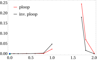
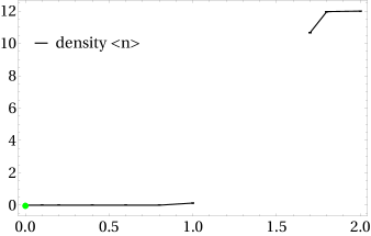
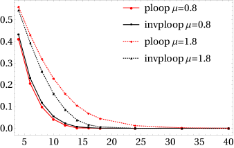
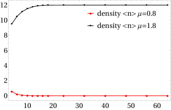
Figure 3: QCD in $\kappa$ expansion, $\beta=6,\kappa=0.12$. Top: $\mu$-dependence of the Polyakov loop (left) and of the density (right) at fixed $N_{\tau}=16$. Bottom: $N_{\tau}$-dependence of the Polyakov loop (left) and of the density at fixed $\mu$ (right).

5 Further prospects: $SU(2)$ real time simulations

Revisiting direct simulations of the Minkowski action in $SU(2)$ Berges:2007nr , Berges:2006xc , the use of gauge cooling Seiler:2012wz and dynamical stabilisation Attanasio:2016mhc show promising improvements. Various integration contours are possible Berges:2006xc , Alexandru:2016gsd , we found as optimal an isosceles triangle with base of extension $\tau$ along the imaginary axis and of extension $t_{0}$ in the real time direction, discretised in $N_{t}$ points.

The left plot of Fig. 4 depicts the maximum possible real time extent $t_{0}$ of the contour for fixed $\tau=16$ and $N_{t}=16$. Here gauge fixing fails but gauge cooling and dynamical stabilisation allow for a non-zero real-time extent in an interesting $\beta$-region. Note that for small $N_{t}$ there can be deviations in the expectation value of the spatial plaquette between the euclidean and the real-time contour. This difference however becomes smaller as one increases $N_{t}$. The right plot depicts the difference as a function of $N_{t}$ at fixed $t_{0}$. . The discretisation of $t_{0}$, $N_{t}$, is relevant. Larger $\beta$ allow larger real time extents. The maximum extent of $t_{0}$ strongly depends on $\tau$. For smaller $\tau$ larger ratios $t_{0}/\tau$ are possible.

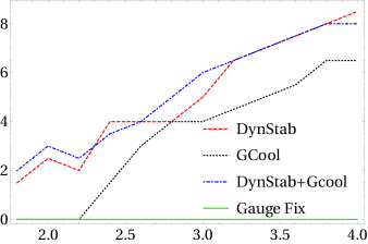
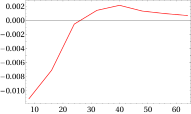
Figure 4: $SU(2)$ real time evolution. Left Maximal possible real time extent $t_{0}$ vs. $\beta$ for $N_{s}=8$, $N_{t}=16$ and inverse temperature $\tau=16$. Right: Difference of the spatial plaquette between the euclidean and the symmetric triangle contour with real time extent $t_{0}=3$ as a function of $N_{t}$ at $\beta=3$, $N_{s}=16$.

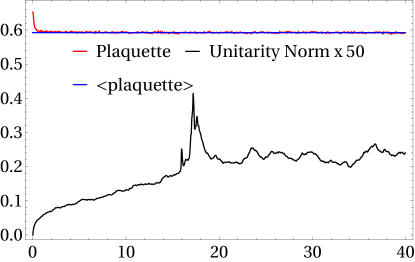
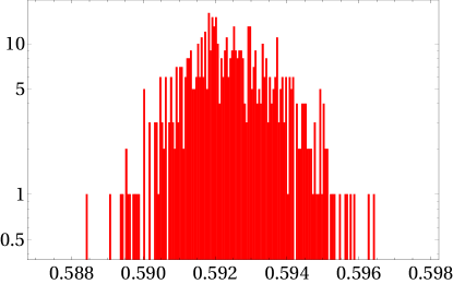
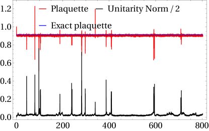
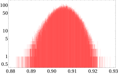
Figure 5: Cooling effectiveness. Top: QCD in $\kappa$ expansion, $\beta=6,\,\kappa=0.12,\,N_{\tau}=16$,   Langevin evolution with cooling (12 sweeps per dynamical sweep) of ${\cal N}_{U}$ and the plaquette (left) and histogram of the latter using the regions of bounded ${\cal N}_{U}$ (right). Bottom: $SU(2)$ real time on the isoscel triangle, $N_{s}=4$, $N_{t}=8$, $\beta=16$,  Langevin evolution with cooling (2 sweeps) of the unitarity norm and the spatial plaquette (left) and histogram of the plaquette using ${\cal N}_{U}<0.07$ (right). Before discarding the peaks in ${\cal N}_{U}$ the histograms had pronounced skirts.

6 Conclusions

Gauge cooling Seiler:2012wz (and its further developments) appear essential for controlling the behaviour of the CL distributions both in the far non-compact direction and near the poles Aarts:2017vrv , see also review . The efficiency of the CL method for lattice gauge theories therefore strongly depends on the effectiveness of cooling. The latter can be judged from the unitarity norm ${\cal N}_{U}$ which is expected to stabilise at some value fixed by the dynamics. In the simulation numerical errors may eventually lead to a divergence of ${\cal N}_{U}$, but as long as ${\cal N}_{U}$ stays bounded we can sample reliable results.

The evolution of the ${\cal N}_{U}$ under cooling permits to judge the efficiency of the latter and therefore the reliability of the results - see Fig. 5. Isolated peaks do not spoil the simulation as long as there are sufficiently long intervals of small unitarity norm. Removing the occasional peaks and selecting the intervals of small ${\cal N}_{U}$ leads then to well behaved distributions and correct convergence of the simulation (remember that cooling is a gauge transformation). For tests of other cooling procedures see, e.g. Nagata:2016vkn , Nagata:2016mmh , Attanasio:2016mhc .

For QCD lattice calculations at $\mu>0$ our results in a 10-th order $\kappa$ expansion show that simulations in the confinement and deconfining phases are possible for $\beta$ large enough. Work in progress concerns resolving the phase transition region. Low temperatures require large lattices in order to ensure a good aspect ratio. A lesson from the study of simple models is to check the appearence of domains with $\hbox{Re}D<0$, drop their contributions and estimate a possible systematic error. As shown in Aarts:2017vrv the signal is already visible in the observables and can thus be easily monitored.

For SU(2) real time evolution cooling and dynamical stabilisation are shown to improve the simulations also for smaller $\beta$, future work is however still necessary to achieve realistic scenarios.

References

- (1) G. Aarts, L. Bongiovanni, E. Seiler, D. Sexty, I.-O. Stamatescu, Eur. Phys. J. A 49 (2013) 89 [arXiv:1303.6425 [hep-lat]]
- (2) E. Seiler, these proceedings.
- (3) G. Aarts, E. Seiler and I. O. Stamatescu, Phys. Rev. D 81 (2010) 054508 [arXiv:0912.3360 [hep-lat]].
- (4) G. Aarts, F. A. James, E. Seiler and I. O. Stamatescu, Eur. Phys. J. C 71 (2011) 1756 [arXiv:1101.3270 [hep-lat]].
- (5) G. Aarts, E. Seiler, D. Sexty and I.-O. Stamatescu, JHEP 1705 (2017) 044 [arXiv:1701.02322 [hep-lat]].
- (6) G. Aarts, F. A. James, J. M. Pawlowski, E. Seiler, D. Sexty and I.-O. Stamatescu, JHEP 03 (2013) 073, [arxiv: 1212.5231 [hep-lat]].
- (7) E. Seiler, D. Sexty and I.-O. Stamatescu, Phys. Lett. B 723 (2013) 213, [arXiv:1211.3709 [hep-lat]].
- (8) K. Nagata, J. Nishimura and S. Shimasaki, Phys. Rev. D 94 (2016) no.11, 114515 [arXiv:1606.07627 [hep-lat]].
- (9) K. Nagata, H. Matsufuru, J. Nishimura and S. Shimasaki, PoS LATTICE 2016 (2016) 067 [arXiv:1611.08077 [hep-lat]].
- (10) F. Attanasio and B. Jäger, PoS LATTICE2016 (2016) 053, [arxiv:1610.09298[hep-lat]].
- (11) I.-O. Stamatescu and E. Seiler, PoS LATTICE 2016, 357 (2016) [arXiv:1611.00620 [hep-lat]].
- (12) I. Bender, T. Hashimoto, F. Karsch, V. Linke, A. Nakamura, M. Plewnia, I.-O. Stamatescu and W. Wetzel, Nucl. Phys. Proc. Suppl. 26, 323 (1992).
- (13) R. De Pietri, A. Feo, E. Seiler and I.-O. Stamatescu, Phys. Rev. D 76 (2007) 114501 [arXiv:0705.3420 [hep-lat]].
- (14) G. Aarts, F. Attanasio, B. JÃger and D. Sexty, JHEP 1609 (2016) 087 [arXiv:1606.05561 [hep-lat]].
- (15) G. Aarts, E. Seiler, D. Sexty and I.-O. Stamatescu, Phys. Rev. D 90, 114505 (2014), [arXiv:1408.3770 [hep-lat]].
- (16) M. Fromm, J. Langelage, S. Lottini and O. Philipsen, JHEP 1201 (2012) 042 [arXiv:1111.4953 [hep-lat]].
- (17) J. Bloch and O. Schenk, [arXiv:1707.08874 [hep-lat]].
- (18) D. K. Sinclair and J. B. Kogut, PoS LATTICE 2016, 026 (2016), [arXiv:1611.02312 [hep-lat]].
- (19) S. Schmalzbauer and J. Bloch, PoS LATTICE 2016 (2016) 362 [arXiv:1611.00702 [hep-lat]].
- (20) D. Sexty, Phys. Lett. B 729 (2014) 108 [arXiv:1307.7748 [hep-lat]].
- (21) J. Berges and D. Sexty, Nucl. Phys. B 799 (2008) 306 [arXiv:0708.0779 [hep-lat]].
- (22) J. Berges, S. Borsanyi, D. Sexty and I.-O. Stamatescu, Phys. Rev. D 75 (2007) 045007 [hep-lat/0609058].
- (23) A. Alexandru, G. Basar, P. F. Bedaque, S. Vartak and N. C. Warrington, Phys. Rev. Lett. 117 (2016) 081602 [arXiv:1605.08040 [hep-lat]].
- (24)