Optimal lattice configurations for interacting spatially extended particles

Abstract

We investigate lattice energies for radially symmetric, spatially extended particles interacting via a radial potential and arranged on the sites of a two-dimensional Bravais lattice. We show the global minimality of the triangular lattice among Bravais lattices of fixed density in two cases: In the first case, the distribution of mass is sufficiently concentrated around the lattice points, and the mass concentration depends on the density we have fixed. In the second case, both interacting potential and density of the distribution of mass are described by completely monotone functions in which case the optimality holds at any fixed density.

AMS Classification: Primary 74G65; Secondary 82B20.
Keywords: Calculus of variations; Lattice energy; Triangular lattice; Crystal.

1 Introduction and main results

One key objective in crystallization theory is to understand the optimal arrangement of particles, interacting with some nonlocal interaction potential. In particular, it has been shown that the triangular lattice is optimal among Bravais lattices for a large class of interaction potentials if one assumes that the particles are located on the lattice sites [35, 37, 2, 40, 16, 11, 6]. The idea of this paper is to generalize these results by considering the optimal arrangement for particles which are not necessarily concentrated on a single point, but may be spatially extended. We note that the question for optimal arrangement of diffuse particles appears naturally in various systems in condensed matter theory [29] and quantum physics, including e.g. Thomas-Fermi model [12] (where the electron density plays the role of the diffuse particle), diblock copolymer systems in the low volume fraction limit [38] and magnetized disks interactions [27]. For related mathematical analysis for these systems, we refer refer e.g. to [11, 17, 18, 30]. We also note that systems with localizing and delocalizing interactions, although in a dynamic setting, are also relevant in biological models related to swarming and flocking, see e.g. [4, 46, 3, 14] and the references therein. We show that for particles with radially symmetric mass distribution, the triangular lattice is still optimal if the mass of each particle is either sufficiently concentrated near its center, or if the mass distribution is described by a completely monotone function.

We consider a collection of identical particles with center located on the sites of a two-dimensional Bravais lattice $L\subset\mathbb{R}^{2}$. The mass distribution of the particle at the lattice site $x\in L$ is given by $\mu(\cdot-x)$ for some given probability measure $\mu\in{\mathcal{P}}(\mathbb{R}^{2})$. Summing the interaction energy between different particles over all the lattice sites, we arrive at the total energy per particle of the lattice:

Definition 1 (Lattice Energy).

For any Bravais lattice $L\subset\mathbb{R}^{2}$ and $\mu\in{\mathcal{P}}(\mathbb{R}^{2})$ , we define the interaction energy ${\mathcal{E}}_{f,\mu}[L]$ by

$${\mathcal{E}}_{f,\mu}[L]:=\sum_{x\in L}{\vphantom{\sum}}^{\prime}\int\!\!\!\!\int_{\mathbb{R}^{2}\times\mathbb{R}^{2}}f(u-x-v)d\mu(u)d\mu(v)\quad\in[0,\infty].$$ (1.1)

The interaction potential $f:\mathbb{R}^{2}\to\mathbb{R}$ is assumed to be in the class ${\mathcal{F}}$, defined as the set of functions $f:\mathbb{R}^{2}\to\mathbb{R}$ such that there exists $C>0$ and $\eta>0$ such that $|f(x)|+|\hat{f}(x)|\leq\frac{C}{(1+|x|)^{2+\eta}}$ for any $x\in\mathbb{R}^{2}$ and such that for some nonnegative Radon measure $\mu_{f}$, we have

$$f(x)=\int_{0}^{\infty}e^{-|x|^{2}t}d\mu_{f}(t) \text{for any $x\in\mathbb{R}^{2}$}.$$ (1.2)

Here and in the sequel, we use the notation $\sum_{x\in L}{\vphantom{\sum}}^{\prime}:=\sum_{x\in L\backslash\{0\}}$. The Fourier transform $\hat{f}$ is defined in (1.9). We also note that the condition (1.2) is equivalent to the fact that $F:(0,\infty)\to\mathbb{R}$, given by $F(|x|^{2}):=f(x)$ is completely monotone, i.e. $(-1)^{k}\partial^{k}F(r)\geq 0$ for all $k\in\mathbb{N}$ and $r>0$. In particular, standard potentials such as the Gaussian potential $g_{\alpha}(x):=e^{-\alpha|x|^{2}}$, $\alpha>0$ and $f_{a}(x)=(a+|x|^{2})^{-s}$, $a>0$, $s>1$, are included into the class of considered potentials (see also [6, Sec. 2.3] and [34]). We note that the energy can be in general infinite since the measure is not assumed to be absolutely continuous.

In previous contributions, most results have been concerned with the case when the particles are located on a single point, i.e. when $\mu$ is given by a Dirac distribution. In this case, the optimality of the triangular lattice

$$\Lambda:=\sqrt{\tfrac{2}{\sqrt{3}}}\left[\mathbb{Z}\left(1,0\right)\oplus\mathbb{Z}\left(\tfrac{1}{2},\tfrac{\sqrt{3}}{2}\right)\right],$$ (1.3)

among the class of Bravais lattices with prescribed density has been established for various interaction potentials, including the class ${\mathcal{F}}$. One key result is the seminal paper by Montgomery [35] where the optimality of the triangular lattice is shown for a class of Gaussian interaction potentials in which case the lattice energy is described by the lattice theta function $\theta_{L}$ given by (2.10). Furthermore, the proof of the minimality of the triangular lattice for a class of Riesz potentials has been established in a series of papers from number theorists [39, 15, 25, 24] in their analysis of the Epstein zeta function. Montgomery result for the lattice theta function was used in order to prove the optimality of a triangular lattice in several physical systems such as Ginzburg-Landau vortices or Bose-Einstein Condensates in the periodic case [37, 2, 36, 40, 10]. In [11, 6, 5, 9, 7], the first author has studied this minimization problem among Bravais lattices for more general potentials $f$. As explained in [13, Sect. 2.5], the minimization of energies per point among Bravais lattices is related to the crystallization conjecture, once the crystallization – i.e. the periodicity of the ground state for this system of interacting (extended) particles – is assumed. Furthermore, even though this conjecture has not been proved so far, some interesting advances have been achieved in the last decade for general configurations of particles in dimension $d\in\{2,3\}$ (we refer e.g. to [45, 26, 43, 44, 32, 33, 31]).

In our first result, we consider particles which are described by radially symmetric mass distributions $\mu\in{\mathcal{P}}(\mathbb{R}^{2})$. Moreover, we define in Section 2.1 a metric on the space of Bravais lattices with unit density. The open ball of radius $R$ and centred at $L$ is then denoted by $B_{R}(L)$. We show that the triangular lattice is energetically optimal if the particles are sufficiently concentrated:

Theorem 2 (Radially symmetric mass distribution).

Let $f\in{\mathcal{F}}$, $\mu\in{\mathcal{P}}(\mathbb{R}^{2})$ be rotationally symmetric with respect to the origin and $\mu_{\epsilon}$ for any measurable set $F\subset\mathbb{R}^{2}$ be given by

$$\mu_{\epsilon}(F):=\mu(\epsilon F).$$ (1.4)

Furthermore, suppose that ${\mathcal{E}}_{f,\mu_{\epsilon}}[L]<\infty$ for any $L\in B_{c}(\Lambda)$, for some $c>0$, and for all sufficiently small $\epsilon$, where the triangular lattice $\Lambda$ is defined by (1.3). Then there exists $\epsilon_{0}=\epsilon_{0}(f,\mu)$ such that for any $0\leq\epsilon<\epsilon_{0}$, $\Lambda$ is the unique minimizer, up to rotation, of ${\mathcal{E}}_{f,\mu_{\epsilon}}$ among all Bravais lattices of unit density.

Our next result shows that if the mass distribution of each particle can be expressed by a completely monotone function in terms of the square root of the radius, then the triangular lattice is again the global minimizer:

Theorem 3 (Completely monotone mass distribution).

Let $f\in{\mathcal{F}}$ and suppose that $\mu\in{\mathcal{P}}(\mathbb{R}^{2})$ satisfies $d\mu(x)=\rho(x)dx$ for some $\rho:\mathbb{R}^{2}\to\mathbb{R}$ satisfying

$$\rho(x)=\int_{0}^{\infty}e^{-|x|^{2}t}d\mu_{\rho}(t) \text{for any $x\in\mathbb{R}^{2}$},$$ (1.5)

for some nonnegative Radon measure $\mu_{\rho}$. Then the triangular lattice $\Lambda$ is the unique minimizer, up to rotation, of ${\mathcal{E}}_{f,\mu}$ among all Bravais lattices of unit density.

The argument for Theorem 2 is based on a perturbation argument and the local optimality of the triangular lattice for $\epsilon$ sufficiently small. The proof of Theorem 2 is given in Section 2.2. The proof of Theorem 3, given in Section 2.3, is a generalization of the arguments used in the proof of the optimality of the triangular lattice for point masses. In particular, the argument is based on the fact that the triangular lattice is self-dual and that the class of completely monotone functions is stable with respect to multiplication. Some of the tools in [11, 6, 5] will be used in order to prove our results as well as computations from [41, 23]. We note that if $\mu$ satisfies the condition of Theorem 3, then for any $\epsilon>0$, the density $\mu_{\epsilon}$ defined by (1.4) also satisfies these conditions. In this sense, the result of Theorem 3 is independent of the concentration of the particles, while this is not the case for Theorem 2.

The paper is concerned with the case of absolutely summable interaction potentials in two dimensions. However, we believe that these results can be generalized. In particular, the results should still hold true for non–integrable interaction potentials such as the Riesz potentials $f(x)=|x|^{-s}$ for any $s>0$ if a cut-off argument near the origin is applied and the Ewald summation method is used to obtain summability for large $x$ in the non-summable case (see for instance [28, Section IV]). Moreover, as explained in Remark 13, all our results related to local minimality could be written in dimensions $4,8$ and $24$ where the densest packing is self-dual, and is expected to be the unique minimizer of the theta function for any $\alpha>0$. In these dimensions, only local minimality results have been proved [41, 23], but some recent results [47, 21] have opened the door for a proof of this universality in dimension $8$ and $24$, and then to a generalization of our result in those dimensions (see also Remark 13). Another interesting question would be to consider the Lennard-Jones-type potentials of the form $f(x)=a_{1}|x|^{-p}-a_{2}|x|^{-q}$, $p>q$, which is widely used in molecular simulation (see [6, Section 6.3] for some examples). In this situations, the generalization of our results should hold under the additional assumption that the density of the lattice is sufficiently high (see [11, 6] for the optimality of the triangular lattice in the point mass case for Lennard-Jones-type potentials). Another interesting extension would be to allow for signed measures or to consider lattice configurations with alternating charges as in [8].

Notation.

We recall (see e.g. [39, 35, 5]) that a two-dimensional Bravais lattice $L\subset\mathbb{R}^{2}$ is a set of the form $L=\mathbb{Z}u_{1}\oplus\mathbb{Z}u_{2}$ for two linearly independent vectors $u_{1}$, $u_{2}\in\mathbb{R}^{2}$. The dual lattice $L^{*}$ is given by $L^{*}$ $=\{p\in\mathbb{R}^{2}\$: $\ p\cdot x\in\mathbb{Z}\text{ for all $x\in L$}\}$. Up to isometry, any Bravais lattice $L\subset\mathbb{R}^{2}$ of unit density can be written as

$$L:=\overline{L}(x,y):=\mathbb{Z}\left(\frac{1}{\sqrt{y}},0\right)\oplus\mathbb{Z}\left(\frac{x}{\sqrt{y}},\sqrt{y}\right) (x,y)\in D$$ with , (1.6)

where $(x,y)\in D$ are uniquely determined in the fundamental domain $D$ with

$$D:=\left\{(x,y)\in\big{[}0,\tfrac{1}{2}\big{]}\times(0,\infty):x^{2}+y^{2}\geq 1\right\}.$$ (1.7)

The set ${\mathcal{D}}$ is the set of lattices of the form (1.6). It is hence sufficient to restrict our analysis to the set of lattices in ${\mathcal{D}}$. Finally, by ${\mathcal{P}}(\mathbb{R}^{2})$ we denote the space of probability measures. The Laplace transform of a Radon measure $\mu$ on $(0,\infty)$ is

$$({\mathcal{L}}\mu)(r):=\int_{0}^{\infty}e^{-rt}d\mu(t).$$ (1.8)

The Fourier transform $\hat{f}:\mathbb{R}^{2}\to\mathbb{C}$ is denoted by

$$\widehat{f}(p):=\int_{\mathbb{R}^{2}}f(x)e^{-2i\pi p\cdot x}dx.$$ (1.9)

2 Proofs

2.1 Preliminaries

We will work with Bravais lattices of the form (1.6). To get a notion of local minimality, we introduce a topology and define the distance of two lattices by

$$d(L_{1},L_{2})=\sqrt{\inf_{k\in\mathbb{Z}}|x_{1}-x_{2}-\tfrac{1}{2}k|^{2}+|y_{1}-y_{2}|^{2}} \text{for $L_{i}=\overline{L}(x_{i},y_{i})\in{\mathcal{D}}$}.$$ (2.1)

We also denote by $B_{R}(L)$ the set of all $\tilde{L}\in{\mathcal{D}}$ with $d(L,\tilde{L})<R$. We write $f\in C^{k}({\mathcal{D}})$ if $f$ is $k$-times differentiable in $(x,y)$. As usual we denote the gradient by $\nabla E[L]:=(\partial_{x}E,\partial_{y}E)[L]$. The Hessian $D^{2}E$ is defined as the matrix of second derivatives w.r.t. $x$, $y$. $D^{3}E$ is correspondingly the tensor of all third derivatives. We also define:

Definition 4 (Local minimizers and critical points in ${\mathcal{D}}$).

Let $E:{\mathcal{D}}\to\mathbb{R}$. $L$ is a strict local minimizer in ${\mathcal{D}}$ if there is $\eta>0$ such that $E[L]<E[\tilde{L}]$ for all $\tilde{L}\in B_{\eta}(L)$. Furthermore, $L$ is a critical point of $E\in C^{1}({\mathcal{D}})$ in ${\mathcal{D}}$ if $\nabla E[L]=(0,0)$.

Before we consider the case of diffuse charge configurations, we collect some basic facts about the interaction energy for point charges:

Definition 5 (Sharp interface energy).

For $h\in{\mathcal{F}}$ and $L\in{\mathcal{D}}$, we define

$$E_{h}[L]:=\sum_{p\in L}{\vphantom{\sum}}^{\prime}h(p).$$ (2.2)

We turn to the investigation of local minimality of lattice energies for spread out particles. We first recall the summation formula of Poisson [42, Cor. 2.6]:

Proposition 6 (Poisson summation formula).

For $f\in{\mathcal{F}}$ and $L\in{\mathcal{D}}$, we have

$$\sum_{x\in L}f(x+z)=\sum_{p\in L^{*}}e^{2\pi ip\cdot z}\hat{f}(p) z\in\mathbb{R}^{2}$$ for all , (2.3)

and the series on both sides of (2.3) converge absolutely.

We note that the assumption in Definition 1 on the decay of $f$ and $\hat{f}$ is included to ensure that (2.3) can be applied and to get absolute convergence.

A representation of the energy in terms of Fourier variables is given next:

Proposition 7 (Fourier representation of ${\mathcal{E}}_{f,\mu}$).

Let $f\in{\mathcal{F}}$, $\mu\in{\mathcal{P}}(\mathbb{R}^{2})$ be rotationally symmetric with respect to the origin and $L\in{\mathcal{D}}$ be such that ${\mathcal{E}}_{f,\mu}[L]<\infty$. Then

$${\mathcal{E}}_{f,\mu}[L]=E_{h}[L^{*}]+\hat{f}(0)-(f\ast\mu\ast\mu)(0)$$ (2.4)

where $E_{h}$ is defined in (2.2) and where

$$\quad h(p):=\hat{f}(p)g(|p|)^{2}, g(t):=\int_{0}^{\infty}J_{0}(2\pi st)d\psi(s).$$ (2.5)

Here, $\psi$ is the Lebesgue–Stieltjes measure of $t\mapsto\mu(B_{t})$, i.e. $\psi([r_{1},r_{2}))=\mu(B_{r_{2}})-\mu(B_{r_{1}})$ and $J_{0}$ is the Bessel function of the first kind.

Proof.

By Fubini and Poisson’s summation formula (Proposition 6), we get

$${\mathcal{E}}_{f,\mu}[L] =\int\!\!\!\!\int_{\mathbb{R}^{2}\times\mathbb{R}^{2}}\sum_{p\in L^{*}}{\vphantom{\sum}}^{\prime}\hat{f}(p)e^{2i\pi p\cdot(u-v)}d\mu(u)d\mu(v)+\hat{f}(0)-(f\ast\mu\ast\mu)(0)$$ (2.6)

$$=\sum_{p\in L^{*}}{\vphantom{\sum}}^{\prime}\hat{f}(p)\Big{(}\int_{\mathbb{R}^{2}}e^{2i\pi p\cdot u}d\mu(u)\Big{)}\Big{(}\int_{\mathbb{R}^{2}}e^{-2i\pi p\cdot v}d\mu(v)\Big{)}+\hat{f}(0)-(f\ast\mu\ast\mu)(0)$$ (2.7)

$$=\sum_{p\in L^{*}}{\vphantom{\sum}}^{\prime}\hat{f}(p)\hat{\mu}(p)^{2}+\hat{f}(0)-(f\ast\mu\ast\mu)(0).$$ (2.8)

The proof is completed by noting that $\hat{\mu}$ is given by the Hankel-Stieltjes transform ([22, Section 2]) and hence $\hat{\mu}=g$ where $g$ is given in (2.5). ∎

Since $\Lambda^{*}=\Lambda$ up to rotation, a consequence of Proposition 7 is that proving the (local) minimality of $\Lambda$ for ${\mathcal{E}}_{f,\mu}$ in ${\mathcal{D}}$ is the same as proving it for $E_{h}$. In particular, we can use the following result:

Lemma 8 ([23, 5]).

Let $L=\Lambda$ be the triangular lattice of unit density. Let $f\in L^{1}(\mathbb{R}^{2})\cap C^{2}(\mathbb{R}^{2}\backslash\{0\})$ be rotationally symmetric with respect to the origin and $F$ be given by $F(|x|^{2}):=f(x)$. Then

1. $\Lambda$ is a critical point of $E_{f}$ in ${\mathcal{D}}$.

2. We have $D^{2}E_{f}[\Lambda]=T_{f}\operatorname*{{Id}}_{\mathbb{R}^{2}}$ where $\operatorname*{{Id}}_{\mathbb{R}^{2}}$ is the identity on $\mathbb{R}^{2}$ and

   $$T_{f}:=\frac{4}{\sqrt{3}}\sum_{m,n}{\vphantom{\sum}}^{\prime}n^{2}F^{\prime}\big{(}\tfrac{2}{\sqrt{3}}(m^{2}+mn+n^{2})\big{)}+\frac{4}{3}\sum_{m,n}{\vphantom{\sum}}^{\prime}n^{4}F^{\prime\prime}\big{(}\tfrac{2}{\sqrt{3}}(m^{2}+mn+n^{2})\big{)}.$$ (2.9)

We next give a generalization of [23, Thm. 4.6] for the two-dimensional case.

Proposition 9 (Local optimality of $\Lambda$ for $E_{f}$).

Let $f\in{\mathcal{F}}$. Then $\Lambda$ is a strict local minimum of $E_{f}$ in ${\mathcal{D}}$ with positive second derivative.

Proof.

We first claim that for any $t>0$, the triangular lattice $\Lambda$ is a strict local minimum in ${\mathcal{D}}$ with positive second derivative of the lattice theta function

$$\theta_{L}(t):=\sum_{x\in L}e^{-\pi t|x|^{2}}=E_{G_{t}}[L]+1,$$ (2.10)

where $G_{t}$ is the Gaussian potential $G_{t}(x)=e^{-\pi t|x|^{2}}$. As explained in [23] for dimensions $d\in\{4,8,24\}$, a direct consequence of [41, Eq. (46)] is that $D^{2}\hskip 2.84526ptE_{G_{t}}[\Lambda]$ is positive definite for any $t>0$. Since we can write, by Fubini’s theorem,

$$E_{f}[L]=\int_{0}^{\infty}\left(\theta_{L}(t/\pi)-1\right)d\mu_{f}(t),$$ (2.11)

for any $f\in{\mathcal{F}}$, the same result also holds all $f\in{\mathcal{F}}$. ∎

Finally, it is useful to note that the class of functions ${\mathcal{F}}$ is stable under the application of the Fourier transform:

Lemma 10.

We have $f\in{\mathcal{F}}$ if and only if $\hat{f}\in{\mathcal{F}}$.

Proof.

We need to show that $\hat{f}$ can be written as in (1.2). By definition, for any $f\in{\mathcal{F}}$ there is a nonnegative Radon measure $\mu_{f}$ such that (1.2) holds. By application of the Fourier transform and by Fubini’s theorem, we then have

$$\hat{f}(p) =\int_{0}^{\infty}\left(\int_{\mathbb{R}^{2}}e^{-|x|^{2}t}e^{-2i\pi x\cdot p}dx\right)d\mu_{f}(t)=\int_{0}^{\infty}e^{-\frac{\pi^{2}}{t}|p|^{2}}t^{-1}d\mu_{f}(t).$$ (2.12)

It follows that $\hat{f}$ can be expressed in the form (1.2) with $\mu_{f}$ replaced by some nonnegative Radon measure $\mu_{\hat{f}}$. ∎

The proof of the next result about local minimality of $\Lambda$ for ${\mathcal{E}}_{f,\mu_{\epsilon}}$ and small $\epsilon$ is given in the Appendix:

Proposition 11 (Local minimality of $\Lambda$ for small $\epsilon$).

Let $f\in{\mathcal{F}}$ and $\mu\in{\mathcal{P}}(\mathbb{R}^{2})$ be rotationally symmetric with respect to the origin. With $\mu_{\epsilon}$ given by (1.4), we assume that ${\mathcal{E}}_{f,\mu_{\epsilon}}[L]<\infty$ for any $L\in B_{c}(\Lambda)$, for some $c>0$, and for all sufficiently small $\epsilon$. Then there exists $\epsilon_{1}=\epsilon_{1}(f,\mu)$ and $c_{0}=c_{0}(f,\mu)>0$ (independent of $\epsilon$) such that for any $0\leq\epsilon<\epsilon_{1}$, the triangular lattice $\Lambda$ is a strict local minimizer of ${\mathcal{E}}_{f,\mu_{\epsilon}}$ in the set of lattices $B_{c_{0}}(\Lambda)$.

Proof.

By Proposition 7 and the fact that $\Lambda^{*}=\Lambda$, up to rotation, we need to show that $\Lambda$ is a strict minimizer of $E_{h_{\epsilon}}$, where $h_{\epsilon}(p):=\hat{f}(p)g_{\epsilon}(|p|)^{2}$ and $g_{\epsilon}(r):=g(\epsilon r)$ with $g$ defined in (2.5). We furthermore set $H_{\epsilon}(|x|^{2}):=h_{\epsilon}(x)=\Phi(|x|^{2})G_{\epsilon}(|x|^{2})^{2}$ with $\Phi(|p|^{2}):=\hat{f}(p)$, $G_{\epsilon}(|p|^{2}):=g_{\epsilon}(|p|)$, i.e.

$$G_{\epsilon}(r)=\int_{0}^{\infty}J_{0}(2\pi s\epsilon\sqrt{r})d\psi(s).$$ (2.13)

By Lemma 8 and the fact that $h_{\epsilon}$ is a radial function, $\Lambda$ is a critical point of $E_{h_{\epsilon}}$ in ${\mathcal{D}}$ for any $\epsilon>0$ and a condition for the strict positivity of its Hessian at $L=\Lambda$ is

$$T_{h_{\epsilon}}:=\frac{4}{\sqrt{3}}\sum_{m,n}{\vphantom{\sum}}^{\prime}n^{2}H_{\epsilon}^{\prime}\Big{(}\tfrac{2}{\sqrt{3}}(m^{2}+mn+n^{2})\Big{)}+\frac{4}{3}\sum_{m,n}{\vphantom{\sum}}^{\prime}n^{4}H_{\epsilon}^{\prime\prime}\Big{(}\tfrac{2}{\sqrt{3}}(m^{2}+mn+n^{2})\Big{)}>0.$$ (2.14)

Since $J_{0}^{\prime}(r)=-J_{1}(r)$ and $J_{1}^{\prime}(r)=\frac{1}{2}(J_{0}(r)-J_{2}(r))$, a simple calculation yields

$$(G_{\epsilon}^{2})^{\prime}(r)=-\frac{2\pi\epsilon}{\sqrt{r}}\Big{(}\int_{0}^{\infty}sJ_{1}(\tilde{r})d\psi(s)\Big{)}\Big{(}\int_{0}^{\infty}J_{0}(\tilde{r})d\psi(s)\Big{)},$$ (2.15)

with the notation $\tilde{r}:=2\pi s\epsilon\sqrt{r}$. Furthermore,

$$(G_{\epsilon}^{2})^{\prime\prime}(r)= \frac{\pi\epsilon}{r^{3/2}}\int_{0}^{\infty}J_{0}(\tilde{r})d\psi(s)\int_{0}^{\infty}sJ_{1}(\tilde{r})d\psi(s)+\frac{2\pi^{2}\epsilon^{2}}{r}\Big{(}\int_{0}^{\infty}sJ_{1}(\tilde{r})d\psi(s)\Big{)}^{2}$$ (2.16)

$$+\frac{\pi^{2}\epsilon^{2}}{r}\int_{0}^{\infty}J_{0}(\tilde{r})d\psi(s)\int_{0}^{\infty}s^{2}(J_{2}(\tilde{r})-J_{0}(\tilde{r}))d\psi(s).$$ (2.17)

We also recall the series expansion of Bessel functions (see e.g. [1, Eq. (9.1.10)])

$$J_{0}(\tilde{r})=1+\sum_{m=1}^{\infty}\frac{(-1)^{m}(\frac{\tilde{r}}{2})^{2m}}{(m!)^{2}},J_{1}(\tilde{r})=\sum_{m=1}^{\infty}\frac{(-1)^{m}(\frac{\tilde{r}}{2})^{2m+1}}{m!(m+1)!},J_{2}(\tilde{r})=\sum_{m=1}^{\infty}\frac{(-1)^{m}(\frac{\tilde{r}}{2})^{2m+2}}{m!(m+2)!},$$ (2.18)

where $\tilde{r}=2\pi s\epsilon\sqrt{r}$ as before. Thus, using the Leibniz rule on $H_{\epsilon}^{\prime\prime}=(\Phi G_{\epsilon}^{2})^{\prime\prime}$, since $\int_{0}^{\infty}d\psi(s)=1$ and by substituting the expressions of $J_{n}(2\pi s\epsilon\sqrt{r})$, $n\in\{0,1,2\}$, previously computed and summing on $\Lambda$, we obtain $T_{h_{\epsilon}}=T_{\hat{f}}+R_{\epsilon}$, where $R_{\epsilon}\to 0$ as $\epsilon\to 0$. By Lemma 10 we have $\hat{f}\in{\mathcal{F}}$, and it follows from Proposition 9 that $T_{\hat{f}}>0$. Therefore, there exists $\epsilon_{1}$ such that for any $0\leq\epsilon<\epsilon_{1}$, $T_{h_{\epsilon}}>0$, and $\Lambda$ is a local minimum of $E_{h_{\epsilon}}$ in ${\mathcal{D}}$, for any such $\epsilon$. Moreover, as all the $J_{n}$ are bounded, it is straightforward to prove that for any $L\in B_{c}(\Lambda)$ and any $0\leq\epsilon\leq 1$, we have $|D^{3}{\mathcal{E}}_{h_{\epsilon}}[L]|\leq C$ for some $C$ independent of $\epsilon$. This concludes the proof. ∎

2.2 Proof of Theorem 2

In this section, we give the proof of Theorem 2, related to the case of small $\epsilon$. At the end of the section, we give some remarks about the case of large $\epsilon$.

Before proving Theorem 2, we show in the following result that a minimizer $L_{0}\in{\mathcal{D}}$ of $E_{h_{\epsilon}}$ is necessarily at a bounded distance from $\Lambda$.

Lemma 12.

Let $f\in{\mathcal{F}}$ and $\mu\in{\mathcal{P}}(\mathbb{R}^{2})$ be rotationally symmetric with respect to the origin. Suppose that ${\mathcal{E}}_{f,\mu_{\epsilon}}[L]<\infty$ for any $L\in B_{c}(\Lambda)$, for some $c>0$, and for all $\epsilon<\epsilon_{0}$ and some $\epsilon_{0}>0$ where $\mu_{\epsilon}$ is given by (1.4). Then there exists $c_{1}=c_{1}(f,\mu)>0$ and $\epsilon_{1}=\epsilon_{1}(f,\mu)$ such that for any $0\leq\epsilon<\epsilon_{1}$ and any minimizer $L_{0}$ of $E_{h_{\epsilon}}$ in ${\mathcal{D}}$, we have $L_{0}\in B_{c_{1}}(\Lambda)$.

Proof.

By Proposition 7, it suffices to prove the equivalent statement for the energy

$$E_{h_{\epsilon}}[L]=\sum_{p\in L}{\vphantom{\sum}}^{\prime}h_{\epsilon}(p)=\sum_{p\in L}{\vphantom{\sum}}^{\prime}\Phi(|p|^{2})\int_{0}^{\infty}J_{0}(2\pi s\epsilon|p|)d\psi(s),$$ (2.19)

where $\Phi(|x|^{2})=\hat{f}(x)$ for any $x\in\mathbb{R}^{2}$. Note that $\mu_{\hat{f}}\geq 0$ since $f\in{\mathcal{F}}$ and hence $\hat{f}\in{\mathcal{F}}$ by Lemma 10. We recall that, by definition of ${\mathcal{F}}$ and Lemma 10, $\Phi$ is a completely monotone function – and then decreasing – and $\Phi(|x|^{2})=\hat{f}(x)\leq C(1+|x|)^{-2-\eta}$ for some $\eta>0$. We also note that $\psi([0,\infty))=1$. Let $L=\bar{L}(x,y)\in{\mathcal{D}}$ with $(x,y)\in D$ such that $E_{h_{\epsilon}}[L]<\infty$. Then we have, for any $p=m(\frac{1}{\sqrt{y}},0)+n(\frac{x}{\sqrt{y}},\sqrt{y})\in L$ for some $(m,n)\in\mathbb{Z}^{2}$, $|p|^{2}=\frac{(m+xn)^{2}}{y}+yn^{2}$. We will use that $J_{0}(r)\geq\frac{1}{2}$ for $r\leq 1$ and $J_{0}(r)\geq-\frac{1}{2}$ for $r\geq 1$ (which can be checked easily). Hence, we get, for any $0\leq\epsilon<\epsilon_{0}$,

$$E_{h_{\epsilon}}[L] \geq\frac{1}{2}\sum_{p\in L}{\vphantom{\sum}}^{\prime}\Phi(|p|^{2})\int_{\{s\leq\frac{1}{2\pi\epsilon|p|}\}}d\psi(s)-\frac{1}{2}\sum_{p\in L}{\vphantom{\sum}}^{\prime}\Phi(|p|^{2})\int_{\{s\geq\frac{1}{2\pi\epsilon|p|}\}}d\psi(s)$$ (2.20)

$$\geq\frac{1}{2}\Big{(}I_{1}(\epsilon;L)-I_{2}(\epsilon;L)\Big{)},$$ (2.21)

where for $L=\overline{L}(x,y)$ we write

$$I_{1}(\epsilon;L):=\sum_{p\in L}{\vphantom{\sum}}^{\prime}\Phi(|p|^{2})\psi\Big{(}\{s\leq\frac{1}{2\pi\epsilon|p|}\}\Big{)}, I_{2}(\epsilon;L):=\sum_{p\in L}{\vphantom{\sum}}^{\prime}\Phi(|p|^{2})\psi\Big{(}\{s\geq\frac{1}{2\pi\epsilon|p|}\}\Big{)}.$$ (2.22)

Let $\epsilon_{2}$ be such that $\psi(\{s\leq\frac{1}{2\pi\epsilon_{2}}\})\geq\frac{3}{4}$, and we set $\epsilon_{1}=\min(\epsilon_{2},\epsilon_{0})$. Let $I_{1}=\sum_{p}I_{1}^{p}$ and $I_{2}=\sum_{p}I_{2}^{p}$. We first note that $I_{1}^{p}\geq 0$ and $I_{2}^{p}\geq 0$ for all $p\in L$. Since $\Phi(\frac{1}{z})\to\|f\|_{L^{1}}$ and $\psi(z)\to 1$ for $z\to\infty$, we have $I_{1}(\epsilon;L)\geq I_{1}(\epsilon_{1};L)$ and

$$\liminf_{y\to\infty}I_{1}(\epsilon_{1};L) \geq\sum_{m\in\mathbb{Z}}{\vphantom{\sum}}^{\prime}\liminf_{y\to\infty}\Phi\left(\frac{m^{2}}{y}\right)\psi\Big{(}\{s\leq\frac{\sqrt{y}}{2\pi\epsilon_{1}|m|}\}\Big{)}=\infty,$$ (2.23)

uniformly in $\epsilon$ for all $0\leq\epsilon<\epsilon_{1}$. By definition of $\epsilon_{2}$ we have, for any $0\leq\epsilon<\epsilon_{1}$, $I_{1}^{p}\geq 2I_{2}^{p}$ and hence $I_{1}^{p}-I_{2}^{p}>\frac{1}{2}I_{1}^{p}$ if $|p|\leq 1$. Together with (2.23) this implies that $I_{1}-\sum_{|p|\leq 1}I_{2}^{p}\to\infty$ as $y\to\infty$. It remains to estimate $\sum_{|p|\geq 1}I_{2}^{p}$. We first consider the terms with $n=0$, i.e. $p=(\frac{m}{\sqrt{y}},0)$ with $|p|^{2}=\frac{m^{2}}{y}\geq 1$. Since $\psi\leq 1$, we have for any $y\geq 1$ and any $0\leq\epsilon<\epsilon_{1}$,

$$\sum_{|p|>1,p=(\frac{m}{\sqrt{y}},0)}I_{2}^{p}(\epsilon,L)\leq\sum_{|m|>1,m\in\mathbb{Z}}\Phi(m^{2})\leq\sum_{|m|>1,m\in\mathbb{Z}}\frac{1}{(1+|m|)^{2+\eta}}\leq C.$$ (2.24)

We turn to the estimate of the $n\neq 0$ terms. For any $y\geq 1$, $x\in\left[0,\frac{1}{2}\right]$ and $(m,n)\in\mathbb{Z}\times\mathbb{Z}\backslash\{0\}$ we have $\frac{2xmn}{y}\geq-\frac{x}{y}(m^{2}+n^{2})$, $x^{2}-x\geq-\frac{1}{4}$, $y-\frac{1}{4y}>\frac{y}{2}$ and

$$\frac{(m+xn)^{2}}{y}+yn^{2} \geq\frac{(1-x)m^{2}}{y}+\frac{(x^{2}-x+y^{2})n^{2}}{y}\geq\frac{m^{2}}{2y}+\left(y-\frac{1}{4y}\right)n^{2}$$

$$>\frac{m^{2}}{2y}+\frac{yn^{2}}{2}.$$ (2.25)

Furthermore, we recall that $\Phi$ is decreasing. Therefore, using $\psi\leq 1$ we get, for any $y\geq 1$, any $x\in\left[0,\frac{1}{2}\right]$ and any $0\leq\epsilon<\epsilon_{1}$,

$$\sum_{|p|>1,n\neq 0}I_{2}^{p}(\epsilon,L)\leq\sum_{m,n:n\neq 0}\Phi\Big{(}\frac{(m+xn)^{2}}{y}+yn^{2}\Big{)}\stackrel{{\scriptstyle\eqref{dazuu}}}{{\leq}}\sum_{m,n:n\neq 0}\Phi\Big{(}\frac{1}{2}\Big{(}\frac{m^{2}}{y}+yn^{2}\Big{)}\Big{)}$$ (2.26)

$$\leq C\int\!\!\!\!\int_{\mathbb{R}^{2}}\frac{dudv}{\left(1+\sqrt{\frac{u^{2}}{2y}+\frac{y}{2}v^{2}}\right)^{2+\eta}}=2C\int\!\!\!\!\int_{\mathbb{R}^{2}}\frac{dwdz}{\left(1+\sqrt{w^{2}+z^{2}}\right)^{2+\eta}}<\infty,$$ (2.27)

by the change of variables $w=\frac{u}{\sqrt{2y}}$ and $z=\frac{v\sqrt{y}}{\sqrt{2}}$. We finally obtain that, for any $0\leq\epsilon<\epsilon_{1}$, any $y\geq 1$ and any $0\leq x\leq 1/2$, $E_{h_{\epsilon}}[L]\geq C(y)$ for some function $C$ that depends only on $f,\mu,$ and $\epsilon_{1}$, but is independent of $\epsilon\in[0,\epsilon_{1})$, with $C(y)\to\infty$ for $y\to\infty$. Therefore, there exists $c_{1}>0$ such that $L_{0}\in B_{c_{1}}(\Lambda)$ for such minimizer $L_{0}$. ∎

Proof of Theorem 2.

By Proposition 7, proving the optimality of $\Lambda$ in ${\mathcal{D}}$ for ${\mathcal{E}}_{f,\mu_{\epsilon}}$ is equivalent with proving the same for

$$E_{h_{\epsilon}}[L]=\sum_{p\in L}{\vphantom{\sum}}^{\prime}h_{\epsilon}(p)=\sum_{p\in L}{\vphantom{\sum}}^{\prime}\hat{f}(p)g_{\epsilon}(|p|)^{2},$$ (2.28)

where $g_{\epsilon}(r)=g(\epsilon r)$, $g$ is defined by (2.5) and $h_{\epsilon}(p)=\hat{f}(p)g_{\epsilon}(|p|)^{2}$. We note that in general $H_{\epsilon}$, where $H_{\epsilon}(|p|^{2}):=h_{\epsilon}(p)$, is not completely monotone so that the optimality of the triangular lattice is not clear. However, in the limit $\epsilon\to 0$, $H_{\epsilon}$ approaches the completely monotone function $\Phi$, defined by $\Phi(|x|^{2}):=\hat{f}(x)$. By Lemma 10, there is hence a nonegative Radon measure $\mu_{\hat{f}}$ such that $\Phi={\mathcal{L}}\mu_{\hat{f}}$.

By Lemma 12, if $L_{0}$ is a minimizer of $E_{h_{\epsilon}}$ for small enough $\epsilon$, then $L_{0}\in B_{c_{1}}(\Lambda)$ for some $c_{1}>0$. In the sequel, we will consider only lattices $L\in B_{c_{1}}(\Lambda)$ such that $E_{h_{\epsilon}}[L]<\infty$ (otherwise $L$ is not a minimizer).

We hence approximate $H_{\epsilon}$ by a sequence of completely monotone functions $\tilde{H}_{\epsilon}$. More precisely, we construct $\tilde{H}_{\epsilon}$ such that $E_{\tilde{h}_{\epsilon}}[L]$, defined in (2.2) for $\tilde{h}_{\epsilon}(p):=\tilde{H}_{\epsilon}(|p|^{2})$ satisfies for any $L\in B_{c_{1}}(\Lambda)$

$$\left|E_{\tilde{h}_{\epsilon}}[L]-E_{h_{\epsilon}}[L]\right| \leq C\epsilon^{2} \text{for $\epsilon\to 0$},$$ (2.29)

$$E_{\tilde{h}_{\epsilon}}[L]-E_{\tilde{h}_{\epsilon}}[\Lambda] \geq Cd(L,\Lambda)^{2}.$$ (2.30)

We claim that the assertion of the proposition follows from (2.29)–(2.30). Indeed, if (2.29)–(2.30) hold, then we can estimate for any $L\in B_{c_{1}}(\Lambda)$ ,

$$E_{h_{\epsilon}}[L]-E_{h_{\epsilon}}[\Lambda] =E_{h_{\epsilon}-\tilde{h}_{\epsilon}}[L]+\big{(}E_{\tilde{h}_{\epsilon}}[L]-E_{\tilde{h}_{\epsilon}}[\Lambda]\big{)}-E_{h_{\epsilon}-\tilde{h}_{\epsilon}}[\Lambda]$$ (2.31)

$$\stackrel{{\scriptstyle\eqref{cl-2}}}{{\geq}}Cd(L,\Lambda)^{2}+E_{h_{\epsilon}-\tilde{h}_{\epsilon}}[L]-E_{h_{\epsilon}-\tilde{h}_{\epsilon}}[\Lambda]$$ (2.32)

$$\stackrel{{\scriptstyle\eqref{cl-1}}}{{\geq}}Cd(L,\Lambda)^{2}-2C\epsilon^{2}.$$ (2.33)

For any lattice $L$ with $E_{h_{\epsilon}}[L]\leq E_{h_{\epsilon}}[\Lambda]$, this implies $d(L,\Lambda)\leq C\epsilon$. We claim

$$E_{h_{\epsilon}}[L]\geq E_{h_{\epsilon}}[\Lambda] L\in B_{c_{0}}(\Lambda) 0\leq\epsilon<\epsilon_{0}$$ for all and all , (2.34)

for some $\epsilon_{0}>0$ and some $c_{0}>0$. This follows from Proposition 11. Assuming that (2.34) holds, we get the statement of the theorem.

It remains to show that (2.29)–(2.30) hold. In order to construct $\tilde{H}_{\epsilon}$, we first approximate $g_{\epsilon}^{2}$ by some function $\tilde{g}_{\epsilon}^{2}$. We choose $\tilde{\nu}\in C_{c}^{\infty}((\frac{1}{2},2))$ such that $\tilde{\nu}\geq 0$ and $\int_{0}^{\infty}\tilde{\nu}(t)\ dt=1$. With the definition

$$\tilde{g}(r)^{2}:={\mathcal{L}}\tilde{\nu}(r)=\int_{0}^{\infty}e^{-rt}\tilde{\nu}(t)\ dt$$ (2.35)

and $\tilde{g}_{\epsilon}(r)=\tilde{g}(\epsilon r)$ we then have $\tilde{g}^{2}\in{\mathcal{F}}$, $\tilde{g}(0)^{2}=1$ and $\|(\tilde{g}^{2})^{\prime}\|_{\infty}\leq C$. Since also $\|(g^{2})^{\prime}\|_{\infty}\leq C$ and $g(0)^{2}=1$, we hence get, for any $r>0$,

$$|g_{\epsilon}(r)^{2}-\tilde{g}_{\epsilon}(r)^{2}|=|g(\epsilon r)^{2}-\tilde{g}(\epsilon r)^{2}|\leq C\min\{\epsilon^{2}r,1\}.$$ (2.36)

In terms of $\tilde{\nu}_{\epsilon}(t):=\frac{1}{\epsilon}\tilde{\nu}\big{(}\frac{t}{\epsilon}\big{)}$, we get

$$\tilde{g}_{\epsilon}(r)^{2}=\tilde{g}(\epsilon r)^{2}=\int_{0}^{\infty}e^{-\epsilon rt}\tilde{\nu}(t)\ dt=\int_{0}^{\infty}e^{-rt}\tilde{\nu}_{\epsilon}(t)\ dt.$$ (2.37)

We extend $\tilde{\nu}$ and $\mu_{\tilde{f}}$ by $0$ to measures on $\mathbb{R}$ and define

$$\tilde{\mu}_{\epsilon}(t):=(\mu_{\hat{f}}*\tilde{\nu}_{\epsilon})(t)=\int_{0}^{\infty}\tilde{\nu}_{\epsilon}(t-s)d\mu_{\hat{f}}(s) t>0$$ for . (2.38)

In particular, $\mu_{\hat{f}}\geq 0$. With $u=t-s$ and since $\operatorname*{supp}(\tilde{\nu})\in\left(\frac{1}{2},2\right)$ we calculate

$${\mathcal{L}}\tilde{\mu}_{\epsilon}(r) =\int_{0}^{\infty}\int_{0}^{\infty}e^{-rt}\tilde{\nu}_{\epsilon}(t-s)d\mu_{\hat{f}}(s)dt=\int_{0}^{\infty}\left(\int_{-s}^{\infty}e^{-r(s+u)}\tilde{\nu_{\epsilon}}(u)du\right)d\mu_{\hat{f}}(s)$$ (2.39)

$$=\int_{0}^{\infty}e^{-rs}\left(\int_{0}^{\infty}e^{-ru}\tilde{\nu_{\epsilon}}(u)du\right)d\mu_{\hat{f}}(s)=\tilde{g}_{\epsilon}(r)^{2}\int_{0}^{\infty}e^{-rs}d\mu_{\hat{f}}(s)$$ (2.40)

$$=\Phi(r)\tilde{g}_{\epsilon}(r)^{2}=:\tilde{H}_{\epsilon}(r).$$ (2.41)

In view of (2.36), we then get, for any $p\neq 0$,

$$|H_{\epsilon}(|p|^{2})-\tilde{H}_{\epsilon}(|p|^{2})|=|\hat{f}(p)||g_{\epsilon}(|p|)^{2}-\tilde{g}_{\epsilon}(|p|)^{2}|\leq C|\hat{f}(p)|\min\{\epsilon^{2}|p|,1\}.$$ (2.42)

This implies (2.29) by the dominated convergence theorem since $\hat{f}\in L^{1}(\mathbb{R}^{2})$.

We turn to the proof of (2.30). We note that, since $\tilde{H}_{\epsilon}={\mathcal{L}}\tilde{\mu}_{\epsilon}$,

$$E_{\tilde{h}_{\epsilon}}[L]-E_{\tilde{h}_{\epsilon}}[\Lambda]=\int_{0}^{\infty}\big{[}\theta_{L}(\pi t)-\theta_{\Lambda}(\pi t)\big{]}\tilde{\mu}_{\epsilon}(t)\ dt,$$ (2.43)

where $\theta_{L}$ is the lattice theta function given by (2.10). From the construction, we also have $\tilde{\nu}_{\epsilon}\rightharpoonup\delta_{0}$ and hence $\tilde{\mu}_{\epsilon}=\mu_{\hat{f}}*\tilde{\nu}_{\epsilon}\rightharpoonup\mu_{\hat{f}}$ in the sense of measures for $\epsilon\to 0$. Note that the integrand and the measure are nonnegative by optimality of $\Lambda$ in ${\mathcal{D}}$ for $L\mapsto\theta_{L}(\alpha)$ for any $\alpha>0$ (see [35]) and since $\tilde{\mu}_{\epsilon}\geq 0$. Hence, there is $\delta>0$ (depending on $f$ and $\mu$ but independent of $\epsilon$) such that

$$E_{\tilde{h}_{\epsilon}}[L]-E_{\tilde{h}_{\epsilon}}[\Lambda]\geq\frac{1}{2}\int_{\delta}^{\frac{1}{\delta}}\big{[}\theta_{L}(\pi t)-\theta_{\Lambda}(\pi t)\big{]}d\mu_{\hat{f}}(t).$$ (2.44)

By Proposition 9 and continuity of $(t,L)\mapsto\theta_{L}(\pi t)$, for any $\delta>0$ we have $\theta_{L}(\pi t)-\theta_{\Lambda}(\pi t)\geq cd(L,\Lambda)^{2}$ for all $t\in[\delta,\frac{1}{\delta}]$ and $L\in B_{c_{1}}(\Lambda)$. Then (2.30) follows from the estimate

$$E_{\tilde{h}_{\epsilon}}[L]-E_{\tilde{h}_{\epsilon}}[\Lambda]\geq Cd(L,\Lambda)^{2}\int_{\delta}^{\frac{1}{\delta}}d\mu_{\hat{f}}(t)\geq Cd(L,\Lambda)^{2}.$$ (2.45)

∎

Remark 13 (Higher dimension).

The two important ingredients here are the strict local minimality of $\Lambda$ for $\mathcal{E}_{h_{\epsilon}}$ combined with the global optimality of $\Lambda$ for the theta function $L\mapsto\theta_{L}(\alpha)$ for any $\alpha>0$. The result of Proposition 11 can be easily generalized to dimensions $d\in\{4,8,24\}$, for $D_{4},E_{8}$ and the Leech lattice, using the strict local minimality of these lattices for the $d$-dimensional theta function $L\mapsto\theta_{L}(\alpha)$, for any $\alpha>0$, proved in [23, Thm. 4.6] and the fact that the Fourier transform of a radial measure on $\mathbb{R}^{d}$ is (see e.g. [22, Section 2])

$$\hat{\mu}(p)=\frac{2^{\frac{d}{2}-1}\Gamma\left(\frac{d}{2}\right)}{|p|^{\frac{d}{2}-1}}\int_{0}^{\infty}J_{\frac{d}{2}-1}(2\pi s|p|)s^{1-\frac{d}{2}}d\psi(s),$$ (2.46)

where $\psi$ is again the Lebesgue-Stieltjes measure of $t\mapsto\mu(B_{t})$. In three dimensions, the problem is more involved since the local minimizers of the lattice theta function among Bravais lattices of unit density then depend on $\alpha$ (see [9, Thm. 1.7]). Furthermore, some very recent results [47, 21] about the best packing in dimensions $8$ and $24$ have shown the efficiency of Cohn-Elkies linear programming bounds for sphere packing [19]. According to [20], the next step should be the proof of the universality of $E_{8}$ and the Leech lattice, i.e. their global optimality among periodic lattices (not only Bravais lattices) for $L\mapsto\theta_{L}(\alpha)$, for any $\alpha>0$. Consequently, Theorem 2 would be true in these dimensions, as well as Theorem 3.

Remark 14 (Numerical observations for large $\epsilon$).

Our result in Theorem 2 is concerned with the regime of sufficiently concentrated masses. We note that Lemma 8 combining with the fact that $h_{\epsilon}$ is radial also shows that radial mass distributions on $\Lambda$ are critical points of the energy for any $\epsilon>0$. For large values of $\epsilon$, numerical experiments suggest that we have a periodic alternation of local maximality and local minimality in terms of $\epsilon>0$ as illustrated in Figure 1 for the particular case where $f(x)=e^{-\pi|x|^{2}}$ and $\mu_{\epsilon}=\epsilon^{-2}\chi_{B_{\epsilon}}$ on $B_{\epsilon}$. The plot shows the numerically computed value of $T_{h_{\epsilon}}=D^{2}{\mathcal{E}}_{h_{\epsilon}}[\Lambda]$ as a function of $\epsilon$. We also note $\Lambda$ is a local minimizer for $0\leq\epsilon\leq\epsilon_{0}$, with $\epsilon_{0}\approx 0.55$.

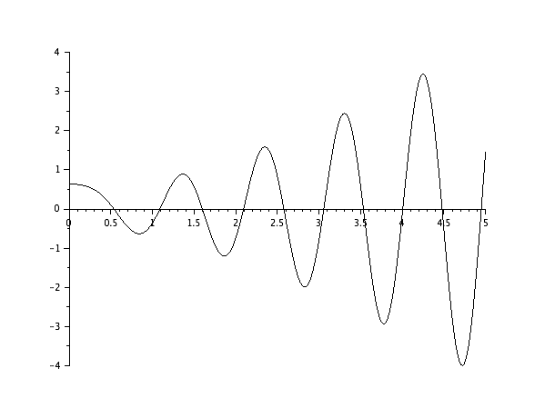
Figure 1: The plot shows the values of $T_{h_{\epsilon}}$ for $\mu_{\epsilon}:=\epsilon^{-2}\chi_{B_{\epsilon}}$ and $f=e^{-\pi|x|^{2}}$ and for $\epsilon\in(0,5)$, indicating if the triangular lattice is stable ($T_{h_{\epsilon}}>0$) or unstable.

2.3 Proof of Theorem 3

Let $f\in{\mathcal{F}}$ and let $\mu$ be written as $d\mu(x)=\rho(x)dx$ for some $\rho$ satisfying (1.5). With a similar argument as in the proof of Proposition 7, proving that ${\mathcal{E}}_{f,\mu}$ is minimized by $\Lambda$ in ${\mathcal{D}}$ is equivalent with proving the same for

$$E_{h}[L]:=\sum_{p\in L}{\vphantom{\sum}}^{\prime}\hat{f}(p)\hat{\rho}^{2}(p).$$ (2.47)

By Lemma 10 $\hat{f},\hat{\rho}\in{\mathcal{F}}$. Hence, $\Phi,G$ defined by $\Phi(|p|^{2}):=\hat{f}(p)$ and $G(|p|^{2}):=\hat{\rho}(p)$ are completely monotone. Since the product of two completely monotone functions is again completely monotone, the function $H=\Phi G^{2}$ is completely monotone. It follows (see e.g. [6, Prop 3.1]) that the triangular lattice $\Lambda$ is the unique minimizer in ${\mathcal{D}}$, up to rotation, of

$$E_{h}[L]=\sum_{p\in L}{\vphantom{\sum}}^{\prime}H(|p|^{2})=\sum_{p\in L}{\vphantom{\sum}}^{\prime}\hat{f}(p)\hat{\rho}(p)^{2}.$$ (2.48)

Acknowledgement.

LB is grateful for the support of the Mathematics Center Heidelberg (MATCH) during his stay in Heidelberg. He also acknowledges support from ERC advanced grant Mathematics of the Structure of Matter (project No. 321029) and from VILLUM FONDEN via the QMATH Centre of Excellence (grant No. 10059). HK is grateful about support from DFG grant 392124319. The authors also thank the referees for their interesting suggestions and comments.

References

• [1] M. Abramowitz and I. A. Stegun. Handbook of mathematical functions with formulas, graphs, and mathematical tables. U.S. Government Printing Office, Washington D.C., 1964.
• [2] A. Aftalion, X. Blanc, and F. Nier. Lowest Landau level functional and Bargmann spaces for Bose–Einstein condensates. J. Funct. Anal., 241:661–702, 2006.
• [3] D. Balagué, J. A. Carrillo, T. Laurent, and G. Raoul. Nonlocal interactions by repulsive-attractive potentials: radial ins/stability. Phys. D, 260:5–25, 2013.
• [4] A. J. Bernoff and C. M. Topaz. A primer of swarm equilibria. SIAM J. Appl. Dyn. Syst., 10(1):212–250, 2011.
• [5] L. Bétermin. Local variational study of 2d lattice energies and application to lennard-jones type interactions. Preprint. arXiv:1611.07820, 2016.
• [6] L. Bétermin. Two-dimensional Theta Functions and Crystallization among Bravais Lattices. SIAM J. Math. Anal., 48(5):3236–3269, 2016.
• [7] L. Bétermin. Local optimality of cubic lattices for interaction energies. Anal. Math. Phys., (online first) DOI:10.1007/s13324-017-0205-5, 2017.
• [8] L. Bétermin and H. Knüpfer. On Born’s conjecture about optimal distribution of charges for an infinite ionic crystal. Preprint. arXiv:1704.02887, 2017.
• [9] L. Bétermin and M. Petrache. Dimension reduction techniques for the minimization of theta functions on lattices. J. Math. Phys., 58:071902, 2017.
• [10] L. Bétermin and E. Sandier. Renormalized Energy and Asymptotic Expansion of Optimal Logarithmic Energy on the Sphere. Constr. Approx. , Special Issue: Approximation and Statistical Physics - Part I, 47(1):39–74, 2018.
• [11] L. Bétermin and P. Zhang. Minimization of energy per particle among Bravais lattices in $\mathbb{R}^{2}$: Lennard-Jones and Thomas-Fermi cases. Commun. Contemp. Math., 17(6):1450049, 2015.
• [12] X. Blanc. Geometry optimization for crystals in Thomas-Fermi type theories of solids. Comm. Partial Differential Equations, 26(3-4):651–696, 2001.
• [13] X. Blanc and M. Lewin. The Crystallization Conjecture: A Review. EMS Surv. in Math. Sci., 2:255–306, 2015.
• [14] J. A. Carrillo, S. Martin, and V. Panferov. A new interaction potential for swarming models. Phys. D, 260:112–126, 2013.
• [15] J.W.S. Cassels. On a Problem of Rankin about the Epstein Zeta-Function. Proceedings of the Glasgow Mathematical Association, 4:73–80, 7 1959.
• [16] X. Chen and Y. Oshita. An application of the modular function in nonlocal variational problems. Arch. Ration. Mech. Anal., 186(1):109–132, 2007.
• [17] R. Choksi, M. A. Peletier, and J. F. Williams. On the phase diagram for microphase separation of diblock copolymers: an approach via a nonlocal Cahn-Hilliard functional. SIAM J. Appl. Math., 69:1712–1738, 2008.
• [18] R. Choksi, M. A. Peletier, and J. F. Williams. On the phase diagram for microphase separation of diblock copolymers: an approach via a nonlocal Cahn-Hilliard functional. SIAM J. Appl. Math., 69(6):1712–1738, 2009.
• [19] H. Cohn and N. Elkies. New upper bounds on sphere packings I. Ann. of Math, 157:689–714, 2003.
• [20] H. Cohn and A. Kumar. Universally optimal distribution of points on spheres. J. Amer. Math. Soc., 20(1):99–148, 2007.
• [21] H. Cohn, A. Kumar, S. D. Miller, D. Radchenko, and M. Viazovska. The sphere packing problem in dimension 24. Ann. of Math, 185(3):1017–1033, 2017.
• [22] W.C. Connett and A.L. Schwartz. Fourier Analysis Off Groups. Contemp. Math., 137:169–176, 1992.
• [23] R. Coulangeon and A. Schürmann. Energy Minimization, Periodic Sets and Spherical Designs. Int. Math. Res. Not. IMRN, pages 829–848, 2012.
• [24] P. H. Diananda. Notes on Two Lemmas concerning the Epstein Zeta-Function. Proceedings of the Glasgow Mathematical Association, 6:202–204, 7 1964.
• [25] V. Ennola. A Lemma about the Epstein Zeta-Function. Proceedings of The Glasgow Mathematical Association, 6:198–201, 1964.
• [26] L. Flatley and F. Theil. Face-Centred Cubic Crystallization of Atomistic Configurations. Arch. Ration. Mech. Anal., 219(1):363–416, 2015.
• [27] B. A. Grzybowski, H. A. Stone, and G. M. Whitesides. Dynamics of self assembly of magnetized disks rotating at the liquid–air interface. Proc. Natl. Acad. Sci. USA, 99(7):4147–4151, 2002.
• [28] D. P. Hardin, E. B. Saff, and B. Simanek. Periodic Discrete Energy for Long-Range Potentials. J. Math. Phys., 55(12):123509, 2014.
• [29] D. M. Heyes and A. C. Branka. Lattice summations for spread out particles: Applications to neutral and charged systems. J. Chem. Phys., 138(3):034504, 2013.
• [30] H. Knüpfer, C. B. Muratov, and M. Novaga. Low density phases in a uniformly charged liquid. Comm. Math. Phys., 345(1):141–183, 2016.
• [31] L. De Luca and G. Friesecke. Crystallization in two dimensions and a discrete gauss-bonnet theorem. J. Nonlinear Sci., 28(1):69–90, 2018.
• [32] E. Mainini, P. Piovano, and U. Stefanelli. Finite crystallization in the square lattice. Nonlinearity, 27:717–737, 2014.
• [33] E. Mainini and U. Stefanelli. Crystallization in carbon nanostructures. Comm. Math. Phys., 328:545–571, 2014.
• [34] K. S. Miller and S. G. Samko. Completely monotonic functions. Integr. Transf. Spec. Funct., 12:389–402, 2001.
• [35] H. L. Montgomery. Minimal Theta Functions. Glasg. Math. J., 30(1):75–85, 1988.
• [36] F. Nier. A propos des fonctions Thêta et des réseaux d’Abrikosov. In Séminaire EDP-Ecole Polytechnique, 2006-2007.
• [37] S. Nonnenmacher and A. Voros. Chaotic Eigenfunctions in Phase Space. J. Stat. Phys., 92:431–518, 1998.
• [38] T. Ohta and K. Kawasaki. Equilibrium morphology of block copolymer melts. Macromolecules, 19(10):2621–2632, 1986.
• [39] R. A. Rankin. A Minimum Problem for the Epstein Zeta-Function. Proceedings of The Glasgow Mathematical Association, 1:149–158, 1953.
• [40] E. Sandier and S. Serfaty. From the Ginzburg-Landau Model to Vortex Lattice Problems. Comm. Math. Phys., 313(3):635–743, 2012.
• [41] P. Sarnak and A. Strömbergsson. Minima of Epstein’s Zeta Function and Heights of Flat Tori. Invent. Math., 165:115–151, 2006.
• [42] E. Stein and G. Weiss. Introduction to Fourier analysis on Euclidean spaces. Princeton University Press, Princeton, N.J., 1971. Princeton Mathematical Series, No. 32.
• [43] A. Süto. Crystalline Ground States for Classical Particles. Phys. Rev. Lett., 95, 2005.
• [44] A. Süto. Ground State at High Density. Comm. Math. Phys., 305:657–710, 2011.
• [45] F. Theil. A Proof of Crystallization in Two Dimensions. Comm. Math. Phys., 262(1):209–236, 2006.
• [46] C. M. Topaz and A. L. Bertozzi. Swarming patterns in a two-dimensional kinematic model for biological groups. SIAM J. Appl. Math., 65(1):152–174, 2004.
• [47] M. Viazovska. The sphere packing problem in dimension 8. Ann. of Math, 185(3):991–1015, 2017.