The Tamed Unadjusted Langevin Algorithm

Abstract

In this article, we consider the problem of sampling from a probability measure $\pi$ having a density on $\mathbb{R}^{d}$ proportional to $x\mapsto\mathrm{e}^{-U(x)}$. The Euler discretization of the Langevin stochastic differential equation (SDE) is known to be unstable, when the potential $U$ is superlinear. Based on previous works on the taming of superlinear drift coefficients for SDEs, we introduce the Tamed Unadjusted Langevin Algorithm (TULA) and obtain non-asymptotic bounds in $V$-total variation norm and Wasserstein distance of order $2$ between the iterates of TULA and $\pi$, as well as weak error bounds. Numerical experiments are presented which support our findings.

1 Introduction

The Unadjusted Langevin Algorithm (ULA) first introduced in the physics literature by [Par81] and popularized in the computational statistics community by [Gre83] and [GM94] is a technique to sample complex and high-dimensional probability distributions. This issue has far-reaching consequences in Bayesian statistics and machine learning [And+03], [Cot+13], aggregation of estimators [DT12] and molecular dynamics [LS16]. More precisely, let $\pi$ be a probability distribution on $\mathbb{R}^{d}$ which has density (also denoted by $\pi$) with respect to the Lebesgue measure given for all $x\in\mathbb{R}^{d}$ by,

$$\pi(x)=\mathrm{e}^{-U(x)}\big{/}\int_{\mathbb{R}^{d}}\mathrm{e}^{-U(y)}\mathrm{d}y\;,\quad\text{with}\quad\int_{\mathbb{R}^{d}}\mathrm{e}^{-U(y)}\mathrm{d}y<+\infty\;.$$

Assuming that $U:\mathbb{R}^{d}\to\mathbb{R}$ is continuously differentiable, the overdamped Langevin stochastic differential equation (SDE) associated with $\pi$ is given by

$$\mathrm{d}Y_{t}=-\nabla U(Y_{t})\mathrm{d}t+\sqrt{2}\mathrm{d}B_{t}\;,$$ (1)

where $(B_{t})_{t\geq 0}$ is a $d$-dimensional Brownian motion. The discrete time Markov chain associated with the ULA algorithm is obtained by the Euler-Maruyama discretization scheme of the Langevin SDE defined for $k\in\mathbb{N}$ by,

$$X_{k+1}=X_{k}-\gamma\nabla U(X_{k})+\sqrt{2\gamma}Z_{k+1}\;,\;X_{0}=x_{0}\;,$$ (2)

where $x_{0}\in\mathbb{R}^{d}$, $\gamma>0$ and $(Z_{k})_{k\in\mathbb{N}}$ are i.i.d. standard $d$-dimensional Gaussian variables. Under adequate assumptions on a globally Lipschitz $\nabla U$, non-asymptotic bounds in total variation and Wasserstein distances between the distribution of $(X_{k})_{k\in\mathbb{N}}$ and $\pi$ can be found in [Dal17], [DM17], [DM16]. However, the ULA algorithm is unstable if $\nabla U$ is superlinear i.e. $\liminf_{\left\|x\right\|\to+\infty}\left\|\nabla U(x)\right\|/\left\|x\right\|=+\infty$, see [RT96, Theorem 3.2], [MSH02] and [HJK11]. This is illustrated with a particular example in [MSH02, Lemma 6.3] where, the SDE (1) is considered in one dimension with $U(x)=x^{4}/4$ along with the associated Euler discretization (2) and it is shown that for all $\gamma>0$, if $\mathbb{E}\left[X_{0}^{2}\right]\geq 2/\gamma$, one obtains $\lim_{n\to+\infty}\mathbb{E}\left[X_{n}^{2}\right]=+\infty$. Moreover, the sample path $(X_{n})_{n\in\mathbb{N}}$ diverges to infinity with positive probability.

Until recently, either implicit numerical schemes, e.g. see [MSH02] and [HMS02], or adaptive stepsize schemes, e.g. see [LMS07], were used to address this problem. However, in the last few years, a new generation of explicit numerical schemes, which are computationally efficient, has been introduced by “taming” appropriately the superlinearly growing drift, see [HJK12] and [Sab13] for more details.

Nonetheless, with the exception of [MSH02], these works focus on the discretization of SDEs with superlinear coefficients in finite time. We aim at extending these techniques to sample from $\pi$, the invariant measure of (1). To deal with the superlinear nature of $\nabla U$, we introduce a family of drift functions $(G_{\gamma})_{\gamma>0}$ with $G_{\gamma}:\mathbb{R}^{d}\to\mathbb{R}^{d}$ indexed by the step size $\gamma$ which are close approximations of $\nabla U$ in a sense made precise below. Consider then the following Markov chain $(X_{k})_{k\in\mathbb{N}}$ defined for all $k\in\mathbb{N}$ by

$$X_{k+1}=X_{k}-\gamma G_{\gamma}(X_{k})+\sqrt{2\gamma}Z_{k+1}\;,\;X_{0}=x_{0}\;.$$ (3)

We suggest two different explicit choices for the family $(G_{\gamma})_{\gamma>0}$ based on previous studies on the tamed Euler scheme [HJK12], [Sab13], [HJ15]. Define for all $\gamma>0$, $H_{\gamma},H_{\gamma,c}:\mathbb{R}^{d}\to\mathbb{R}^{d}$ for all $x\in\mathbb{R}^{d}$ by

$$H_{\gamma}(x)=\frac{\nabla U(x)}{1+\gamma\left\|\nabla U(x)\right\|}\quad\text{and}\quad H_{\gamma,c}(x)=\left(\frac{\partial_{i}U(x)}{1+\gamma\left|\partial_{i}U(x)\right|}\right)_{i\in\left\{1,\ldots,d\right\}}\;,$$ (4)

where $\partial_{i}U$ is the $i^{\text{th}}$-coordinate of $\nabla U$. The Euler scheme (3) with $G_{\gamma}=H_{\gamma}$, respectively $G_{\gamma}=H_{\gamma,c}$, is referred to as the Tamed Unadjusted Langevin Algorithm (TULA), respectively the coordinate-wise Tamed Unadjusted Langevin Algorithm (TULAc).

Another line of work has focused on the Metropolis Adjusted Langevin Algorithm (MALA) that consists in adding a Metropolis-Hastings step to the ULA algorithm. [BH13] provides a detailed analysis of MALA in the case where the drift coefficient is superlinear. Note also that a normalization of the gradient was suggested in [RT96, Section 1.4.3] calling it MALTA (Metropolis Adjusted Langevin Truncated Algorithm) and analyzed in [Atc06] and [BV10].

The article is organized as follows. In Section 2, the Markov chain $(X_{k})_{k\in\mathbb{N}}$ defined by (3) is shown to be $V$-geometrically ergodic w.r.t. an invariant measure $\pi_{\gamma}$. Non-asymptotic bounds between the distribution of $(X_{k})_{k\in\mathbb{N}}$ and $\pi$ in total variation and Wasserstein distances are provided, as well as weak error bounds. In Section 3, the methodology is illustrated through numerical examples. Finally, proofs of the main results appear in Section 4.

Notations

Let $\mathcal{B}(\mathbb{R}^{d})$ denote the Borel $\sigma$-field of $\mathbb{R}^{d}$. Moreover, let $\operatorname{L}^{1}(\mu)$ be the set of $\mu$-integrable functions for $\mu$ a probability measure on $(\mathbb{R}^{d},\mathcal{B}(\mathbb{R}^{d}))$. Further, $\mu(f)=\int_{\mathbb{R}^{d}}f(x)\mathrm{d}\mu(x)$ for an $f\in\operatorname{L}^{1}(\mu)$. Given a Markov kernel $R$ on $\mathbb{R}^{d}$, for all $x\in\mathbb{R}^{d}$ and $f$ integrable under $R(x,\cdot)$, denote by $Rf(x)=\int_{\mathbb{R}^{d}}f(y)R(x,\mathrm{d}y)$. Let $V:\mathbb{R}^{d}\to\left[1,\infty\right)$ be a measurable function. The $V$-total variation distance between $\mu$ and $\nu$ is defined as $\|\mu-\nu\|_{V}=\sup_{\left|f\right|\leq V}\left|\mu(f)-\nu(f)\right|$. If $V=1$, then $\|\cdot\|_{V}$ is the total variation denoted by $\|\cdot\|_{\mathrm{TV}}$. Let $\mu$ and $\nu$ be two probability measures on a state space $\Omega$ with a given $\sigma$-algebra. If $\mu\ll\nu$, we denote by $\mathrm{d}\mu/\mathrm{d}\nu$ the Radon-Nikodym derivative of $\mu$ w.r.t. $\nu$. In that case, the Kullback-Leibler divergence of $\mu$ w.r.t. to $\nu$ is defined as

$$\operatorname{KL}(\mu|\nu)=\int_{\Omega}\frac{\mathrm{d}\mu}{\mathrm{d}\nu}\log\left(\frac{\mathrm{d}\mu}{\mathrm{d}\nu}\right)\mathrm{d}\nu\;.$$

We say that $\zeta$ is a transference plan of $\mu$ and $\nu$ if it is a probability measure on $(\mathbb{R}^{d}\times\mathbb{R}^{d},\mathcal{B}(\mathbb{R}^{d}\times\mathbb{R}^{d}))$ such that for any Borel set $\mathrm{A}$ of $\mathbb{R}^{d}$, $\zeta(\mathrm{A}\times\mathbb{R}^{d})=\mu(\mathrm{A})$ and $\zeta(\mathbb{R}^{d}\times\mathrm{A})=\nu(\mathrm{A})$. We denote by $\Pi(\mu,\nu)$ the set of transference plans of $\mu$ and $\nu$. Furthermore, we say that a couple of $\mathbb{R}^{d}$-random variables $(X,Y)$ is a coupling of $\mu$ and $\nu$ if there exists $\zeta\in\Pi(\mu,\nu)$ such that $(X,Y)$ are distributed according to $\zeta$. For two probability measures $\mu$ and $\nu$, we define the Wasserstein distance of order $p\geq 1$ as

$$W_{p}(\mu,\nu)=\left(\inf_{\zeta\in\Pi(\mu,\nu)}\int_{\mathbb{R}^{d}\times\mathbb{R}^{d}}\left\|x-y\right\|^{p}\mathrm{d}\zeta(x,y)\right)^{1/p}\;.$$

By [Vil09, Theorem 4.1], for all $\mu,\nu$ probability measure on $\mathbb{R}^{d}$, there exists a transference plan $\zeta^{\star}\in\Pi(\mu,\nu)$ such that for any coupling $(X,Y)$ distributed according to $\zeta^{\star}$, $W_{p}(\mu,\nu)=\mathbb{E}[\left\|X-Y\right\|^{p}]^{1/p}$.

For $u,v\in\mathbb{R}^{d}$, define the scalar product $\left\langle u,v\right\rangle=\sum_{i=1}^{d}u_{i}v_{i}$ and the Euclidian norm $\left\|u\right\|=\left\langle u,u\right\rangle^{1/2}$. Denote by $\mathbb{S}^{d-1}=\left\{u\in\mathbb{R}^{d}:\left\|u\right\|=1\right\}$. For $k\in\mathbb{N}$, $m,m^{\prime}\in\mathbb{N}^{*}$ and $\Omega,\Omega^{\prime}$ two open sets of $\mathbb{R}^{m},\mathbb{R}^{m^{\prime}}$ respectively, denote by $\mathrm{C}^{k}(\Omega,\Omega^{\prime})$, the set of $k$-times continuously differentiable functions. For $f\in\mathrm{C}^{2}(\mathbb{R}^{d},\mathbb{R})$, denote by $\nabla f$ the gradient of $f$, $\partial_{i}f$ the $i^{\text{th}}$-coordinate of $\nabla f$, $\Delta f$ the Laplacian of $f$ and $\nabla^{2}f$ the Hessian of $f$. Define then for $x\in\mathbb{R}^{d}$, $\left\|\nabla^{2}f(x)\right\|=\sup_{u\in\mathbb{S}^{d-1}}\left\|\nabla^{2}f(x)u\right\|$. For $k\in\mathbb{N}$ and $f\in\mathrm{C}^{k}(\mathbb{R}^{d},\mathbb{R})$, denote by $\operatorname{D}^{i}f$ the $i$-th derivative of $f$ for $i\in\left\{0,\ldots,k\right\}$, i.e. $\operatorname{D}^{i}f$ is a symmetric $i$-linear map defined for all $x\in\mathbb{R}^{d}$ and $j_{1},\ldots,j_{i}\in\left\{1,\ldots,d\right\}$ by $\operatorname{D}^{i}f(x)[e_{j_{1}},\ldots,e_{j_{i}}]=\partial_{j_{1}\ldots j_{i}}f(x)$ where $e_{1},\ldots,e_{d}$ is the canonical basis of $\mathbb{R}^{d}$. For $x\in\mathbb{R}^{d}$ and $i\in\left\{1,\ldots,k\right\}$, define $\left\|\operatorname{D}^{0}f(x)\right\|=\left|f(x)\right|$, $\left\|\operatorname{D}^{i}f(x)\right\|=\sup_{u_{1},\ldots,u_{i}\in\mathbb{S}^{d-1}}\operatorname{D}^{i}f(x)[u_{1},\ldots,u_{i}]$. Note that $\left\|\operatorname{D}^{1}f(x)\right\|=\left\|\nabla f(x)\right\|$ and $\left\|\operatorname{D}^{2}f(x)\right\|=\left\|\nabla^{2}f(x)\right\|$. For $m,m^{\prime}\in\mathbb{N}^{*}$, define

$$\mathrm{C}_{\mathrm{poly}}(\mathbb{R}^{m},\mathbb{R}^{m^{\prime}})=\Big{\{}f\in\mathrm{C}(\mathbb{R}^{m},\mathbb{R}^{m^{\prime}})|\exists C_{q},q\geq 0,\forall x\in\mathbb{R}^{m},\\ \left\|f(x)\right\|\leq C_{q}(1+\left\|x\right\|^{q})\Big{\}}\;.$$

For all $x\in\mathbb{R}^{d}$ and $M>0$, we denote by $\operatorname{B}(x,M)$ (respectively $\overline{\operatorname{B}}(x,M)$), the open (respectively close) ball centered at $x$ of radius $M$. In the sequel, we take the convention that for $n,p\in\mathbb{N}$, $n<p$ then $\sum_{p}^{n}=0$ and $\prod_{p}^{n}=1$.

2 Ergodicity and convergence analysis

distance	order of the upper bound	assumptions
$\left\|\delta_{x}R_{\gamma}^{n}-\pi\right\|_{V^{1/2}}$	$n\gamma\lambda^{n\gamma}V(x)+\sqrt{\gamma}$	A 1, A 2, H 1 and H 2
$W_{2}^{2}(\delta_{x}R_{\gamma}^{n},\pi)$	$n\gamma\lambda^{n\gamma}V(x)+\gamma$	A 1, A 2, H 1, H 2 and H 3
$W_{2}^{2}(\delta_{x}R_{\gamma}^{n},\pi)$	$n\gamma^{1+\beta}\lambda^{n\gamma}V(x)+\gamma^{1+\beta}$	A 1, A 2, H 2, H 3 and H 4

Table 1: Summary of the upper bounds on the distances between the distribution of the $n^{\text{th}}$ iteration of the Markov chain defined by (3) and $\pi$.

In this Section, under appropriate assumptions on $\nabla U$ and $G_{\gamma}$, we show that the diffusion process $(Y_{t})_{t\geq 0}$ defined by (1) and its discretization $(X_{k})_{k\in\mathbb{N}}$ defined by (3) satisfy a Foster-Lyapunov drift condition and are $V$-geometrically ergodic, see Section 2 and Section 2. Second, for all $k\in\mathbb{N}^{*}$, non-asymptotic bounds in $V$-norm between the distribution of $X_{k}$ and $\pi$ are established. Our next results give non-asymptotic bounds in Wasserstein distance of order $2$, under the additional assumption that $U$ is strongly convex. A summary of our main contributions is given in Table 1, where $\lambda\in\left[0,1\right)$. We conclude this part by non-asymptotic bounds on the bias and the variance of the ergodic average $n^{-1}\sum_{k=0}^{n-1}f(X_{k})$, $n\in\mathbb{N}^{*}$, used as an estimator of $\pi(f)$, for $f:\mathbb{R}^{d}\to\mathbb{R}$ sufficiently smooth.

Henceforth, it is assumed that $U$ is continuously differentiable. Consider the following assumptions on $U$.

H 1.

There exist $\ell,L\in\mathbb{R}_{+}$ such that for all $x,y\in\mathbb{R}^{d}$,

$$\left\|\nabla U(x)-\nabla U(y)\right\|\leq L\left\{1+\left\|x\right\|^{\ell}+\left\|y\right\|^{\ell}\right\}\left\|x-y\right\|\;.$$

H 2.

1. $\liminf_{\left\|x\right\|\to+\infty}\left\|\nabla U(x)\right\|=+\infty$.

2. $\liminf_{\left\|x\right\|\to+\infty}\left\langle\frac{x}{\left\|x\right\|},\frac{\nabla U(x)}{\left\|\nabla U(x)\right\|}\right\rangle>0$.

Note that under H 2, $\liminf_{\left\|x\right\|\to+\infty}U(x)=+\infty$, $U$ has a minimum $x^{\star}$ and $\nabla U(x^{\star})=0$. Without loss of generality, it is assumed that $x^{\star}=0$. It implies under H 1 that for all $x\in\mathbb{R}^{d}$,

$$\left\|\nabla U(x)\right\|\leq 2L\left\{1+\left\|x\right\|^{\ell+1}\right\}\;.$$ (5)

Besides, under H 2-ii), there exists $C\in\mathbb{R}$ such that for all $x\in\mathbb{R}^{d}$, $\left\langle-\nabla U(x),x\right\rangle\leq C$. By [MT93, Theorem 2.1], [IW89, Chapter IV, Theorems 2.3, 3.1] and [RT96, Theorem 2.1], (1) has a unique strong solution denoted $(Y_{t})_{t\geq 0}$. By [KS91, Section 5.4.C, Theorem 4.20], one constructs the associated strongly Markovian semigroup $(P_{t})_{t\geq 0}$ given for all $t\geq 0$, $x\in\mathbb{R}^{d}$ and $\mathsf{A}\in\mathcal{B}(\mathbb{R}^{d})$ by $P_{t}(x,\mathsf{A})=\mathbb{E}\left[\mathbbm{1}_{\mathsf{A}}(Y_{t})|Y_{0}=x\right]$. Consider the infinitesimal generator $\mathscr{A}$ associated with (1) defined for all $h\in\mathrm{C}^{2}(\mathbb{R}^{d})$ and $x\in\mathbb{R}^{d}$ by

$$\mathscr{A}h(x)=-\left\langle\nabla U(x),\nabla h(x)\right\rangle+\Delta h(x)\;,$$ (6)

and for any $a\in\mathbb{R}_{+}^{*}$, define the Lyapunov function $V_{a}:\mathbb{R}^{d}\to\left[1,+\infty\right)$ for all $x\in\mathbb{R}^{d}$ by

$$V_{a}(x)=\exp\left(a(1+\left\|x\right\|^{2})^{1/2}\right)\;.$$ (7)

Foster-Lyapunov conditions enable to control the moments of the diffusion process $(Y_{t})_{t\geq 0}$, see e.g. [MT93, Section 6] or [RT96, Theorem 2.2].

Proposition .

Assume H 1, H 2 and let $a\in\mathbb{R}^{*}_{+}$. There exists $b_{a}\in\mathbb{R}_{+}$ (given explicitly in the proof) such that for all $x\in\mathbb{R}^{d}$

$$\mathscr{A}V_{a}(x)\leq-aV_{a}(x)+ab_{a}\;$$ (8)

and

$$\sup_{t\geq 0}P_{t}V_{a}(x)\leq V_{a}(x)+b_{a}\;.$$

Moreover, there exist $C_{a}\in\mathbb{R}_{+}$ and $\rho_{a}\in\left[0,1\right)$ such that for all $t\in\mathbb{R}_{+}$ and probability measures $\mu_{0},\nu_{0}$ on $(\mathbb{R}^{d},\mathcal{B}(\mathbb{R}^{d}))$ satisfying $\mu_{0}(V_{a})+\nu_{0}(V_{a})<+\infty$,

$$\left\|\mu_{0}P_{t}-\nu_{0}P_{t}\right\|_{V_{a}}\leq C_{a}\rho_{a}^{t}\left\|\mu_{0}-\nu_{0}\right\|_{V_{a}}\;,\;\left\|\mu_{0}P_{t}-\pi\right\|_{V_{a}}\leq C_{a}\rho_{a}^{t}\mu_{0}(V_{a})\;.$$ (9)

Proof.

The proof is postponed to Section 4.1. ∎

The Markov chain $(X_{k})_{k\in\mathbb{N}}$ defined in (3) is a discrete-time approximation of the diffusion $(Y_{t})_{t\geq 0}$. To control the total variation and Wasserstein distances of the marginal distributions of $(X_{k})_{k\in\mathbb{N}}$ and $(Y_{t})_{t\geq 0}$, it is necessary to assume that for $\gamma>0$ small enough, $G_{\gamma}$ and $\nabla U$ are close. This is formalized by A 1. Under the additional assumption A 2, we obtain the stability and ergodicity of $(X_{k})_{k\in\mathbb{N}}$.

A 1.

For all $\gamma>0$, $G_{\gamma}$ is continuous. There exist $\alpha\geq 0$, $C_{\alpha}<+\infty$ such that for all $\gamma>0$ and $x\in\mathbb{R}^{d}$,

$$\left\|G_{\gamma}(x)-\nabla U(x)\right\|\leq\gamma C_{\alpha}\left(1+\left\|x\right\|^{\alpha}\right)\;.$$

Note that under H 1, A 1 and by (5), we have for all $x\in\mathbb{R}^{d}$

$$\left\|G_{\gamma}(x)\right\|\leq 2L\left\{1+\left\|x\right\|^{\ell+1}\right\}+\gamma C_{\alpha}\left(1+\left\|x\right\|^{\alpha}\right)\;.$$ (10)

A 2.

For all $\gamma>0$, $\liminf_{\left\|x\right\|\to+\infty}\left\langle\frac{x}{\left\|x\right\|},G_{\gamma}(x)\right\rangle-\frac{\gamma}{2\left\|x\right\|}\left\|G_{\gamma}(x)\right\|^{2}>0$.

Lemma .

Assume H 1 and H 2. Let $\gamma>0$ and $G_{\gamma}$ be equal to $H_{\gamma}$ or $H_{\gamma,c}$ defined in (4). Then A 1 and A 2 are satisfied.

Proof.

The proof is postponed to Section 4.2. ∎

The Markov kernel $R_{\gamma}$ associated with (3) is given for all $\gamma>0$ , $x\in\mathbb{R}^{d}$ and $\mathsf{A}\in\mathcal{B}(\mathbb{R}^{d})$ by

$$R_{\gamma}(x,\mathsf{A})=(2\uppi)^{-d/2}\int_{\mathbb{R}^{d}}\mathbbm{1}_{\mathsf{A}}\left(x-\gamma G_{\gamma}(x)+\sqrt{2\gamma}z\right)\mathrm{e}^{-\left\|z\right\|^{2}/2}\mathrm{d}z\;.$$ (11)

We then obtain the counterpart of Section 2 for the Markov chain $(X_{k})_{k\in\mathbb{N}}$.

Proposition .

Assume H 1, A 1, A 2 and let $\gamma\in\mathbb{R}_{+}^{*}$. There exist $M,\ae,b\in\mathbb{R}^{*}_{+}$ (given explicitly in the proof) satisfying for all $x\in\mathbb{R}^{d}$

$$R_{\gamma}V_{\ae}(x)\leq\mathrm{e}^{-\ae^{2}\gamma}V_{\ae}(x)+\gamma b\mathbbm{1}_{\overline{\operatorname{B}}(0,M)}(x)\;.$$ (12)

In addition, $R_{\gamma}$ has a unique invariant measure $\pi_{\gamma}$, $R_{\gamma}$ is $V_{\ae}$-geometrically ergodic w.r.t. $\pi_{\gamma}$.

Proof.

The proof is postponed to Section 4.3. ∎

Note that a straightforward induction of (12) gives for all $n\in\mathbb{N}$ and $x\in\mathbb{R}^{d}$,

$$R_{\gamma}^{n}V_{\ae}(x)\leq\mathrm{e}^{-n\ae^{2}\gamma}V_{\ae}(x)+\{(b\gamma)(1-\mathrm{e}^{-n\ae^{2}\gamma})\}/(1-\mathrm{e}^{-\ae^{2}\gamma})\;.$$

Using $1-\mathrm{e}^{-\ae^{2}\gamma}=\int_{0}^{\gamma}\ae^{2}\mathrm{e}^{-\ae^{2}t}\mathrm{d}t\geq\gamma\ae^{2}\mathrm{e}^{-\ae^{2}\gamma}$, we get for all $n\in\mathbb{N}$

$$R_{\gamma}^{n}V_{\ae}(x)\leq\mathrm{e}^{-\ae^{2}n\gamma}V_{\ae}(x)+(b/\ae^{2})\mathrm{e}^{\ae^{2}\gamma}\;.$$ (13)

In the following result, we compare the discrete and continuous time processes $(X_{k})_{k\in\mathbb{N}}$ and $(Y_{t})_{t\geq 0}$ using Girsanov’s theorem and Pinsker’s inequality, see [Dal17] and [DM17, Theorem 10] for similar arguments.

Theorem 1.

Assume H 1, H 2, A 1 and A 2. Let $\gamma_{0}>0$. There exist $C>0$ and $\lambda\in\left(0,1\right)$ such that for all $\gamma\in\left(0,\gamma_{0}\right]$, $x\in\mathbb{R}^{d}$ and $n\in\mathbb{N}$,

$$\left\|\delta_{x}R_{\gamma}^{n}-\pi\right\|_{V_{\ae}^{1/2}}\leq C\left(n\gamma\lambda^{n\gamma}V_{\ae}(x)+\sqrt{\gamma}\right)\;,$$ (14)

where $\ae$ is defined in Section 2 and for all $\gamma\in\left(0,\gamma_{0}\right]$,

$$\left\|\pi_{\gamma}-\pi\right\|_{V_{\ae}^{1/2}}\leq C\sqrt{\gamma}\;.$$ (15)

Proof.

The proof is postponed to Section 4.4. ∎

By adding strong convexity for the potential, one obtains the corresponding bounds for the Wasserstein distance of order $2$.

H 3.

$U$ is strongly convex, i.e. there exists $m>0$ such that for all $x,y\in\mathbb{R}^{d}$,

$$\left\langle\nabla U(x)-\nabla U(y),x-y\right\rangle\geq m\left\|x-y\right\|^{2}\;.$$

By coupling $(Y_{t})_{t\geq 0}$ and the linear interpolation of $(X_{k})_{k\in\mathbb{N}}$ with the same Brownian motion, the following result is obtained.

Theorem 2.

Assume A 1, A 2, H 1, H 2 and H 3. Let $\gamma_{0}>0$. There exist $C>0$ and $\lambda\in\left(0,1\right)$ such that for all $x\in\mathbb{R}^{d}$, $\gamma\in\left(0,\gamma_{0}\right]$ and $n\in\mathbb{N}$,

$$W_{2}^{2}(\delta_{x}R_{\gamma}^{n},\pi)\leq C\left(n\gamma\lambda^{n\gamma}V_{\ae}(x)+\gamma\right)\;,$$ (16)

where $\ae$ is defined in Section 2 and for all $\gamma\in\left(0,\gamma_{0}\right]$,

$$W_{2}^{2}(\pi_{\gamma},\pi)\leq C\gamma\;.$$ (17)

Proof.

The proof is postponed to Section 4.5. ∎

If $U\in\mathrm{C}^{2}(\mathbb{R}^{d},\mathbb{R})$ and under the following assumption on $\nabla^{2}U$, the bound can be improved.

H 4.

$U$ is twice continuously differentiable and there exist $\nu,L_{H}\in\mathbb{R}_{+}$ and $\beta\in\left[0,1\right]$ such that for all $x,y\in\mathbb{R}^{d}$,

$$\left\|\nabla^{2}U(x)-\nabla^{2}U(y)\right\|\leq L_{H}\left\{1+\left\|x\right\|^{\nu}+\left\|y\right\|^{\nu}\right\}\left\|x-y\right\|^{\beta}\;.$$

It is shown in Section 4.5 that H 4 implies H 1.

Theorem 3.

Assume A 1, A 2, H 2, H 3 and H 4. Let $\gamma_{0}>0$. There exist $C>0$ and $\lambda\in\left(0,1\right)$ such that for all $x\in\mathbb{R}^{d}$, $\gamma\in\left(0,\gamma_{0}\right]$ and $n\in\mathbb{N}$,

$$W_{2}^{2}(\delta_{x}R_{\gamma}^{n},\pi)\leq C\left(n\gamma^{1+\beta}\lambda^{n\gamma}V_{\ae}(x)+\gamma^{1+\beta}\right)\;,$$ (18)

where $\ae$ is defined in Section 2 and for all $\gamma\in\left(0,\gamma_{0}\right]$,

$$W_{2}^{2}(\pi_{\gamma},\pi)\leq C\gamma^{1+\beta}\;.$$ (19)

Proof.

The proof is postponed to Section 4.5. ∎

The exponent of $\gamma$ in (16) is improved from $1$ to $1+\beta$. In particular, if $\nabla^{2}U$ is Lipschitz, $\nu=0$, $\beta=1$, and [DM16, Theorem 8] is recovered.

Let $(X_{k})_{k\in\mathbb{N}}$ be the Markov chain defined in (3). To study the empirical average $(1/n)\sum_{k=0}^{n-1}\{f(X_{k})-\pi(f)\}$ for $n\in\mathbb{N}^{*}$, we follow a method introduced in [MST10] and based on the Poisson equation. For $f$ a $\pi$-integrable function, the Poisson equation associated with the generator $\mathscr{A}$ defined in (6) is given for all $x\in\mathbb{R}^{d}$ by

$$\mathscr{A}\phi(x)=-\left(f(x)-\pi(f)\right)\;,$$ (20)

where $\phi$, if it exists, is a solution of the Poisson equation. This equation has proved to be a useful tool to analyze additive functionals of diffusion processes, see e.g. [CCG12] and references therein. The existence and regularity of a solution of the Poisson equation has been investigated in [GM96], [PV01], [Kop15], [Gor+16]. In that purpose, the following additional assumption on $U$ is necessary.

H 5.

$U\in\mathrm{C}^{4}(\mathbb{R}^{d},\mathbb{R})$ and $\left\|\operatorname{D}^{i}U\right\|\in\mathrm{C}_{\mathrm{poly}}(\mathbb{R}^{d},\mathbb{R}_{+})$ for $i\in\left\{1,\ldots,4\right\}$.

Theorem 4.

Assume H 2, H 5, A 1 and A 2. Let $f\in\mathrm{C}^{3}(\mathbb{R}^{d},\mathbb{R})$ be such that $\left\|\operatorname{D}^{i}f\right\|\in\mathrm{C}_{\mathrm{poly}}(\mathbb{R}^{d},\mathbb{R}_{+})$ for $i\in\left\{0,\ldots,3\right\}$. Let $\gamma_{0}>0$ and $(X_{k})_{k\in\mathbb{N}}$ be the Markov chain defined by (3) and starting at $X_{0}=0$. There exists $C>0$ such that for all $\gamma\in\left(0,\gamma_{0}\right]$ and $n\in\mathbb{N}^{*}$,

$$\left|\mathbb{E}\left[\frac{1}{n}\sum_{k=0}^{n-1}f(X_{k})-\pi(f)\right]\right|\leq C\left(\gamma+\frac{1}{n\gamma}\right)$$ (21)

and

$$\mathbb{E}\left[\left(\frac{1}{n}\sum_{k=0}^{n-1}f(X_{k})-\pi(f)\right)^{2}\right]\leq C\left(\gamma^{2}+\frac{1}{n\gamma}\right)\;.$$ (22)

Proof.

The proof is postponed to Section 4.6. ∎

Note that the standard rates of convergence are recovered, see [MST10, Theorems 5.1, 5.2].

3 Numerical examples

We illustrate our theoretical results using three numerical examples.

Multivariate Gaussian variable in high dimension

We first consider a multivariate Gaussian variable in dimension $d\in\{100,1000\}$ of mean $0$ and covariance matrix $\Sigma=\operatorname{diag}(1,\ldots,d)$. The potential $U:\mathbb{R}^{d}\to\mathbb{R}$ defined for all $x\in\mathbb{R}^{d}$ by $U(x)=(1/2)x^{\operatorname{T}}\Sigma^{-1}x$ is $d^{-1}$-strongly convex and $1$-gradient Lipschitz. The assumptions H 1, H 2, H 3, H 4 with $\beta=1$ and H 5 are thus satisfied. Note that in this case, ULA is stable and the analysis of [Dal17], [DM17], [DM16] valid. Nevertheless, implementing TULA and TULAc on this example is still of interest. Indeed, some Bayesian posterior distributions have intricate expressions and identifying the superlinear part in the gradient $\nabla U$ may be a difficult task. Within this context, we check the robustness of TULA and TULAc with respect to (globally) Lipschitz $\nabla U$.

We also consider in Appendix F a badly conditioned multivariate Gaussian variable in dimension $d=100$ of mean $0$ and covariance matrix $\Sigma=\operatorname{diag}(10^{-5},1,\ldots,1)$. In this example, ULA requires a step size of order $10^{-5}$ to be stable which implies a large number of iterations to obtain relevant results. On the other side, TULA and TULAc are applicable with a step size of order $10^{-2}$ and within a relatively small number of iterations, valid results for the axes $2$ to $100$ are obtained.

Double well

The potential is defined for all $x\in\mathbb{R}^{d}$ by $U(x)=(1/4)\left\|x\right\|^{4}-(1/2)\left\|x\right\|^{2}$. We have $\nabla U(x)=(\left\|x\right\|^{2}-1)x$ and $\nabla^{2}U(x)=(\left\|x\right\|^{2}-1)\operatorname{Id}+2xx^{\operatorname{T}}$. We get $\left\|\nabla^{2}U(x)\right\|=3\left\|x\right\|^{2}-1$, $\left\langle x,\nabla U(x)\right\rangle=\left\|x\right\|\left\|\nabla U(x)\right\|$ for $\left\|x\right\|\geq 1$ and

$$\left\|\nabla^{2}U(x)-\nabla^{2}U(y)\right\|\leq 3\left(\left\|x\right\|+\left\|y\right\|\right)\left\|x-y\right\|\;,$$

so that H 1, H 2, H 4 with $\beta=1$ and H 5 are satisfied.

Ginzburg-Landau model

This model of phase transitions in physics [LFR17, Section 6.2] is defined on a three-dimensional $d=p^{3}$ lattice for $p\in\mathbb{N}^{*}$ and the potential is given for $x=\left(x_{ijk}\right)_{i,j,k\in\left\{1,\ldots,p\right\}}\in\mathbb{R}^{d}$ by

$$U(x)=\sum_{i,j,k=1}^{p}\left\{\frac{1-\tau}{2}x_{ijk}^{2}+\frac{\tau\alpha}{2}\left\|\tilde{\nabla}x_{ijk}\right\|^{2}+\frac{\tau\lambda}{4}x_{ijk}^{4}\right\}\;,$$

where $\alpha,\lambda,\tau>0$ and $\tilde{\nabla}x_{ijk}=(x_{i_{+}jk}-x_{ijk},x_{ij_{+}k}-x_{ijk},x_{ijk_{+}}-x_{ijk})$ with $i_{\pm}=i\pm 1\;\text{mod}\;p$ and similarly for $j_{\pm},k_{\pm}$. In the simulations, $p$ is equal to $10$. We have

$$\nabla U(x)=\Big{\{}\tau\alpha\left(6x_{ijk}-x_{i_{+}jk}-x_{ij_{+}k}-x_{ijk_{+}}-x_{i_{-}jk}-x_{ij_{-}k}-x_{ijk_{-}}\right)\\ +(1-\tau)x_{ijk}+\tau\lambda x_{ijk}^{3}\Big{\}}_{i,j,k\in\left\{1,\ldots,p\right\}}\;,$$

and

$$\nabla^{2}U(x)=\operatorname{diag}\left(\left(1-\tau+6\tau\alpha+3\tau\lambda x_{ijk}^{2}\right)_{i,j,k\in\left\{1,\ldots,p\right\}}\right)+M\;,$$

where $M\in\mathbb{R}^{d\times d}$ is a constant matrix. H 1, H 4 with $\beta=1$ and H 5 are thus satisfied. Using that $x\mapsto\sum_{i,j,k=1}^{p}\left\|\tilde{\nabla}x_{ijk}\right\|^{2}$ is convex by composition of convex functions and its gradient evaluated in $0$ is $0$, we have for all $x\in\mathbb{R}^{d}$,

$$\left\langle x,\nabla U(x)\right\rangle\geq\sum_{i,j,k=1}^{p}\{(1-\tau)x_{ijk}^{2}+\tau\lambda x_{ijk}^{4}\}\;.$$

By Cauchy-Schwarz inequality, $\left\{\sum_{i,j,k=1}^{p}x_{ijk}^{2}\right\}^{2}\leq d\sum_{i,j,k=1}^{p}x_{ijk}^{4}$, and for all $x\in\mathbb{R}^{d}$, $\left\|x\right\|^{2}\geq(2\left|1-\tau\right|d)/(\tau\lambda)$, we get $\left\langle x,\nabla U(x)\right\rangle\geq\{(\tau\lambda)/2\}\sum_{i,j,k=1}^{p}x_{ijk}^{4}$. Besides, we have

$$\left\|\nabla U(x)\right\|\leq(\left|1-\tau\right|+12\tau\alpha)\left\|x\right\|+\tau\lambda\left\|(x_{ijk}^{3})_{i,j,k\in\left\{1,\ldots,p\right\}}\right\|\;.$$

Let $a,b,c\in\left\{1,\ldots,p\right\}$ be such that $\left|x_{abc}\right|=\max\left|x_{ijk}\right|$. We get

$$\left\|x\right\|\left\|(x_{ijk}^{3})_{i,j,k\in\left\{1,\ldots,p\right\}}\right\|\leq dx_{abc}^{4}\leq d\sum_{i,j,k=1}^{p}x_{ijk}^{4}\;.$$

Finally, for $\left\|x\right\|^{2}\geq\max\{1,(2\left|1-\tau\right|d)/(\tau\lambda)\}$, we obtain

$$\left\|x\right\|\left\|\nabla U(x)\right\|\leq\left\{\frac{2d\left|1-\tau\right|}{\tau\lambda}+\frac{24\alpha d}{\lambda}+2d\right\}\left\langle x,\nabla U(x)\right\rangle\;,$$

and H 2 is satisfied.

We benchmark TULA and TULAc against ULA given by (2), MALA and a Random Walk Metropolis-Hastings with a Gaussian proposal (RWM). TMALA (Tamed Metropolis Adjusted Langevin Algorithm) and TMALAc (coordinate-wise Tamed Metropolis Adjusted Langevin Algorithm), the Metropolized versions of TULA and TULAc, are also included in the numerical tests. Their theoretical analysis is similar to the one of MALTA [Atc06, Proposition 2.1].

Since double well and Ginzburg-Landau models are coordinate-wise exchangeable, the results are provided only for their first coordinate. The Markov chains associated with these models are started at $X_{0}=0,(10,0^{\otimes(d-1)}),(100,0^{\otimes(d-1)})$, $(1000,0^{\otimes(d-1)})$ and for the multivariate Gaussian at a random vector of norm $0,10,100,1000$. For the Gaussian and double well examples, for each initial condition, algorithm, step size $\gamma\in\left\{10^{-3},10^{-2},10^{-1}\right\}$, we run $100$ independent Markov chains started at $X_{0}$ of $10^{6}$ samples (respectively $10^{5}$) in dimension $d=100$ (respectively $d=1000$). For the Ginzburg-Landau model, we run $100$ independent Markov chains started at $X_{0}$ of $10^{5}$ samples. For each run, we estimate the 1st and 2nd moment for the first and last coordinate, i.e. $\int_{\mathbb{R}^{d}}x_{i}\pi(x)\mathrm{d}x$ for $i\in\left\{1,d\right\}$, by the empirical average and we compute the boxplots of the errors. For ULA, if the norm of $X_{k}$ for $k\in\mathbb{N}$ exceeds $10^{5}$, the chain is stopped and for this step size $\gamma$ the trajectory of ULA is not taken into account. For MALA, RWM, TMALA and TMALAc, if the acceptance ratio is below $0.05$, we similarly do not take into account the corresponding trajectories.

For the three examples and for $i\in\left\{1,\ldots,d\right\}$, $\int_{\mathbb{R}^{d}}x_{i}\pi(x)\mathrm{d}x=0$. By symmetry, for the double well, we have for $i\in\left\{1,\ldots,d\right\}$ and $r\in\mathbb{R}_{+}$,

$$\mathbb{E}\left[X_{i}^{2}\right]=d^{-1}\int_{\mathbb{R}_{+}}r^{2}\nu(r)\mathrm{d}r\Big{/}\int_{\mathbb{R}_{+}}\nu(r)\mathrm{d}r\;,\quad\nu(r)=r^{d-1}\exp\left\{(r^{2}/2)-(r^{4}/4)\right\}\;.$$

A Random Walk Metropolis run of $10^{7}$ samples gives $\int_{\mathbb{R}^{d}}x_{i}^{2}\pi(x)\mathrm{d}x\approx 0.104\pm 0.001$ for $d=100$ and $\int_{\mathbb{R}^{d}}x_{i}^{2}\pi(x)\mathrm{d}x\approx 0.032\pm 0.001$ for $d=1000$.

Because of lack of space, we only display some boxplots in Figures 1, 2, 3 and 4. The Python code and all the figures are available at https://github.com/nbrosse/TULA. We remark that TULA, TULAc and to a lesser extent, TMALA and TMALAc, have a stable behavior even with large step sizes and starting far from the origin. This is particularly visible in Figures 2 and 4 where ULA diverges (i.e. $\liminf_{k\to+\infty}\mathbb{E}\left[\left\|X_{k}\right\|\right]=+\infty$) and MALA does not move even for small step sizes $\gamma=10^{-3}$. Note however the existence of a bias for ULA, TULA and TULAc in Figure 3. Finally, comparison of the results shows that TULAc is preferable to TULA.

Note that other choices are possible for $G_{\gamma}$, depending on the model under study. For example, in the case of the double well, we could ”tame” only the superlinear part of $\nabla U$, i.e. consider for all $\gamma>0$ and $x\in\mathbb{R}^{d}$,

$$G_{\gamma}(x)=\frac{\left\|x\right\|^{2}x}{1+\gamma\left\|x\right\|^{2}}-x\;.$$ (23)

A 1 is satisfied and we have

$$\left\langle\frac{x}{\left\|x\right\|},G_{\gamma}(x)\right\rangle-\frac{\gamma}{2\left\|x\right\|}\left\|G_{\gamma}(x)\right\|^{2}=\frac{\left\|x\right\|^{3}}{1+\gamma\left\|x\right\|^{2}}\Big{\{}1+\gamma-\frac{\gamma}{2}\frac{\left\|x\right\|^{2}}{1+\gamma\left\|x\right\|^{2}}\Big{\}}$$

$$\phantom{------------------------}-\left\|x\right\|\left\{1+(\gamma/2)\right\}\;,$$

$$\liminf_{\left\|x\right\|\to+\infty}\left\langle\frac{x}{\left\|x\right\|^{2}},G_{\gamma}(x)\right\rangle-\frac{\gamma}{2\left\|x\right\|^{2}}\left\|G_{\gamma}(x)\right\|^{2}=\frac{\gamma^{-1}-\gamma}{2}\;.$$

A 2 is satisfied if and only if $\gamma\in\left(0,1\right)$. It is striking to see that this theoretical threshold is clearly visible on the simulations. The algorithm (3) with $G_{\gamma}$ defined by (23) obtains similar results as TULAc for $\gamma<1$ but for $\gamma=1$, the algorithm diverges.

Given the results of the numerical experiments, TULAc should be chosen over ULA to sample from general probability distributions. Indeed, TULAc has similar results as ULA when the step size is small and is more stable when using larger step sizes.

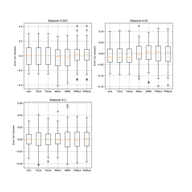
Figure 1: Boxplots of the error on the first moment for the multivariate Gaussian (first coordinate) in dimension $1000$ starting at $0$ for different step sizes.

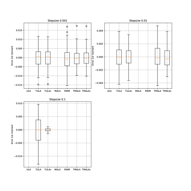
Figure 2: Boxplots of the error on the first moment for the double well in dimension $100$ starting at $(100,0^{\otimes 99})$ for different step sizes.

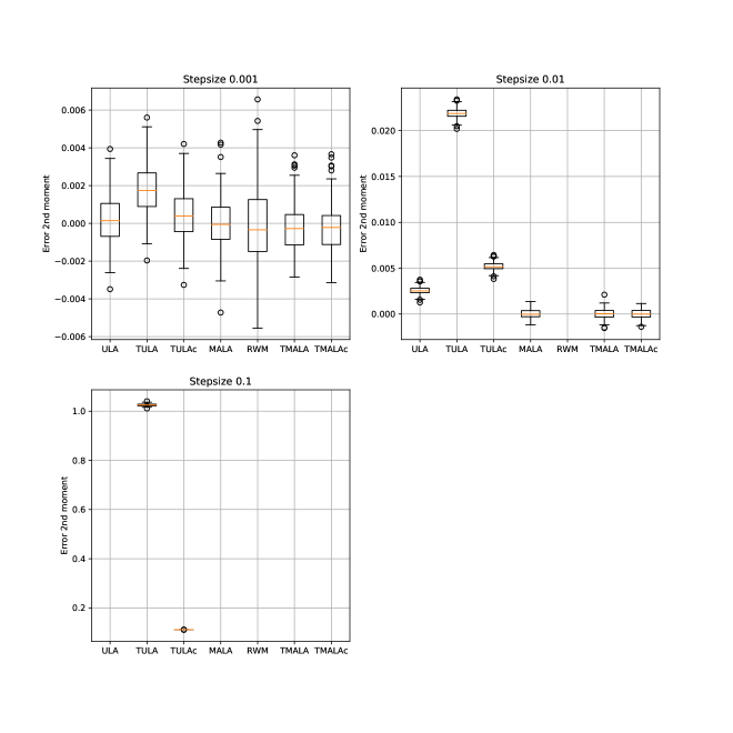
Figure 3: Boxplots of the error on the second moment for the double well in dimension $100$ starting at $0$ for different step sizes.

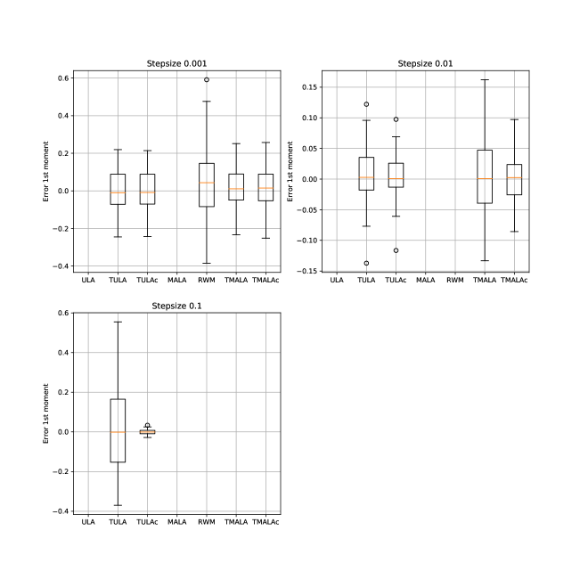
Figure 4: Boxplots of the error on the first moment for the Ginzburg-Landau model in dimension $1000$ starting at $(100,0^{\otimes 999})$ for different step sizes.

4 Proofs

4.1 Proof of Section 2

We have for all $x\in\mathbb{R}^{d}$,

$$\frac{\mathscr{A}V_{a}(x)}{aV_{a}(x)}=-\left\langle\nabla U(x),\frac{x}{(1+\left\|x\right\|^{2})^{1/2}}\right\rangle+\frac{a\left\|x\right\|^{2}}{1+\left\|x\right\|^{2}}+\frac{d}{(1+\left\|x\right\|^{2})^{1/2}}\\ -\frac{\left\|x\right\|^{2}}{(1+\left\|x\right\|^{2})^{3/2}}\;.$$ (24)

By H 2-ii) and using $s\mapsto s/(1+s^{2})^{1/2}$ is non-decreasing for $s\geq 0$, there exist $M_{1},\kappa\in\mathbb{R}^{*}_{+}$ such that for all $x\in\mathbb{R}^{d}$, $\left\|x\right\|\geq M_{1}$, $\left\langle\nabla U(x),x(1+\left\|x\right\|^{2})^{-1/2}\right\rangle\geq\kappa\left\|\nabla U(x)\right\|$. By H 2-i), there exists $M_{2}\geq M_{1}$ such that for all $x\in\mathbb{R}^{d}$, $\left\|x\right\|\geq M_{2}$, $\left\|\nabla U(x)\right\|\geq\kappa^{-1}\{1+a+d(1+M_{1}^{2})^{-1/2}\}$. We then have for all $x\in\mathbb{R}^{d}$, $\left\|x\right\|\geq M_{2}$, $\mathscr{A}V_{a}(x)\leq-aV_{a}(x)$. Define

$$b_{a}=\exp(a(1+M_{2}^{2})^{1/2})\{2L(1+M_{2}^{\ell+1})+a+d\}\;.$$

Combining (5) and (24) gives (8). By [MT93, Theorem 1.1], we get $P_{t}V_{a}(x)\leq\mathrm{e}^{-at}V_{a}(x)+b_{a}(1-\mathrm{e}^{-at})$. The second statement is a consequence of [RT96, Theorem 2.2] and [MT93, Theorem 6.1].

4.2 Proof of Section 2

Let $\gamma>0$. We have for all $x\in\mathbb{R}^{d}$, $\left\|H_{\gamma}(x)-\nabla U(x)\right\|\leq\gamma\left\|\nabla U(x)\right\|^{2}$ and

$$\left\|H_{\gamma,c}(x)-\nabla U(x)\right\|\leq\gamma\left\{\sum_{i=1}^{d}\left(\partial_{i}U(x)\right)^{4}\right\}^{1/2}\leq\gamma\left\|\nabla U(x)\right\|^{2}\;.$$

By (5), A 1 is satisfied. Define for all $x\in\mathbb{R}^{d}$, $x\neq 0$,

$$A_{\gamma}(x)=\left\langle\frac{x}{\left\|x\right\|},H_{\gamma}(x)\right\rangle-\frac{\gamma}{2\left\|x\right\|}\left\|H_{\gamma}(x)\right\|^{2}\;.$$

By H 2-ii), there exist $M_{1},\kappa>0$ such that for all $x\in\mathbb{R}^{d}$, $\left\|x\right\|\geq M_{1}$, $\left\langle x,\nabla U(x)\right\rangle\geq\kappa\left\|x\right\|\left\|\nabla U(x)\right\|$. We get then for all $x\in\mathbb{R}^{d}$, $\left\|x\right\|\geq M_{1}$,

$$A_{\gamma}(x) =\frac{1}{2\left\|x\right\|\{1+\gamma\left\|\nabla U(x)\right\|\}}\left\{2\left\langle x,\nabla U(x)\right\rangle-\left\|\nabla U(x)\right\|\frac{\gamma\left\|\nabla U(x)\right\|}{1+\gamma\left\|\nabla U(x)\right\|}\right\}$$

$$\geq\frac{\left\|\nabla U(x)\right\|}{1+\gamma\left\|\nabla U(x)\right\|}\frac{2\kappa\left\|x\right\|-1}{2\left\|x\right\|}\;.$$

By H 2-i), there exist $M_{2},C>0$ such that for all $x\in\mathbb{R}^{d}$, $\left\|x\right\|\geq M_{2}$, $\left\|\nabla U(x)\right\|\geq C$. Using that $s\mapsto s(1+\gamma s)^{-1}$ is non-decreasing for $s\geq 0$, we get for all $x\in\mathbb{R}^{d}$, $\left\|x\right\|\geq\max(\kappa^{-1},M_{1},M_{2})$, $A_{\gamma}(x)\geq(\kappa C)/\{2(1+\gamma C)\}$.

Define for all $x\in\mathbb{R}^{d}$, $x\neq 0$,

$$B_{\gamma}(x)=\left\langle\frac{x}{\left\|x\right\|},H_{\gamma,c}(x)\right\rangle-\frac{\gamma}{2\left\|x\right\|}\left\|H_{\gamma,c}(x)\right\|^{2}\;.$$

We have for all $x\in\mathbb{R}^{d}$, $\gamma\left\|H_{\gamma,c}(x)\right\|\leq\sqrt{d}$ and for all $x\in\mathbb{R}^{d}$, $\left\|x\right\|\geq M_{1}$,

$$\left\langle x,\left(\frac{\partial_{i}U(x)}{1+\gamma\left|\partial_{i}U(x)\right|}\right)_{i\in\left\{1,\ldots,d\right\}}\right\rangle\geq\frac{\kappa\left\|x\right\|\left\|\nabla U(x)\right\|}{1+\gamma\max_{i\in\left\{1,\ldots,d\right\}}\left|\partial_{i}U(x)\right|}$$

and

$$\left\|\left(\frac{\partial_{i}U(x)}{1+\gamma\left|\partial_{i}U(x)\right|}\right)_{i\in\left\{1,\ldots,d\right\}}\right\|\leq\frac{\left\|\nabla U(x)\right\|}{1+\gamma\max_{i\in\left\{1,\ldots,d\right\}}\left|\partial_{i}U(x)\right|}\;.$$

Combining these inequalities, we get for all $x\in\mathbb{R}^{d}$, $\left\|x\right\|\geq\max(\kappa^{-1}\sqrt{d},M_{1})$,

$$B_{\gamma}(x)\geq\frac{\left\|\nabla U(x)\right\|}{1+\gamma\max_{i\in\left\{1,\ldots,d\right\}}\left|\partial_{i}U(x)\right|}\frac{1}{2\left\|x\right\|}\left\{2\kappa\left\|x\right\|-\sqrt{d}\right\}\geq\frac{\left\|\nabla U(x)\right\|}{1+\gamma\left\|\nabla U(x)\right\|}\frac{\kappa}{2}\;,$$

and for all $x\in\mathbb{R}^{d}$, $\left\|x\right\|\geq\max(\kappa^{-1}\sqrt{d},M_{1},M_{2})$, we get $B_{\gamma}(x)\geq(\kappa C)/\{2(1+\gamma C)\}$.

4.3 Proof of Section 2

Let $\gamma,a\in\mathbb{R}_{+}^{*}$. Note that the function $x\mapsto(1+\left\|x\right\|^{2})^{1/2}$ is Lipschitz continuous with Lipschitz constant equal to $1$. By the log-Sobolev inequality [BGL14, Proposition 5.5.1], and the Cauchy-Schwarz inequality, we have for all $x\in\mathbb{R}^{d}$ and $a>0$

$$R_{\gamma}V_{a}(x) \leq\mathrm{e}^{a^{2}\gamma}\exp\left\{a\int_{\mathbb{R}^{d}}(1+\left\|y\right\|^{2})^{1/2}R_{\gamma}(x,\mathrm{d}y)\right\}$$

$$\leq\mathrm{e}^{a^{2}\gamma}\exp\left\{a\left(1+\left\|x-\gamma G_{\gamma}(x)\right\|^{2}+2\gamma d\right)^{1/2}\right\}\;.$$ (25)

We now bound the term inside the exponential in the right hand side. For all $x\in\mathbb{R}^{d}$,

$$\left\|x-\gamma G_{\gamma}(x)\right\|^{2}=\left\|x\right\|^{2}-2\gamma\left(\left\langle G_{\gamma}(x),x\right\rangle-(\gamma/2)\left\|G_{\gamma}(x)\right\|^{2}\right)\;.$$ (26)

By A 2, there exist $M_{1},\kappa\in\mathbb{R}^{*}_{+}$ such that for all $x\in\mathbb{R}^{d}$, $\left\|x\right\|\geq M_{1}$, $\left\langle x,G_{\gamma}(x)\right\rangle-(\gamma/2)\left\|G_{\gamma}(x)\right\|^{2}\geq\kappa\left\|x\right\|$. Denote by $M=\max(M_{1},2d\kappa^{-1})$. For all $x\in\mathbb{R}^{d}$, $\left\|x\right\|\geq M$, we have

$$\left\|x-\gamma G_{\gamma}(x)\right\|^{2}+2\gamma d\leq\left\|x\right\|^{2}-\gamma\kappa\left\|x\right\|\;.$$

Using for all $t\in\left[0,1\right]$, $(1-t)^{1/2}\leq 1-t/2$ and $s\mapsto s/(1+s^{2})^{1/2}$ is non-decreasing for $s\geq 0$, we have for all $x\in\mathbb{R}^{d}$, $\left\|x\right\|\geq M$,

$$\left(1+\left\|x-\gamma G_{\gamma}(x)\right\|^{2}+2\gamma d\right)^{1/2} \leq\left(1+\left\|x\right\|^{2}\right)^{1/2}\left(1-\frac{\gamma\kappa\left\|x\right\|}{1+\left\|x\right\|^{2}}\right)^{1/2}$$

$$\leq\left(1+\left\|x\right\|^{2}\right)^{1/2}-\frac{\gamma\kappa M}{2(1+M^{2})^{1/2}}\;.$$

Plugging this result in (25) shows that for all $x\in\mathbb{R}^{d}$, $\left\|x\right\|\geq M$,

$$R_{\gamma}V_{\ae}(x)\leq\mathrm{e}^{-\ae^{2}\gamma}V_{\ae}(x)\quad\text{for}\quad\ae=\frac{\kappa M}{4(1+M^{2})^{1/2}}\;.$$ (27)

By (10), we have

$$\max_{\left\|x\right\|\leq M}\left\|G_{\gamma}(x)\right\|\leq 2L\left\{1+\left\|M\right\|^{\ell+1}\right\}+\gamma C_{\alpha}\left(1+\left\|M\right\|^{\alpha}\right)\;.$$

Combining it with (25), (26), $s\mapsto s/(1+s^{2})^{1/2}$ is non-decreasing for $s\geq 0$ and $(1+t_{1}+t_{2})^{1/2}\leq(1+t_{1})^{1/2}+t_{2}/2$ for $t_{1}=\left\|x\right\|^{2}$, $t_{2}=\gamma^{2}\left\|G_{\gamma}(x)\right\|^{2}+2\gamma\left\|x\right\|\left\|G_{\gamma}(x)\right\|+2\gamma d$, we have for all $x\in\mathbb{R}^{d}$, $\left\|x\right\|\leq M$,

$$R_{\gamma}V_{\ae}(x)\leq\mathrm{e}^{\gamma c}V_{\ae}(x)\;,$$ (28)

where

$$c =\ae^{2}+\ae\bigg{[}M\left\{2L\left\{1+\left\|M\right\|^{\ell+1}\right\}+\gamma C_{\alpha}\left(1+\left\|M\right\|^{\alpha}\right)\right\}$$

$$\phantom{--------}+\frac{\gamma}{2}\left\{2L\left\{1+\left\|M\right\|^{\ell+1}\right\}+\gamma C_{\alpha}\left(1+\left\|M\right\|^{\alpha}\right)\right\}^{2}+d\bigg{]}\;.$$

Then, using that for all $t\geq 0$, $1-\mathrm{e}^{-t}\leq t$, we get for all $x\in\mathbb{R}^{d}$, $\left\|x\right\|\leq M$,

$$R_{\gamma}V_{\ae}(x)-\mathrm{e}^{-\ae^{2}\gamma}V_{\ae}(x)\leq\mathrm{e}^{\gamma c}(1-\mathrm{e}^{-\gamma(\ae^{2}+c)})V_{\ae}(x)\leq\gamma\mathrm{e}^{\gamma c}(\ae^{2}+c)V_{\ae}(x)\;,$$ (29)

which combined with (27) gives (12) with $b=\mathrm{e}^{\gamma c}(\ae^{2}+c)\mathrm{e}^{\kappa M/4}$. Finally, using Jensen’s inequality and $(s+t)^{\varsigma}\leq s^{\varsigma}+t^{\varsigma}$ for $\varsigma\in\left(0,1\right)$, $s,t\geq 0$ in (12), by [RT96, Section 3.1], for all $\gamma>0$, $R_{\gamma}$ has a unique invariant probability measure $\pi_{\gamma}$ and $R_{\gamma}$ is $V_{\ae}^{\varsigma}$-geometrically ergodic w.r.t. $\pi_{\gamma}$.

4.4 Proof of Theorem 1

The proof is adapted from [DT12, Proposition 2] and [DM17, Theorem 10]. We first state a lemma.

Lemma .

Assume H 1, H 2, A 1 and A 2. Let $\gamma_{0}>0$, $p\in\mathbb{N}^{*}$ and $\nu_{0}$ be a probability measure on $(\mathbb{R}^{d},\mathcal{B}(\mathbb{R}^{d}))$. There exists $C>0$ such that for all $\gamma\in\left(0,\gamma_{0}\right]$

$$\operatorname{KL}(\nu_{0}R_{\gamma}^{p}|\nu_{0}P_{p\gamma})\leq C\gamma^{2}\int_{\mathbb{R}^{d}}\sum_{i=0}^{p-1}\left\{\int_{\mathbb{R}^{d}}V_{\ae}(z)R_{\gamma}^{i}(y,\mathrm{d}z)\right\}\nu_{0}(\mathrm{d}y)\;.$$

Proof.

Let $y\in\mathbb{R}^{d}$ and $\gamma>0$. Denote by $(Y_{t},\overline{Y}_{t})_{t\geq 0}$ the unique strong solution of

$$\begin{cases}&\mathrm{d}Y_{t}=-\nabla U(Y_{t})\mathrm{d}t+\sqrt{2}\mathrm{d}B_{t}\quad,\quad Y_{0}=y\;,\\ &\mathrm{d}\overline{Y}_{t}=-G_{\gamma}\left(\overline{Y}_{\left\lfloor t/\gamma\right\rfloor\gamma}\right)\mathrm{d}t+\sqrt{2}\mathrm{d}B_{t}\quad,\quad\overline{Y}_{0}=y\;,\end{cases}$$ (30)

and by $(\mathcal{F}_{t})_{t\geq 0}$ the filtration associated with $(B_{t})_{t\geq 0}$. Denote by $\mu^{y}_{p}$ and $\overline{\mu}^{y}_{p}$ the marginal distributions on $\mathcal{C}(\left[0,p\gamma\right],\mathbb{R}^{d})$ of $(Y_{t},\overline{Y}_{t})_{t\geq 0}$. By (5), (10) and Sections 2 and 2, we have

$$\mathbb{P}\left(\int_{0}^{p\gamma}\left\|\nabla U(Y_{t})\right\|^{2}+\left\|G_{\gamma}\left(Y_{\left\lfloor t/\gamma\right\rfloor\gamma}\right)\right\|^{2}\mathrm{d}t<+\infty\right) =1\;,$$

$$\mathbb{P}\left(\int_{0}^{p\gamma}\left\|\nabla U(\overline{Y}_{t})\right\|^{2}+\left\|G_{\gamma}\left(\overline{Y}_{\left\lfloor t/\gamma\right\rfloor\gamma}\right)\right\|^{2}\mathrm{d}t<+\infty\right) =1\;.$$

By [LS13, Theorem 7.19], $\mu^{y}_{p}$ and $\overline{\mu}^{y}_{p}$ are equivalent and $\mathbb{P}$-almost surely,

$$\frac{\mathrm{d}\mu^{y}_{p}}{\mathrm{d}\overline{\mu}^{y}_{p}}((\overline{Y}_{t})_{t\in\left[0,p\gamma\right]})=\exp\bigg{(}\frac{1}{2}\int_{0}^{p\gamma}\left\langle-\nabla U(\overline{Y}_{s})+G_{\gamma}\left(\overline{Y}_{\left\lfloor s/\gamma\right\rfloor\gamma}\right),\mathrm{d}\overline{Y}_{s}\right\rangle\\ -\frac{1}{4}\int_{0}^{p\gamma}\left\{\left\|\nabla U(\overline{Y}_{s})\right\|^{2}-\left\|G_{\gamma}\left(\overline{Y}_{\left\lfloor s/\gamma\right\rfloor\gamma}\right)\right\|^{2}\right\}\mathrm{d}s\bigg{)}\;.$$

We get then

$$\operatorname{KL}(\overline{\mu}^{y}_{p}|\mu^{y}_{p}) =\mathbb{E}\left[-\log\left\{\frac{\mathrm{d}\mu^{y}_{p}}{\mathrm{d}\overline{\mu}^{y}_{p}}((\overline{Y}_{t})_{t\in\left[0,p\gamma\right]})\right\}\right]$$

$$=(1/4)\int_{0}^{p\gamma}\mathbb{E}\left[\left\|\nabla U(\overline{Y}_{s})-G_{\gamma}\left(\overline{Y}_{\left\lfloor s/\gamma\right\rfloor\gamma}\right)\right\|^{2}\right]\mathrm{d}s$$

$$=(1/4)\sum_{i=0}^{p-1}\int_{i\gamma}^{(i+1)\gamma}\mathbb{E}\left[\left\|\nabla U(\overline{Y}_{s})-G_{\gamma}(\overline{Y}_{i\gamma})\right\|^{2}\right]\mathrm{d}s\;.$$

For $i\in\left\{0,\ldots,p-1\right\}$ and $s\in\left[i\gamma,(i+1)\gamma\right)$, we have $\left\|\nabla U(\overline{Y}_{s})-G_{\gamma}(\overline{Y}_{i\gamma})\right\|^{2}\leq 2(A_{1}+A_{2})$ where

$$A_{1}=\left\|\nabla U(\overline{Y}_{s})-\nabla U(\overline{Y}_{i\gamma})\right\|^{2}\;,\quad A_{2}=\left\|\nabla U(\overline{Y}_{i\gamma})-G_{\gamma}(\overline{Y}_{i\gamma})\right\|^{2}\;.$$

By A 1, $A_{2}\leq\gamma^{2}C_{\alpha}^{2}\left(1+\left\|\overline{Y}_{i\gamma}\right\|^{\alpha}\right)^{2}$ and by H 1,

$$A_{1}\leq L^{2}\left(1+\left\|\overline{Y}_{s}\right\|^{\ell}+\left\|\overline{Y}_{i\gamma}\right\|^{\ell}\right)^{2}\left\|\overline{Y}_{s}-\overline{Y}_{i\gamma}\right\|^{2}\;.$$ (31)

On the other hand for $s\in\left[i\gamma,(i+1)\gamma\right)$,

$$\left\|\overline{Y}_{s}-\overline{Y}_{i\gamma}\right\|^{2} =(s-i\gamma)^{2}\left\|G_{\gamma}(\overline{Y}_{i\gamma})\right\|^{2}+2\left\|B_{s}-B_{i\gamma}\right\|^{2}$$

$$\phantom{--------}-2^{3/2}(s-i\gamma)\left\langle B_{s}-B_{i\gamma},G_{\gamma}(\overline{Y}_{i\gamma})\right\rangle\;,$$ (32)

$$\left\|\overline{Y}_{s}\right\| \leq\left\|\overline{Y}_{i\gamma}\right\|+\gamma\left\|G_{\gamma}(\overline{Y}_{i\gamma})\right\|+\sqrt{2}\left\|B_{s}-B_{i\gamma}\right\|\;.$$ (33)

Define $\mathsf{P}_{\gamma,1}:\mathbb{R}_{+}\to\mathbb{R}_{+}$ for all $t\in\mathbb{R}_{+}$ by

$$\mathsf{P}_{\gamma,1}(t)=(2\uppi)^{-d/2}L^{2}\int_{\mathbb{R}^{d}}\left[2\left\|z\right\|^{2}+\gamma\left\{2L(1+t^{\ell+1})+\gamma C_{\alpha}(1+t^{\alpha})\right\}^{2}\right]$$

$$\times\left[1+t^{\ell}+\left\{t+\gamma\left(2L(1+t^{\ell+1})+\gamma C_{\alpha}(1+t^{\alpha})\right)+\sqrt{2\gamma}\left\|z\right\|\right\}^{\ell}\right]^{2}\mathrm{e}^{-\left\|z\right\|^{2}/2}\mathrm{d}z\;.$$ (34)

By (10), (31), (32) and (33), we have for $i\in\left\{0,\ldots,p-1\right\}$

$$\int_{i\gamma}^{(i+1)\gamma}{\mathbb{E}}^{\mathcal{F}_{i\gamma}}\left[A_{1}\right]\mathrm{d}s\leq(\gamma^{2}/2)\mathsf{P}_{\gamma,1}(\left\|\overline{Y}_{i\gamma}\right\|)$$

and we get

$$\int_{i\gamma}^{(i+1)\gamma}{\mathbb{E}}^{\mathcal{F}_{i\gamma}}\left[\left\|\nabla U(\overline{Y}_{s})-G_{\gamma}(\overline{Y}_{i\gamma})\right\|^{2}\right]\mathrm{d}s\leq\gamma^{2}\left\{\mathsf{P}_{\gamma,1}(\left\|\overline{Y}_{i\gamma}\right\|)+2\gamma\mathsf{P}_{2}(\left\|\overline{Y}_{i\gamma}\right\|)\right\}\;,$$

where $\mathsf{P}_{2}:\mathbb{R}_{+}\to\mathbb{R}_{+}$ is defined for all $t\in\mathbb{R}_{+}$ by

$$\mathsf{P}_{2}(t)=C_{\alpha}^{2}\left(1+t^{\alpha}\right)^{2}\;.$$ (35)

By [Kul97, Theorem 4.1, Chapter 2], we obtain

$$\operatorname{KL}(\delta_{y}R_{\gamma}^{p}|\delta_{y}P_{p\gamma})\leq\operatorname{KL}(\overline{\mu}^{y}_{p}|\mu^{y}_{p})\leq(\gamma^{2}/4)\sum_{i=0}^{p-1}\mathbb{E}\left[\mathsf{P}_{\gamma,1}(\left\|\overline{Y}_{i\gamma}\right\|)+2\gamma\mathsf{P}_{2}(\left\|\overline{Y}_{i\gamma}\right\|)\right]\;.$$

By (34) and (35), there exists $C>0$ such that for all $\gamma\in\left(0,\gamma_{0}\right]$ and $x\in\mathbb{R}^{d}$, $\mathsf{P}_{\gamma,1}(\left\|x\right\|)+2\gamma\mathsf{P}_{2}(\left\|x\right\|)\leq 4CV_{\ae}(x)$. Combining it with the chain rule for the Kullback-Leibler divergence concludes the proof. ∎

Proof of Theorem 1.

Let $\gamma\in\left(0,\gamma_{0}\right]$. By Section 2, we have for all $n\in\mathbb{N}$ and $x\in\mathbb{R}^{d}$,

$$\left\|\delta_{x}R_{\gamma}^{n}-\pi\right\|_{V_{\ae}^{1/2}}\leq C_{\ae/2}\rho_{\ae/2}^{n\gamma}V_{\ae}^{1/2}(x)+\left\|\delta_{x}R_{\gamma}^{n}-\delta_{x}P_{n\gamma}\right\|_{V_{\ae}^{1/2}}\;.$$

Denote by $k_{\gamma}=\left\lceil\gamma^{-1}\right\rceil$ and by $q_{\gamma},r_{\gamma}$ the quotient and the remainder of the Euclidian division of $n$ by $k_{\gamma}$. We have $\|\delta_{x}R_{\gamma}^{n}-\delta_{x}P_{n\gamma}\|_{V_{\ae}^{1/2}}\leq A+B$ where

$$A =\left\|\delta_{x}R_{\gamma}^{q_{\gamma}k_{\gamma}}P_{r_{\gamma}\gamma}-\delta_{x}R_{\gamma}^{n}\right\|_{V_{\ae}^{1/2}}$$

$$B =\sum_{i=1}^{q_{\gamma}}\left\|\delta_{x}R_{\gamma}^{(i-1)k_{\gamma}}P_{(n-(i-1)k_{\gamma})\gamma}-\delta_{x}R_{\gamma}^{ik_{\gamma}}P_{(n-ik_{\gamma})\gamma}\right\|_{V_{\ae}^{1/2}}$$

$$\leq\sum_{i=1}^{q_{\gamma}}C_{\ae/2}\rho_{\ae/2}^{(n-ik_{\gamma})\gamma}\left\|\delta_{x}R_{\gamma}^{(i-1)k_{\gamma}}P_{k_{\gamma}\gamma}-\delta_{x}R_{\gamma}^{ik_{\gamma}}\right\|_{V_{\ae}^{1/2}}\;.$$ (36)

For $i\in\left\{1,\ldots,q_{\gamma}\right\}$ we have by [DM17, Lemma 24],

$$\left\|\delta_{x}R_{\gamma}^{(i-1)k_{\gamma}}P_{k_{\gamma}\gamma}-\delta_{x}R_{\gamma}^{ik_{\gamma}}\right\|_{V_{\ae}^{1/2}}^{2}\leq 2\left\{\delta_{x}R_{\gamma}^{(i-1)k_{\gamma}}P_{k_{\gamma}\gamma}(V_{\ae})+\delta_{x}R_{\gamma}^{ik_{\gamma}}(V_{\ae})\right\}\\ \times\operatorname{KL}(\delta_{x}R_{\gamma}^{ik_{\gamma}}|\delta_{x}R_{\gamma}^{(i-1)k_{\gamma}}P_{k_{\gamma}\gamma})\;.$$ (37)

By Section 2, Section 4.4 and $k_{\gamma}\leq 1+\gamma^{-1}$, we have for all $i\in\left\{1,\ldots,q_{\gamma}\right\}$

$$\operatorname{KL}(\delta_{x}R_{\gamma}^{ik_{\gamma}}|\delta_{x}R_{\gamma}^{(i-1)k_{\gamma}}P_{k_{\gamma}\gamma}) \leq C\gamma^{2}\sum_{j=0}^{k_{\gamma}-1}\int_{\mathbb{R}^{d}}V_{\ae}(z)\delta_{x}R_{\gamma}^{(i-1)k_{\gamma}+j}(\mathrm{d}z)$$

$$\leq C\gamma^{2}(1+\gamma^{-1})\left\{\mathrm{e}^{-\ae^{2}\gamma k_{\gamma}(i-1)}V_{\ae}(x)+\frac{b}{\ae^{2}}\mathrm{e}^{\ae^{2}\gamma}\right\}\;,$$ (38)

where $C$ is the constant defined in Section 4.4. By Section 2, we have for $x\in\mathbb{R}^{d}$, $P_{k_{\gamma}\gamma}V_{\ae}(x)\leq V_{\ae}(x)+b_{\ae}$ and by Section 2, we get for all $i\in\left\{1,\ldots,q_{\gamma}\right\}$

$$\delta_{x}R_{\gamma}^{(i-1)k_{\gamma}}P_{k_{\gamma}\gamma}(V_{\ae})+\delta_{x}R_{\gamma}^{ik_{\gamma}}(V_{\ae})\leq 2\left\{\mathrm{e}^{-\ae^{2}\gamma k_{\gamma}(i-1)}V_{\ae}(x)+\frac{b}{\ae^{2}}\mathrm{e}^{\ae^{2}\gamma}+b_{\ae}\right\}\;.$$ (39)

By (36), (37), (38) and (39), we obtain

$$B\leq 2C_{\ae/2}C^{1/2}\gamma(1+\gamma^{-1})^{1/2}\\ \times\sum_{i=1}^{q_{\gamma}}\rho_{\ae/2}^{(q_{\gamma}-i)\gamma k_{\gamma}}\left\{\mathrm{e}^{-(i-1)\gamma k_{\gamma}\ae^{2}}V_{\ae}(x)+\left(b_{\ae}+\frac{b}{\ae^{2}}\mathrm{e}^{\ae^{2}\gamma}\right)\right\}\;$$

and we get

$$B\left\{2C_{\ae/2}C^{1/2}\gamma(1+\gamma^{-1})^{1/2}\right\}^{-1}\leq\left(b_{\ae}+\frac{b}{\ae^{2}}\mathrm{e}^{\ae^{2}\gamma}\right)\frac{1}{1-\rho_{\ae/2}^{k_{\gamma}\gamma}}\\ +V_{\ae}(x)q_{\gamma}\max(\rho_{\ae/2},\mathrm{e}^{-\ae^{2}})^{(q_{\gamma}-1)\gamma k_{\gamma}}\;.$$

Bounding $A$ along the same lines and using $k_{\gamma}\gamma\geq 1$, we get (14). By Section 2 and taking the limit $n\to+\infty$, we obtain (15). ∎

4.5 Proofs of Theorems 2 and 3

We first state preliminary technical lemmas on the diffusion $(Y_{t})_{t\geq 0}$. The proofs are postponed to the Appendix. Define for all $p\in\mathbb{N}^{*}$ and $k\in\{0,\cdots,p\}$,

$$a_{k,p}=m^{k-p}\prod_{i=k+1}^{p}\left\{i(d+2(i-1))(i-k)^{-1}\right\}\;.$$ (40)

Lemma .

Assume H 3. Let $p\in\mathbb{N}^{*}$, $x\in\mathbb{R}^{d}$ and $(Y_{t})_{t\geq 0}$ be the solution of (1) started at $x$. For all $t\geq 0$,

$$\mathbb{E}\left[\left\|Y_{t}\right\|^{2p}\right]\leq a_{0,p}\left(1-\mathrm{e}^{-2pmt}\right)+\sum_{k=1}^{p}a_{k,p}\mathrm{e}^{-2kmt}\left\|x\right\|^{2k}\;,$$

where for $k\in\left\{0,\cdots,p\right\}$, $a_{k,p}$ is given in (40).

Proof.

The proof is postponed to Appendix A. ∎

Lemma .

Assume H 3 and let $p\in\mathbb{N}^{*}$. We have $\int_{\mathbb{R}^{d}}\left\|y\right\|^{2p}\pi(\mathrm{d}y)\leq a_{0,p}$.

Proof.

The proof is postponed to Appendix B. ∎

Let $\gamma>0$ and under H 1 set

$$N=\left\lceil(\ell+1)/2\right\rceil\;.$$ (41)

Consider $\mathsf{P}_{\gamma,3}:\mathbb{R}_{+}\to\mathbb{R}_{+}$ defined for all $s\in\mathbb{R}_{+}$ by

$$\mathsf{P}_{\gamma,3}(s)=2d+8L^{2}(1+s^{\ell+1})\left\{\frac{\gamma}{2}\left(2+\sum_{k=1}^{N}a_{k,N}s^{2k}\right)+Nma_{0,N}\frac{\gamma^{2}}{3}\right\}\;.$$ (42)

Lemma .

Assume H 1 and H 3. Let $x\in\mathbb{R}^{d}$, $\gamma>0$ and $(Y_{t})_{t\geq 0}$ be the solution of (1) started at $x$. For all $t\in\left[0,\gamma\right]$, we have $\mathbb{E}\left[\left\|Y_{t}-x\right\|^{2}\right]\leq t\mathsf{P}_{\gamma,3}(\left\|x\right\|)$, where $\mathsf{P}_{\gamma,3}$ is defined in (42).

Proof.

The proof is postponed to Appendix C. ∎

For $p\in\mathbb{N}$ and $\gamma>0$, define $\mathsf{Q}_{\gamma,p}:\mathbb{R}_{+}\to\mathbb{R}_{+}$ for all $s\in\mathbb{R}_{+}$ by,

$$\mathsf{Q}_{\gamma,p}(s)=\left\{\prod_{i=1}^{p}2i(d+3i-2)\right\}\Bigg{[}2d\frac{\gamma^{p}}{(p+1)!}+8L^{2}(1+s^{\ell+1})$$

$$\phantom{-------}\times\bigg{\{}(2+\sum_{k=1}^{N}a_{k,N}s^{2k})\frac{\gamma^{p+1}}{(p+2)!}+2Nma_{0,N}\frac{\gamma^{p+2}}{(p+3)!}\bigg{\}}\Bigg{]}$$

$$\phantom{---}+2\sum_{k=1}^{p}\left\{\prod_{i=k+1}^{p}2i(d+3i-2)\right\}\left\{d+4+\frac{L^{2}(1+s^{\ell+1})^{2}}{m(k+1)}\right\}$$

$$\phantom{-------}\times\left\{\left(\sum_{i=1}^{k}a_{i,k}s^{2i}\right)\frac{\gamma^{p-k}}{(p+1-k)!}+2kma_{0,k}\frac{\gamma^{p+1-k}}{(p+2-k)!}\right\}$$ (43)

where $N$ is defined in (41).

Lemma .

Assume H 1 and H 3. Let $p\in\mathbb{N}$, $\gamma>0$, $x\in\mathbb{R}^{d}$ and $(Y_{t})_{t\geq 0}$ be the solution of (1) started at $x$. For all $t\in\left[0,\gamma\right]$, we have $\mathbb{E}\left[\left\|Y_{t}\right\|^{2p}\left\|Y_{t}-x\right\|^{2}\right]\leq t\mathsf{Q}_{\gamma,p}(\left\|x\right\|)$, where $\mathsf{Q}_{\gamma,p}$ is defined in (43).

Proof.

The proof is postponed to Appendix D. ∎

Lemma .

Assume H 4.

1. For all $x\in\mathbb{R}^{d}$, $\|\nabla^{2}U(x)\|\leq C_{H}\{1+\|x\|^{\nu+\beta}\}$ where $C_{H}=\max(2L_{H},\left\|\nabla^{2}U(0)\right\|)$.

2. For all $x,y\in\mathbb{R}^{d}$,

   $$\left\|\nabla U(x)-\nabla U(y)-\nabla^{2}U(y)(x-y)\right\|\leq\frac{2L_{H}}{1+\beta}\left\{1+\left\|x\right\|^{\nu}+\left\|y\right\|^{\nu}\right\}\left\|x-y\right\|^{1+\beta}\;.$$

Proof.

1. By H 4, we get for all $x\in\mathbb{R}^{d}$

   $$\left\|\nabla^{2}U(x)\right\| \leq\left\|\nabla^{2}U(x)-\nabla^{2}U(0)\right\|+\left\|\nabla^{2}U(0)\right\|$$

   $$\leq L_{H}\left\{1+\left\|x\right\|^{\nu}\right\}\left\|x\right\|^{\beta}+\left\|\nabla^{2}U(0)\right\|\;.$$

   The proof then follows from the upper bound for all $x\in\mathbb{R}^{d}$, $\left\|x\right\|^{\beta}\leq 1+\left\|x\right\|^{\nu+\beta}$.

2. Let $x,y\in\mathbb{R}^{d}$. By H 4,

   $$\left\|\nabla U(x)-\nabla U(y)-\nabla^{2}U(y)(x-y)\right\|$$

   $$\phantom{-------}\leq\int_{0}^{1}\left\|\nabla^{2}U(tx+(1-t)y)-\nabla^{2}U(y)\right\|\mathrm{d}t\left\|x-y\right\|$$

   $$\phantom{-------}\leq L_{H}\int_{0}^{1}\left\{1+\left\|y\right\|^{\nu}+\left\|tx+(1-t)y\right\|^{\nu}\right\}\left\|t(x-y)\right\|^{\beta}\mathrm{d}t\left\|x-y\right\|\;,$$

   and the proof follows from $\left\|tx+(1-t)y\right\|^{\nu}\leq\left\|x\right\|^{\nu}+\left\|y\right\|^{\nu}$.

∎

For all $n\in\mathbb{N}$, we now bound the Wasserstein distance $W_{2}$ between $\pi$ and the distribution of the $n^{\text{th}}$ iterate of $X_{n}$ defined by (3). The strategy consists given two initial conditions $(x,y)$, in coupling $X_{n}$ and $Y_{\gamma n}$ solution of (1) at time $\gamma n$, using the same Brownian motion. Similarly to (30), for $\gamma>0$, consider the unique strong solution $(Y_{t},\overline{Y}_{t})_{t\geq 0}$ of

$$\begin{cases}&\mathrm{d}Y_{t}=-\nabla U(Y_{t})\mathrm{d}t+\sqrt{2}\mathrm{d}B_{t}\quad,\quad Y_{0}=y\;,\\ &\mathrm{d}\overline{Y}_{t}=-G_{\gamma}\left(\overline{Y}_{\left\lfloor t/\gamma\right\rfloor\gamma}\right)\mathrm{d}t+\sqrt{2}\mathrm{d}B_{t}\quad,\quad\overline{Y}_{0}=x\;,\end{cases}$$ (44)

where $(B_{t})_{t\geq 0}$ is a $d$-dimensional Brownian motion. Note that for $n\in\mathbb{N}$, $\overline{Y}_{n\gamma}=X_{n}$ and let $(\mathcal{F}_{t})_{t\geq 0}$ be the filtration associated with $(B_{t})_{t\geq 0}$.

Lemma .

Assume A 1, A 2, H 1 and H 3. Let $\gamma_{0}>0$. Define $(Y_{t})_{t\geq 0}$, $(\overline{Y}_{t})_{t\geq 0}$ by (44). Then there exists $C>0$ such that for all $n\in\mathbb{N}$ and $\gamma\in\left(0,\gamma_{0}\right]$, almost surely,

$${\mathbb{E}}^{\mathcal{F}_{n\gamma}}\left[\left\|Y_{(n+1)\gamma}-\overline{Y}_{(n+1)\gamma}\right\|^{2}\right]\leq\mathrm{e}^{-m\gamma}\left\|Y_{n\gamma}-\overline{Y}_{n\gamma}\right\|^{2}+C\gamma^{2}V_{\ae}(\overline{Y}_{n\gamma})\;.$$

Proof.

Using the Markov property, we only need to show the result for $n=0$. Define for $t\in\left[0,\gamma\right)$, $\Theta_{t}=Y_{t}-\overline{Y}_{t}$. By Itô’s formula, we have for all $t\in\left[0,\gamma\right)$,

$$\left\|\Theta_{t}\right\|^{2}=\left\|y-x\right\|^{2}-2\int_{0}^{t}\left\langle\Theta_{s},\nabla U(Y_{s})-G_{\gamma}(x)\right\rangle\mathrm{d}s\;.$$

By (5) and Section 4.5, the family of random variables $\left(\left\langle\Theta_{s},\nabla U(Y_{s})-G_{\gamma}(x)\right\rangle\right)_{s\in\left[0,\gamma\right)}$ is uniformly integrable. Pathwise continuity implies then for $s\in\left[0,\gamma\right)$ the continuity of $s\mapsto\mathbb{E}\left[\left\langle\Theta_{s},\nabla U(Y_{s})-G_{\gamma}(x)\right\rangle\right]$. Taking the expectation and deriving, we have for $t\in\left[0,\gamma\right)$,

$$\frac{\mathrm{d}}{\mathrm{d}t}\mathbb{E}\left[\left\|\Theta_{t}\right\|^{2}\right] =-2\mathbb{E}\left[\left\langle\Theta_{t},\nabla U(Y_{t})-G_{\gamma}(x)\right\rangle\right]$$

$$=-2\mathbb{E}\left[\left\langle\Theta_{t},\nabla U(Y_{t})-\nabla U(\overline{Y}_{t})\right\rangle\right]-2A_{1}-2A_{2}$$

$$\leq-2m\mathbb{E}\left[\left\|\Theta_{t}\right\|^{2}\right]-2A_{1}-2A_{2}\;,$$ (45)

where

$$A_{1}=\mathbb{E}\left[\left\langle\Theta_{t},\nabla U(\overline{Y}_{t})-\nabla U(x)\right\rangle\right]\;,\quad A_{2}=\mathbb{E}\left[\left\langle\Theta_{t},\nabla U(x)-G_{\gamma}(x)\right\rangle\right]\;.$$ (46)

Using that $\left|\left\langle a,b\right\rangle\right|\leq(m/4)\left\|a\right\|^{2}+m^{-1}\left\|b\right\|^{2}$ for all $a,b\in\mathbb{R}^{d}$,

$$\left|A_{1}\right|\leq(m/4)\mathbb{E}\left[\left\|\Theta_{t}\right\|^{2}\right]+m^{-1}\mathbb{E}\left[\left\|\nabla U(\overline{Y}_{t})-\nabla U(x)\right\|^{2}\right]\;.$$

Similarly to the proof of Section 4.4, we have $\mathbb{E}\left[\left\|\nabla U(\overline{Y}_{t})-\nabla U(x)\right\|^{2}\right]\leq t\mathsf{P}_{\gamma,1}(\left\|x\right\|)$ where $\mathsf{P}_{\gamma,1}$ is defined in (34). For $A_{2}$, we have

$$\left|A_{2}\right|\leq(m/4)\mathbb{E}\left[\left\|\Theta_{t}\right\|^{2}\right]+m^{-1}\left\|\nabla U(x)-\nabla G_{\gamma}(x)\right\|^{2}$$ (47)

and $\left\|\nabla U(x)-G_{\gamma}(x)\right\|^{2}\leq\gamma^{2}\mathsf{P}_{2}(\left\|x\right\|)$ where $\mathsf{P}_{2}$ is defined in (35). We get for $t\in\left[0,\gamma\right)$,

$$\frac{\mathrm{d}}{\mathrm{d}t}\mathbb{E}\left[\left\|\Theta_{t}\right\|^{2}\right]\leq-m\mathbb{E}\left[\left\|\Theta_{t}\right\|^{2}\right]+2m^{-1}\left\{t\mathsf{P}_{\gamma,1}(\left\|x\right\|)+\gamma^{2}\mathsf{P}_{2}(\left\|x\right\|)\right\}\;.$$

Using Grönwall’s lemma and $1-\mathrm{e}^{-s}\leq s$ for all $s\geq 0$, we obtain

$$\mathbb{E}\left[\left\|Y_{\gamma}-\overline{Y}_{\gamma}\right\|^{2}\right]\leq\mathrm{e}^{-m\gamma}\left\|y-x\right\|^{2}+m^{-1}\gamma^{2}\left\{\mathsf{P}_{\gamma,1}(\left\|x\right\|)+2\gamma\mathsf{P}_{2}(\left\|x\right\|)\right\}\;.$$

Finally, by (34) and (35), there exists $C>0$ such that for all $x\in\mathbb{R}^{d}$, $\mathsf{P}_{\gamma,1}(\left\|x\right\|)+2\gamma\mathsf{P}_{2}(\left\|x\right\|)\leq CmV_{\ae}(x)$. ∎

Lemma .

Assume A 1, A 2, H 3 and H 4. Let $\gamma_{0}>0$. Define $(Y_{t})_{t\geq 0}$, $(\overline{Y}_{t})_{t\geq 0}$ by (44). Then there exists $C>0$ such that for all $n\in\mathbb{N}$ and $\gamma\in\left(0,\gamma_{0}\right]$, almost surely,

$${\mathbb{E}}^{\mathcal{F}_{n\gamma}}\left[\left\|Y_{(n+1)\gamma}-\overline{Y}_{(n+1)\gamma}\right\|^{2}\right]\leq\mathrm{e}^{-m\gamma}\left\|Y_{n\gamma}-\overline{Y}_{n\gamma}\right\|^{2}\\ +C\gamma^{2+\beta}V_{\ae}(\overline{Y}_{n\gamma})+C\gamma^{3}V_{\ae}(\overline{Y}_{n\gamma})\;.$$

Remark .

The calculations in the proof show that the dependence w.r.t. $\overline{Y}_{n\gamma}$ and $Y_{n\gamma}$ is in fact polynomial but their exact expressions are very involved. For the sake of simplicity, we bound these polynomials by $V_{\ae}$. The same remark applies equally to Section 4.5.

Proof.

Note first that by Section 4.5-a), H 4 implies H 1 with $L=C_{H}$ and $\ell=\nu+\beta$. By the Markov property, we only need to show the result for $n=0$. The proof is a refinement of Section 4.5 and we use the same notations. We have to improve the bound on $A_{1}$ defined in (46). We decompose $A_{1}=A_{11}+A_{12}$ where

$$A_{11} =\mathbb{E}\left[\left\langle\Theta_{t},\nabla U(\overline{Y}_{t})-\nabla U(x)-\nabla^{2}U(x)(\overline{Y}_{t}-x)\right\rangle\right]\;,\;$$

$$A_{12} =\mathbb{E}\left[\left\langle\Theta_{t},\nabla^{2}U(x)(\overline{Y}_{t}-x)\right\rangle\right]\;.$$

Using $\left|\left\langle a,b\right\rangle\right|\leq(m/6)\left\|a\right\|^{2}+\{3/(2m)\}\left\|b\right\|^{2}$ for all $a,b\in\mathbb{R}^{d}$,

$$\left|A_{11}\right|\leq\frac{m}{6}\mathbb{E}\left[\left\|\Theta_{t}\right\|^{2}\right]+\frac{3}{2m}\mathbb{E}\left[\left\|\nabla U(\overline{Y}_{t})-\nabla U(x)-\nabla^{2}U(x)(\overline{Y}_{t}-x)\right\|^{2}\right]\;.$$ (48)

By Section 4.5-b),

$$\left\|\nabla U(\overline{Y}_{t})-\nabla U(x)-\nabla^{2}U(x)(\overline{Y}_{t}-x)\right\|^{2}\\ \leq\frac{4L_{H}^{2}}{(1+\beta)^{2}}\left(1+\left\|x\right\|^{\nu}+\left\|\overline{Y}_{t}\right\|^{\nu}\right)^{2}\left\|\overline{Y}_{t}-x\right\|^{2(1+\beta)}\;.$$

Following the proof of Section 4.4, using (32) and (33), we have

$$\mathbb{E}\left[\left\|\nabla U(\overline{Y}_{t})-\nabla U(x)-\nabla^{2}U(x)(\overline{Y}_{t}-x)\right\|^{2}\right]\leq t^{1+\beta}\mathsf{P}_{\gamma,4}(\left\|x\right\|)\;.$$ (49)

where $\mathsf{P}_{\gamma,4}:\mathbb{R}_{+}\to\mathbb{R}_{+}$ is defined for all $s\in\mathbb{R}_{+}$ by,

$$\mathsf{P}_{\gamma,4}(s)=\frac{4L_{H}^{2}}{(1+\beta)^{2}}\int_{\mathbb{R}^{d}}\left[\sqrt{2}\left\|z\right\|+\sqrt{\gamma}\left\{2L(1+s^{\ell+1})+\gamma C_{\alpha}(1+s^{\alpha})\right\}\right]^{2(1+\beta)}$$

$$\times\left[1+s^{\nu}+\left\{s+\gamma\left(2L(1+s^{\ell+1})+\gamma C_{\alpha}(1+s^{\alpha})\right)+\sqrt{2\gamma}\left\|z\right\|\right\}^{\nu}\right]^{2}\frac{\mathrm{e}^{-\left\|z\right\|^{2}/2}}{(2\uppi)^{d/2}}\mathrm{d}z\;.$$ (50)

We decompose $A_{12}$ in $A_{12}=A_{121}+A_{122}$ where

$$A_{121}=\mathbb{E}\left[\left\langle\Theta_{t},-t\nabla^{2}U(x)G_{\gamma}(x)\right\rangle\right]\;,\;A_{122}=\sqrt{2}\mathbb{E}\left[\left\langle\Theta_{t},\nabla^{2}U(x)B_{t}\right\rangle\right]\;.$$

Define $\mathsf{P}_{\gamma,5}:\mathbb{R}_{+}\to\mathbb{R}_{+}$ for $s\in\mathbb{R}_{+}$ by,

$$\mathsf{P}_{\gamma,5}(s)=C_{H}^{2}\left(1+s^{\nu+\beta}\right)^{2}\left\{2L(1+s^{\ell+1})+\gamma C_{\alpha}(1+s^{\alpha})\right\}^{2}\;.$$ (51)

By Section 4.5-a) and (10),

$$\left|A_{121}\right|\leq(m/6)\mathbb{E}\left[\left\|\Theta_{t}\right\|^{2}\right]+\{3/(2m)\}t^{2}\mathsf{P}_{\gamma,5}(\left\|x\right\|)\;.$$ (52)

By Cauchy-Schwarz inequality and Section 4.5-a),

$$\left|A_{122}\right| =\sqrt{2}\left|\mathbb{E}\left[\left\langle\int_{0}^{t}\left\{\nabla U(Y_{s})-\nabla U(y)\right\}\mathrm{d}s,\nabla^{2}U(x)B_{t}\right\rangle\right]\right|$$

$$\leq\sqrt{2dt}C_{H}(1+\left\|x\right\|^{\nu+\beta})\mathbb{E}\left[\left\|\int_{0}^{t}\left\{\nabla U(Y_{s})-\nabla U(y)\right\}\mathrm{d}s\right\|^{2}\right]^{1/2}\;.$$ (53)

By H 1, Cauchy-Schwarz inequality and using $(1+\left\|y\right\|^{\ell}+\left\|Y_{s}\right\|^{\ell})^{2}\leq 3(2+\left\|y\right\|^{2\ell}+\left\|Y_{s}\right\|^{2\left\lceil\ell\right\rceil})$ for $s\in\left[0,\gamma\right)$, we have

$$\mathbb{E}\left[\left\|\int_{0}^{t}\left\{\nabla U(Y_{s})-\nabla U(y)\right\}\mathrm{d}s\right\|^{2}\right]\leq 3tL^{2}(2+\left\|y\right\|^{2\ell})\int_{0}^{t}\mathbb{E}\left[\left\|Y_{s}-y\right\|^{2}\right]\mathrm{d}s\\ +3tL^{2}\int_{0}^{t}\mathbb{E}\left[\left\|Y_{s}\right\|^{2\left\lceil\ell\right\rceil}\left\|Y_{s}-y\right\|^{2}\right]\mathrm{d}s\;.$$

By Sections 4.5 and 4.5, we get

$$\mathbb{E}\left[\left\|\int_{0}^{t}\left\{\nabla U(Y_{s})-\nabla U(y)\right\}\mathrm{d}s\right\|^{2}\right]\leq\frac{3t^{3}L^{2}}{2}\left\{\left(2+\left\|y\right\|^{2\ell}\right)\mathsf{P}_{\gamma,3}(\left\|y\right\|)+\mathsf{Q}_{\gamma,\left\lceil\ell\right\rceil}(\left\|y\right\|)\right\}\;,$$

where $\mathsf{P}_{\gamma,3},\mathsf{Q}_{\gamma,\left\lceil\ell\right\rceil}\in\mathrm{C}_{\mathrm{poly}}(\mathbb{R}_{+},\mathbb{R}_{+})$ are defined in (42) and (43). Plugging this result in (53), we obtain

$$\left|A_{122}\right|\leq t^{2}\sqrt{3d}C_{H}L\left(1+\left\|x\right\|^{\nu+\beta}\right)\left\{\left(2+\left\|y\right\|^{2\ell}\right)\mathsf{P}_{\gamma,3}(\left\|y\right\|)+\mathsf{Q}_{\gamma,\left\lceil\ell\right\rceil}(\left\|y\right\|)\right\}^{1/2}\;.$$ (54)

Combining (48), (49), (52) and (54), we get

$$\left|A_{1}\right| \leq(m/3)\mathbb{E}\left[\left\|\Theta_{t}\right\|^{2}\right]+\{3/(2m)\}\left\{t^{1+\beta}\mathsf{P}_{\gamma,4}(\left\|x\right\|)+t^{2}\mathsf{P}_{\gamma,5}(\left\|x\right\|)\right\}$$

$$\phantom{--}+t^{2}\sqrt{3d}C_{H}L\left(1+\left\|x\right\|^{\nu+\beta}\right)\left\{\left(2+\left\|y\right\|^{2\ell}\right)\mathsf{P}_{\gamma,3}(\left\|y\right\|)+\mathsf{Q}_{\gamma,\left\lceil\ell\right\rceil}(\left\|y\right\|)\right\}^{1/2}\;,$$

and by (47), $\left|A_{2}\right|\leq(m/6)\mathbb{E}\left[\left\|\Theta_{t}\right\|^{2}\right]+\{3/(2m)\}\gamma^{2}\mathsf{P}_{2}(\left\|x\right\|)$, where $\mathsf{P}_{2}\in\mathrm{C}_{\mathrm{poly}}(\mathbb{R}_{+},\mathbb{R}_{+})$ is defined in (35). Combining these inequalities in (45), we get

$$\frac{\mathrm{d}}{\mathrm{d}t}\mathbb{E}\left[\left\|\Theta_{t}\right\|^{2}\right]\leq-m\mathbb{E}\left[\left\|\Theta_{t}\right\|^{2}\right]+3m^{-1}\left\{\gamma^{2}\mathsf{P}_{2}(\left\|x\right\|)+t^{1+\beta}\mathsf{P}_{\gamma,4}(\left\|x\right\|)+t^{2}\mathsf{P}_{\gamma,5}(\left\|x\right\|)\right\}\\ +2t^{2}\sqrt{3d}C_{H}L\left(1+\left\|x\right\|^{\nu+\beta}\right)\left\{\left(2+\left\|y\right\|^{2\ell}\right)\mathsf{P}_{\gamma,3}(\left\|y\right\|)+\mathsf{Q}_{\gamma,\left\lceil\ell\right\rceil}(\left\|y\right\|)\right\}^{1/2}\;.$$

Using Grönwall’s lemma and $1-\mathrm{e}^{-s}\leq s$ for all $s\geq 0$, we obtain

$$\mathbb{E}\left[\left\|Y_{\gamma}-\overline{Y}_{\gamma}\right\|^{2}\right]\leq\mathrm{e}^{-m\gamma}\left\|y-x\right\|^{2}$$

$$\phantom{--------}+3m^{-1}\left\{\gamma^{3}\mathsf{P}_{2}(\left\|x\right\|)+\frac{\gamma^{2+\beta}}{2+\beta}\mathsf{P}_{\gamma,4}(\left\|x\right\|)+\frac{\gamma^{3}}{3}\mathsf{P}_{\gamma,5}(\left\|x\right\|)\right\}$$

$$+2\gamma^{3}\sqrt{d/3}C_{H}L\left(1+\left\|x\right\|^{\nu+\beta}\right)\left\{\left(2+\left\|y\right\|^{2\ell}\right)\mathsf{P}_{\gamma,3}(\left\|y\right\|)+\mathsf{Q}_{\gamma,\left\lceil\ell\right\rceil}(\left\|y\right\|)\right\}^{1/2}\;.$$

Finally, by (35), (42), (50), (51) and (43), there exists $C>0$ such that for all $x\in\mathbb{R}^{d}$ and $\gamma\in\left(0,\gamma_{0}\right]$,

$$3m^{-1}\left\{\gamma^{3}\mathsf{P}_{2}(\left\|x\right\|)+\frac{\gamma^{2+\beta}}{2+\beta}\mathsf{P}_{\gamma,4}(\left\|x\right\|)+\frac{\gamma^{3}}{3}\mathsf{P}_{\gamma,5}(\left\|x\right\|)\right\}\leq C\gamma^{2+\beta}V_{\ae}(x)\;,$$

$$2\sqrt{d/3}C_{H}L\left(1+\left\|x\right\|^{\nu+\beta}\right)\leq C^{1/2}V_{\ae}(x)^{1/2}\;,$$

$$\left(2+\left\|x\right\|^{2\ell}\right)\mathsf{P}_{\gamma,3}(\left\|x\right\|)+\mathsf{Q}_{\gamma,\left\lceil\ell\right\rceil}(\left\|x\right\|)\leq CV_{\ae}(x)\;.$$

∎

Proof of Theorem 2.

Let $\gamma\in\left(0,\gamma_{0}\right]$. Define $(Y_{t})_{t\geq 0}$, $(\overline{Y}_{t})_{t\geq 0}$ by (44) and $X_{n}=\overline{Y}_{n\gamma}$ for $n\in\mathbb{N}$. By Section 4.5 and Section 2, we have for all $n\in\mathbb{N}$,

$$\mathbb{E}\left[\left\|Y_{n\gamma}-X_{n}\right\|^{2}\right]\leq\mathrm{e}^{-nm\gamma}\left\|y-x\right\|^{2}+C\gamma^{2}\sum_{k=0}^{n-1}\mathrm{e}^{-m\gamma(n-1-k)}\mathbb{E}\left[V_{\ae}(X_{k})\right]$$

$$\leq\mathrm{e}^{-nm\gamma}\left\|y-x\right\|^{2}+\frac{C\gamma^{2}}{1-\mathrm{e}^{-m\gamma}}\frac{b}{\ae^{2}}\mathrm{e}^{\ae^{2}\gamma}+C\gamma^{2}V_{\ae}(x)\sum_{k=0}^{n-1}\mathrm{e}^{-m\gamma(n-1-k)}\mathrm{e}^{-\ae^{2}\gamma k}\;.$$ (55)

Note that

$$\sum_{k=0}^{n-1}\mathrm{e}^{-m\gamma(n-1-k)}\mathrm{e}^{-\ae^{2}\gamma k}\leq\frac{n}{1-\max(\mathrm{e}^{-m},\mathrm{e}^{-\ae^{2}})^{\gamma}}\;$$

and $1-s^{\gamma}\geq-\gamma\log(s)\mathrm{e}^{\gamma\log(s)}$ for $s\in\left(0,1\right)$. In eq. (55), integrating $y$ with respect to $\pi$, for all $n\in\mathbb{N}$, $(Y_{n\gamma},X_{n})$ is a coupling between $\pi$ and $\delta_{x}R_{\gamma}^{n}$. By Section 4.5, we get (16). By Section 2 and [Vil09, Corollary 6.11], we have for all $x\in\mathbb{R}^{d}$, $\lim_{n\to+\infty}W_{2}(\delta_{x}R_{\gamma}^{n},\pi)=W_{2}(\pi_{\gamma},\pi)$ and we obtain (17). ∎

Proof of Theorem 3.

Let $\gamma\in\left(0,\gamma_{0}\right]$. Define $(Y_{t})_{t\geq 0}$, $(\overline{Y}_{t})_{t\geq 0}$ by (44) and $X_{n}=\overline{Y}_{n\gamma}$ for $n\in\mathbb{N}$. By Section 4.5, we have for all $n\in\mathbb{N}$,

$$\mathbb{E}\left[\left\|Y_{n\gamma}-X_{n}\right\|^{2}\right]\leq\mathrm{e}^{-nm\gamma}\left\|y-x\right\|^{2}+A_{n}+B_{n}\;,$$

where

$$A_{n} =C\gamma^{2+\beta}\sum_{k=0}^{n-1}\mathrm{e}^{-m\gamma(n-1-k)}\mathbb{E}\left[V_{\ae}(X_{k})\right]\;,$$

$$B_{n} =C\gamma^{3}\sum_{k=0}^{n-1}\mathrm{e}^{-m\gamma(n-1-k)}\mathbb{E}\left[V_{\ae}(Y_{k\gamma})\right]\;.$$

Analysis similar to the proof of Theorem 2 using Section 2 instead of Section 2 for $B_{n}$ shows then the result. ∎

4.6 Proof of Theorem 4

We first state a lemma on the existence and regularity of a solution of the Poisson equation (20) which is adapted from [PV01, Theorem 1].

Lemma .

Assume H 2 and H 5. Let $f\in\mathrm{C}^{3}(\mathbb{R}^{d},\mathbb{R})$ be such that $\left\|\operatorname{D}^{i}f\right\|\in\mathrm{C}_{\mathrm{poly}}(\mathbb{R}^{d},\mathbb{R}_{+})$ for $i\in\left\{0,\ldots,3\right\}$. Then, there exists a solution of the Poisson equation (20) $\phi\in\mathrm{C}^{4}(\mathbb{R}^{d},\mathbb{R})$, such that $\left\|\operatorname{D}^{i}\phi\right\|\in\mathrm{C}_{\mathrm{poly}}(\mathbb{R}^{d},\mathbb{R}_{+})$ for $i\in\left\{0,\ldots,4\right\}$.

Proof.

The proof is postponed to Appendix E. ∎

Proof of Theorem 4.

The proof is adapted from [MST10, Section 5.1] Let $\gamma\in\left(0,\gamma_{0}\right]$. In this Section, $C$ is a positive constant which can change from line to line but does not depend on $\gamma$. For $k\in\mathbb{N}$, denote by

$$\delta_{k+1}=X_{k+1}-X_{k}=-\gamma G_{\gamma}(X_{k})+\sqrt{2\gamma}Z_{k+1}\;.$$

By H 2, H 5 and Section 4.6, there exists a solution to the Poisson equation (20) $\phi\in\mathrm{C}^{4}(\mathbb{R}^{d},\mathbb{R})$, such that for all $x\in\mathbb{R}^{d}$ and $i\in\left\{0,\ldots,4\right\}$,

$$\mathscr{A}\phi(x)=-\left(f(x)-\pi(f)\right)\quad\text{and}\quad\left\|\operatorname{D}^{i}\phi\right\|\in\mathrm{C}_{\mathrm{poly}}(\mathbb{R}^{d},\mathbb{R}_{+})\;.$$ (56)

By Taylor’s formula, we have for $k\in\mathbb{N}$,

$$\phi(X_{k+1}) =\phi(X_{k})+\operatorname{D}\phi(X_{k})[\delta_{k+1}]+(1/2)\operatorname{D}^{2}\phi(X_{k})[\delta_{k+1},\delta_{k+1}]$$

$$\phantom{----------}+(1/6)\operatorname{D}^{3}\phi(X_{k})[\delta_{k+1},\delta_{k+1},\delta_{k+1}]+r_{k}\;,$$

$$r_{k} =(1/6)\int_{0}^{1}(1-s)^{3}\operatorname{D}^{4}\phi(X_{k}+s\delta_{k+1})[\delta_{k+1},\delta_{k+1},\delta_{k+1},\delta_{k+1}]\mathrm{d}s\;.$$

Using the expression of $\delta_{k+1}$ and (6), we get

$$\phi(X_{k+1})=\phi(X_{k})+\gamma\mathscr{A}\phi(X_{k})+\sqrt{2\gamma}\operatorname{D}\phi(X_{k})[Z_{k+1}]$$

$$\phantom{--}+\gamma\left\{\operatorname{D}^{2}\phi(X_{k})[Z_{k+1},Z_{k+1}]-\Delta\phi(X_{k})\right\}+\gamma\operatorname{D}\phi(X_{k})[\nabla U(X_{k})-G_{\gamma}(X_{k})]$$

$$\phantom{--}+(\gamma^{2}/2)\operatorname{D}^{2}\phi(X_{k})[G_{\gamma}(X_{k}),G_{\gamma}(X_{k})]-\sqrt{2}\gamma^{3/2}\operatorname{D}^{2}\phi(X_{k})[G_{\gamma}(X_{k}),Z_{k+1}]$$

$$\phantom{--}+(1/6)\operatorname{D}^{3}\phi(X_{k})[\delta_{k+1},\delta_{k+1},\delta_{k+1}]+r_{k}\;.$$

Summing from $k=0$ to $n-1$ for $n\in\mathbb{N}^{\star}$, dividing by $n\gamma$, we get

$$\frac{1}{n}\sum_{k=0}^{n-1}(f(X_{k})-\pi(f))=\frac{\phi(X_{0})-\phi(X_{n})}{n\gamma}+\frac{1}{n\gamma}\left(\sum_{i=0}^{3}M_{i,n}+\sum_{i=0}^{3}\SS_{i,n}\right)\;,$$

where

$$M_{0,n}=((\sqrt{2}\gamma^{3/2})/6)\sum_{k=0}^{n-1}\big{\{}2\operatorname{D}^{3}\phi(X_{k})[Z_{k+1},Z_{k+1},Z_{k+1}]$$

$$\phantom{----------------}+3\gamma\operatorname{D}^{3}\phi(X_{k})[G_{\gamma}(X_{k}),G_{\gamma}(X_{k}),Z_{k+1}]\big{\}}\;,$$

$$M_{1,n}=\gamma\sum_{k=0}^{n-1}(\operatorname{D}^{2}\phi(X_{k})[Z_{k+1},Z_{k+1}]-\Delta\phi(X_{k}))\;,$$

$$M_{2,n}=\sqrt{2\gamma}\sum_{k=0}^{n-1}\operatorname{D}\phi(X_{k})[Z_{k+1}]\;,$$

$$M_{3,n}=-\sqrt{2}\gamma^{3/2}\sum_{k=0}^{n-1}\operatorname{D}^{2}\phi(X_{k})[G_{\gamma}(X_{k}),Z_{k+1}]\;,$$

and

$$\SS_{0,n}=-(\gamma^{2}/6)\sum_{k=0}^{n-1}\big{\{}6\operatorname{D}^{3}\phi(X_{k})[G_{\gamma}(X_{k}),Z_{k+1},Z_{k+1}]$$

$$\phantom{----------------}+\gamma\operatorname{D}^{3}\phi(X_{k})[G_{\gamma}(X_{k}),G_{\gamma}(X_{k}),G_{\gamma}(X_{k})]\big{\}}\;,$$

$$\SS_{1,n}=\gamma\sum_{k=0}^{n-1}\operatorname{D}\phi(X_{k})[\nabla U(X_{k})-G_{\gamma}(X_{k})]\;,$$

$$\SS_{2,n}=(\gamma^{2}/2)\sum_{k=0}^{n-1}\operatorname{D}^{2}\phi(X_{k})[G_{\gamma}(X_{k}),G_{\gamma}(X_{k})]\;,$$

$$\SS_{3,n}=\sum_{k=0}^{n-1}r_{k}\;.$$

By A 1, we calculate for $n\in\mathbb{N}^{*}$, $\left|\SS_{1,n}\right|\leq\gamma^{2}C_{\alpha}\sum_{k=0}^{n-1}\left\|\operatorname{D}\phi(X_{k})\right\|(1+\left\|X_{k}\right\|^{\alpha})$. By H 5, (10) and (56), there exist $p,q\geq 1$ and $C_{q}>0$ such that the summands of $(M_{i,n})_{n\in\mathbb{N}}$ and $(\SS_{i,n})_{n\in\mathbb{N}}$ for $i\in\left\{0,\ldots,3\right\}$ are dominated by $C_{q}\left(1+\left\|X_{k}\right\|^{q}\right)(1+\left\|Z_{k+1}\right\|^{p})$ for $k\in\left\{0,\ldots,n-1\right\}$. Therefore, by Section 2, for $i\in\left\{0,\ldots,3\right\}$, $(M_{i,n})_{n\in\mathbb{N}}$ are martingales and for $n\in\mathbb{N}^{*}$, $\mathbb{E}\left[\SS_{i,n}^{2}\right]\leq Cn^{2}\gamma^{4}$,

$$\mathbb{E}\left[M_{0,n}^{2}\right]\leq Cn\gamma^{3}\;,\;\mathbb{E}\left[M_{1,n}^{2}\right]\leq Cn\gamma^{2}\;,\;\mathbb{E}\left[M_{2,n}^{2}\right]\leq Cn\gamma\;,\;\mathbb{E}\left[M_{3,n}^{2}\right]\leq Cn\gamma^{3}\;,$$

which yield the result. ∎

Appendix A Proof of Section 4.5

By H 3, (1) has a unique strong solution $(Y_{t})_{t\geq 0}$ for any initial data $Y_{0}=x\in\mathbb{R}^{d}$. Define for $p\in\mathbb{N}^{*}$, $V_{p}:\mathbb{R}^{d}\to\mathbb{R}_{+}$ by $V_{p}(y)=\left\|y\right\|^{2p}$ for $y\in\mathbb{R}^{d}$. We have using H 3,

$$\mathscr{A}V_{p}(x) =-2p\left\|x\right\|^{2(p-1)}\left\langle\nabla U(x),x\right\rangle+2p(d+2(p-1))\left\|x\right\|^{2(p-1)}$$ (57)

$$\leq-2pm\left\|x\right\|^{2p}+2p\left\|x\right\|^{2(p-1)}(d+2(p-1))\;.$$ (58)

Applying [MT93, Theorem 1.1] with $V(x,t)=V_{p}(x)\mathrm{e}^{2pmt}$, $g_{-}(t)=0$ and $g_{+}(x,t)=2p(d+2(p-1))V_{p-1}(x)\mathrm{e}^{2pmt}$ for $x\in\mathbb{R}^{d}$ and $t\geq 0$, we get denoting by $v_{p}(t,x)=P_{t}V_{p}(x)$,

$$v_{p}(t,x)\leq\mathrm{e}^{-2pmt}V_{p}(x)+2p(d+2(p-1))\int_{0}^{t}\mathrm{e}^{-2pm(t-s)}v_{p-1}(s,x)\mathrm{d}s\;.$$

A straightforward induction concludes the proof.

Appendix B Proof of Section 4.5

By Equation 58 and [RT96, Theorem 2.2], $(Y_{t})_{t\geq 0}$ the solution of (1) is $V_{p}$-geometrically ergodic w.r.t. $\pi$. Taking the limit $t\to+\infty$ in Section 4.5 concludes the proof.

Appendix C Proof of Section 4.5

Define $\tilde{V}_{x}:\mathbb{R}^{d}\to\mathbb{R}_{+}$ for all $y\in\mathbb{R}^{d}$ by $\tilde{V}_{x}(y)=\left\|y-x\right\|^{2}$. By Section 4.5, the process $(\tilde{V}_{x}(Y_{t})-\tilde{V}_{x}(x)-\int_{0}^{t}\mathscr{A}\tilde{V}_{x}(Y_{s})\mathrm{d}s)_{t\geq 0}$, is a $(\mathcal{F}_{t})_{t\geq 0}$-martingale. Denote for all $t\geq 0$ and $y\in\mathbb{R}^{d}$ by $\tilde{v}(t,x)=P_{t}\tilde{V}_{x}(x)$. Then we get,

$$\frac{\partial\tilde{v}(t,x)}{\partial t}=P_{t}\mathscr{A}\tilde{V}_{x}(x)\;.$$ (59)

By H 3, we have for all $y\in\mathbb{R}^{d}$,

$$\mathscr{A}\tilde{V}_{x}(y)=2\left(-\left\langle\nabla U(y),y-x\right\rangle+d\right)\leq 2\left(-m\tilde{V}_{x}(y)+d-\left\langle\nabla U(x),y-x\right\rangle\right)\;.$$ (60)

Using (59), this inequality and that $\tilde{V}_{x}$ is nonnegative, we get

$$\frac{\partial\tilde{v}(t,x)}{\partial t}=P_{t}\mathscr{A}\tilde{V}_{x}(x)\leq 2\left(d-\int_{\mathbb{R}^{d}}\left\langle\nabla U(x),y-x\right\rangle P_{t}(x,\mathrm{d}y)\right)\;.$$ (61)

Using (5) and (1), we have

$$\left|\mathbb{E}_{x}\left[\left\langle\nabla U(x),Y_{t}-x\right\rangle\right]\right| \leq\left\|\nabla U(x)\right\|\left\|\mathbb{E}_{x}\left[Y_{t}-x\right]\right\|$$

$$\leq\left\|\nabla U(x)\right\|\left\|\mathbb{E}_{x}\left[\int_{0}^{t}\left\{\nabla U(Y_{s})\right\}\mathrm{d}s\right]\right\|$$

$$\leq 2L\left\{1+\left\|x\right\|^{\ell+1}\right\}\int_{0}^{t}\mathbb{E}_{x}\left[\left\|\nabla U(Y_{s})\right\|\right]\mathrm{d}s\;.$$ (62)

Using (5) again,

$$\int_{0}^{t}\mathbb{E}_{x}\left[\left\|\nabla U(Y_{s})\right\|\right]\mathrm{d}s \leq 2L\int_{0}^{t}\mathbb{E}\left[1+\left\|Y_{s}\right\|^{\ell+1}\right]\mathrm{d}s$$

$$\leq 2L\left\{2t+\int_{0}^{t}\mathbb{E}\left[\left\|Y_{s}\right\|^{2N}\right]\mathrm{d}s\right\}\;.$$ (63)

Furthermore using that for all $s\geq 0$, $1-\mathrm{e}^{-s}\leq s$, $s+\mathrm{e}^{-s}-1\leq s^{2}/2$, and Section 4.5 we get

$$\int_{0}^{t}\mathbb{E}_{x}\left[\left\|Y_{s}\right\|^{2N}\right]\mathrm{d}s \leq a_{0,N}\frac{2Ntm+\mathrm{e}^{-2Nmt}-1}{2Nm}+\sum_{k=1}^{N}a_{k,N}\left\|x\right\|^{2k}\frac{1-\mathrm{e}^{-2mkt}}{2km}$$

$$\leq t^{2}Nma_{0,N}+t\sum_{k=1}^{N}a_{k,N}\left\|x\right\|^{2k}\;.$$

Plugging this inequality in (63) and (62), we get

$$\left|\mathbb{E}_{x}\left[\left\langle\nabla U(x),Y_{t}-x\right\rangle\right]\right|\leq 4L^{2}(1+\left\|x\right\|^{\ell+1})\left\{2t+Nma_{0,N}t^{2}+t\sum_{k=1}^{N}a_{k,N}\left\|x\right\|^{2k}\right\}\;.$$ (64)

Using this bound in (61) and integrating the inequality gives

$$\tilde{v}(t,x)\leq 2dt+8L^{2}(1+\left\|x\right\|^{\ell+1})\left\{t^{2}+Nma_{0,N}(t^{3}/3)+(t^{2}/2)\sum_{k=1}^{N}a_{k,N}\left\|x\right\|^{2k}\right\}\;.$$ (65)

Appendix D Proof of Section 4.5

We show the result by induction on $p$. The case $p=0$ follows from (65). Suppose $p\geq 1$. Define for $y\in\mathbb{R}^{d}$, $W_{x,p}:\mathbb{R}^{d}\to\mathbb{R}_{+}$ by $W_{x,p}(y)=\left\|y\right\|^{2p}\left\|y-x\right\|^{2}$. We have

$$\mathscr{A}W_{x,p}(y)=-2\left\|y\right\|^{2p}\left\langle\nabla U(y),y-x\right\rangle-(2p)\left\|y\right\|^{2(p-1)}\left\|y-x\right\|^{2}\left\langle\nabla U(y),y\right\rangle\\ +2\left\|y\right\|^{2(p-1)}\left\{d\left\|y\right\|^{2}+4p\left\langle y,y-x\right\rangle+p(d+2p-2)\left\|y-x\right\|^{2}\right\}\;.$$

By H 3, (5) and using $\left|\left\langle a,b\right\rangle\right|\leq\eta\left\|a\right\|^{2}+(4\eta)^{-1}\left\|b\right\|^{2}$ for all $\eta>0$, we have

$$\mathscr{A}W_{x,p}(y)\leq\frac{\left\|y\right\|^{2p}\left\|\nabla U(x)\right\|^{2}}{2m(p+1)}+2\left\|y\right\|^{2(p-1)}\left\{(d+4)\left\|y\right\|^{2}+p(d+3p-2)\left\|y-x\right\|^{2}\right\}$$

$$\leq\left\|y\right\|^{2p}\left\{2(d+4)+\frac{2L^{2}(1+\left\|x\right\|^{\ell+1})^{2}}{m(p+1)}\right\}+2p(d+3p-2)\left\|y-x\right\|^{2}\left\|y\right\|^{2(p-1)}\;.$$ (66)

By Section 4.5, the process $(W_{x,p}(Y_{t})-W_{x,p}(x)-\int_{0}^{t}\mathscr{A}W_{x,p}(Y_{s})\mathrm{d}s)_{t\geq 0}$ is a $(\mathcal{F}_{t})_{t\geq 0}$-martingale. For $x\in\mathbb{R}^{d}$ and $t\geq 0$, denote by $w_{x,p}(x,t)=P_{t}W_{x,p}(x)$ and $v_{p}(x,t)=\mathbb{E}_{x}\left[\left\|Y_{t}\right\|^{2p}\right]$. Taking the expectation of (66) w.r.t. $\delta_{x}P_{t}$ and integrating w.r.t. $t$, we get

$$w_{x,p}(t,x)\leq 2\left\{d+4+\frac{L^{2}(1+\left\|x\right\|^{\ell+1})^{2}}{m(p+1)}\right\}\int_{0}^{t}v_{p}(s,x)\mathrm{d}s$$

$$\phantom{------------}+2p(d+3p-2)\int_{0}^{t}w_{x,p-1}(s,x)\mathrm{d}s\;.$$

By Section 4.5, $v_{p}(t,x)\leq 2pma_{0,p}t+\sum_{k=1}^{p}a_{k,p}\left\|x\right\|^{2k}$. A straightforward induction concludes the proof.

Appendix E Proof of Section 4.6

The proof is adapted from [PV01, Theorem 1] and follows the same steps. Define $\bar{f}=f-\pi(f)$. Note that H 5 implies H 1. By H 2, [SV07, Corollary 11.1.5], $(P_{t})_{t\geq 0}$ is Feller continuous, which implies that for all $t>0$, if $(x_{n})_{n\in\mathbb{N}}$ is a sequence in $\mathbb{R}^{d}$ converging to $x\in\mathbb{R}^{d}$, then $\delta_{x_{n}}P_{t}$ weakly converges to $\delta_{x}P_{t}$. Therefore, for all $t>0$ and $K>0$, $x\mapsto P_{t}(f\vee(-K)\wedge K)(x)$ is continuous. By Cauchy-Schwarz and Markov’s inequalities, for all $t,K>0$ and $x\in\mathbb{R}^{d}$, we have

$$\left|P_{t}(f\vee(-K)\wedge K)(x)-P_{t}f(x)\right| \leq P_{t}(\left|f\right|\mathbbm{1}\left\{\left|f\right|\geq K\right\})(x)$$

$$\leq P_{t}f^{2}(x)/K$$

By Section 2 and the polynomial growth of $f$, we get for all $R>0$,

$$\lim_{K\to+\infty}\sup_{\left\|x\right\|\leq R}\left|P_{t}(f\vee(-K)\wedge K)(x)-P_{t}(f)(x)\right|=0$$

and therefore $x\mapsto P_{t}\bar{f}(x)$ is continuous for all $t>0$.

By (57) and [DFG09, Theorem 3.10, Section 4.1], there exist $C,\varsigma>0$ and $p\in\mathbb{N}$ such that for all $x\in\mathbb{R}^{d}$ and $N>0$,

$$\int_{N}^{+\infty}\left|P_{t}\bar{f}(x)\right|\mathrm{d}t\leq C\left(1+\left\|x\right\|^{p}\right)N^{-\varsigma}\;.$$

Therefore, we may define $\phi(x)=\int_{0}^{+\infty}P_{t}\bar{f}(x)\mathrm{d}t$ for all $x\in\mathbb{R}^{d}$. Denote by $\phi_{N}=\int_{0}^{N}P_{t}\bar{f}(x)\mathrm{d}t$ for all $N>0$ and $x\in\mathbb{R}^{d}$. We have $\lim_{N\to+\infty}\phi_{N}(x)=\phi(x)$ locally uniformly in $x$ and by continuity of $\phi_{N}$ for all $N>0$, $\phi\in\mathrm{C}_{\mathrm{poly}}(\mathbb{R}^{d},\mathbb{R})$.

Let $x\in\mathbb{R}^{d}$ and consider the Dirichlet problem,

$$\mathscr{A}\hat{\phi}(y)=-\bar{f}(y)\quad\text{for}\quad y\in\operatorname{B}(x,1)\quad\text{and}\quad\hat{\phi}(y)=\phi(y)\quad\text{for}\quad y\in\partial\operatorname{B}(x,1)\;,$$

where $\partial\operatorname{B}(x,1)=\overline{\operatorname{B}}(x,1)\setminus\operatorname{B}(x,1)$. By [GT15, Lemma 6.10, Theorem 6.17], there exists a solution $\hat{\phi}\in\mathrm{C}^{4}(\operatorname{B}(x,1),\mathbb{R})\cap\mathrm{C}(\overline{\operatorname{B}}(x,1),\mathbb{R})$. Let $\tilde{x}\in\overline{\operatorname{B}}(x,1/2)$. By H 2, (1) has a unique strong solution denoted $(Y^{\tilde{x}}_{t})_{t\geq 0}$ starting at $Y_{0}=\tilde{x}$. Define the stopping time $\tau=\inf\left\{t\geq 0:Y^{\tilde{x}}_{t}\notin\operatorname{B}(x,1)\right\}$. By [Fri12, Volume I, Chapter 6, Theorem 5.1], we have

$$\hat{\phi}(\tilde{x})=\mathbb{E}\left[\phi(Y^{\tilde{x}}_{\tau})\right]+\mathbb{E}\left[\int_{0}^{\tau}\bar{f}(Y^{\tilde{x}}_{t})\mathrm{d}t\right]\;.$$

For all $N>0$, we decompose $\phi_{N}(\tilde{x})=A_{N}+B_{N}$ where

$$A_{N}=\int_{0}^{N}\mathbb{E}\left[\bar{f}(Y^{\tilde{x}}_{t})\mathbbm{1}\left\{t\leq\tau\right\}\right]\mathrm{d}t\quad,\quad B_{N}=\int_{0}^{N}\mathbb{E}\left[\bar{f}(Y^{\tilde{x}}_{t})\mathbbm{1}\left\{t>\tau\right\}\right]\mathrm{d}t\;.$$

Since $\mathbb{E}\left[\tau\right]<+\infty$ by [Fri12, Volume I, Chapter 6, equation (5.11)],

$$\mathbb{E}\left[\int_{0}^{+\infty}\left|\bar{f}(Y^{\tilde{x}}_{t})\right|\mathbbm{1}\left\{t\leq\tau\right\}\mathrm{d}t\right]<+\infty\;,$$

and by Fubini’s theorem and the dominated convergence theorem, $\lim_{N\to+\infty}A_{N}=\mathbb{E}\left[\int_{0}^{\tau}\bar{f}(Y^{\tilde{x}}_{t})\mathrm{d}t\right]$. We also have

$$B_{N}=\mathbb{E}\left[\int_{0}^{(N-\tau)_{+}}\bar{f}(Y^{\tilde{x}}_{\tau+t})\mathrm{d}t\right]=\mathbb{E}\left[\phi_{(N-\tau)_{+}}(Y^{\tilde{x}}_{\tau})\right]\;.$$

Since $\mathbb{E}\left[\tau\right]<+\infty$, we have $\lim_{N\to+\infty}\phi_{(N-\tau)_{+}}(Y^{\tilde{x}}_{\tau})=\phi(Y^{\tilde{x}}_{\tau})$ almost surely. Besides, there exist $C,p>0$ such that $\phi_{\tilde{N}}(Y^{\tilde{x}}_{\tau})\leq C(1+\left\|x\right\|^{p})$ almost surely and for all $\tilde{N}\geq 0$ because $Y^{\tilde{x}}_{\tau}\in\overline{\operatorname{B}}(x,1)$ and $\phi_{\tilde{N}}$ converges locally uniformly to $\phi$. By the dominated convergence theorem, we get $\lim_{N\to+\infty}B_{N}=\mathbb{E}\left[\phi(Y^{\tilde{x}}_{\tau})\right]$. Taking the limit $N\to+\infty$ of $\phi_{N}(\tilde{x})=A_{N}+B_{N}$, we obtain $\phi(\tilde{x})=\hat{\phi}(\tilde{x})$.

Finally, by [GT15, Problem 6.1 (a)], we obtain $\left\|\operatorname{D}^{i}\phi\right\|\in\mathrm{C}_{\mathrm{poly}}(\mathbb{R}^{d},\mathbb{R}_{+})$ for $i\in\left\{0,\ldots,4\right\}$ which concludes the proof.

Appendix F Badly conditioned multivariate Gaussian variable

In this example, we consider a badly conditioned multivariate Gaussian variable in dimension $d=100$, of mean $0$ and covariance matrix $\operatorname{diag}(10^{-5},1\ldots,1)$. We run $100$ independent simulations of ULA and TULAc, starting at $0$, with a step size $\gamma\in\left\{10^{-3},10^{-2},10^{-1}\right\}$ and a number of iterations equal to $10^{6}$. ULA diverges for all step sizes. We plot the boxplots of the errors for TULAc, for the first and second moment of the first and last coordinate in Figure 5. Although the results for the first coordinate are expectedly inaccurate, the results for the last coordinate are valid. In this context, TULAc enables to obtain relevant results for the well-conditioned coordinates within a relatively small number of iterations, which is not possible using ULA.

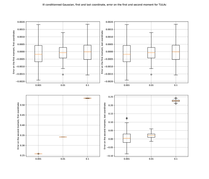
Figure 5: Boxplots of the error for TULAc on the first and second moments for the badly conditioned Gaussian variable in dimension $100$ starting at $0$ for different step sizes.

References

- [And+03] C. Andrieu, N. De Freitas, A. Doucet and M. Jordan “An introduction to MCMC for machine learning” In Machine learning 50.1-2 Springer, 2003, pp. 5–43
- [Atc06] Yves F. Atchadé “An Adaptive Version for the Metropolis Adjusted Langevin Algorithm with a Truncated Drift” In Methodology and Computing in Applied Probability 8.2, 2006, pp. 235–254 DOI: 10.1007/s11009-006-8550-0
- [BGL14] D. Bakry, I. Gentil and M. Ledoux “Analysis and geometry of Markov diffusion operators” 348, Grundlehren der Mathematischen Wissenschaften [Fundamental Principles of Mathematical Sciences] Springer, Cham, 2014, pp. xx+552 DOI: 10.1007/978-3-319-00227-9
- [BH13] N. Bou-Rabee and M. Hairer “Nonasymptotic mixing of the MALA algorithm” In IMA Journal of Numerical Analysis 33.1, 2013, pp. 80–110 DOI: 10.1093/imanum/drs003
- [BV10] Nawaf Bou-Rabee and Eric Vanden-Eijnden “Pathwise accuracy and ergodicity of metropolized integrators for SDEs” In Communications on Pure and Applied Mathematics 63.5 Wiley Subscription Services, Inc., A Wiley Company, 2010, pp. 655–696 DOI: 10.1002/cpa.20306
- [CCG12] Patrick Cattiaux, Djalil Chafaı and Arnaud Guillin “Central limit theorems for additive functionals of ergodic Markov diffusions processes” In ALEA 9.2, 2012, pp. 337–382
- [Cot+13] S.. Cotter, G.. Roberts, A.. Stuart and D. White “MCMC methods for functions: modifying old algorithms to make them faster” In Statist. Sci. 28.3, 2013, pp. 424–446 DOI: 10.1214/13-STS421
- [Dal17] Arnak S. Dalalyan “Theoretical guarantees for approximate sampling from smooth and log-concave densities” In Journal of the Royal Statistical Society: Series B (Statistical Methodology) 79.3, 2017, pp. 651–676 DOI: 10.1111/rssb.12183
- [DFG09] Randal Douc, Gersende Fort and Arnaud Guillin “Subgeometric rates of convergence of f-ergodic strong Markov processes” In Stochastic Processes and their Applications 119.3, 2009, pp. 897–923 DOI: https://doi.org/10.1016/j.spa.2008.03.007
- [DM16] A. Durmus and E. Moulines “High-dimensional Bayesian inference via the Unadjusted Langevin Algorithm” In ArXiv e-prints, 2016 arXiv:1605.01559 [math.ST]
- [DM17] Alain Durmus and Éric Moulines “Nonasymptotic convergence analysis for the unadjusted Langevin algorithm” In Ann. Appl. Probab. 27.3 The Institute of Mathematical Statistics, 2017, pp. 1551–1587 DOI: 10.1214/16-AAP1238
- [DT12] A.. Dalalyan and A.. Tsybakov “Sparse regression learning by aggregation and Langevin Monte-Carlo” In J. Comput. System Sci. 78.5, 2012, pp. 1423–1443 DOI: 10.1016/j.jcss.2011.12.023
- [Fri12] Avner Friedman “Stochastic differential equations and applications” Courier Corporation, 2012
- [GM94] U. Grenander and M.. Miller “Representations of knowledge in complex systems” With discussion and a reply by the authors In J. Roy. Statist. Soc. Ser. B 56.4, 1994, pp. 549–603 URL: http://links.jstor.org/sici?sici=0035-9246(1994)56:4%3C549:ROKICS%3E2.0.CO;2-2&origin=MSN
- [GM96] Peter W. Glynn and Sean P. Meyn “A Liapounov bound for solutions of the Poisson equation” In Ann. Probab. 24.2 The Institute of Mathematical Statistics, 1996, pp. 916–931 DOI: 10.1214/aop/1039639370
- [Gor+16] J. Gorham, A.. Duncan, S.. Vollmer and L. Mackey “Measuring Sample Quality with Diffusions” In ArXiv e-prints, 2016 arXiv:1611.06972 [stat.ML]
- [Gre83] U. Grenander “Tutorial in pattern theory” Division of Applied Mathematics, Brown University, Providence, 1983
- [GT15] David Gilbarg and Neil S Trudinger “Elliptic partial differential equations of second order” springer, 2015
- [HJ15] Martin Hutzenthaler and Arnulf Jentzen “Numerical approximations of stochastic differential equations with non-globally Lipschitz continuous coefficients” American Mathematical Society, 2015
- [HJK11] Martin Hutzenthaler, Arnulf Jentzen and Peter E. Kloeden “Strong and weak divergence in finite time of Euler’s method for stochastic differential equations with non-globally Lipschitz continuous coefficients” In Proceedings of the Royal Society of London A: Mathematical, Physical and Engineering Sciences 467.2130 The Royal Society, 2011, pp. 1563–1576 DOI: 10.1098/rspa.2010.0348
- [HJK12] Martin Hutzenthaler, Arnulf Jentzen and Peter E. Kloeden “Strong convergence of an explicit numerical method for SDEs with nonglobally Lipschitz continuous coefficients” In Ann. Appl. Probab. 22.4 The Institute of Mathematical Statistics, 2012, pp. 1611–1641 DOI: 10.1214/11-AAP803
- [HMS02] Desmond J. Higham, Xuerong Mao and Andrew M. Stuart “Strong Convergence of Euler-Type Methods for Nonlinear Stochastic Differential Equations” In SIAM Journal on Numerical Analysis 40.3, 2002, pp. 1041–1063 DOI: 10.1137/S0036142901389530
- [IW89] N. Ikeda and S. Watanabe “Stochastic Differential Equations and Diffusion Processes”, North-Holland Mathematical Library Elsevier Science, 1989
- [Kop15] Marie Kopec “Weak backward error analysis for overdamped Langevin processes” In IMA Journal of Numerical Analysis 35.2, 2015, pp. 583–614 DOI: 10.1093/imanum/dru016
- [KS91] I. Karatzas and S.E. Shreve “Brownian Motion and Stochastic Calculus”, Graduate Texts in Mathematics Springer New York, 1991
- [Kul97] S. Kullback “Information theory and statistics” Reprint of the second (1968) edition Dover Publications, Inc., Mineola, NY, 1997, pp. xvi+399
- [LFR17] S. Livingstone, M.. Faulkner and G.. Roberts “Kinetic energy choice in Hamiltonian/hybrid Monte Carlo” In ArXiv e-prints, 2017 arXiv:1706.02649 [stat.CO]
- [LMS07] H. Lamba, J.. Mattingly and A.. Stuart “An adaptive Euler–Maruyama scheme for SDEs: convergence and stability” In IMA Journal of Numerical Analysis 27.3, 2007, pp. 479–506 DOI: 10.1093/imanum/drl032
- [LS13] Robert Liptser and Albert N Shiryaev “Statistics of random Processes: I. general Theory” Springer Science & Business Media, 2013
- [LS16] Tony Lelièvre and Gabriel Stoltz “Partial differential equations and stochastic methods in molecular dynamics” In Acta Numerica 25 Cambridge University Press, 2016, pp. 681–880 DOI: 10.1017/S0962492916000039
- [MSH02] J.. Mattingly, A.. Stuart and D.. Higham “Ergodicity for SDEs and approximations: locally Lipschitz vector fields and degenerate noise” In Stochastic Process. Appl. 101.2, 2002, pp. 185–232 DOI: 10.1016/S0304-4149(02)00150-3
- [MST10] Jonathan C. Mattingly, Andrew M. Stuart and M.. Tretyakov “Convergence of Numerical Time-Averaging and Stationary Measures via Poisson Equations” In SIAM Journal on Numerical Analysis 48.2, 2010, pp. 552–577 DOI: 10.1137/090770527
- [MT93] S.. Meyn and R.. Tweedie “Stability of Markovian processes. III. Foster-Lyapunov criteria for continuous-time processes” In Adv. in Appl. Probab. 25.3, 1993, pp. 518–548 DOI: 10.2307/1427522
- [Par81] G. Parisi “Correlation functions and computer simulations” In Nuclear Physics B 180, 1981, pp. 378–384
- [PV01] E. Pardoux and Yu. Veretennikov “On the Poisson Equation and Diffusion Approximation. I” In Ann. Probab. 29.3 The Institute of Mathematical Statistics, 2001, pp. 1061–1085 DOI: 10.1214/aop/1015345596
- [RT96] G.. Roberts and R.. Tweedie “Exponential convergence of Langevin distributions and their discrete approximations” In Bernoulli 2.4, 1996, pp. 341–363 DOI: 10.2307/3318418
- [Sab13] Sotirios Sabanis “A note on tamed Euler approximations” In Electron. Commun. Probab. 18 The Institute of Mathematical Statisticsthe Bernoulli Society, 2013, pp. 10 pp. DOI: 10.1214/ECP.v18-2824
- [SV07] Daniel W Stroock and SR Srinivasa Varadhan “Multidimensional diffusion processes” Springer, 2007
- [Vil09] C. Villani “Optimal transport : old and new”, Grundlehren der mathematischen Wissenschaften Berlin: Springer, 2009 URL: http://opac.inria.fr/record=b1129524