Entropy Production and Information Flow for Markov Diffusions with Filtering

Abstract

Filtering theory gives an explicit models for the flow of information and thereby quantifies the rates of change of information supplied to and dissipated from the filter’s memory. Here we extend the analysis of Mitter and Newton [1] from linear Gaussian models to general nonlinear filters involving Markov diffusions.The rates of entropy production are now generally the average squared-field (co-metric) of various logarithmic probability densities, which may be interpreted as Fisher information associate with Gaussian perturbations (via de Bruijn’s identity). We show that the central connection is made through the Mayer-Wolf and Zakai Theorem for the rate of change of the mutual information between the filtered state and the observation history. In particular, we extend this Theorem to cover a Markov diffusion controlled by observations process, which may be interpreted as the filter acting as a Maxwell’s Dæmon applying feedback to the system.

1 Introduction

The aim of the present paper is to extend the analysis of Mitter and Newton [1] on the information flow in linear Kalman-Bucy filters to the general setting of nonlinear filters for Markov diffusion models. This leads us into the geometric setting of stochastic processes and filtering theory. In particular, the diffusion tensor defines a co-metric - introduced into Probability Theory by P.-A. Meyer and also known as the $\Gamma$-operator, or l’opérature carré du champ, see [2], or [3]. The co-metric quantifies the extent to which the generator of a diffusion process differs from a tangent vector field, and to a certain extent describes the irreversibility of the stochastic dynamics. Building on the theory of nonlinear filtering [4]-[8], we use classical results of Kadota, Zakai and Ziv [9], and of Mayer-Wolf and Zakai [10] to compute the rate of change of mutual information shared between an unknown state $X(t)$ and the observations $Y_{0}^{t}$, see also [11], [12].

We consider a system whose state, $X(t)\in\mathbb{R}^{n}$, undergoes a stochastic dynamical evolution with probability density of $X(t)$ denoted as

$$\rho_{t}(x)\equiv e^{-\Phi_{t}(x)}.$$ (1)

(More generally, we shall refer to $\Phi(x)=-\ln\rho(x)$ as being the surprise potential associated with a probability density $\rho$ for a random variable $X$. We understand that $\Phi(x)$ takes the value $+\infty$ whenever $\rho(x)=0$. The average surprise potential is then the Shannon entropy $\mathsf{H}(X)=\mathbb{E}[\Phi(X)]\equiv-\int\rho(x)\ln\rho(x)\,dx$.)

The uncertainty in the state may be measured by $\mathsf{H}_{t}=-\int\rho_{t}\ln\rho_{t}$ and should be monotonically increasing with time. In principle, we may make observations, $Y(t)$, which depend on the current state and its past history, see Figure 1.

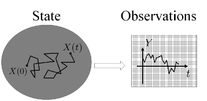
Figure 1: A randomly evolving state, $X(t)$, which is being monitored leading to partial observations $Y(t)$.

The observations may be only partial, and furthermore subject to noise. The observer may be passive, but may also alter the evolution of the system based on the observed data - that is using feedback to act as a controller, or Maxwell’s dæmon. At this stage we may flip from the pejorative view of Shannon entropy as a measure of uncertainty, to the more benign one of being a measure of information. The inverse problem of trying to guess the state $X(t)$ form the observations $Y_{0}^{t}=\{Y(s):0\leq s\leq t\}$ is a staple of signal processing: while usually not possible to completely determine the state, $X(t)$, one aims instead to construct a filter which computes the optimal estimate based on the observations, see Figure 2.

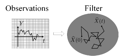
Figure 2: The estimated the state, $\widehat{X}(t)$, based on the observational data, $Y_{0}^{t}$.

In this paper, we will consider the standard problem where the state $X(t)$ undergoes a Markov diffusion and the filter computes an estimate which is optimal in the least squares sense. For an arbitrary bounded measurable function $f$, the goal is then to calculate the conditional expectation

$$\pi_{t}(f)\triangleq\mathbb{E}\big{[}f(X(t))|\mathcal{Y}_{0}^{t}\big{]},$$ (2)

where $\mathcal{Y}_{0}^{t}$ be the $\sigma$-algebra generated by the family $Y_{0}^{t}$. $\pi_{t}(f)$ is then the least-squares estimate of $f(X(t))$ given the observations. The problem is mathematically equivalent to computing the probability density valued process, $\widehat{\rho}_{t}$ [7], adapted to the filtration $\mathcal{Y}=\{\mathcal{Y}_{0}^{t}:t\geq 0\}$ such that

$$\pi_{t}(f)\equiv\int f(x)\widehat{\rho}_{t}(x,\omega)\ dx.$$ (3)

Intuitively, the flow of information to the filter should lead to a reduction in the uncertainty in the state. However, this is quantifiable.

One may further consider the effect of feedback, see [13] for discrete time and [14] for continuous time models.

1.1 Linear Gaussian Models

In this subsection we recall the results of Mitter and Newton [1] concerning the entropy production and information flow of the Kalman-Bucy filter. In this model, the processes $X$ and $Y$ are jointly Gaussian and the filter can be computed exactly.

1.1.1 Entropy Production

We consider a linear quadratic Gaussian (LQG) model where we may compute the various quantities explicitly. Here we take the SDE for the diffusion to be

$$dX\left(t\right)=AX\left(t\right)dt+BdW\left(t\right)$$ (4)

where $A\in\mathbb{R}^{n\times n}$ and $B\in\mathbb{R}^{n\times m}$, with $W$ being a canonical $m$-dimensional Wiener process. The initial condition is $X\left(0\right)\sim\mathcal{N}\left(\mu_{0},V_{0}\right)$ and one finds that $X\left(t\right)\sim\mathcal{N}\left(\mu_{t},V\left(t\right)\right)$ where the (unconditioned) mean value of $X(t)$ is

$$\mu_{t}=e^{-At}\,\mathbb{E}[X(0)],$$ (5)

and this decays to zero if $A$ is Hurwitz.

The diffusion matrix associated with problem is given by $\Sigma\equiv BB^{\top}$, which is constant in both space and time. The covariance matrix at time $t$ satisfies the differential equation

$$\frac{d}{dt}V\left(t\right)=AV\left(t\right)+V\left(t\right)A^{\top}+\Sigma,$$ (6)

with $\Sigma=BB^{\top}$ which we assume to be invertible. Under conditions that $A$ is Hurwitz, we find that there exists a steady state, $\rho_{\text{ss}}$ which is a $\mathcal{N}\left(\mu_{0},V_{\text{ss}}\right)$ distribution where the steady state covariance satisfies

$$AV_{\text{ss}}+V_{\text{ss}}A^{\top}+\Sigma=0.$$ (7)

We note that $\frac{d}{dt}V\left(t\right)=A\left(V\left(t\right)-V_{\text{ss}}\right)+\left(V\left(t\right)-V_{\text{ss}}\right)A^{\top}$.

The steady state surprise potential is then

$$\Phi_{\text{ss}}\left(x\right)\equiv\frac{1}{2}x^{\top}V_{\text{ss}}^{-1}x+E_{0}$$ (8)

where the constant is $E_{0}=\ln\left\{\sqrt{2\pi}^{n}\left|V_{\text{ss}}\right|\right\}$.

At this stage, Mitter and Newton [1] introduce a quantity

$$\mathsf{E}_{t}\triangleq\mathbb{E}[\Phi_{\text{ss}}(X(t))],$$ (9)

which plays a role similar to the free energy in thermodynamics. We will refer to it as the internal surprise at time $t$, and in the LQG case it is

$$\mathsf{E}_{t}\equiv\frac{1}{2}\int\rho_{t}\left(x\right)\text{tr}\left\{V_{\text{ss}}^{-1}xx^{\top}\right\}+E_{0}=\frac{1}{2}\text{tr}\left\{V_{\text{ss}}^{-1}V\left(t\right)\right\}+E_{0}.$$ (10)

We see that

$$\frac{d}{dt}\mathsf{E}_{t} \equiv \frac{1}{2}\text{tr}\left\{V_{\text{ss}}^{-1}\left[A\left(V\left(t\right)-V_{\text{ss}}\right)+\left(V\left(t\right)-V_{\text{ss}}\right)A^{\top}\right]\right\}$$ (11)

$$= \text{tr}\left\{V_{\text{ss}}^{-1}A\left(V\left(t\right)-V_{\text{ss}}\right)\right\}.$$

The Shannon entropy for Gaussian distributions is well known, and here we have

$$\mathsf{H}_{t}=\frac{1}{2}\ln\left|V\left(t\right)\right|+\frac{n}{2}\ln\big{(}2\pi e\big{)}.$$ (12)

and we compute its rate of change using the following Lemma.

Lemma 1

Suppose that the matrix valued function $V$ satisfies the linear differential equation $\frac{d}{dt}V\left(t\right)=AV\left(t\right)+V\left(t\right)A^{\top}+\Sigma$, (6), then

$$\frac{d}{dt}\ln|V(t)|=\text{tr}\big{\{}2A+V(t)^{-1}\Sigma\big{\}}.$$ (13)

Proof. We have the well-known identity $\frac{d}{dt}\ln|V(t)|=\text{tr}\big{\{}V(t)^{-1}\frac{dV(t)}{dt}\big{\}}$, which in this case implies $\frac{d}{dt}\ln|V(t)|=\text{tr}\big{\{}A+A^{\top}+V(t)^{-1}\Sigma\big{\}}$, where we use the commutativity under the trace. The result then follows from noting that $\text{tr}\big{\{}A\big{\}}=\text{tr}\big{\{}A^{\top}\big{\}}$.   

We therefore have that

$$\frac{d}{dt}\mathsf{H}_{t}=\text{tr}\left\{V\left(t\right)^{-1}A\left(V\left(t\right)+\frac{1}{2}\Sigma\right)\right\}\equiv\text{tr}\left\{V\left(t\right)^{-1}A\left(V\left(t\right)-V_{\text{ss}}\right)\right\},$$ (14)

where, for the last step, we substitute (7) and once again we use the invariance of the trace under commutation and transposition.

Mitter and Newton [1] then observe that the quantity analogous to the free energy, $\mathsf{F}_{t}\triangleq\mathsf{E}_{t}-\mathsf{H}_{t}$ is non-increasing. The rate of change of the $\mathsf{F}_{t}$, which we refer to as the free surprise, is given explicitly by

$$\frac{d}{dt}\mathsf{F}_{t} \equiv \text{tr}\left\{\left[V_{\text{ss}}^{-1}-V\left(t\right)^{-1}\right]A\left(V\left(t\right)-V_{\text{ss}}\right)\right\}$$ (15)

$$= -\text{tr}\left\{\left[V_{\text{ss}}^{-1}-V\left(t\right)^{-1}\right]AV_{\text{ss}}\left[V_{\text{ss}}^{-1}-V\left(t\right)^{-1}\right]V\left(t\right)\right\}$$ (16)

$$= -\frac{1}{2}\text{tr}\left\{\left[V_{\text{ss}}^{-1}-V\left(t\right)^{-1}\right]\Sigma\left[V_{\text{ss}}^{-1}-V\left(t\right)^{-1}\right]V\left(t\right)\right\}$$ (17)

from which we see that $\frac{d}{dt}\mathsf{F}_{t}\leq 0$ with equality if and only if the covariance matrix equals the steady state value.

1.1.2 The Kalman-Bucy Filter

Mitter and Newton [1] extend their analysis of entropy and information flow by considering the Kalman-Bucy filter. Here the state dynamics will be just the LQG model already presented in (4), but now take into account the information supplied by observations $Y\left(t\right)\in\mathbb{R}^{p}$ which are likewise assumed to be linear with

$$dY\left(t\right)=CX\left(t\right)dt+dU\left(t\right),$$ (18)

with $C\in\mathbb{R}^{p\times n}$ and the observational noise $U$ is taken to be independent of dynamical noise $W$ for simplicity. The initial variables $X(0)$ and $Y(0)$ are both assumed to be independent of the noises $W$ and $U$, and jointly Gaussian. The pair of processes $(X,Y)$ are then jointly Gaussian.

The conditioned probability density turns out to be again Gaussian and is given as

$$\widehat{\rho}_{t}(x,\omega)=\frac{1}{\sqrt{2\pi}^{n}|\widehat{V}_{t}|}e^{-\frac{1}{2}[x-\widehat{X}_{t}(\omega)]^{\top}\widehat{V}_{t}^{-1}[x-\widehat{X}_{t}(\omega)]},$$ (19)

where the mean $\widehat{X}_{t}(\omega)$ and covariance matrix $\widehat{V}(t)$ are explicitly computed as follows: the covariance matrix is deterministic and satisfies the Riccati equation

$$\frac{d}{dt}\widehat{V}_{t}=A\widehat{V}_{t}+\widehat{V}_{t}A^{\top}+BB^{\top}-\widehat{V}_{t}C^{\top}C\widehat{V}_{t},$$ (20)

with $\widehat{V}_{0}=Cov\left(X\left(0\right)\right)$; the mean is $\widehat{X}_{t}=\pi_{t}\left(X\right)$ and satisfies

$$d\widehat{X}_{t}=A\widehat{X}_{t}dt+\widehat{V}_{t}C^{\top}dI\left(t\right),$$ (21)

where $I$ is a stochastic process known as the innovation process

$$dY\left(t\right)=CX(t)+dU(t)\equiv C\widehat{X}_{t}\,dt+dI\left(t\right).$$ (22)

Note that we then have

$$dI\left(t\right)=C\varepsilon_{t}\left(X\right)dt+dU\left(t\right),$$

where the state error is $\varepsilon_{t}\left(X\right)=X\left(t\right)-\widehat{X}_{t}$. It is not too difficult to show that the state error satisfies

$$d\varepsilon_{t}\left(X\right)=A\varepsilon_{t}\left(X\right)dt+BdV\left(t\right)-\widehat{V}\left(t\right)C^{\top}dI\left(t\right).$$

From the point of view of filtering theory, the natural quantity to look at is the mutual information shared between the state and the observations history, $\mathsf{I}\left(X\left(t\right);Y_{0}^{t}\right)$. Mitter and Newton [1] observe the decomposition

$$\frac{d}{dt}\mathsf{I}\left(X\left(t\right);Y_{0}^{t}\right)=\dot{\mathsf{S}}(t)-\dot{\mathsf{D}}(t).$$ (23)

where the information supplied to the filter’s memory storage up to time $t$ is

$$\mathsf{S}(t)\triangleq\mathsf{I}\left(X_{0}^{t};Y_{0}^{t}\right)+\mathsf{I}\left(X(0);Y(0)\right)$$ (24)

and $\mathsf{D}(t)$ is interpreted as the information dissipated by the filter’s memory storage up to time $t$.

For the Kalman-Bucy filter, they show that

$$\frac{d}{dt}\mathsf{S}_{\text{K-B}}(t) = \frac{1}{2}\text{tr}\big{\{}C\widehat{V}(t)C^{\top}\big{\}},$$

$$\frac{d}{dt}\mathsf{D}_{\text{K-B}}(t) = \frac{1}{2}\text{tr}\big{\{}\Sigma\big{(}\widehat{V}(t)^{-1}-V(t)^{-1}\big{)}\big{\}}.$$ (25)

The rate of change of $\mathsf{S}_{\text{K-B}}(t)$ follows from a well known result of signal process due to Duncan [15], see Remark 9. We will re-derive these in Example 15.

2 Notation and Background Concepts

We recall for completeness the fundamental information theoretic and probabilistic concepts needed in this paper.

2.1 Measures of Entropy

Suppose that we have a continuous $\mathbb{R}^{n}$-valued random variable $X$ possessing a probability distribution function $\rho_{X}$, then we define the surprise function $\Phi_{X}$ by

$$\rho_{X}(x)\equiv e^{-\Phi_{X}(x)}.$$ (26)

We shall use the terms entropy and information interchangeably.

2.1.1 Shannon Entropy

The Shannon entropy of $X$ is defined to be the average surprise:

$$\mathsf{H}\left(X\right)\triangleq\mathbb{E}[\Phi_{X}]\equiv-\int\rho_{X}\ln\rho_{X}.$$ (27)

Strictly speaking the entropy is a functional of the probability distribution, $\rho_{X}$, rather than $X$ itself, but we will use this standard short hand convention throughout. If we have a family $(X_{1},\cdots,X_{n})$ of random variables on the same probability space, then we will of course understand $H(X_{1},\cdots,X_{n})$ to be their entropy of their joint distribution.

2.1.2 Relative Entropy

Let $\rho_{1}$ and $\rho_{2}$ be probability density functions on $\mathbb{R}^{n}$, then the relative entropy of $\rho_{1}$ with respect to $\rho_{2}$ is defined to be

$$\mathsf{D}\left(\rho_{1}||\rho_{2}\right)\triangleq\int\rho_{1}\ln\frac{\rho_{1}}{\rho_{2}}\equiv\mathbb{E}_{1}[\Phi_{2}-\Phi_{1}].$$ (28)

This is also known as the Kullback-Leiber divergence, the entropy of discrimination and the information distance. We note the Gibbs’ inequality $\mathsf{D}\left(\rho_{1}||\rho_{2}\right)\geq 0$ with equality if and only if $\rho_{1}=\rho_{2}$.

2.1.3 Mutual Entropy

Given a pair of random variables $X$ and $Y$ with joint density $\rho_{X,Y}$ and marginals $\rho_{X},\,\rho_{Y}$ respectively, the mutual information of $X$ and $Y$ is defined to be

$$\mathsf{I}\left(X;Y\right)\triangleq\mathsf{I}\left(Y;X\right)=\mathsf{D}\left(\rho_{X,Y}||\rho_{X}\rho_{Y}\right).$$ (29)

In detail, we have

$$\mathsf{I}\left(X;Y\right)=\int\rho_{X,Y}\ln\left[\frac{\rho_{X,Y}}{\rho_{X}\rho_{Y}}\right]\equiv\mathsf{H}\left(X\right)+\mathsf{H}\left(Y\right)-\mathsf{H}\left(X,Y\right).$$

The mutual information is the difference from the actual joint distribution to the product of the marginals. In this sense, it is a measure of the degree of correlation. As an immediate consequence of the Gibbs’ inequality, we have that the mutual information is non-negative definite, i.e. $\mathsf{I}\left(X,Y\right)\geq 0$ and we have inequality if and only if $X$ and $Y$ are independent.

2.1.4 Conditional Entropy

The conditional information of a random variable $X$ given $Y$ is defined to be

$$\mathsf{H}\left(X|Y\right)\triangleq-\int\rho_{X,Y}\ln\left[\frac{\rho_{X,Y}}{\rho_{Y}}\right]\mathsf{H}\left(X|Y\right)=\mathsf{H}\left(X,Y\right)-\mathsf{H}\left(Y\right)$$ (30)

If $X$ and $Y$ are independent, then $\mathsf{H}\left(X|Y\right)=\mathsf{H}\left(X\right)$ and $\mathsf{H}(Y|X)=\mathsf{H}(Y)$, and in particular, $\mathsf{I}(X;Y)\equiv 0$.

The mutual information satisfies the following relation:

$$\mathsf{I}\left(X;Y\right) = \mathsf{H}\left(X\right)-\mathsf{H}\left(X|Y\right).$$ (31)

2.1.5 Fisher Entropy

A final form of entropy that will be of relevance to use is the Fisher information, specifically the translation Fisher information we recall below. Let $\{\rho_{X}^{\theta}:\theta\in\Theta\}$ be a family of probability density functions for a random variable $X$ parametrized by a parameter taking values in an open subset $\Theta$ of $\mathbb{R}^{p}$. We say that $\theta\mapsto\rho_{X}^{\theta}\left(x\right)$ is the likelihood of $\theta$ given the observation $x$. The score is defined to be the random vector in $\mathbb{R}^{p}$ with components

$$s_{i}^{\theta}\left(X\right)\triangleq\frac{\partial}{\partial\theta_{i}}\ln\rho_{X}^{\theta}.$$ (32)

It is easy to see that $\mathbb{E}_{\theta}\left[s_{i}^{\theta}\left(X\right)\right]\equiv 0$. The Fisher information is the $p\times p$ matrix with entries

$$\mathsf{F}_{ij}^{\theta}\left(X\right)\triangleq\mathbb{E}_{\theta}\left[s_{i}^{\theta}\left(X\right)s_{j}^{\theta}\left(X\right)\right].$$ (33)

In other words, the Fisher information is the covariance matrix for the score variable. In detail, we have

$$\mathsf{F}_{ij}^{\theta}\left(X\right)=\int\rho_{X}^{\theta}\left(\frac{\partial}{\partial\theta_{i}}\ln\rho_{X}^{\theta}\right)\left(\frac{\partial}{\partial\theta_{j}}\ln\rho_{X}^{\theta}\right).$$

Let us suppose that we know that the distribution of a random $n$-vector is known up to translation. That is, we have a fixed distribution $\rho$ and the actual distribution is of the form

$$\rho^{\theta}\left(x\right)=\rho\left(x-\theta\right)$$

where $\theta\in\mathbb{R}^{n}$ is unknown parameter. In this case the score is $s^{\theta}\left(X\right)=\nabla_{\theta}\ln\rho\left(x-\theta\right)$ but this can be equivalently written as $-\nabla_{x}\ln\rho\left(x-\theta\right)$. We shall refer to the associated Fisher information matrix in this case as the translational Fisher information, and denote it by $\mathsf{J}(X)$. It takes the form

$$\mathsf{F}_{ij}^{\theta}\left(X\right)=\mathsf{J}_{ij}\left(X\right)\triangleq\int\rho\left(x-\theta\right)s_{i}^{\theta}\left(X\right)s_{j}^{\theta}\left(X\right)\,dx$$

however we can perform the volume preserving change of variable $x^{\prime}=x-\theta$ to get the simplified form

$$\mathsf{J}_{ij}\left(X\right) = \int\rho\frac{\partial\ln\rho}{\partial x_{i}}\frac{\partial\ln\rho}{\partial x_{j}}.$$ (34)

We also have $\mathsf{J}_{ij}\left(X\right)\equiv\int\frac{1}{\rho}\frac{\partial\rho}{\partial x_{i}}\frac{\partial\rho}{\partial x_{j}}\equiv-\int\rho\frac{\partial^{2}}{\partial x_{i}\partial x_{j}}\ln\rho$. Note that this Fisher information does not depend on the value $\theta$, only on the representative distribution $\rho$. We also note the rescaling law $\mathsf{J}\left(aX+b\right)=\frac{1}{a^{2}}\mathsf{J}\left(X\right)$. The well-known Cramér-Rao inequality is equivalent to $Cov\left(X\right)\geq\mathsf{J}\left(X\right)^{-1}$.

An important connection between Shannon and Fisher information arises in the context of Gaussian perturbations. We have, for instance, De Bruijn’s Identity which states that if $X$ is a random $n$-vector and $Z$ be a standard Gaussian $n$-vector independent of $X$, then

$$\frac{d}{dt}\mathsf{H}\left(X+\sqrt{t}Z\right)=\frac{1}{2}\mathrm{tr}\mathsf{J}\left(X+\sqrt{t}Z\right).$$ (35)

We also note the log-Sobolev inequality for Fisher information. Let $X$ be a random $n$-vector and suppose that $\mathsf{J}\left(X+\sqrt{t}Z\right)$ exists and is differentiable in $t$ in a neighborhood of 0 for arbitrary standard Gaussian $n$-vector perturbations $Z$ independent of $X$. Then

$$\left.\frac{d}{dt}\frac{n}{\mathsf{J}\left(X+\sqrt{t}Z\right)}\right|_{t=0}\geq 1.$$ (36)

2.2 Stochastic Dilations

We fix a probability space $\left(\Omega,\mathcal{A},\mathbb{P}\right)$. Let $\mathcal{F}=\left\{\mathcal{F}_{0}^{t}\right\}_{t\geq 0}$ be a filtration on a sample space $\Omega$, that is, an increasing and right-continuous family of $\sigma$-subalgebras of $\mathcal{A}$, with each $\mathcal{F}_{0}^{t}$ containing all sets of measure zero. As usual, we say that a process $X=\left\{X\left(t\right)\right\}_{t\geq 0}$ is $\mathcal{F}$-adapted if $X\left(t\right)$ is $\mathcal{F}_{0}^{t}$-measurable for each $t\geq 0$. We say that $M$ is a martingale wrt. the filtration if it is an integrable process such that $\mathbb{E}\left[M\left(t\right)|\mathcal{F}_{0}^{s}\right]\equiv M\left(s\right)$ for all $0\leq s\leq t$.

More generally, if $X$ is a stochastic process, we define its conditional derivative wrt. the filtration as

$$\mathbb{D}_{\mathcal{F}}X\left(t\right)\triangleq\lim_{\tau\rightarrow 0^{+}}\mathbb{E}[\frac{X\left(t+\tau\right)-X\left(t\right)}{\tau}\mid\mathcal{F}_{0}^{t}].$$ (37)

We may refer to $\mathbb{D}_{\mathcal{F}}X\left(t\right)$ as the conditional velocity wrt. the filtration. Martingales are then processes with zero conditional velocity (or, equivalently, vanishing trend). For a pair of processes $X$ and $Y$, we define their angular bracket wrt. the filtration as

$$\left\langle X,Y\right\rangle_{t,\mathcal{F}}\triangleq\int_{0}^{t}\mathbb{E}\left[dX\left(s\right)dY\left(s\right)|\mathcal{F}_{0}^{s}\right]ds.$$ (38)

Given an operator $\mathcal{L}$ from the smooth functions $\mathscr{C}^{\infty}(\mathbb{R}^{n})$ to the bounded continuous function on $\mathbb{R}^{n}$, then an $\mathbb{R}^{n}$-valued process, $X$, is said to solve the martingale problem associated with $\mathcal{L}$ if, for each $f\in\mathscr{C}^{\infty}(\mathbb{R}^{n})$, the equation

$$f\left(X\left(t\right)\right)=f\left(X\left(0\right)\right)+\int_{0}^{t}\mathcal{L}f\,\left(X\left(s\right)\right)ds+M_{f}\left(t\right)$$ (39)

defines a martingale process $M_{f}$.

In the following we will be interested in with diffusion processes on $\mathbb{R}^{n}$, where the associated operator $\mathcal{L}$ is elliptic. Here we have

$$\mathbb{D}_{\mathcal{F}}f(X\left(t\right))\equiv\mathcal{L}f(X\left(t\right))$$ (40)

and the angular bracket takes the form

$$\frac{d}{dt}\left\langle f\left(X\right),g\left(X\right)\right\rangle_{t,\mathcal{F}}\equiv\left.2\Gamma_{\mathcal{L}}\left(f,g\right)\right|_{X\left(t\right)}$$ (41)

where the co-metric is defined to be

$$\Gamma_{\mathcal{L}}\left(f,g\right)\triangleq\mathcal{L}\left(fg\right)-\left(\mathcal{L}f\right)g-f\left(\mathcal{L}g\right).$$ (42)

The co-metric quantifies the obstruction to $\mathcal{L}$ being a tangent vector field since $\Gamma_{\mathcal{L}}\left(f,g\right)\equiv 0$ for $\mathcal{L}=v^{i}\left(x\right)\partial_{i}$. It has the following properties:

1. $\Gamma_{\mathcal{L}+\mathcal{K}}=\Gamma_{\mathcal{L}}+\Gamma_{\mathcal{K}}$;

2. it is symmetric $\Gamma_{\mathcal{L}}\left(f,g\right)=\Gamma_{\mathcal{L}}\left(g,f\right)$;

3. off-diagonal terms are determined through polarization:

   $$2\Gamma_{\mathcal{L}}\left(f,g\right)=\Gamma_{\mathcal{L}}\left(f+g,f+g\right)-\Gamma_{\mathcal{L}}\left(f-g,f-g\right).$$ (43)

The following is easily verified.

Proposition 2

Let $\mathcal{K}f=\alpha f+\beta^{i}f_{,i}+\frac{1}{2}\gamma^{ij}f_{,ij}$, for functions $\alpha,\beta^{i}$ and $\gamma^{ij}=\gamma^{ji}$, then

$$\Gamma_{\mathcal{K}}\left(f,g\right)=-\alpha fg+\gamma^{ij}f_{,i}g_{,j}.$$ (44)

We remark that there is an analogue of the Ricci Tensor due to Bakry-Emery tensor $\Gamma_{\mathcal{L}}^{2}\left(f,g\right)\triangleq\mathcal{L}\left(\Gamma_{\mathcal{L}}\left(f,g\right)\right)-\Gamma_{\mathcal{L}}\left(\mathcal{L}f,g\right)\ -\Gamma_{\mathcal{L}}\left(f,\mathcal{L}g\right)$, see for instance [3]. We should remark that Bakry and Emery have developed a theory on inequalities based on their $\Gamma^{2}$ tensor which generalize the log-Sobolev inequality (36).

We note that we have $\frac{d}{dt}\mathbb{E}\left[f\left(X\left(t\right)\right)\right]=\mathbb{E}\left[\mathcal{L}f\,\left(X\left(t\right)\right)\right]$. If define the probability density $\rho_{t}$ for $X\left(t\right)$, so that

$$\mathbb{E}\left[f\left(X\left(t\right)\right)\right]\equiv\int f\left(x\right)\rho_{t}\left(x\right)dx$$ (45)

then the density satisfies the Fokker-Planck equation

$$\frac{\partial}{\partial t}\rho_{t}=\mathcal{L}^{\star}\rho_{t}$$ (46)

where the adjoint operator is defined by the duality

$$\int\mathcal{L}f\left(x\right)\rho\left(x\right)dx=\int f\left(x\right)\mathcal{L}^{\star}\rho\left(x\right)dx.$$ (47)

3 Entropy Production For Markov Diffusions

3.1 Markov Diffusions

Let us specialize to a state process, $X$, which is diffusion on $\mathbb{R}^{n}$ satisfying a stochastic differential equation of the form

$$dX^{i}\left(t\right)=v^{i}\left(X\left(t\right)\right)dt+\sum_{\alpha=1}^{r}B_{\alpha}^{i}\left(X\left(t\right)\right)dW^{\alpha}\left(t\right)$$ (48)

where $W=\left(W^{1},\cdots,W^{r}\right)$ is an $r$-dimensional Wiener process (the dynamical noise). The associated operator is then

$$\mathcal{L}=v^{i}\left(x\right)\partial_{i}+\frac{1}{2}\Sigma^{ij}\left(x\right)\partial_{ij},$$ (49)

where the diffusion tensor field is

$$\Sigma^{ij}\left(x\right)=\sum_{\alpha}B_{\alpha}^{i}\left(x\right)B_{\alpha}^{j}\left(x\right).$$ (50)

The diffusion tensor, $\Sigma$, then turns out to be the co-metric tensor as we have

$$\Gamma_{\mathcal{L}}\left(f,g\right)\equiv\sum_{\alpha}B_{\alpha}\left(f\right)B_{\alpha}\left(g\right)=\Sigma^{ij}f_{,i}g_{,j}=\left(\nabla f\right)^{\top}\Sigma\left(\nabla g\right)$$ (51)

where we have the $r$ tangent vector fields $B_{\alpha}$ with $B_{\alpha}\left(f\right)=B_{\alpha}^{i}\left(x\right)\,\left(\partial_{i}f\right)$. The adjoint generator is now given by

$$\mathcal{L}^{\star}\rho\equiv-\sum_{i}\partial_{i}\left(\rho v^{i}\right)+\frac{1}{2}\sum_{i,j}\partial_{ij}^{2}\left(\Sigma^{ij}\rho\right).$$ (52)

A general feature of Markov diffusions is that we now have the additional properties:

1. it is a bi-derivation: $\Gamma_{\mathcal{L}}\left(f,gh\right)=\Gamma_{\mathcal{L}}\left(f,g\right)h+g\Gamma_{\mathcal{L}}\left(f,h\right)$;

2. it is positive semi-definite: $\Gamma_{\mathcal{L}}\left(f,f\right)\geq 0$.;

Lemma 3

The Fokker-Planck equation is equivalent to the continuity equation

$$\frac{\partial\rho_{t}}{\partial t}+\nabla.J_{t}=0$$ (53)

where the probability flux density $J_{t}$ has the components

$$J^{i}\left(x,t\right)=v^{i}\left(x\right)\rho_{t}\left(x\right)-\frac{1}{2}\frac{\partial}{\partial x^{j}}\left(\Sigma^{ij}\left(x\right)\rho_{t}\left(x\right)\right).$$ (54)

We remark that the flux may also be written in the form

$$J_{t}=\rho_{t}u-\frac{1}{2}\Sigma\nabla\rho_{t},$$ (55)

where we introduce a new velocity field $u$ having the components

$$u^{i}\triangleq v^{i}-\frac{1}{2}\frac{\partial\Sigma^{ij}}{\partial x^{j}}.$$ (56)

Let us remark that the dual generator may be written in terms of the new velocity $u$ as

$$\mathcal{L}^{\star}f=-\nabla.\left(uf\right)+\frac{1}{2}\Sigma^{ij}f_{,ij},$$ (57)

and in particular

$$\mathcal{L}^{\star}1=-(\nabla.u).$$ (58)

If, moreover, $\rho_{t}(x)$ is strictly positive for all $x$ and $t\geq 0$, then we may write the flux as

$$J_{t}=\rho_{t}\left[u-\frac{1}{2}\Sigma\,\left(\nabla\ln\rho_{t}\right)\right].$$ (59)

In this case we can write $\rho_{t}(x)\equiv e^{-\Phi_{t}(x)}$, where $\Phi_{t}$ may be referred to as the surprise potential. As $\Phi_{t}=-\ln\rho_{t}$, we see that

$$J_{t}\equiv\rho_{t}\left[u-\frac{1}{2}\Sigma\,\left(\nabla\ln\rho_{t}\right)\right]=\rho_{t}\left[u+\frac{1}{2}\Sigma\,\left(\nabla\Phi_{t}\right)\right]$$ (60)

Definition 4

We say that the Markov diffusion admits a steady state it there is probability density, $\rho_{\text{ss}}\left(x\right)$, such that $\mathcal{L}^{\star}\rho_{\text{ss}}\equiv 0$.

If a steady state exists, then the Fokker-Planck equation tells us that it is invariant and we see that the flux should vanish for this state leaving

$$u\left(x\right)=\frac{1}{2}\Sigma\left(x\right)\,\nabla\ln\rho_{\text{ss}}\left(x\right)=-\frac{1}{2}\Sigma\left(x\right)\,\nabla\Phi_{\text{ss}}\left(x\right).$$ (61)

If we further assume that the steady state is strictly positive then we may likewise introduce a steady state surprise potential function $\Phi_{\text{ss}}\left(x\right)=-\ln\rho_{\text{ss}}\left(x\right)$. Note that we may write

$$J_{t} = \frac{1}{2}\rho_{t}\Sigma\,\nabla\left(\Phi_{t}-\Phi_{\text{ss}}\right)=-\frac{1}{2}\rho_{t}\Sigma\,\left(\nabla\ln\frac{\rho_{t}}{\rho_{\text{ss}}}\right).$$ (62)

3.2 Entropy Production for General Diffusions

The entropy may be interpreted as the uncertainty, and for diffusions one would expect the entropy associated with the diffusing variable $X(t)$ to increase as $t$ increases. Not least because we are continuously injecting more noise into the dynamics. Indeed, we have a continuous Gaussian perturbation. We will compute the rate of change of the entropy $\mathsf{H_{t}}=\mathsf{H}\left(X(t)\right)$ associated with the probability density $\rho_{t}$ of the diffusion (48) in this section. We begin, however, with the deterministic case.

Suppose that we have a deterministic flow generated by a velocity vector field $v=v^{i}\left(x\right)\partial_{i}$. The dynamics is then given by the system of ODEs $\frac{d}{dt}X^{i}\left(t\right)=v^{i}\left(X\left(t\right)\right)$. In this case, the Fokker-Planck equation reduces to the continuity equation with the simplified flux $J_{t}\left(x\right)=v\left(x\right)\rho_{t}\left(x\right)$. We then have

$$\frac{d}{dt}\mathsf{H}\left(X\left(t\right)\right) = -\frac{d}{dt}\int\rho_{t}\ln\rho_{t}=-\int\left(1+\ln\rho_{t}\right)\frac{\partial\rho_{t}}{\partial t}=\int\left(1+\ln\rho_{t}\right)\nabla\left(\rho_{t}v\right)$$ (63)

$$= -\int\left(\nabla\ln\rho_{t}\right)^{\top}\rho_{t}v=-\int\left(\nabla\rho_{t}\right)^{\top}v=\int\rho_{t}\nabla.v.$$

In other words,

$$\frac{d}{dt}\mathsf{H}\left(X\left(t\right)\right)=\mathbb{E}\left[\left.\left(\nabla.v\right)\right|_{X\left(t\right)}\right].$$ (64)

The rate of production of entropy is therefore the average of the divergence of the velocity field. This makes intuitive sense as $\nabla.v$ measures the local change of volume, so its average gives a global measure of change in uncertainty. In the special case of an incompressible fluid $\left(\nabla.v\equiv 0\right)$ we have zero entropy production - this includes Hamiltonian systems by virtue of Liouville’s Theorem.

Now let us treat the diffusive case.

Lemma 5

Let $f$ be a strictly positive twice continuously differentiable function, then for a Markov diffusion generator, $\mathcal{L}$,

$$\mathcal{L}\ln f=\frac{1}{f}\mathcal{L}f-\frac{1}{2}\Gamma_{\mathcal{L}}\left(\ln f,\ln f\right).$$ (65)

Proof. This is actually a straightforward derivation:

$$\mathcal{L}\ln f = \frac{1}{f}v^{\top}\nabla f+\frac{1}{2}\Sigma^{ij}\left(\frac{1}{f}f_{,ij}-\frac{1}{f^{2}}f_{,i}f_{,j}\right)$$ (66)

$$= \frac{1}{f}\mathcal{L}f-\frac{1}{2f^{2}}\Gamma_{\mathcal{L}}\left(f,f\right)=\frac{1}{f}\mathcal{L}f-\frac{1}{2}\Gamma_{\mathcal{L}}\left(\ln f,\ln f\right).$$ (67)

 

Theorem 6

The entropy production rate for a diffusion process $X\left(t\right)$ is given by

$$\frac{d}{dt}\mathsf{H}\left(X\left(t\right)\right)=\mathbb{E}\left[\left.\left(\nabla.u\right)\right|_{X\left(t\right)}+\left.\frac{1}{2}\Gamma_{\mathcal{L}}\left(\ln\rho_{t},\ln\rho_{t}\right)\right|_{X\left(t\right)}\right].$$ (68)

Proof. We now have

$$\frac{d}{dt}\mathsf{H}\left(X\left(t\right)\right) = -\int\left(1+\ln\rho_{t}\right)\frac{\partial\rho_{t}}{\partial t}$$

$$=-\int\left(1+\ln\rho_{t}\right)\mathcal{L}^{\star}\rho_{t}=-\int\left(\mathcal{L}\ln\rho_{t}\right)\rho_{t}$$

but, from Lemma 5, $\mathcal{L}\ln\rho_{t}=\frac{1}{\rho_{t}}\mathcal{L}\rho_{t}-\frac{1}{2}\Gamma_{\mathcal{L}}\left(\ln\rho_{t},\ln\rho_{t}\right)$.

Therefore,

$$\frac{d}{dt}\mathsf{H}\left(X\left(t\right)\right)=\int\left(-\mathcal{L}\rho_{t}+\frac{1}{2}\rho_{t}\Gamma_{\mathcal{L}}\left(\ln\rho_{t},\ln\rho_{t}\right)\right).$$

The first term here is $-\int\left(\mathcal{L}\rho_{t}\right)=-\int\rho_{t}\mathcal{L}^{\star}1=\int\rho_{t}\nabla.u$, and this observation leads to the desired result.   

Note that this says that the entropy rate consists of a geometric dilation term (similar to the deterministic case, but now with the divergence of $u$ instead of $v$) and an additional term which is irreversible in the sense that it comes from the second-order terms of the generator.

We remark that Theorem 6 may be proved more directly from the Fokker-Planck equation and an integration by parts,

$$\frac{d}{dt}\mathsf{H}_{t} = \int\left(1+\ln\rho_{t}\right)\left(\nabla.J\right)$$

$$= -\int\left(\nabla\ln\rho_{t}\right)^{\top}J$$

$$= -\int\rho_{t}u^{\top}\left(\nabla\ln\rho_{t}\right)+\frac{1}{2}\int\rho_{t}\left(\nabla\ln\rho_{t}\right)^{\top}\Sigma\left(\nabla\ln\rho_{t}\right)$$

and the last step follows directly by substituting in (60) to eliminate $J_{t}$. The last term is readily shown to be $\int\rho_{t}\left(\nabla.u\right)$ by a simple integration by parts. This proof is very much related to the textbook proof of the de Bruijn identity, equation (35), where the Gaussian perturbation is viewed as convolution wrt. the fundamental solution to the heat equation (the Wiener kernel!) and similarly employing the integration by parts step.

Another point of interest is that the term in (68) involving the $\Gamma$-operator of the generator with the score (logarithmic derivative) as argument is evidently a form of Fisher information. In fact, it reduces to $\text{tr}\,\mathsf{J}\left(X(t)\right)$ in the special case where $\Sigma$ is the identity matrix. One can, in fact, show that if the diffusion matrix $\Sigma$ is invertible and $\rho_{t}$ is strictly positive, then the equation (68) may be written as

$$\frac{d}{dt}\mathsf{H}_{t}=2\int\frac{1}{\rho_{t}}J_{t}^{\top}\Sigma^{-1}J_{t}-2\int u^{\top}\Sigma^{-1}J_{t}.$$ (69)

We can now give the appropriate extension of the Mitter-Newton entropy production equations for Markov diffusions with a steady state.

Definition 7

Suppose that a Markov diffusion $X(t)$ admits a strictly positive, steady state $\rho_{\text{ss}}\equiv e^{-\Phi_{\text{ss}}}$ The free surprise associated with the diffusion is defined to be the relative entropy

$$\mathsf{F}_{t}\triangleq\mathsf{D}\left(\rho_{t}||\rho_{\text{ss}}\right).$$ (70)

The internal surprise associated with the diffusion $X(t)$ is defined to be

$$\mathsf{E}_{t}\triangleq\mathbb{E}\left[\Phi\left(X(t)\right)\right].$$ (71)

We note that

$$\mathsf{F}_{t}=\int\rho_{t}\ln\frac{\rho_{t}}{\rho_{\text{ss}}}=\int\rho_{t}\ln\rho_{t}-\int\rho_{t}\ln\rho_{\text{ss}},$$ (72)

and so the free surprise, internal surprise and entropy, associated with a diffusion $X(t)$ with steady state $\rho_{\text{ss}}$, are related by

$$\mathsf{F}_{t}=\mathsf{E}_{t}-\mathsf{H}_{t}.$$ (73)

We again have the clear analogy with thermodynamics that was the central motivation of Mitter and Newton [1]. The free and internal surprises correspond to the free and internal energies, while the information is the entropy - the relation (73) is then the standard thermodynamic relation with unit temperature. The free surprise is non-increasing and its rate of change involves the co-metric.

Theorem 8

Let $\left\{X\left(t\right)\right\}_{t\geq 0}$ be the diffusion process satisfying the stochastic differential equation (48) and assume that the diffusion matrix $\Sigma$ is everywhere invertible and that there exists a unique steady state $\rho_{\text{ss}}$. Then the associated free surprise is non-increasing, and we have

$$\frac{d}{dt}\mathsf{F}_{t}=-\frac{1}{2}\mathbb{E}\left[\left.\Gamma_{\mathcal{L}}\left(\ln\frac{\rho_{t}}{\rho_{\text{ss}}},\ln\frac{\rho_{t}}{\rho_{\text{ss}}}\right)\right|_{X\left(t\right)}\right]\leq 0.$$ (74)

Proof. We have

$$\mathsf{F}_{t} = \int(1+\ln\rho_{t}-\ln\rho_{\text{ss}})\frac{\partial\rho_{t}}{\partial t}$$

$$= \int(1+\ln\rho_{t}-\ln\rho_{\text{ss}})\mathcal{L}^{\star}\rho_{t}$$

$$= \int\left(\mathcal{L}\ln\frac{\rho_{t}}{\rho_{\text{ss}}}\right)\rho_{t}$$

$$= \int\left[\frac{\rho_{ss}}{\rho_{t}}\left(\mathcal{L}\frac{\rho_{t}}{\rho_{\text{ss}}}\right)-\frac{1}{2}\Gamma_{\mathcal{L}}\left(\ln\frac{\rho_{t}}{\rho_{\text{ss}}},\ln\frac{\rho_{t}}{\rho_{\text{ss}}}\right)\right]\rho_{t}$$

where we used Lemma 5. The first of these terms vanishes as it equals

$$\int\rho_{\text{ss}}\left(\mathcal{L}\frac{\rho_{t}}{\rho_{\text{ss}}}\right)=\int\left(\mathcal{L}^{\star}\rho_{\text{ss}}\right)\frac{\rho_{t}}{\rho_{\text{ss}}}=0,$$

since $\mathcal{L}^{\star}\rho_{\text{ss}}\equiv 0$ for a steady state.   

We remark that if $\rho_{t}$ is strictly positive, and if $\Sigma$ is everywhere invertible, then the (74) is equivalent to

$$\frac{d}{dt}\mathsf{F}_{t}=-\frac{1}{2}\int\frac{1}{\rho_{t}}J_{t}^{\top}\Sigma^{-1}J_{t}\leq 0.$$ (75)

This may be alternatively proved by noting that $\frac{d}{dt}\mathsf{F}_{t}=\frac{d}{dt}\mathsf{E}_{t}-\frac{d}{dt}\mathsf{H}_{t}$. The rate of change of the internal surprise is

$$\frac{d}{dt}\mathsf{E}_{t} = \frac{d}{dt}\int\rho_{t}\left(x\right)\Phi_{\text{ss}}\left(x\right)=\int\frac{\partial\rho_{t}\left(x\right)}{\partial t}\Phi_{\text{ss}}\left(x\right)$$ (76)

$$= -\int\left(\nabla.J_{t}\right)^{\top}\Phi_{\text{ss}}=\int J_{t}^{\top}\nabla\Phi_{\text{ss}}=-2\int J_{t}^{\top}\Sigma u,$$ (77)

where we used the Fokker-Planck equation, integration by parts, and for the last step (61). The term $\frac{d}{dt}\mathsf{E}_{t}$ therefore corresponds to the second term in (69) which now reads as $\frac{d}{dt}\mathsf{H}_{t}=\frac{1}{2}\int\frac{1}{\rho_{t}}J_{t}^{\top}\Sigma^{-1}J_{t}+\frac{d}{dt}\mathsf{E}_{t}$, and this gives the desired result.

4 Filtering & Entropy Reduction

The filtering problem considered here is the following standard one. We have a diffusion process, $X$, on $\mathbb{R}^{n}$ and make observations leading to an $\mathbb{R}^{p}$-valued process $Y$. Denoting the $\sigma$-algebra generated by the observations over the time interval $\left[0,t\right]$ by $\mathcal{Y}_{0}^{t}$, we wish to compute the filtered estimate $\pi_{t}\left(f\right)\triangleq\mathbb{E}\left[f\left(X\left(t\right)\right)|\mathcal{Y}_{0}^{t}\right]$. Equivalently, we may compute the $\mathcal{Y}$-adapted probability density valued process $\widehat{\rho}$ such that $\pi_{t}\left(f\right)\equiv\int f\left(x\right)\widehat{\rho}_{t}\left(x\right)dx$. We refer to $\widehat{\rho}_{t}$ as the conditioned density and recall that $\mathbb{E}\left[\widehat{\rho}_{t}\right]\equiv\rho_{t}$.

Let us suppose that the observations satisfy

$$dY\left(t\right)=H\left(t\right)dt+dU\left(t\right)$$ (78)

where $H$ is an $\mathbb{R}^{p}$-valued process adapted to the filtration generated by $X$, and $U$ is a $p$-dimensional Wiener process independent of $X$. We encounter the drift term $H\left(t\right)\equiv\mathbb{D}_{\mathcal{U}}H\left(t\right)$, where $\mathcal{U}$ is the filtration generated by the observational noise $U$. However, as we only observe $Y$ it makes more sense to introduce the new process

$$\widehat{H}\left(t\right)\triangleq\mathbb{D}_{\mathcal{Y}}Y\left(t\right).$$ (79)

A Theorem of Duncan [15] states that the mutual information shared between the signal $H_{0}^{t}$ and the observations $Y_{0}^{i}$ is given by

$$\mathsf{I}\left(H_{0}^{t};Y_{0}^{t}\right)=\frac{1}{2}\int_{0}^{t}\mathbb{E}\left[\left|\varepsilon\left(H,s\right)\right|^{2}ds\right]$$ (80)

where the estimation error is

$$\varepsilon\left(H,t\right)=H\left(t\right)-\widehat{H}\left(t\right),$$ (81)

or equivalently, $\left(\mathbb{D}_{\mathcal{U}}-\mathbb{D}_{\mathcal{Y}}\right)Y\left(t\right)$. The proof makes extensive use of Girsanov transformations [16].

Remark 9

Duncan’s Theorem takes a simple form for the Kalman-Bucy filter. As $H(t)=CX(t)$, we see that $\varepsilon(H,t)\equiv C\varepsilon_{t}(X)$ where $\varepsilon_{t}(X)$ is the state error. Therefore, $\mathbb{E}\left[\left|e(H,\tau)\right|^{2}\right]=\text{tr}\,\left\{C^{\top}C\widehat{V}(\tau)\right\}$and therefore the mutual information is

$$\mathsf{I}_{\text{K-B}}\left(Y_{0}^{t};X_{0}^{t}\right)=\frac{1}{2}\int_{0}^{t}\text{tr}\left\{C\widehat{V}\left(\tau\right)C^{\top}\right\}d\tau.$$ (82)

We may also write

$$dY\left(t\right)\equiv\widehat{H}(t)\,dt+dI\left(t\right)$$ (83)

where the innovations process $\left\{I\left(t\right)\right\}_{t\geq 0}$ is defined as

$$dI\left(t\right) \triangleq dY\left(t\right)-\widehat{H}(t)\,dt$$ (84)

$$\equiv dU\left(t\right)+\varepsilon\left(H,t\right)\,dt.$$

The increment $dI\left(t\right)$ is the difference between the observed signal, $dY\left(t\right)$, and what we would have expected, $\widehat{H}(t)\,dt$, given the observations up to time.

The innovations process is a martingale wrt. the filtration $\left\{\mathcal{Y}_{0}^{t}\right\}_{t\geq 0}$, and furthermore we have $\left(dI\right)^{2}=\left(dU\right)^{2}=dt$ so by Lévy’s Theorem it is a Wiener process with respect to this filtration.

4.1 Filtering Markov Diffusions

We consider the problem of a system with unobserved state $X(t)$ in $\mathbb{R}^{n}$. We assume that it evolves according to the stochastic differential equation (48) which we write in the vector form

$$(\text{State Dynamics})\qquad dX(t)=v\left(X(t)\right)dt+B\left(X(t)\right)dW(t),$$ (85)

with $W$ an $r$-dimensional canonical Wiener process, as before.

Information about the state comes from an observation process in $\mathbb{R}^{p}$

$$(\text{Observations)}\qquad\qquad\qquad dY(t)=h\left(X(t)\right)dt+dU(t),$$ (86)

or $dY^{i}(t)=h^{i}\left(X(t)\right)dt+dU^{i}(t)$ in component form. Again we assume that $U$ is a $p$-dimensional Wiener process. The dynamical noise $W$ is assumed to be statistically independent of the observational noise $U$ corrupting observed signals. We shall denote by $\mathcal{Y}_{0}^{t}$ the $\sigma$-algebra generated by the observations $\{Y(s):0\leq s\leq t\}$. To initialize the problem, we may fix a probability measure $\mathbb{P}_{X(0),Y(0)}$ for the initial state and observation.

The filter for the problem (85, 86) can be written as

$$\pi_{t}\left(f\right)\equiv\frac{\sigma_{t}\left(f\right)}{\sigma_{t}\left(1\right)}$$ (87)

where $\sigma_{t}(f)$ as the unnormalized filter, or the Zakai filter. The normalization $\sigma_{t}(1)$ will be a stochastic process adapted to the filtration of $Y$. The process $\sigma_{t}(f)$ satisfies the Zakai equation

$$d\sigma_{t}\left(f\right) = \sigma_{t}\left(\mathcal{L}f\right)dt+\sigma_{t}(fh^{\top})\,dY(t),$$ (88)

where $\mathcal{L}$ is the generator of the diffusion $X$. The normalization process $\sigma_{t}\left(1\right)$ is given by

$$\sigma_{t}\left(1\right)=\exp\left\{\int_{0}^{t}\pi_{s}\left(h\right)^{\top}dY\left(s\right)-\frac{1}{2}\int_{0}^{t}|\pi_{s}\left(h\right)|^{2}ds\right\},$$ (89)

and, in particular,

$$\mathbb{E}\left[\ln\sigma_{t}\left(1\right)\right]=\frac{1}{2}\int_{0}^{t}\mathbb{E}\left[|\pi_{s}\left(h\right)|^{2}\right]ds.$$ (90)

From the Zakai filter, we may deduce the form of the normalized filter $\pi_{t}(f)$.

Theorem 10 (Kushner-Stratonovich)

The filter $\pi_{t}(f)$ satisfies the equation

$$d\pi_{t}(f)=\pi_{t}\left(\mathcal{L}f\right)dt+\left[\pi_{t}(fh^{\top})-\pi_{t}\left(f\right)\pi_{t}(h^{\top})\right]\,dI(t),$$ (91)

known as the Kushner-Stratonovich equation, where $\{I(t):t\geq 0\}$ is the innovations process:

$$dI(t)\triangleq dY(t)-\pi_{t}\left(h\right)dt.$$ (92)

For completeness, we give a derivation of the Kushner-Stratonovich equation, (91), in in Section 8.1. We say that the filtering problem admits a conditional density $\widehat{\rho}_{t}$ if we have

$$\widehat{f}_{t}(\omega)=\int f(x)\widehat{\rho}_{t}(x,\omega)dx.$$ (93)

In this case the Kushner-Stratonovich equation is equivalent to

$$d\widehat{\rho}_{t}(x,\omega) = \mathcal{L}^{\star}\widehat{\rho}_{t}(x,\omega)\,dt$$

$$+\widehat{\rho}_{t}(x,\omega)\,\left\{h^{\top}(x)-\int h(x^{\prime})^{\top}\widehat{\rho}_{t}(x^{\prime},\omega)dx^{\prime}\right\}\,dI(t,\omega).$$

Note that this is nonlinear in $\widehat{\rho}_{t}$.

If we average over all outputs we get an average density $\rho_{t}$ which is just the unconditional density for the diffusion $X$, and which satisfies the Fokker-Planck (Kolmogorov forward) equation, $\frac{d}{dt}\rho_{t}=\mathcal{L}^{\star}\rho_{t}$.

The Zakai filter can similarly be reformulated so that

$$\sigma_{t}(f)\equiv\int f(x)\zeta_{t}(x,\omega)dx$$ (95)

for an non-normalized stochastic density function $\zeta_{t}$. The Zakai equation (88) is then

$$d\zeta_{t}(x,\omega)=\mathcal{L}^{\star}\zeta_{t}(x,\omega)\,dt+\zeta_{t}(x,\omega)\,h(x)^{\top}dY(t,\omega).$$ (96)

Note that this is a linear equation for the density $\zeta_{t}$.

We then have

$$\widehat{\rho}_{t}(x,\omega)=\frac{\zeta_{t}(x,\omega)}{\int\zeta_{t}\left(x^{\prime},\omega\right)dx^{\prime}}.$$

This follows from the Itō calculus with the assumption that the innovations constitute a standard Wiener process. Recall that the normalization factor is $\int\zeta_{t}(x,\omega)dx\equiv\sigma_{t}(1)$.

Definition 11

The state error is defined to be $\varepsilon_{t}\left(X\right)=X\left(t\right)-\pi_{t}(X)$, and the conditioned covariance matrix is defined as $\widehat{V}\left(t\right)=\mathbb{E}\left[|\varepsilon_{t}\left(X\right)\varepsilon_{t}\left(X\right)^{\top}\right]$.

The conditioned covariance matrix may also be written as

$$\widehat{V}_{t}\equiv\pi_{t}\left(XX^{\top}\right)-\pi_{t}(X)\pi_{t}(X)^{\top}.$$ (97)

More generally, we define the least squares error in estimating $f(X(t))$ from the observations to be

$$\varepsilon_{t}(f)\triangleq f(X(t))-\mathbb{E}[f(X(t))|\mathcal{Y}_{t]}]=f(X(t))-\pi_{t}(f).$$ (98)

5 Mutual Information & Continuous Signals

In this section we shall extend the theory of Mitter and Newton in information flow due to filtering to the setting of Markov diffusions. Certain Fisher information quantities will emerge as for canonical, and a crucial role is played by a Theorem of Mayer-Wolf and Zakai [10].

5.1 The Mayer-Wolf & Zakai Theorem

We shall now calculate the mutual information $\mathsf{I}\left(X\left(t\right);Y_{0}^{t}\right)$ shared between the signal $X\left(t\right)$ and the measurements up to time $t$. This may be written as

$$\mathsf{I}\left(X\left(t\right);Y_{0}^{t}\right)=\mathbb{E}\left[\ln\frac{\widehat{\rho}_{t}\left(X\left(t\right)\right)}{\rho_{t}\left(X\left(t\right)\right)}\right]$$ (99)

where $\widehat{\rho}_{t}\left(x\right)$ is the (random) conditioned density function and $\rho_{t}\left(x\right)$ is the average density function satisfying the Fokker-Planck equation. Note that in (99), both of these are evaluated at $x=X\left(t\right)$. Note that $\widehat{\rho}_{t}\left(X\left(t\right)\right)$ is the random variable $\omega\mapsto\widehat{\rho}_{t}\left(X\left(t,\omega\right),\omega\right)$.

It turns out to be simpler to use Zakai’s non-normalized density $\zeta_{t}\left(x,\omega\right)$ as this satisfies a linear SDE. We have $\widehat{\rho}_{t}\left(x\right)=\frac{\zeta_{t}\left(x\right)}{\sigma_{t}\left(1\right)}$ so that

$$\mathsf{I}\left(X\left(t\right);Y_{0}^{t}\right) = \mathbb{E}\left[\ln\frac{\zeta_{t}\left(X\left(t\right)\right)}{\rho_{t}\left(X\left(t\right)\right)}\right]-\mathbb{E}\left[\ln\sigma_{t}\left(1\right)\right]$$ (100)

$$= \mathbb{E}\left[\ln\frac{\zeta_{t}\left(X\left(t\right)\right)}{\rho_{t}\left(X\left(t\right)\right)}\right]-\frac{1}{2}\int_{0}^{t}\mathbb{E}\left[|\pi_{t}\left(h\right)|^{2}\right]d\tau.$$

Definition 12

The a-priori (or unconditional) Fisher information matrix, $\mathsf{J}_{t}^{\rho}$, is defined to be

$$\mathsf{J}_{t}^{\rho}=\mathbb{E}\left[\left.\left(\nabla\ln\rho_{t}\right)\Sigma\left(\nabla\ln\rho_{t}\right)^{\top}\right|_{x=X\left(t\right)}\right].$$ (101)

The a-posteriori (or conditional) Fisher information matrix based on the measurements, $Y_{0}^{t}$, $\mathsf{J}_{t}^{\pi}$, is defined to be

$$\mathsf{J}_{t}^{\pi}=\mathbb{E}\left[\left.\left(\nabla\ln\widehat{\rho}_{t}\right)\Sigma\left(\nabla\ln\widehat{\rho}_{t}\right)^{\top}\right|_{x=X\left(t\right)}\right].$$ (102)

Note that logarithmic derivatives allow us to use the unnormalized Zakai filter instead:

$$\mathsf{J}_{t}^{\pi}\equiv\mathbb{E}\left[\left.\left(\nabla\ln\zeta_{t}\right)\Sigma\left(\nabla\ln\zeta_{t}\right)^{\top}\right|_{x=X\left(t\right)}\right].$$ (103)

Theorem 13 (Mayer-Wolf and Zakai)

The rate of change of the mutual information is

$$\frac{d}{dt}\mathsf{I}\left(X\left(t\right);Y_{0}^{t}\right)=\frac{1}{2}\mathbb{E}\left[|\varepsilon_{t}(h)|^{2}\right]-\frac{1}{2}\text{tr}\,\left(\mathsf{J}_{t}^{\pi}-\mathsf{J}_{t}^{\rho}\right).$$ (104)

5.2 Information Flow

We remark that the equation (104) from the Mayer-Wolf Zakai Theorem may be rewritten as

$$\frac{d}{dt}\mathsf{I}\left(X\left(t\right);Y_{0}^{t}\right)=\frac{d}{dt}\mathsf{I}\left(X_{0}^{t};Y_{0}^{t}\right)-\frac{1}{2}\text{tr}\,\left(\mathsf{J}_{t}^{\pi}-\mathsf{J}_{t}^{\rho}\right).$$ (105)

where we use Duncan’s Theorem.

From this, we see that the appropriate definitions generalizing Mitter and Newton [1] are the following.

Definition 14

The information supplied to the filter’s memory storage up to time $t$ is defined to be

$$\mathsf{S}(t)\triangleq\mathsf{I}\left(X_{0}^{t};Y_{0}^{t}\right)+\mathsf{I}\left(X(0);Y(0)\right)$$ (106)

and the information dissipated by the filter’s memory storage up to time $t$ is

$$\mathsf{D}(t)\triangleq\frac{1}{2}\int_{0}^{t}\text{tr}\,\left(\mathsf{J}_{\tau}^{\pi}-\mathsf{J}_{\tau}^{\rho}\right)d\tau.$$ (107)

We then have the decomposition

$$\frac{d}{dt}\mathsf{I}\left(X\left(t\right);Y_{0}^{t}\right)=\dot{\mathsf{S}}(t)-\dot{\mathsf{D}}(t).$$ (108)

Example 15

It is of interest to recover now the results of Mitter and Newton [1] for the Kalman-Bucy filter. Evidently,

$$\frac{d}{dt}\mathsf{S}_{\text{K-B}}(t)=\frac{1}{2}\text{tr}\,\big{\{}C\widehat{V}(t)C^{\top}\big{\}}$$ (109)

from (82). The unconditioned probability density is $\rho_{t}$ is Gaussian of mean $\mu_{t}$ and variance $V(t)$, see (5) an (6), so that,

$$\nabla\rho_{t}(x)\equiv-V(t)^{-1}\big{(}x-\mu_{t}\big{)}$$

and therefore

$$\text{tr}\,\mathsf{J}_{\tau}^{\rho} \equiv \mathbb{E}\left[(\nabla\rho_{t})^{\top}\Sigma(\nabla\rho_{t})\right]$$ (110)

$$= \mathbb{E}\left[(x-\mu_{t})^{\top}V(t)^{-1}\Sigma V(t)^{-1}(x-\mu_{t})\right]$$

$$= \text{tr}\big{\{}\Sigma V(t)^{-1}\big{\}}.$$

Similarly, the conditioned probability density, $\widehat{\rho}_{t}(\cdot,\omega)$, is Gaussian of mean $\widehat{X}_{t}(\omega)$ and variance $\widehat{V}(t)$, so that,

$$\nabla\widehat{\rho}_{t}(x,\omega)\equiv-\widehat{V}(t)^{-1}\big{(}x-\widehat{X}_{t}(\omega)\big{)}$$

and

$$\text{tr}\,\mathsf{J}_{\tau}^{\pi} \equiv \mathbb{E}\left[(\nabla\widehat{\rho}_{t})^{\top}\Sigma(\nabla\widehat{\rho}_{t})\right]$$ (111)

$$= \mathbb{E}\left[(\widehat{X}_{t})^{\top}\widehat{V}(t)^{-1}\Sigma\widehat{V}(t)^{-1}(\widehat{X}_{t})\right]$$

$$= \text{tr}\big{\{}\Sigma\widehat{V}(t)^{-1}\big{\}}.$$

Therefore, for the Kalman-Bucy filter, the dissipated information is

$$\mathsf{D}_{\text{K-B}}(t)=\frac{1}{2}\int_{0}^{t}\text{tr}\big{\{}\Sigma\big{(}\widehat{V}(t)^{-1}-V(t)^{-1}\big{)}\big{\}}.$$ (112)

Let us now recall Lemma 6 on the entropy production of the unobserved process $X(t)$, that is, where we calculated the rate of change of $\mathsf{H}_{t}=\mathsf{H}(X(t))$ to be

$$\frac{d}{dt}\mathsf{H}\left(X\left(t\right)\right) = \frac{1}{2}\int\rho_{t}\left(\nabla\ln\rho_{t}\right)^{\top}\Sigma\left(\nabla\rho_{t}\right)+\int\rho_{t}\left(\nabla.u\right)$$ (113)

$$\equiv \frac{1}{2}\text{tr\thinspace}\mathsf{J}_{t}^{\rho}+\mathbb{E}\left[\left.\left(\nabla.u\right)\right|_{x=X\left(t\right)}\right],$$

see (68) where we recognize the first term as the unconditioned Fisher information. We now give the rate of change for the entropy conditioned on the available measurements.

Proposition 16

The conditional information for the signal, $X\left(t\right)$, given the measurements up to time $t$, $Y_{0}^{t}$, has the rate of change

$$\frac{d}{dt}\mathsf{H}\left(X\left(t\right)|Y_{0}^{t}\right)=\frac{1}{2}\mathrm{tr}\,\mathsf{J}_{t}^{\pi}+\mathbb{E}\left[\left.\left(\nabla.u\right)\right|_{x=X\left(t\right)}\right]-\frac{1}{2}\mathbb{E}\left[|\varepsilon_{t}(h)|^{2}\right].$$ (114)

Proof. From equation (31) we have

$$\frac{d}{dt}\mathsf{H}\left(X\left(t\right)|Y_{0}^{t}\right)=\frac{d}{dt}\mathsf{H}\left(X\left(t\right)\right)-\frac{d}{dt}\mathsf{I}\left(X\left(t\right);Y_{0}^{t}\right).$$

The result then follows immediately from combining (113) with (104) from the Mayer-Wolf Zakai Theorem.   

5.3 Rate of Information Dissipated by the Filter’s Memory Storage

We now give an alternative form of the rate of information dissipated. First, we need the following Lemma.

Lemma 17

Let $F:\Gamma\times\mathscr{C}\left[0,t\right]\mapsto\mathbb{R}$ be jointly measurable, then

$$\mathbb{E}\left[\frac{1}{\widehat{\rho}_{t}\left(x\right)}F\left(x,Y_{0}^{t}\right)\right]=\int_{\Gamma}\mathbb{E}\left[F\left(x,Y_{0}^{t}\right)\right]dx.$$

Proof. We have

$$\mathbb{E}\left[\frac{1}{\widehat{\rho}_{t}\left(x\right)}F\left(x,Y_{0}^{t}\right)\right] = \int\frac{1}{\rho_{X\left(t\right)|Y_{0}^{t}}\left(x|y_{0}^{t}\right)}F\left(x,y_{0}^{t}\right)\mathbb{P}_{X\left(t\right),Y_{0}^{t}}\left(dx,dy_{0}^{t}\right)$$

$$= \int F\left(x,y_{0}^{t}\right)\mathbb{P}_{Y_{0}^{t}}\left(dy_{0}^{t}\right)\,dx$$

$$= \int\mathbb{E}\left[F\left(x,Y_{0}^{t}\right)\right]dx.$$

 

Theorem 18

The rate of change of the dissipation of information stored in the filter memory takes the form

$$\dot{\mathsf{D}}\left(t\right)=\frac{1}{2}\mathbb{E}\left[\left.\left(\nabla\ln\frac{\widehat{\rho}_{t}}{\rho_{t}}\right)^{\top}\Sigma\left(\nabla\ln\frac{\widehat{\rho}_{t}}{\rho_{t}}\right)\right|_{x=X\left(t\right)}\right].$$ (115)

Proof. Writing $\nabla\ln\frac{\widehat{\rho}_{t}}{\rho_{t}}=\nabla\ln\widehat{\rho}_{t}-\nabla\ln\rho_{t}$ and expanding leads to the following expression for the right hand side of (115):

$$\frac{1}{2}\text{tr}\mathsf{J}_{t}^{\pi}+\frac{1}{2}\text{tr}\mathsf{J}_{t}^{\rho}-\mathbb{E}\left[\left.\left(\nabla\ln\widehat{\rho}_{t}\right)^{\top}\Sigma\left(\nabla\ln\rho_{t}\right)\right|_{x=X\left(t\right)}\right]$$

however, the cross-terms may be written as

$$-\mathbb{E}\left[\frac{1}{\widehat{\rho}_{t}}\left.\left(\nabla\widehat{\rho}_{t}\right)^{\top}\Sigma\left(\nabla\ln\rho_{t}\right)\right|_{x=X\left(t\right)}\right]$$

and, by Lemma 17, this equals to

$$- \int\mathbb{E}\left[\left(\nabla\widehat{\rho}_{t}\left(x\right)\right)^{\top}\Sigma\left(x\right)\left(\nabla\ln\rho_{t}\left(x\right)\right)\right]dx$$

$$= -\int\mathbb{E}\left[\left(\nabla\widehat{\rho}_{t}\left(x\right)\right)^{\top}\right]\Sigma\left(x\right)\left(\nabla\ln\rho_{t}\left(x\right)\right)dx$$

$$= -\int\left(\nabla\rho_{t}\left(x\right)\right)^{\top}\Sigma\left(x\right)\left(\nabla\ln\rho_{t}\left(x\right)\right)dx$$

$$= -\text{tr}\mathsf{J}_{t}^{\rho}.$$

Therefore the right hand side of (115) simplifies to $\frac{1}{2}$tr$\mathsf{J}_{t}^{\pi}-\frac{1}{2}$tr$\mathsf{J}_{t}^{\rho}$ which is the form of $\mathsf{\dot{D}}\left(t\right)$ given in (107).   

Corollary 19

In the decomposition $\frac{d}{dt}\mathsf{I}\left(X\left(t\right);Y_{0}^{t}\right)=\dot{\mathsf{S}}(t)-\dot{\mathsf{D}}(t)$, we have both $\dot{\mathsf{S}}(t)\geq 0$ and $\dot{\mathsf{D}}(t)\geq 0$.

This follows from Duncan’s Theorem, which says that $\dot{\mathsf{S}}(t)\equiv\frac{1}{2}\mathbb{E}[|\varepsilon_{t}(h)|^{2}]$, and from the specific form obtained in equation (115).

We note that the rate of information dissipation may be expressed in terms of an average of the $\Gamma$-operator:

$$\dot{\mathsf{D}}_{t}\equiv\frac{1}{2}\mathbb{E}\left[\left.\Gamma_{\mathcal{L}}\left(\ln\frac{\widehat{\rho}_{t}}{\rho_{t}},\ln\frac{\widehat{\rho}_{t}}{\rho_{t}}\right)\right|_{X\left(t\right)}\right].$$ (116)

6 Feedback

The Mayer-Wolf and Zakai Theorem may also be generalized in several directions [10]. In particular, in place of (86), we can take the observations to satisfy

$$dY(t)=h\left(X(t),Y(t)\right)dt+dU(t),$$ (117)

without otherwise changed the form of the equation (104), or the ensuing analysis. The dynamical and observational noises may also be taken to be correlated, but this results is a slight modification to (104).

If we wish to consider Maxwell Dæmon type problems, it is more natural however to consider feedback of the system. Specifically, we consider the controlled flow

$$dX(t)=v\left(X(t),\beta(t)\right)dt+B(X(t))\,dW(t),$$ (118)

which is the same as (85) except that the velocity depends on a control process $\{\beta(t):t\geq 0\}$ which we take to be adapted to the filtration $\mathcal{Y}$ of the observations. The flow is then described by

$$df(X(t))=\mathcal{L}_{\beta}f(x)|_{x=X(t),\beta=\beta(t)}dt+B(f)|_{x=X(t)}dW(t),$$ (119)

where the controlled generator is

$$\mathcal{L}_{\beta}f(x)=v^{i}(x,\beta)f_{,i}(x)+\frac{1}{2}\Sigma^{ij}f_{,ij}(x).$$ (120)

We remark that

$$\pi_{t}\big{(}\mathcal{L}_{\beta(t)}f\big{)}\equiv\pi_{t}\big{(}\mathcal{L}_{\beta}f\big{)}|_{\beta=\beta(t)},$$ (121)

since the control, $\beta(t)$, is adapted to the observation’s filtration. (We derive the corresponding Kushner-Stratonovich equation in Section 8.1.) We note that the Fokker-Planck equation takes the same form as before, (46), but where the generator now has the time-dependent drift velocity

$$\overline{v}^{i}(x,t)=\mathbb{E}\big{[}v^{i}\big{(}x,\beta(t)\big{)}\big{]}.$$ (122)

With these obvious replacements, the Mayer-Wolf Zakai Theorem remains unchanged for the controlled flow (118), with $\mathcal{Y}$-adapted control process $\{\beta(t):t\geq 0\}$, and with controlled observations (117). For completeness, we give a derivation of this for (118) with the basic uncontrolled observations in Section 8.2.

The equations for entropy production and information flow are therefore formally unchanged if we allow feedback to the system by means of a controlled flow dynamics governed by a control process $\beta(\cdot)$ to the observation’s filtration. Note that the unconditioned dynamics describes the average flow under the action of the Dæmon, as the flow velocity field is $\overline{v}(x,t)$.

7 Discussion

We have extended the analysis of rate of change of the information stored and dissipated by a filter for the class of Markov diffusion models. The various rates of changes, e.g., equations (68), (74), (115), or (116), take the form of an average of a quadratic term involving the co-metric of logarithmic derivatives. This form is due to a type of de Bruin identity relating the derivatives of entropy under Gaussian perturbations to a type of Fisher information.

We have included feedback as a feature, allowing the filter to act as a Maxwell’s dæmon. Rather than being an entity with the propensity to change the state of the system in some thermodynamic sense (as in the original formulation where the dæmon opens a gate to allow one atom to pass at a time), we consider a controlled flow where the policy applied is determined by the filter. In principle it should then be possible to develop optimal control policies for appropriate performance objectives.

We have restricted our attention to systems where the state space is $\mathbb{R}^{n}$, however, our results may be naturally extended to diffusions on manifolds under the usual technical assumptions derived by Schwartz and Meyer, and indeed it is in this setting that geometric concepts such as co-metric first appeared, see for instance [2].

It is worth remarking on possible quantum mechanical generalizations. The appropriate setting is the quantum stochastic calculus of Hudson and Parthasarathy [17] [18], and the quantum filtering theory of Belavkin [19]. One of the issues facing quantum mechanics is that it is not possible to give a joint probability distribution to non-commuting observables, and here we find that system observables in the Heisenberg picture do not generally commute with the output processes that we measure. While an input-state-output description is possible, the input noise does not commute with the output observables. Nevertheless, there is a non-demolition property to these models that ensures that observables of the system at any time $t$ commute with the output observables at any time up to $t$ - so quantum filtering and prediction is possible, but not smoothing. Consequently we may give clear meaning to the mutual information shared between the system at a given time $t$ and the observations up to that time. This means that there should exist a version of the Mayer-Wolf Zakai Theorem, but that Duncan’s theorem is problematic in the quantum case. The quantum filtering theory leads to a density matrix valued process $\hat{\varrho}_{t}$ which gives the conditioned quantum mechanical state of the system conditioned on the (essentially classical) observations up to that time - so that we work on a hybrid classical-quantum probability space. The mutual information needed is the quantum relative entropy of $\hat{\varrho}_{t}$ relative to the classical marginals (the observations distribution) and the quantum marginals (the unconditioned state of the system at time $t$): mathematically this a Holevo information (also known as a Holevo $\chi$ quantity) [20]. These have been calculated for quadrature (diffusive) and photon-counting (Poissonian) models by Barchielli and Lupieri [21, 22]. What is of interest here is that there is a natural analogue to the co-metric for quantum dynamical semigroups and this is the dissipation associated to Lindblad generators [23]. We will develop these ideas in a future publication.

8 Appendix

8.1 Derivation of the Filter

There a several ways to derive the Kushner-Stratonovich equation. One way is the reference probability method to obtain the Zakai form. We describe briefly another, called the characteristic method, which allows us to handle dynamics flows that are controlled. Here we make the ansatz that

$$d\pi_{t}(f)\equiv\mathcal{G}_{t}dt+\mathcal{H}_{t}^{\top}dY(t)$$

for some $\mathcal{G}_{t}$ and $\mathcal{H}_{t}$ adapted to $\mathcal{Y}$.

Now let $C(t)$ be any 2nd-order process adapted to $\mathcal{Y}$, then by the projective property of the conditional expectation we must have that the error $\epsilon_{t}(f)=f(X(t))-\pi_{t}(f)$ is orthogonal to the subspace of $\mathcal{Y}_{0}^{t}$-measurable variables, and so

$$\mathbb{E}\left[\epsilon_{t}(f)\,C(t)\right]=0,$$ (123)

One now takes arbitrary $L^{2}$-functions, $g(t)=[g_{1}(t),\cdots,g_{p}(t)]^{\top}$, and set

$$dC(t)=C(t)\,g(t)^{\top}dY(t).$$

We have $d\big{(}\epsilon_{t}(f)\,C(t)\big{)}=d\epsilon_{t}(f)\,C(t)+\epsilon_{t}(f)\,dC(t)+d\epsilon_{t}(f)\,dC(t)$ by the Itō product rule, so (123) implies $\mathbb{E}\left[d\left(\epsilon_{t}(f)C(t)\right)\right]=I+II+III=0$ where

$$I = \mathbb{E}\bigg{[}d\epsilon_{t}(f)\,C(t)\bigg{]}$$

$$= \mathbb{E}\bigg{[}\big{[}\big{(}\mathcal{L}_{\beta(t)}f\big{)}(X(t))-\mathcal{G}_{t}\big{]}C(t)\bigg{]}dt+\mathbb{E}\bigg{[}-C(t)\mathcal{H}_{t}dY(t)\bigg{]}$$

$$= \mathbb{E}\bigg{[}\big{[}\big{(}\mathcal{L}_{\beta(t)}f\big{)}(X(t))-\mathcal{G}_{t}\big{]}C(t)\bigg{]}dt-\mathbb{E}\bigg{[}C(t)\mathcal{H}_{t}^{\top}h(X(t))\bigg{]}dt;$$

$$II = \mathbb{E}\bigg{[}\epsilon_{t}(f)\,dC(t)\bigg{]}=g(t)^{\top}\mathbb{E}\bigg{[}\epsilon_{t}(f)\,h(X(t))\,C(t)\bigg{]}dt;$$

$$III = \mathbb{E}\bigg{[}d\epsilon_{t}(f)\,dC(t)\bigg{]}=\mathbb{E}\bigg{[}-\mathcal{H}_{t}^{\top}dY(t)\,C(t)g(t)^{\top}dY(t)\bigg{]}$$

$$= -g(t)^{\top}\mathbb{E}\bigg{[}\mathcal{H}_{t}C(t)\bigg{]}dt.$$

As the $g$’s were arbitrary, the identity $I+II+III=0$ can be split up into parts that contain factors of the $g$’s,

$$g(t)^{\top}\mathbb{E}\bigg{[}\big{\{}\epsilon_{t}(f)h(X(t))-\mathcal{H}_{t}\big{\}}C(t)\bigg{]}=0,$$

and the rest which do not,

$$\mathbb{E}\bigg{[}\big{\{}(\mathcal{L}_{\beta(t)}f)X(t))-\mathcal{G}_{t}-\mathcal{H}_{t}^{\top}\pi_{t}(h)\big{\}}C(t)\bigg{]}=0.$$

From these we have, respectively,

$$0 = \mathbb{E}\big{[}\epsilon_{t}(f)h(X(t))-\mathcal{H}_{t}|\mathcal{Y}_{0}^{t}\big{]}=\pi_{t}(fh^{\top})-\pi_{t}(f)\pi_{t}(h^{\top})-\mathcal{H}_{t},$$

and

$$0=\pi_{t}(\mathcal{L}_{\beta(t)}f)-\mathcal{G}_{t}-\mathcal{H}_{t}^{\top}\pi_{t}(h).$$

Therefore, $\mathcal{H}_{t}=\pi_{t}(fh^{\top})-\pi_{t}(f)\pi_{t}(h^{\top})$, and $\mathcal{G}_{t}=\pi_{t}(\mathcal{L}_{\beta(t)}f)-\mathcal{H}_{t}^{\top}\pi_{t}(h)$. From this we deduce the form of the Kushner-Stratonovich filter. The derivation here is basically the same as the standard uncontrolled case, though we note the equivalence (121). The corresponding Zakai equation will be

$$d\zeta_{t}(x,\omega)=\mathcal{L}^{\star}_{\beta}\zeta_{t}(x,\omega)|_{\beta=\beta(t,\omega)}\,dt+\zeta_{t}(x,\omega)\,h(x)^{\top}dY(t,\omega).$$ (124)

8.2 Proof of the Mayer-Wolf Zakai Theorem with Feedback

We derive the Mayer-Wolf Zakai with the additional feature of feedback to the dynamics as in (118) with $\beta(\cdot)$ assumed $\mathcal{Y}$-adapted.

From the SDE for $\zeta_{t}\left(x\right)$, equation (124), we have

$$d\ln\zeta_{t}\left(x\right) = \frac{1}{\zeta_{t}\left(x\right)}d\zeta_{t}\left(x\right)-\frac{1}{2}\frac{1}{\zeta_{t}\left(x\right)^{2}}d\zeta_{t}\left(x\right)\,d\zeta_{t}\left(x\right)$$

$$= \left[\frac{1}{\zeta_{t}\left(x\right)}\left(\mathcal{L}_{\beta(t)}^{\star}\zeta_{t}\right)\left(x\right)-\frac{1}{2}\left|h\left(x\right)\right|^{2}\right]dt+h\left(x\right)^{\top}dY\left(t\right).$$

Noting that $X_{0}^{t}$ and $Y_{0}^{t}$ have zero cross-correlation, i.e., $dX\left(t\right)dY\left(t\right)^{\top}\equiv 0$, we find

$$d\ln\zeta_{t}\left(X\left(t\right)\right) = \left[\frac{1}{\zeta_{t}}\left(\mathcal{L}_{\beta(t)}^{\star}\zeta_{t}\right)-\frac{1}{2}\left|h\right|^{2}\right]_{x=X\left(t\right)}dt+h\left(X\left(t\right)\right)^{\top}dY\left(t\right)$$

$$+\left.\left(\nabla\ln\zeta_{t}\left(x\right)\right)^{\top}\right|_{x=X\left(t\right)}dX\left(t\right)$$

$$+\left.\frac{1}{2}\Sigma^{ij}\left(x\right)\partial_{i}\partial_{j}\ln\zeta_{t}\left(x\right)\right|_{x=X\left(t\right)}dt$$

$$= \bigg{[}\frac{1}{\zeta_{t}}\left(\mathcal{L}_{\beta(t)}^{\star}\zeta_{t}\right)-\frac{1}{2}\left|h\right|^{2}$$

$$+\frac{1}{2}\Sigma^{ij}\left(x\right)\left(\frac{1}{\zeta_{t}\left(x\right)}\zeta_{t,ij}\left(x\right)-\frac{1}{\zeta_{t}\left(x\right)^{2}}\zeta_{t,i}\left(x\right)\zeta_{t,j}\left(x\right)\right)\bigg{]}_{x=X\left(t\right)}dt$$

$$+h\left(X\left(t\right)\right)^{\top}dY\left(t\right)+\frac{1}{\zeta_{t}\left(x\right)}\left.\left(\nabla\zeta_{t}\left(x\right)\right)^{\top}\right|_{x=X\left(t\right)}dX\left(t\right).$$

Taking the expectation leads to

$$\frac{d}{dt}\mathbb{E}\left[\ln\zeta_{t}\left(X\left(t\right)\right)\right] = \mathbb{E}\bigg{[}\bigg{(}\frac{1}{\zeta_{t}\left(x\right)}\left(\mathcal{L}_{\beta(t)}^{\star}\zeta_{t}\right)\left(x\right)-\frac{1}{2}\left|h\left(x\right)\right|^{2}$$

$$+\frac{1}{2}\Sigma^{ij}\left(x\right)\left(\frac{1}{\zeta_{t}\left(x\right)}\zeta_{t,ij}\left(x\right)-\frac{1}{\zeta_{t}\left(x\right)^{2}}\zeta_{t,i}\left(x\right)\zeta_{t,j}\left(x\right)\right)$$

$$\left.+\left|h\left(x\right)\right|^{2}+\frac{1}{\zeta_{t}}\left(\nabla\zeta_{t}\left(x\right)\right)^{\top}v(x)\bigg{)}\right|_{x=X\left(t\right)}\bigg{]}.$$

Using the explicit form of the dual generator, we have

$$\frac{d}{dt}\mathbb{E}\left[\ln\zeta_{t}\left(X\left(t\right)\right)\right] = \mathbb{E}\bigg{[}\bigg{(}\frac{1}{\zeta_{t}\left(x\right)}\Sigma^{ij}\left(x\right)\zeta_{t,ij}\left(x\right)+\frac{1}{\zeta_{t}\left(x\right)}\Sigma_{\;\,,j}^{ij}\left(x\right)\zeta_{t,i}\left(x\right)$$

$$+\frac{1}{2}\Sigma^{ij}_{\;\,,ij}\left(x\right)-1\frac{1}{2}\Sigma^{ij}\frac{1}{\zeta_{t}^{2}}\zeta_{t,i}\zeta_{t,j}$$

$$\left.-\left(\nabla.v\right)\left(x,\beta(t)\right)+\frac{1}{2}\left|h\left(x\right)\right|^{2}\bigg{)}\right|_{x=X\left(t\right)}\bigg{]}$$

A similar calculation leads to

$$\frac{d}{dt}\mathbb{E}\left[\ln\rho_{t}\left(X\left(t\right)\right)\right] = \mathbb{E}\bigg{[}\bigg{(}\frac{1}{\rho_{t}\left(x\right)}\Sigma^{ij}\left(x\right)\rho_{t,ij}\left(x\right)+\frac{1}{\rho_{t}\left(x\right)}\Sigma_{\;\,,j}^{ij}\left(x\right)\rho_{t,i}\left(x\right)$$

$$+\frac{1}{2}\Sigma^{ij}_{\,\;,ij}\left(x\right)-\frac{1}{2}\Sigma^{ij}\frac{1}{\rho_{t}^{2}}\rho_{t,i}\rho_{t,j}$$

$$\left.-\left(\nabla.v\right)\left(x,\beta(t)\right)\bigg{)}\right|_{x=X\left(t\right)}\bigg{]}$$

We therefore have

$$\frac{d}{dt}\mathbb{E}\left[\ln\frac{\zeta_{t}\left(X\left(t\right)\right)}{\rho_{t}\left(X\left(t\right)\right)}\right]=\frac{1}{2}\mathbb{E}\left[\left|h\left(X\left(t\right)\right)\right|^{2}\right]$$

$$-\frac{1}{2}\mathbb{E}\left[\left.\Sigma^{ij}\left(x\right)\left(\frac{1}{\zeta_{t}\left(x\right)^{2}}\zeta_{t,i}\left(x\right)\zeta_{t,j}\left(x\right)-\frac{1}{\rho_{t}\left(x\right)^{2}}\rho_{t,i}\left(x\right)\rho_{t,j}\left(x\right)\right)\right|_{x=X\left(t\right)}\right]$$

$$+\mathbb{E}\left[\left.\Sigma^{ij}\left(x\right)\left(\frac{1}{\zeta_{t}\left(x\right)}\zeta_{t,ij}\left(x\right)-\frac{1}{\rho_{t}\left(x\right)}\rho_{t,ij}\left(x\right)\right)\right|_{x=X\left(t\right)}\right]$$

$$+\mathbb{E}\left[\left.\Sigma_{\;,i}^{ij}\left(x\right)\left(\frac{1}{\zeta_{t}\left(x\right)}\zeta_{t,j}\left(x\right)-\frac{1}{\rho_{t}\left(x\right)}\rho_{t,j}\left(x\right)\right)\right|_{x=X\left(t\right)}\right].$$

The last two expectations however vanish identically. For instance,

$$\mathbb{E}\left[\left.\Sigma^{ij}\left(x\right)\left(\frac{1}{\zeta_{t}\left(x\right)}\zeta_{t,ij}\left(x\right)\right)\right|_{x=X\left(t\right)}\right] = \mathbb{E}\left[\left.\Sigma^{ij}\left(x\right)\left(\frac{1}{\hat{\rho}_{t}\left(x\right)}\hat{\rho}_{t,ij}\left(x\right)\right)\right|_{x=X\left(t\right)}\right]$$

$$= \int\Sigma^{ij}\left(x\right)\mathbb{E}\left[\hat{\rho}_{t,ij}\left(x\right)\right]\;dx$$

$$= \int\Sigma^{ij}\left(x\right)\rho_{t,ij}\left(x\right)\;dx$$

$$\equiv \mathbb{E}\left[\left.\Sigma^{ij}\left(x\right)\frac{1}{\rho_{t}\left(x\right)}\rho_{t,ij}\left(x\right)\right|_{x=X\left(t\right)}\right].$$

The other identity,

$$\mathbb{E}\left[\left.\Sigma_{\;,i}^{ij}\left(x\right)\frac{1}{\zeta_{t}\left(x\right)}\zeta_{t,j}\left(x\right)\right|_{x=X\left(t\right)}\right]\equiv\mathbb{E}\left[\left.\Sigma_{\;,i}^{ij}\left(x\right)\frac{1}{\rho_{t}\left(x\right)}\rho_{t,j}\left(x\right)\right|_{x=X\left(t\right)}\right],$$

being similarly established. Using (100) we then have

$$\mathsf{I}\left(X\left(t\right);Y_{0}^{t}\right)=\frac{1}{2}\mathbb{E}\left[\left|h\left(X\left(t\right)\right)\right|^{2}\right]-\frac{1}{2}\mathbb{E}\left[|\pi_{t}\left(h\right)|^{2}\right]-\frac{1}{2}\left(\mathsf{J}_{t}^{\pi}-\mathsf{J}_{t}^{\rho}\right).$$

However, $\mathbb{E}\left[\left|h\left(X\left(t\right)\right)\right|^{2}\right]-\mathbb{E}\left[|\pi_{t}\left(h\right)|^{2}\right]=\mathbb{E}\left[|h\left(X\left(t\right)\right)-\pi_{t}\left(h\right)|^{2}\right]$, giving the desired result. $\square$

References

- [1] S.K. Mitter and N.J. Newton, “Information and Entropy Flow in the Kalman-Bucy Filter”, Journal of Statistical Physics, vol. 118, pp. 145-176, (2005).
- [2] M. Emery, Stochastic Processes in Manifolds, Universitext, Springer-Verlag, Berlin (1989)
- [3] M. Ledoux, “The Geometry of Markov Diffusion Generators”, Ann. Fac. Sci. Toulouse Math. (6) 9, no. 2, 305–366 (2000).
- [4] M. H. A. Davis and S. I. Marcus, An introduction to nonlinear filtering. In M. Hazewinkel and J. C. Willems, editors, Stochastic Systems: The Mathematics of Filtering and Identification and Applications, pages 53-75. D. Reidel, (1981).
- [5] H. J. Kushner, Jump-diffusion approximations for ordinary differential equations with wideband random right hand sides. SIAM J. Control Optim. 17729-744, (1979).
- [6] H. J. Kushner, Diffusion approximations to output processes of nonlinear systems with wideband inputs and applications. IEEE Trans. Inf. Th. 26 715-725 (1980).
- [7] R.S. Liptser, A.N. Shiryaev Statistics of Random Processes II. Applications, Springer-Verlag Berlin Heidelberg (2001).
- [8] M. Zakai, On the optimal filtering of diffusion processes. Z. Wahrsch. th. verw. Geb., 11 230-243 (1969).
- [9] T.T. Kadota, M. Zakai, J. Ziv, “Mutual Information of the White. Gaussian Channel With and Without Feedback”, IEEE Transactions on Information Iheory, vol. 17, no. 4, pp. 368 - 371 (1971).
- [10] E. Mayer-Wolf and M. Zakai, “On a formula relating the Shannon information to the Fisher information for the filtering problem”, in Filtering and Control of Random Processes, H. Korezlioglu, G. Mazziotto, and S. Szpirglas, eds., Lecture Notes in Control and Information Sciences 61, pp. 164-171, Springer, (1984).
- [11] M. Zakai, “On Mutual Information, Likelihood Ratios, and Estimation Error for the Additive Gaussian Channel”, IEEE Transactions on Information Theory, vol. 51, No. 9, pp. 3017 - 3024 (2005).
- [12] T. Weissman, Y.-H. Kim, H. H. Permuter, “Directed Information, Causal Estimation, and Communication in Continuous Time”, IEEE Trans. Information Theory, vol. 59, no. 3, pp. 1271 - 1287 (2013).
- [13] J.-C. Delvenne, H. Sandberg, “Towards a thermodynamics of control: entropy, energy and Kalman filtering”, in porceedings of 52nd IEEE Conference on Decision and Control, December 10-13, 2013, Florence, Italy (2013).
- [14] H. Asnani, K. Venkat, T. Weissman, “Relations Between Information and Estimation in the Presence of Feedback”, Chapter in Information and Control in Networks, Lecture Notes in Control and Information Sciences, Vol. 450, pp 157-175, Springer (2014).
- [15] T.E. Duncan, “On the calculation of Mutual Information”, SIAM J. Appl. Math., vol. 19, pp. 215-220, (1970).
- [16] I.V. Girsanov, “On transforming a certain class of stochastic processes by absolutely continuous substitution of measures, Theory Probab. Appl., vol. 5, pp. 285-301 (1960).
- [17] R.L. Hudson, K.R. Parthasarathy, Commun.Math.Phys. 93 301-323, (1984).
- [18] K.R. Parthasarathy. An Introduction to Quantum Stochastic Calculus Birkhauser, (1992).
- [19] V.P. Belavkin, “Non-Demolition Measurements, Nonlinear Filtering and Dynamic Programming of Quantum Stochastic Processes”, Lecture Notes in Control and Inform Sciences 121 245–265, Springer–Verlag, Berlin (1989).
- [20] A.S. Holevo, “Bounds for the quantity of information transmitted by a quantum communication channel”. Problems of Information Transmission. 9: 177–183, (1973).
- [21] A. Barchielli, G. Lupieri, “Quantum measurements and entropic bounds on information transmission”. Quantum Inf. Comput. 6, no. 1, 16–45 (2006).
- [22] A. Barchielli, G. Lupieri, “Information gain in quantum continual measurements ”. Quantum stochastics and information, 325–345, World Sci. Publ., Hackensack, NJ, (2008).
- [23] G. Lindblad, “On the generators of quantum dynamical semigroups”. Commun. Math. Phys. 48 (2): 119, (1976).