Kinetics of the chiral phase transition in a linear $\sigma$ model

Abstract

We study the dynamics of the chiral phase transition in a linear quark-meson $\sigma$ model using a novel approach based on semiclassical wave-particle duality. The quarks are treated as test particles in a Monte-Carlo simulation of elastic collisions and the coupling to the $\sigma$ meson, which is treated as a classical field, via a kinetic approach motivated by wave-particle duality. The exchange of energy and momentum between particles and fields is described in terms of appropriate Gaussian wave packets. It has been demonstrated that energy-momentum conservation and the principle of detailed balance are fulfilled, and that the dynamics leads to the correct equilibrium limit. First schematic studies of the dynamics of matter produced in heavy-ion collisions are presented.

1 Introduction

The exploration of the phase diagram of strongly interacting matter Friman:2011zz is among the prime goals of on-going heavy-ion research at the Relativistic Heavy Ion collider (Beam-Energy Scan at RHIC) at the Brookhaven National Laboratory (BNL) and one of the prime motivations for the construction of the Facility for Anti-Proton and Ion Research (FAIR) in Darmstadt and the Nuclotron-based Ion Collider Facility (NICA) in Dubna.

The low-energy regime of QCD is governed by approximate chiral symmetry in the light-quark sector, which is spontaneously broken in the vacuum via the formation of a quark condensate, $\left\langle{\bar{q}q}\right\rangle\neq 0$. At high temperatures and/or densities one expects the restoration of chiral symmetry, i.e., a cross-over or phase transition.

One problem for theoretical heavy-ion physics is to find possible signatures of such phase transitions for the highly dynamical medium created in heavy-ion collisions. From lattice-QCD (lQCD) calculations it is known that at vanishing net-baryon number, i.e., $\mu_{\text{B}}=0$, the chiral transition is a rapid cross-over transition at a temperature of $T_{\text{pc}}\simeq 160\;\mathrm{MeV}$, while for $\mu_{\text{B}}\neq 0$ lQCD is plagued by the sign problem. Various effective chiral models like quark-meson $\sigma$- or Nambu-Jona-Lasinio (NJL) models (or extensions of these with Polyakov loops to implement gluonic degrees of freedom) indicate that at $\mu_{\text{B}}\neq 0$ the phase transition becomes of first order, and the first-order phase-transition line in the phase diagram ends in a critical point, where the phase transition becomes of second order Kovacs:2006ym ; Kovacs:2007sy ; Gupta:2011ez ; vanHees:2013qla ; Wesp:2014xpa ; Greiner:2015tra ; Kovacs:2016juc . Possible indications for this critical point is the divergence of susceptibilities of conserved quantities like the baryon number or electric charge and the corresponding grand-canonical fluctuations of these quantities Stephanov:1999zu ; Schaefer:2007pw ; Skokov:2010uh ; Skokov:2010wb ; BraunMunzinger:2011ta ; Schaefer:2011pn ; Morita:2012kt .

However, the medium created in a relativistic heavy-ion collision consists of a rapidly expanding and cooling fireball. Thus to find possible experimental signatures for the different kind of phase transitions or even to localize the critical point in the QCD phase diagram a dynamical non-equilibrium treatment is necessary.

On the one hand, at higher collision energies, as achieved at RHIC and the Large Hadron Collider (LHC) at CERN, the bulk properties of the medium are astonishingly well described using (viscous) hydrodynamics, i.e., the fireball is close to local thermal equilibrium. On the other hand to study fluctuations a kinetic approach is more appropriate. One intermediate level is to use hydrodynamics and impose fluctuations in the sense of a Langevin treatment on top Nahrgang:2011mg ; Nahrgang:2011mv ; Herold:2013bi . Here, however, usually one assumes Gaussian, white noise for the fluctuations, and the special statistical properties of a medium close to a phase transition, particularly around the critical point, where the phase transition becomes of $2^{\text{nd}}$ order and the correlation lengths are expected to extent over the entire system, a microscopic treatment in terms of a Boltzmann-like transport equation is desirable.

In this paper we employ a novel kind of method to derive a numerical realization of such a kinetic process, based on a linear quark-meson $\sigma$ model vanHees:2013qla ; Wesp:2014xpa ; Greiner:2015tra . The particle content of the corresponding quantum field theory are $\sigma$ mesons, pions, and (constituent) quarks. By adjusting the coupling constants and evaluating the model at finite temperature and density the different kinds of phase transitions (cross-over, $1^{\text{st}}$, and $2^{\text{nd}}$ order) can be realized. E.g., at a given value of $g$ with increasing baryochemical potential, $\mu_{\text{B}}$ the order of the transition (as a function of $T$) can be changed from crossover to first order through a second-order point. Since the $\sigma$ field is the order parameter for the chiral phase transition one has to simulate particles and (mean) fields in a consistent way.

In our approach (Dynamical Solution of a Linear $\sigma$ Model, DSLAM) we treat the $\sigma$ field as a mean field and the quarks in a Monte-Carlo test-particle approach to simulate a Vlasov-type of equation with elastic two-body collisions for the quarks and anti-quarks.

To also implement the “chemical processes” of $\sigma$-meson decay to a quark-anti-quark pair and the corresponding reverse process of quark-anti-quark annihilation, which turn out to be crucial for the correct realization of the various kinds of phase transitions in the limit of thermal and chemical equilibrium, we employ the “wave-particle duality” of “old quantum mechanics”. To this end we realize the mean field on a spatial grid, which is used to numerically solve for the mean-field equations. The annihilation process $q\overline{q}\rightarrow\sigma$ is realized by the test-particle approach employing the corresponding cross section from the quantum field theory. Since the $\sigma$ field is realized as a mean field but not in a particle picture, the energy and momentum of the $q\overline{q}$ pair is transferred to the mean field in terms of a relativistic Gaussian wave packet, guaranteeing accurate energy-momentum conservation. To realize the back reaction, i.e., the decay $\sigma\rightarrow q\overline{q}$ we use the coarse-graining approach, i.e., for each grid cell the energy and momentum of the $\sigma$ field is determined and from this interpreted as a phase-space distribution of $\sigma$ mesons in local thermal equilibrium employing the equation of state determined from the quantum-field theoretical model in thermal equilibrium on the mean-field level. Then in a Monte-Carlo step, $\sigma$ mesons are decayed to quark-anti-quark pairs, using the corresponding decay width, consistent with the cross section used for the pair-annihilation process. In this way again energy-momentum conservation as well as the principle of detailed balance for the reactions $\sigma\leftrightarrow q\overline{q}$ is realizable with high numerical accuracy.

The remainder of the paper is organized as follows. In Sect. 2 we present the DSLAM model for the kinetic simulation in detail (Sect. 2.1) and demonstrate the validity of energy-momentum conservation and the stability of the expected equilibrium solution (Sect. 2.2) and the correct approach of a simple off-equilibrium initial state (“thermal quench”) to thermal and chemical equilibration, particularly the fulfillment of the principle of detailed balance, in “box calculations” (Sect. 2.3). Finally we simulate an expanding fireball as a simple model for the kinetics of the medium as created in heavy-ion collisions (Sect. 3) followed by brief conclusions and outlook in Sect. 4.

2 Non-equilibrium simulation of the linear $\sigma$ model

2.1 Particle-field dynamics

In the following we simulate the dynamics of the chiral phase transition using the linear quark-meson $\sigma$ model based on the chiral symmetry group $\text{SU}(2)_{\text{L}}\times\text{SU}(2)_{\text{R}}$, acting separately on the left- and right-handed parts of the two-flavor quark field $\psi=(u,d)$ and real-valued scalar fields $(\sigma,\vec{\pi})$, which transform under the SO(4) representation of the chiral group. The Lagrangian is

$$\begin{split}\mathcal{L}=&\overline{\psi}[\mathrm{i}\not{\partial}-g(\sigma+\mathrm{i}\gamma_{5}\vec{\pi}\cdot\vec{\tau})]\psi\\ &+\frac{1}{2}(\partial_{\mu}\sigma\partial^{\mu}\sigma+\partial_{\mu}\vec{\pi}\cdot\partial^{\mu}\vec{\pi})-U(\sigma,\vec{\pi}).\end{split}$$ (1)

The meson-field potential includes explicit chiral symmetry breaking and is given by

$$U(\sigma,\vec{\pi})=\frac{\lambda^{2}}{4}(\sigma^{2}+\vec{\pi}^{2}-\nu^{2})^{2}-f_{\pi}m_{\pi}^{2}\sigma-U_{0}.$$ (2)

With $\nu^{2}=f_{\pi}^{2}-m_{\pi}^{2}/\lambda$ the minimum of this potential is given by the vacuum expectation value $\sigma_{0}=f_{\pi}$, i.e., the approximate chiral symmetry is broken to the $\mathrm{SU}(2)_{\text{V}}$ isospin symmetry, and the mass of the $\sigma$ mesons is given by $m_{\sigma}^{(0)}=2\lambda^{2}f_{\pi}^{2}+m_{\pi}^{2}$. Choosing $\lambda\simeq 20$ leads to $m_{\sigma}^{(0)}\simeq 600\,\mathrm{MeV}$. Through the Yukawa couplings of the $\sigma$ field to the quark field in (1) the quarks acquire the constituent-quark mass $m_{q}=g^{2}\sigma_{0}^{2}$, and the variation of $g\in(3.3,5.5)$ leads to a cross-over ($g=3.3$), a second-order ($g=3.63$), or first-order phase transition at finite temperature and vanishing baryochemical potential, as determined from the grand-canonical potential in the mean-field approximation for the mesons,

$$\Omega(T,\mu)=U(\sigma,\vec{\pi})+\Omega_{\overline{\psi}\psi}$$ (3)

with the ideal-gas grand-canonical quark potential

$$\begin{split}\Omega_{\overline{\psi}\psi}=-d_{n}\int\frac{\mathrm{d}^{3}\vec{p}}{(2\pi)^{3}}[&T\ln(1+\exp(-\beta(E-\mu)))\\ &+T\ln(1+\exp(-\beta(E+\mu)))]\end{split}$$ (4)

with $E=\sqrt{\vec{p}^{2}+g^{2}(\sigma^{2}+\vec{\pi}^{2})}$ and the degeneracy factor of the quarks $d_{n}=2N_{f}N_{c}=12$. The mean fields in thermal equilibrium are determined by the equilibrium condition $\partial\Omega/\partial\sigma=\partial\Omega/\partial\vec{\pi}=0$. In this paper we only consider the case $\left\langle{\vec{\pi}}\right\rangle=0$. In Fig. 1 the results for the mean field $\left\langle{\sigma}\right\rangle$ for vanishing baryochemical potential $\mu=0$ and the resulting $\sigma$-meson mass, $m_{\sigma}=\partial^{2}\Omega/\partial\sigma^{2}$, are shown.

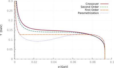
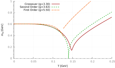
Figure 1: The phase diagram for the linear $\sigma$ model in mean-field approximation at $\mu_{\mathrm{B}}=0$, $\left\langle{\vec{\pi}}\right\rangle=0$. Left: the order parameter $\left\langle{\sigma}\right\rangle$ and the effective $\sigma$ mass $m_{\sigma}=\partial^{2}\Omega/\partial\sigma^{2}$.

To simulate non-equilibrium simulations we employ our recently developed semiclassical Monte-Carlo algorithm DSLAM (Dynamical Simulation of a Linear Sigma Model) Wesp:2014xpa to evaluate the dynamics of the $\sigma$ mean field on the one hand and the quarks as particles in a Boltzmann-transport approach on the other hand. The challenge here is that to achieve both thermal and chemical equilibrium besides the usual collision terms for $qq$ and $q\overline{q}$ elastic scattering one also has to take “chemical” processes like $q\overline{q}\leftrightarrow\sigma$ into account. Here, energy-momentum conservation as well as the principle of detailed balance have to be ensured to guarantee the correct equilibrium limit of the simulation.

Schematically our approach can be summarized in a stochastic mean-field and Boltzmann-Vlasov transport equation,

$$\Box\sigma+\lambda(\sigma^{2}-\nu^{2})\sigma-f_{\pi}m_{\pi}^{2}+g\left\langle{\overline{\psi}\psi}\right\rangle=I(\sigma\leftrightarrow\overline{q}q),$$ (5)

$$\begin{split}&\left[\partial_{t}+\frac{p}{E_{q}}\cdot\vec{\nabla}_{\vec{x}}-\vec{\nabla}_{\vec{x}}E_{\psi}(t,\vec{x},\vec{p})\cdot\vec{\nabla}_{\vec{p}})\right]f_{q}(t,\vec{x},\vec{p})\\ &\qquad=C(\psi\psi\rightarrow\psi\psi,\sigma\leftrightarrow\overline{q}q),\end{split}$$ (6)

where $I$ and $C$ denote collision terms contributing in a stochastic way to the time evolution of the mean field $\sigma$ and the quark phase-space distribution function $f$, respectively.

This scheme is numerically realized on a space-time grid, and the elastic binary collisions of the quarks are simulated with the usual stochastic Monte-Carlo method assuming a constant cross section of $\sigma_{\text{elastic}}=15\,\text{mb}$.

The decay process $\sigma\rightarrow\overline{q}q$ and the reverse recombination process $\overline{q}q\rightarrow\sigma$ are defined by the quantum field theory as processes involving the “particle picture”, leading to (perturbative) decay rates and cross sections in terms of the corresponding $S$-matrix elements. The corresponding “interaction processes” are considered as local, quasi-discrete, events in comparison to the involved macroscopic scales of the spatial and temporal changes of the mean field. Thus, within our mean-field approach to describe the mesons we need to define, how to transfer energy and momentum from and to the mean field corresponding to the stochastic and discrete decay and recombination processes.

For the recombination process, the initial state is already given in terms of the test quarks and anti-quarks, and the cross section is determined by the decay width of the $\sigma$ meson via the Breit-Wigner cross section

$$\sigma_{q\overline{q}\rightarrow\sigma}(s)=\frac{\Gamma^{2}}{(\sqrt{s}-m_{\sigma})^{2}+(\Gamma/2)^{2}}$$ (7)

with the decay width

$$\Gamma=\frac{g^{2}}{8\pi m_{\sigma}}\sqrt{1-\frac{4m_{q}^{2}}{m_{\sigma}^{2}}}.$$ (8)

Now energy-momentum conservation dictates the kinematics of the annihilation process, defining the energy and momentum, $\Delta E$ and $\Delta\boldsymbol{p}$, to be transferred to the classical $\sigma$ field. This is done by adding a Gaussian wave packet, taking into account the momentum in terms of a Lorentz boosted wave packet at rest. E.g., if the momentum is in $x$ direction one uses

$$\delta\phi(t,\boldsymbol{x})=A_{0}\exp\left[-\frac{\gamma^{2}(x-v_{x}t)^{2}+y^{2}+z^{2}}{2\sigma^{2}}\right]$$ (9)

with $v_{x}=p_{x}/E$ and $\gamma=(1-v_{x}^{2})^{-1/2}$. The width $\sigma$ is a free parameter of the model and characterizes an interaction volume; $A_{0}$ and $\boldsymbol{v}$ have to be determined by the change of the energy and momentum of the field, which is defined via the usual energy-momentum tensor,

$$E[\sigma] =\int_{V}\mathrm{d}^{3}\boldsymbol{x}\left[\frac{1}{2}\dot{\sigma}^{2}+\frac{1}{2}(\boldsymbol{\nabla}\sigma)^{2}+U(\sigma)\right],$$ (10)

$$\boldsymbol{P}[\sigma] =\int_{V}\mathrm{d}^{3}\boldsymbol{x}\dot{\sigma}\boldsymbol{\nabla}\sigma.$$ (11)

Then $A_{0}$ and $\boldsymbol{v}$ are determined such that

$$\Delta E=E[\sigma+\delta\sigma]-E[\sigma],\quad\Delta\boldsymbol{P}=\boldsymbol{P}[\sigma+\delta\sigma]-\boldsymbol{P}[\sigma],$$ (12)

where $\delta\sigma$ is defined by the Gaussian wave packet (9).

For the evaluation of the reverse decay process, $\sigma\rightarrow\overline{q}q$, we have to translate the mean-field description into a particle phase-space distribution function. To achieve this, we use the “coarse-graining” approach, i.e., we map the local energy-momentum distribution on the grid to local thermal-equilibrium distributions, i.e., we parameterize the phase-space distribution function of $\sigma$ particles by the Maxwell-Jüttner distribution,

$$f_{\sigma}(x,\boldsymbol{p})=\exp\left(-\frac{u\cdot p}{T}\right)=\exp\left[-\frac{\gamma}{T}(E-\boldsymbol{v}\cdot\boldsymbol{p})\right],$$ (13)

where

$$\boldsymbol{v}=\frac{\boldsymbol{P}[\sigma]}{E[\sigma]},\quad\gamma=\frac{1}{\sqrt{1-\boldsymbol{v}^{2}}},\quad u=\gamma\begin{pmatrix}1\\ \boldsymbol{v}\end{pmatrix}$$ (14)

denotes the collective flow-velocity field $\boldsymbol{v}$ and the four-vector flow field $u$ of the fluid cell $\Delta V$, respectively. The temperature, $T$, is fixed by demanding

$$\epsilon=\frac{E[\sigma]}{\Delta V}=\int_{\mathbb{R}^{3}}\frac{\mathrm{d}^{2}\boldsymbol{p}}{(2\pi)^{3}}\sqrt{m_{\sigma}^{2}+\boldsymbol{p}^{2}}f_{\sigma}(x,\boldsymbol{p}).$$ (15)

Hereby, the $\sigma$ mass and temperature $T$ are determined self-consistently with the $\sigma$ mass corresponding to the equilibrium value at this temperature.

Now the phase-space distribution function $f_{\sigma}$ is used in a Monte-Carlo step to determine a $\sigma$ meson which decays within the time step according to the decay rate ($\sigma$ width) (8). The corresponding energy and momentum of the decayed $\sigma$ meson is taken out of the $\sigma$ field by again subtracting the appropriate Gaussian wave packet (9) in the same way as explained above in connection with the quark-anti-quark annihilation process, and the quark and anti-quark with their respective momenta, also determined by the Monte-Carlo step, are added to the test-particle sample.

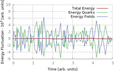
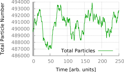
Figure 2: (Color online) Left: Energy fluctuations of the mean field and the quarks, $\Delta E=E(t)-\left\langle{E}\right\rangle$. Due to the $\sigma$ decay and quark-anti-quark annihilation processes energy is exchanged between the mean field and the particles, leading to thermal fluctuations $|\Delta E|/E\sim 10^{-2}$ for the field and $|\Delta E|/E\sim 10^{-3}$ for the quarks and anti-quarks. The total energy is conserved up to numerical fluctuations of $|\Delta E_{\text{tot}}/\left\langle{E}\right\rangle\lesssim 5\cdot 10^{-5}$. Right: Fluctuations of the total quark number due to $\sigma$-decay and $q\bar{q}$-annihilation processes.

2.2 Test calculations in equilibrium

To validate the above defined algorithm to simulate the kinetics of the linear $\sigma$ model in our particle-field approach, we have performed some numerical tests by simulating a microcanonical ensemble in a finite-size cubic box employing periodic boundary conditions. The number of test particles is $N_{\text{test}}=3\cdot 10^{6}$, the numerical time steps $\Delta t=2\cdot 10^{-3}\text{a.u.}$ (a.u.: arbitrary units), the spatial grid for the field is $N_{\sigma}=128^{3}$, corresponding to a total volume $V=(6\;\mathrm{fm})^{3}$. The total simulation time is $300\;\text{a.u.}$ corresponding to $150000$ time steps. The interaction volume of the Gaussian parameterization of the wave packets (9) is $32^{3}$ grid points, i.e., approximately $1.5\%$ of the system volume. As an initial condition we have chosen equilibrium conditions at a given temperature.

In Fig. 2 we show the fluctuations of the field and quark-anti-quark energy (left) and the total quark number (right) due to the $\sigma$-decay and $q\bar{q}$ annihilation processes, which show thermal fluctuations around the equilibrium mean values, while the total energy is conserved with a numerical accuracy of $|\Delta E_{\text{tot}}/\left\langle{E}\right\rangle\lesssim 5\cdot 10^{-5}$.

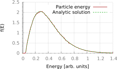
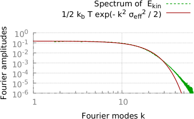
Figure 3: (Color online) Left: The energy distribution of the quarks and anti-quarks follow the expected relativistic Maxwell-Boltzmann distribution $f_{q}(E)\propto\exp(-E/T)$, demonstrating the numerical stability of the kinetic equations as well as the validity of the principle of detailed balance. Right: The spectrum of the kinetic energy density of the mean field, $\dot{\sigma}^{2}/2$. For low $k$ (long wavelengths) the distribution follows the expected equipartion theorem for a classical field, according to which each mode carries a mean energy of $1/2kT$, while at higher energies the finite interaction volume encoded in the finite width of the Gaussian wave packets leads to an effective cut-off $\sigma_{\text{eff}}^{2}=\sigma_{x}^{2}+\sigma_{y}^{2}+\sigma_{z}^{2}=3\sigma^{2}$.

As can be seen in Fig. 3, the energy distribution of the quarks and anti-quarks (left panel) follows the expected relativistic Maxwell-Boltzmann distribution

$$\frac{\mathrm{d}N}{\mathrm{d}E\mathrm{d}^{3}\boldsymbol{x}}=\frac{1}{2\pi^{2}}E\sqrt{E^{2}-m_{q}^{2}}\exp\left(-\frac{E}{T}\right)$$ (16)

with high numerical accuracy, which demonstrates again the good fulfillment of energy conservation as well as the principle of detailed balance for the elastic quark/anti-quark scattering and the “chemical” processes $q\overline{q}\leftrightarrow\sigma$. In the right panel we show the spectrum of the kinetic energy of the mean field, $\dot{\sigma}^{2}/2$. From classical field theory one expects a constant average energy of $k_{\text{B}}T$ for each mode, which is indeed the case for small wave number $k$, i.e., long wave lengths $\lambda=2\pi/k$. At lower wave lengths the finite interaction volume encoded in the finite width of the Gaussian wave packets (9) used to describe the energy-momentum transfer in the interaction between quarks/anti-quarks and $\sigma$ mesons from and to the mean field, leads to an effective cut-off of $1/\sigma_{\text{eff}}^{2}=\sigma_{x}^{2}+\sigma_{y}^{2}+\sigma_{z}^{2}=3\sigma^{2}$, i.e., the power spectrum is expected to follow Wesp:2014xpa

$$\frac{\mathrm{d}E_{\sigma}}{\mathrm{d}k}=\frac{1}{2}k_{\text{B}}T\exp\left(-k^{2}\sigma_{\text{eff}}^{2}/2\right).$$ (17)

The deviations from this result at very high modes can be explained by the non-linear potential in the mean-field equations of motion.

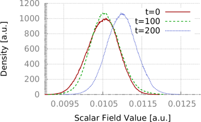
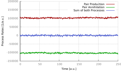
Figure 4: (Color online) Left: The distribution of the scalar field around its equilibrium value shows the expected Gaussian shape. The mean field can drift slowly with time due to the particle-field interactions. The quark-annihilation processes increase the local fluctuations, while particle production damps them by dissipating energy from the field. Right: Volume integrated rates for the pair-production and pair-annihilation processes, $\sigma\leftrightarrow\overline{q}q$, demonstrating the good fulfilment of the principle of detailed balance.

In Fig. 4 (left) we show the distribution of the scalar-field values around their mean as a function of time. Due to the quark-antiquark annihilation and $\sigma$-decay processes the mean-field value can drift slowly, while the fluctuations lead to the expected Gaussian distribution around this average. The local fluctuations of the field are increased by $q\overline{q}$ annihilation and damped by $\sigma$ decay. On the right-hand side the corresponding volume-integrated rates are plotted, demonstrating the good fulfillment of the principle of detailed balance within our simulation, which guarantees the right chemical equilibrium in the long-time limit.

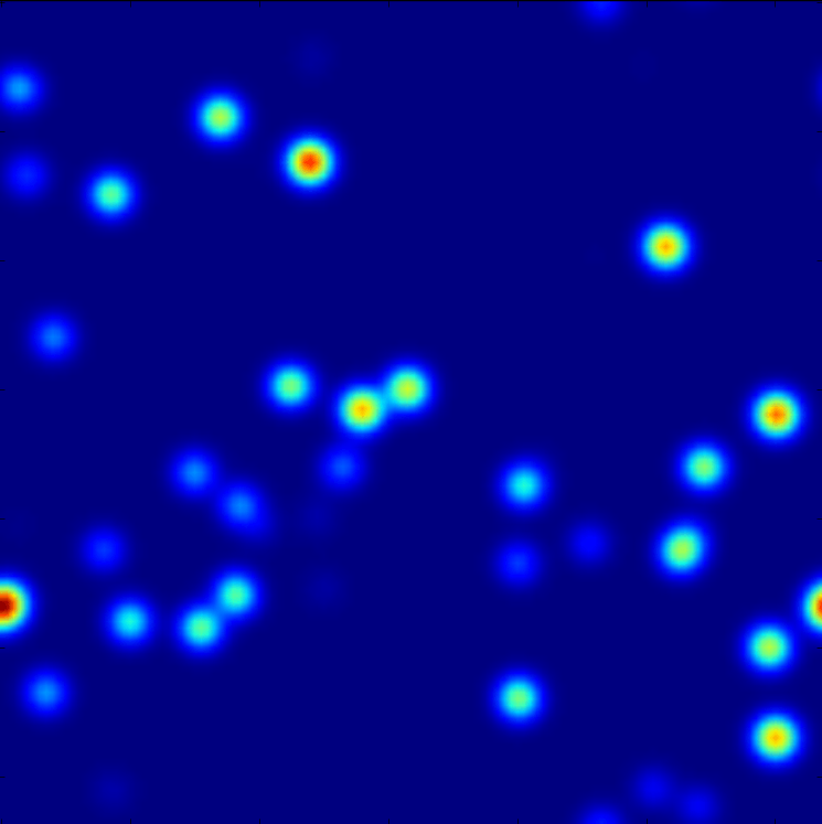
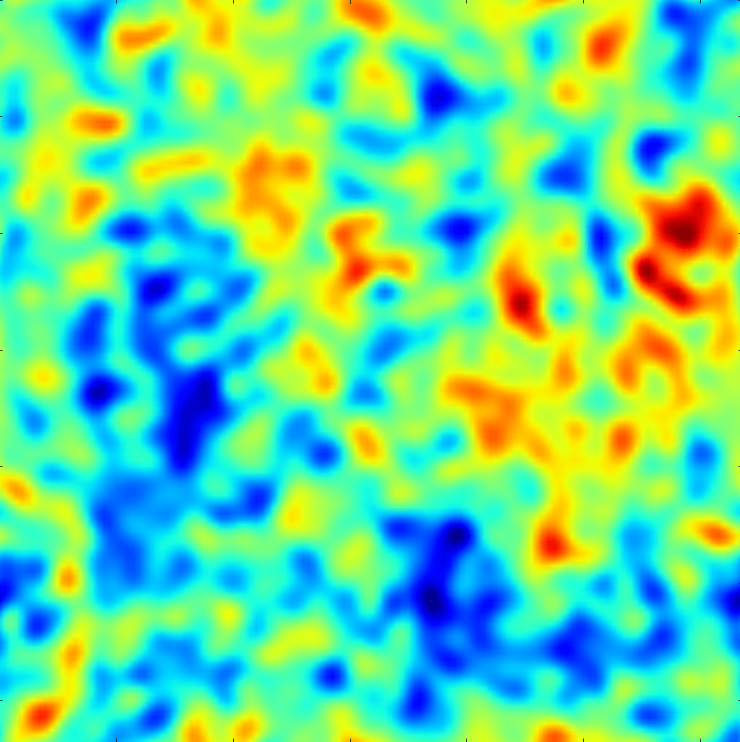
Figure 5: (Color online) Contour plot of the scalar field in an $x$-$y$-plane cut. The field is initialized with a uniform scalar field without excitations. Due to $q\overline{q}$ annihilation, field fluctuations build up, leading to single Gaussian excitations around the respective random interaction regions at early times (left). The right panel shows the field fluctuations after chemical equilibrium has been reached, leading to the expected thermal fluctuations of the field with height and strength scaling with temperature.

In Fig. 5 we demonstrate the chemical-equilibration process with a contour plot of the scalar field in an $x$-$y$-plane cut. Initially we have chosen a uniform field without any excitations. At early times (left panel) one can see the excitations of the field due to $q\overline{q}$ annihilation in terms of Gaussian blobs around the random interaction regions. At later times, when chemical equilibrium is reached (right panel), i.e., the particle-annihilation and creation rates become equal, we observe the expected thermal fluctuations. Their spatial width is determined by the interaction volume governed by the standard deviation, $\sigma$, parameterizing the interaction volume in the Gaussian wave packets (9). The height and strength of the fluctuations in the equilibrium limit is governed by the temperature $T$ of the system in accordance with the above discussed power spectrum (right panel of Fig. 3).

2.3 Thermal quench

As another test of the field-particle algorithm we initialize the kinetic equations in an off-equilibrium “thermal quench” situation in an isotropic periodic box. Initially the quarks are sampled at a temperature $T_{q}=140\;\mathrm{MeV}$ and the $\sigma$ field at its equilibrium value for $T_{\sigma}=180\;\mathrm{MeV}$. The coupling is set to $g=3.3$ corresponding to a cross-over chiral transition.The $q\overline{q}$-annihilation cross section is determined with the corresponding Breit-Wigner cross section as described above. Additionally a constant elastic $qq\rightarrow qq$-scattering cross section, $\sigma_{\text{elastic}}=15\;\mathrm{mb}$ is employed. We use a number of test particles $N_{\text{test}}=2\cdot 10^{6}$ and a time-step size of $\Delta t=0.002\;\mathrm{fm}/c$.

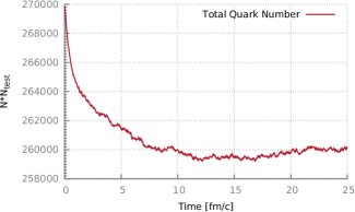
(a) Total number of quarks in the system.

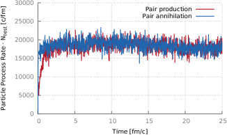
(b) Reaction rate for pair-production and pair-annihilation.

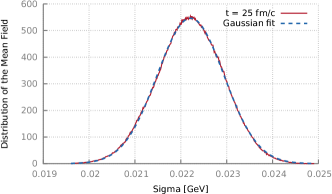
(c) Spatial distribution of the sigma mean field $\langle\sigma(\boldsymbol{x})\rangle$ after thermalization time $t=25\ \textrm{fm}/\textrm{c}$.

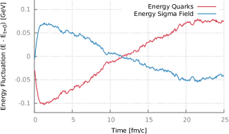
(d) Deviation from the initial energy for the quarks and the energy of the field, calculated with $E(t)-\langle E(t=0)\rangle$.

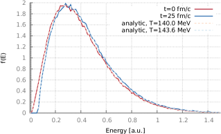
(e) Distribution of the quarks at the beginning of the system and after global thermalization.

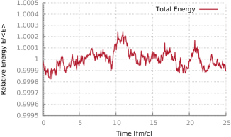
(f) Relative fluctuations of the system’s total energy $E(t)/\langle E(t=0)\rangle$.

Figure 6: (Color online) Results for a calculation with the quenched-scenario. Particles and fields can interact and their interaction rates converge after some time, leading the same global temperature of $T_{\text{eq}}\simeq 144\;\mathrm{MeV}$. The temperature of the quarks is given by the Boltzmann-distribution, the temperature of the field is given by the distribution of the field modes as expected from a power spectrum $S(k)=T/k^{2}$ as in a Langevin approach.

As shown in Fig. 6(a) the total quark number, i.e., the number of quark-antiquark pairs, drops rapidly in the beginning due to the annihilation and creation processes $q\overline{q}\leftrightarrow\sigma$, which (according to Fig. 6(b)) converge after about $10\;\mathrm{fm}/c$, fluctuating around the common mean-field value. Thermal equilibrium is roughly reached after about $20\;\mathrm{fm}/c$, leading to a common global temperature of about $T_{\text{eq}}\simeq 144\;\mathrm{MeV}$ as demonstrated by Figs. 6(c) and 6(e): at $t=25\;\mathrm{fm}/c$ the quark distribution is given by a Boltzmann distribution at this temperature, and the $\sigma$ field shows a Gaussian distribution around its equilibrium mean value. The temperature change of the quarks due to the transfer of initial potential field energy by only about $4\;\mathrm{MeV}$ is small, because the field’s initial potential energy is much smaller as compared to the energy of the quarks. As one can see in Figs. 6(d) and 6(f), energy between the quarks and the field is exchanged, while the total energy is conserved with high accuracy. As can be seen from Fig. 6(a) the particle number still rises slowly, and the system has not fully reached equilibrium. Also the mean-field value is not exactly at the equilibrium value shown in Fig. 1. The final approach to exact chemical equilibrium is very slow since the difference in the $\sigma$ potential is very small in this temperature range around the cross-over transition, resulting in a weak driving force. This underlines the importance of the “chemical” processes $q\overline{q}\leftrightarrow\sigma$ for a description of the global thermalization of the system to the expected global equilibrium as described by the phase diagram shown in Fig. 1.

In the next example we choose the same parameters as in the previous one but start with a lower Temperature of $T_{q}=80\;\mathrm{MeV}$ for the quarks. The $\sigma$ field has been initialized at the value $\left\langle{\sigma}\right\rangle\simeq 10\;\mathrm{MeV}$ in the chiral restored phase. Initially the quark number raises slightly due to $\sigma$-decay processes as shown in Figs. 7(a) and 7(b) while the mean field also increases moving towards the cross-over transition to the chiral broken phase. At some point of the evolution the $\sigma$ mass drops below the threshold for the decay to quark-anti-quark pairs, $m_{\sigma}<2m_{q}$, and the field becomes undamped and thus keeps oscillating for the rest of the time evolution (Fig. 7(e)). This non-equilibrium state stays in this oscillating state after about $10\;\mathrm{fm}/c$. The field shows again a Gaussian distribution around its average (Fig. 7(c)), and energy is exchanged with the quarks (Fig. 7(d)) via the Vlasov terms in Eqs. (5) and (LABEL:2.6). In Fig. 7(f) one sees that the spatial distribution of the $\sigma$ field shows the corresponding oscillations of the mean value and the stochastic fluctuations which persist from the time when the dissipative processes $\sigma\leftrightarrow q\overline{q}$ cease.

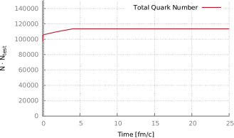
(a) Total number of quarks in the system.

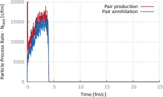
(b) Reaction rate for pair-production and pair-annihilation.

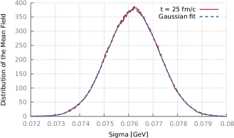
(c) Spatial distribution of the mean $\sigma$ field $\langle\sigma(\boldsymbol{x})\rangle$ in the stationary non-equilibrium state at $t=25\ \textrm{fm}/c$.

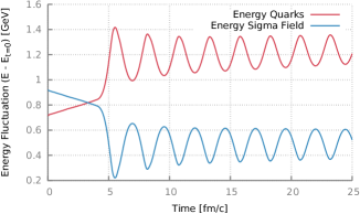
(d) Deviation from the initial energy for the quarks and the energy of the field, calculated with $E(t)-\langle E(t=0)\rangle$.

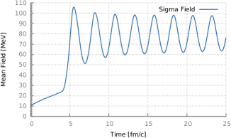
(e) Volume averaged value of the $\sigma$-mean field.

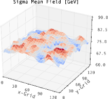
(f) Spatial distribution of the $\sigma$-field at $t=25\ \textrm{fm}/\textrm{c}$.

Figure 7: (Color online) Results for a calculation with the quenched-scenario from the initially hot phase to the cold and chiral broken phase. Fields and particles can interact above $T_{c}$ and the global shift of the $\sigma$-field is damped by particle production. At and below $T_{c}$ field and particles decouple because the $\sigma$-particle can not decay anymore. The system becomes undamped and falls in a coherent oscillation.

3 Simulations of an expanding fireball

To investigate a situation more close to the medium produced in heavy-ion collisions we initialize the system as a droplet with a Woods-Saxon like spherically symmetric temperature distribution

$$T(\boldsymbol{x})=T_{0}\left[1+\exp\left(\frac{|x|-R_{0}}{\alpha}\right)\right]^{-1}.$$ (18)

For this exploratory study we first work with a small system, corresponding to $R_{0}=0.45\;\mathrm{fm}$ and surface thickness $\alpha=0.1\;\mathrm{fm}$. The total system size has been chosen to $5\;\mathrm{fm}$. Also the boundary conditions have to be adapted from the so far used periodic boundary conditions to ones that allow for the expansion of the system. For the particles we choose a “distance cutoff” $r_{c}=2.75\;\mathrm{fm}$ from the center, where the particles are removed from the system.

The boundary conditions for the field is more complicated. Ideally one would choose absorbing boundary conditions (ABC), which perfectly absorb every wave traveling through the boundary and all its energy engquist1977absorbing . Unfortunately, such boundary conditions are very hard to implement and are computational expensive, especially in three dimensions and to have a good performance their formulation needs to be non-local in time Givoli2004319 . Still, they have been successfully applied for physical systems like the 3D Schrödinger equation PhysRevE.88.053308 .

To keep the computational cost reasonable, the boundary conditions are therefore kept periodic, but in the outer region of the box the $\sigma$-field is additionally damped by an effective friction $\propto\dot{\sigma}$ for any wave passing the cutoff radius $|\boldsymbol{x}|>r_{c}=2.75\;\mathrm{fm}$, leading to a strong damping of the waves. The total energy in this system is not conserved any more and any energy passing the boundary will be damped or removed from the system, preventing an interference with the rest of the system.

We have performed simulations for this expanding-fireball situation using both the model without and with the chemical processes $\sigma\leftrightarrow\overline{q}q$. The initial temperature was chosen $T_{\text{initial}}=175\,\mathrm{MeV}$, the number of test particles $N_{\text{test}}=10^{5}$, and a time step of $\Delta t=2\cdot 10^{-3}\;\mathrm{fm}/c$. Neglecting the chemical processes, the $\sigma$-field shows a rapid oscillation in the beginning of the expansion and loses energy mainly by radiating long-wavelength oscillations which propagate out of the system. Without any interaction processes the system stays nearly isotropic, only small spatial fluctuations of the quark-density lead to small deviations in the symmetry.

Additionally, for larger couplings the system can fall into a meta-stable state in which cold quarks are trapped in a potential well of the chiral field which has a long lifetime.

Here we concentrate on the results of simulations taking into account chemical processes $\sigma\leftrightarrow\bar{q}q$. These processes should lead to additional particle production whenever the $\sigma$-field shows strong fluctuations and particle annihilation in areas of high quark density, inducing additional fluctuations on the field. There are a couple of qualitative differences between the calculations with and without chemical processes. For all three different couplings ($g=3.3$, 3.63, and 5.5 corresponding to a cross-over, 2${}^{\text{nd}}$- and $1^{\text{st}}$-order chiral phase transition, respectively) the types of fluctuations are very different. The systems without chemical processes show strong global fluctuations, leading to shell-like structures with a fast oscillation of the chiral field at the origin of the matter droplet. The fluctuations are much less present in the calculations with chemical processes. The decay process $\sigma\rightarrow\bar{q}q$ damps such strong fluctuations by removing kinetic energy from the field. In contrast, the process $\bar{q}q\rightarrow\sigma$ creates strong local fluctuations on the field, increasing with a stronger coupling constant $g$. Additionally, all calculations without chemical processes stay nearly isotropic through their time evolution while the calculations with chemical processes show a breaking of this symmetry after a very short time. This symmetry is broken by strong and space-dependent fluctuations of the quark density and the field distribution and due to a collective drift of both particles and the field disturbance. Such a drift is surprising but is explained by the conservation of energy and momenta in the interactions between fields and particles. The $\sigma$-field can emit particles, generating a momentum-kick in the opposite direction of the particles, leading to a random-walk phenomena of the droplet. These outcomes are remarkable because no direct random processes are involved in the numerical simulation, which would create these fluctuations. All stochastic and fluctuating processes are the result of microscopic interaction kernels and cross-sections which are sampled via Monte-Carlo methods.

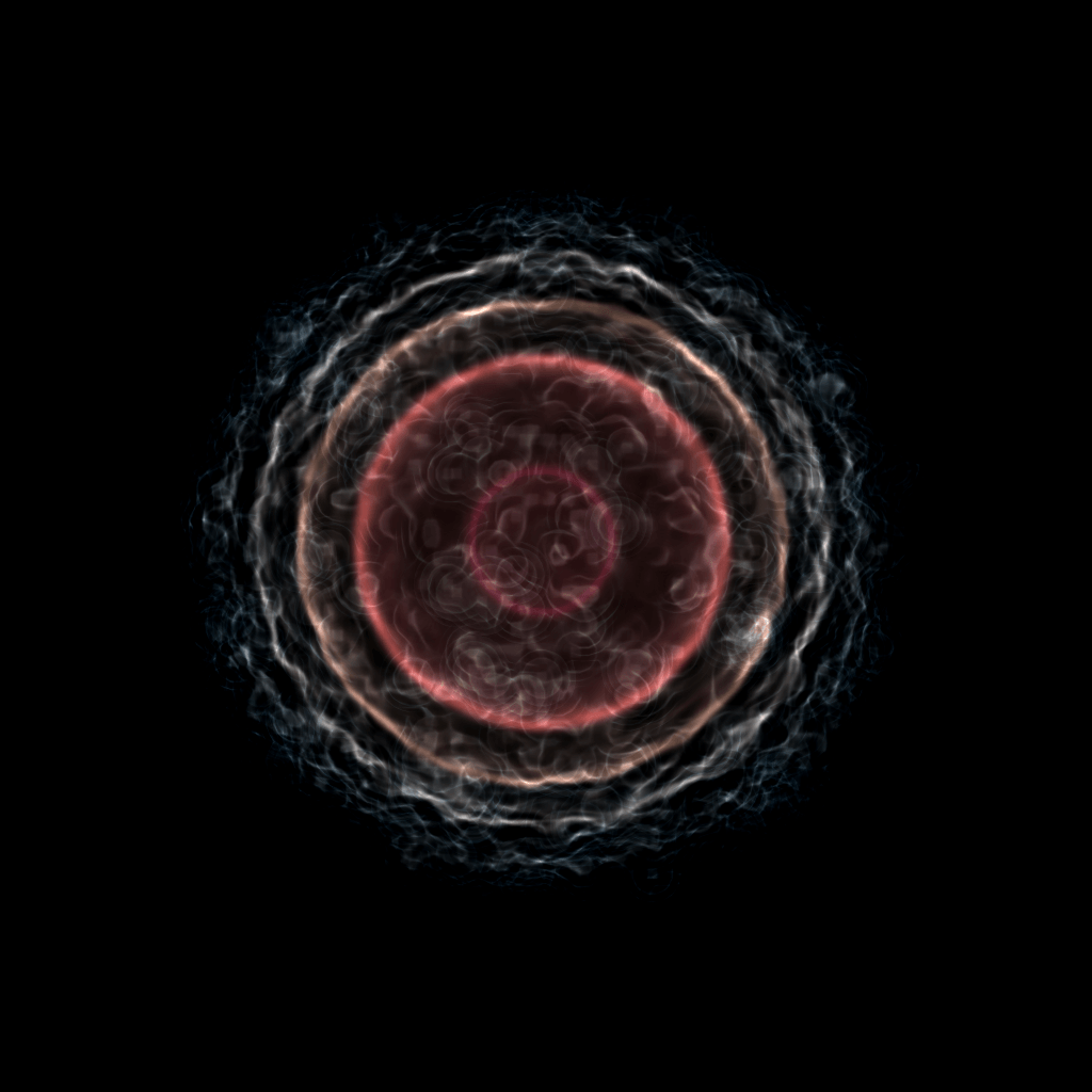
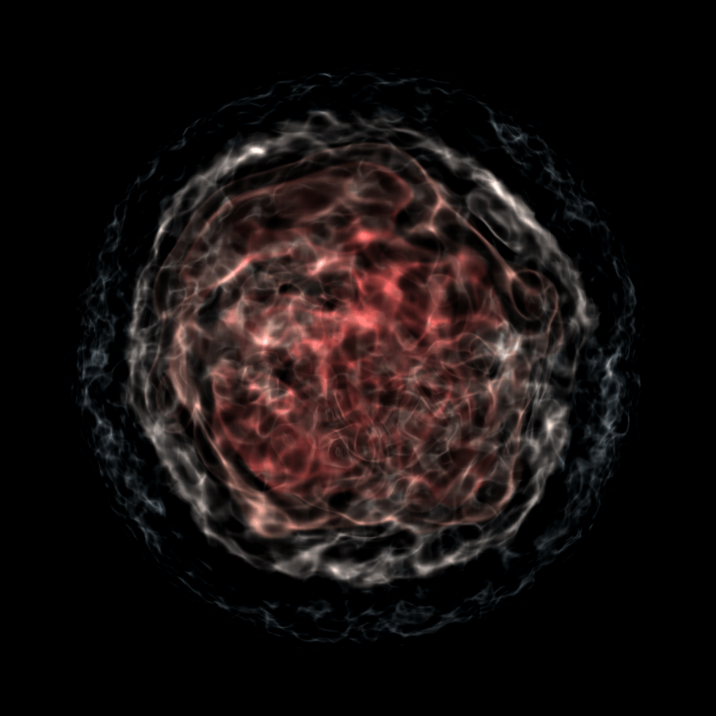
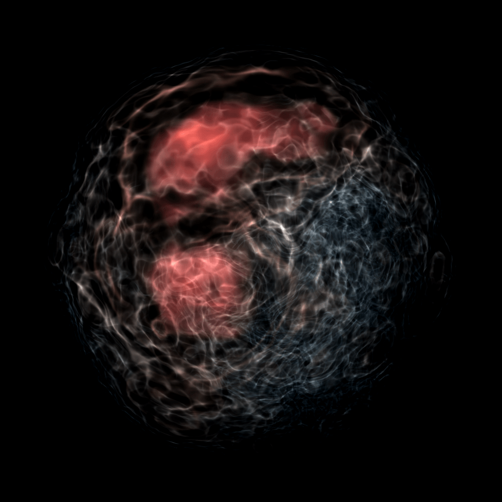
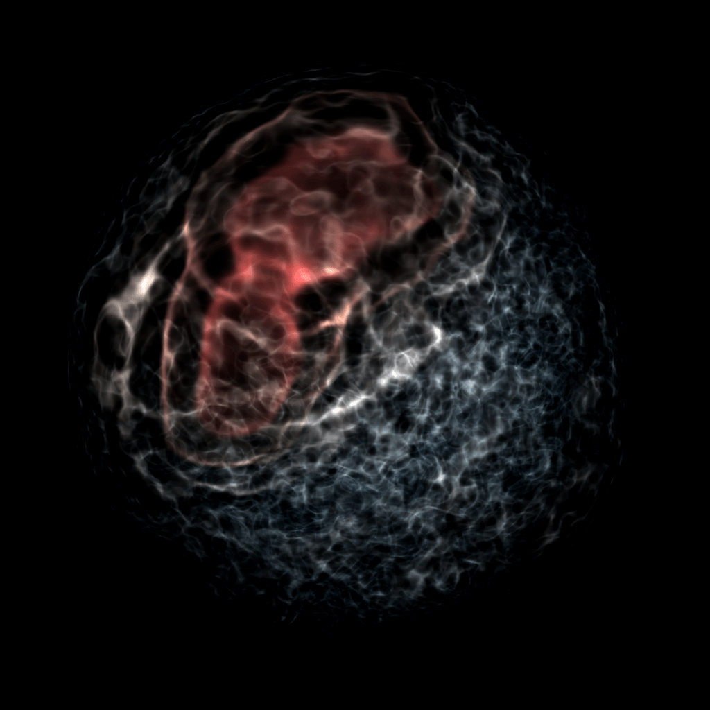
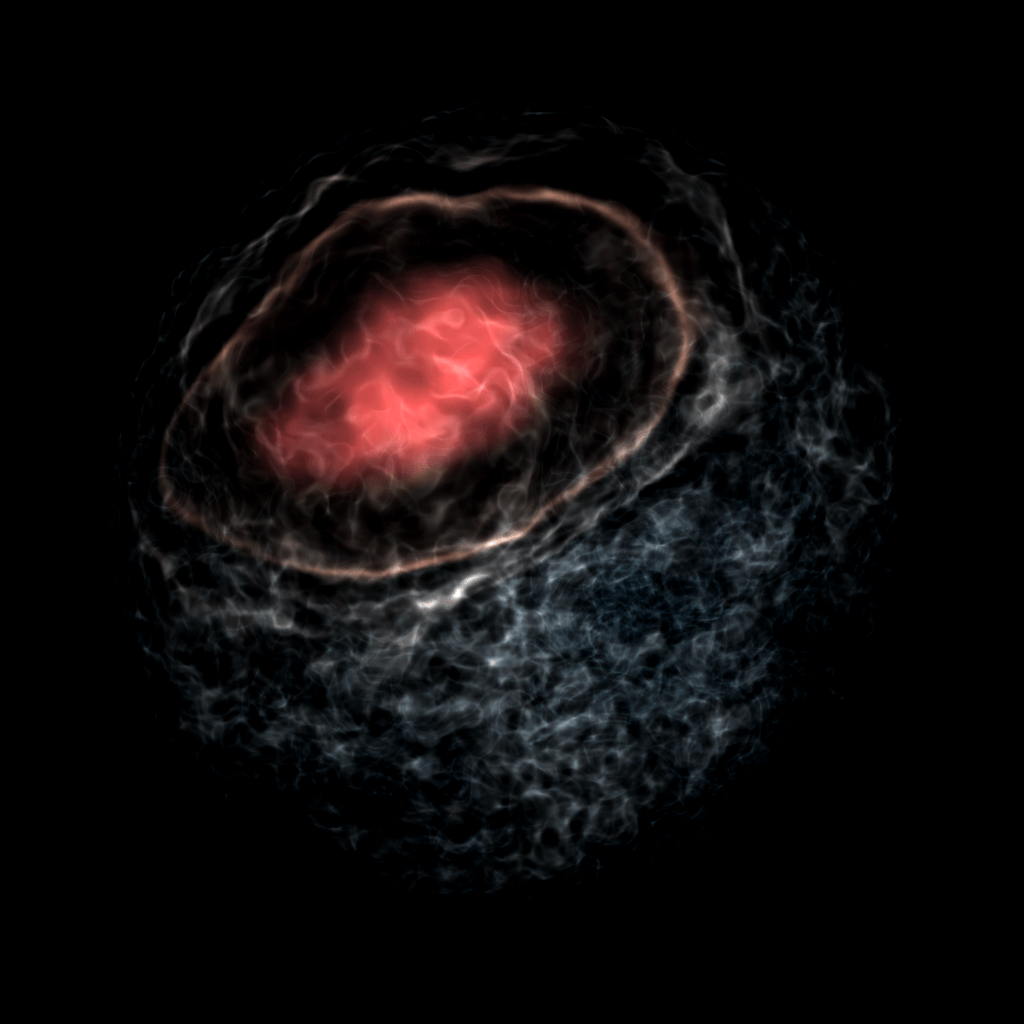
Figure 8: Volumetric 3D rendering of the quark density for the hot matter droplet scenario with a coupling of $g=5.5$, a first-order transition and chemical processes. The time progresses for $1\;\mathrm{fm}/\text{c}$ for every image. Regions with high particle densities are colored red, the scale is constant over all images. Visualization was created using the yt-toolkit Turk2010 .

By comparing the calculations with chemical processes with different couplings $g$, qualitative differences are visible, as well. The fluctuations in the field and particle density increase for stronger couplings. For a coupling of $g=5.5$ the quark density forms small regions with higher densities, which merge with time. These observations are consistent with calculations of the linear $\sigma$-model with a hydrodynamic background Nahrgang:2011mg ; Nahrgang:2011mv ; Herold:2013bi , in which the authors find the strongest fluctuations for a medium with a first-order phase transition. Classical theories of phase transitions in thermal equilibrium predict the strongest fluctuations at and near the phase transition for second-order transitions. Calculations presented here show the strongest fluctuations for the highest coupling associated with the first-order phase transition. At first, this scenario can not be directly compared to a phase transition. A phase transition is a phenomenon described by equilibrium physics for very large systems which evolve in the adiabatic limit on large time scales. In off-equilibrium situations fluctuations need time to build up via interactions within the bulk medium. Most important, the correlation length is often largely enhanced at the phase transition, which is no problem for systems which are much larger than this correlation length. The scenario of the hot-matter droplet is quite the opposite. The system size is in the order of the interaction length and therefore its correlation length. The quark matter expands rapidly and its dynamics creates distributions which strongly deviate from equilibrium, and the total lifetime of the system is at most in the order of the equilibration timescale. Additionally, a rapid expansion leads to a highly anisotropic system with gradients and parts of the system separate to regions with very different densities and temperatures. All these circumstances do not allow a consistent description of the system in terms of an equilibrium phase transition, especially not if the quarks are described by particles with non-equilibrium distributions and not by a fast equilibrating medium. Any deviation from equilibrium descriptions have a strong impact on the thermal properties of the medium.

Considering the system dynamics in terms of its transport properties would be a more adequate approach to the characteristics of its behavior. The strong fluctuations only occur if the chemical processes $\sigma\leftrightarrow\bar{q}q$ are present, their microscopic interaction kernels are derived from a Breit-Wigner cross-section. Larger couplings lead to a higher interaction rate between fields and particles (in our model $\sigma_{\sigma\leftrightarrow\overline{q}{q}}\propto g^{2}$). This already implies that the largest fluctuations build up for the calculations with the coupling $g=5.5$ and quite similar fluctuations for $g=3.3$ and $g=3.63$, even though these different couplings would show very different kind of phase transitions in an equilibrated system.

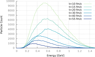
Figure 9: (Color online) Left: Total quark number in the matter-droplet scenario. Solid lines show the simulations with chemical processes, the dashed lines the simulations without the $\sigma\leftrightarrow\bar{q}q$ process. In the scenario without chemical processes the droplet radiates most of the quarks in shell-like structures, as reflected in the quark-number plateaus which drop suddenly. Due to condensation processes the system can form meta-stable states, in which cold quarks are trapped in a chiral-potential well, which can be observed in the stable, non-zero quark number for $g=5.5$ over long times. The behavior is completely different for the calculations with chemical processes, in which the systems lose quarks in a steady and continuous process, the formation of quark-number plateaus is washed out. Right: Energy distribution functions of the quarks in the simulation for the matter-droplet scenario with $g=5.5$ and chemical processes. After $10\;\mathrm{fm}/c$ most of the initial particles have left the system, and the remaining particles have formed a drop of cold quarks, which are trapped in a chiral-potential well. One can see a non-thermal distribution function in the beginning, which slowly thermalizes due to elastic interactions. However, mainly high-energy quarks can leave the potential well, leading to both a slow evaporation of the drop and to an effective cooling of the remaining particles.

Furthermore, two other aspects play an important role in the comparison of the different calculations. The coupling has a direct impact on the mass of the quarks. A higher coupling leads to a larger quark mass in the chiral broken phase. This implies both a larger particle number at the same temperature for a higher coupling and a larger potential energy for the chiral fields. The second aspect has its origin in the phase diagram. Higher couplings lead to a lower $T_{c}$ in the linear $\sigma$-model, which strongly changes the dynamics of the chemical interactions as they are only possible above the mass threshold, meaning above $T_{c}$. For lower $T_{c}$, in comparison to other couplings, the quarks and the fields have more time to stay in the chiral restored phase, more time to interact with each other and therefore more time to build up fluctuations via these interactions. This already implies stronger fluctuations, regardless of the type of phase transition, which would be given by the corresponding coupling. A fair comparison between the scenarios is not given by comparing the system at different temperatures. Better approaches could be a comparison with same energies or same particle number.

In the calculations neglecting chemical processes the formation of meta-stable drops of quarks could be observed, especially at the high coupling, $g=5.5$. This behavior can be seen in the simulations including chemical reactions, too. For $g=5.5$ with chemical reactions the system even shows something like bubble formation. Figure 8 shows a volumetric 3D rendering of the quark density which projects the full three dimensional density and visualizes how small areas of high quark-density start to merge into larger areas, having some similarity to the condensation of water drops in steam. The mechanism of this condensation is that it is the energetically favorable configuration for the $\sigma$-field. Interestingly, the condensation progresses and the $\sigma$-field looses energy by radiating wave excitations. The process seems to stop after $10\;\mathrm{fm}/\text{c}$ by forming a quasi-stable drop. The left panel in Figure 9 shows the total quark number of the system, showing a steady decrease of quarks in the system, indicating a kind of particle evaporation from the drop. This evaporation seems to be quite slow and calculations have shown a lifetime of up to $50\;\mathrm{fm}/\text{c}$ before the drop bursts. The right panel Figure 9 displays the evolution of the quark-distribution function with time after a condensation drop has been formed. The figure shows a decrease of the quark number with time, and mainly particles with high energies leave the system. This is reasonable because particles with high energy can escape the potential well, leading to a collective cooling of the remaining medium.

All calculations discussed so far are done for systems with a fireball which has an initial diameter of roughly $d\approx 1\;\mathrm{fm}$. In comparison to a heavy-ion collision such a system is very small. Both lead and gold nuclei have a diameter of around $d_{\text{Au}}\approx 14\;\mathrm{fm}$, resulting in a volume two orders of magnitude larger than in this scenario. Therefore quantified predictions for a heavy-ion collision can not be derived from these calculations. Both the number of involved quarks and the energy density in the system could lead to different phenomena. Additionally, a much larger spatial and time scale may change the behavior at the phase transition because the system has potentially more time to evolve and form structures in the particle densities.

Now we simulate the model with a larger system volume of $V=(36\;\mathrm{fm})^{3}$ with an initial size of the matter droplet of $d\simeq 14\;\mathrm{fm}$, roughly resembling a central Au-Au collision. The initial temperature was again chosen to be $T=175\;\mathrm{MeV}$, as well as the couplings $g=3.3$, $g=3.63$, and $g=5.5$ to investigate the cases of cross-over, 2${}^{\text{nd}}$, and $1^{\text{st}}$ order phase transitions. The grid size is increased to $N_{\text{grid}}=192^{3}$, and the time step is reduced to $\Delta t=10^{-3}\;\mathrm{fm}/c$. Also the interaction volume has been slightly increased to $V_{\text{interaction}}=(0.4\;\mathrm{fm})^{3}$. The total number of particles was $\sim 5\cdot 10^{6}$ with a test-particle multiplicator of $200$.

Figure 10 and 11 show the result for a calculation with a large expanding matter droplet. Both figures compare the same calculations with and without chemical interactions and different couplings, $g=3.3$ with a cross-over transition in Figure 10 and $g=5.5$ in Figure 11.

The calculations without chemical interactions do not change very much in comparison to the smaller systems. The overall symmetry of the system stays effectively intact, and known structures like the shell-structures Abada:1994mf ; Greiner:1996md and cold quark droplets are still present.

The qualitative picture changes somewhat for calculations with chemical interactions, especially for larger couplings like $g=5.5$. After a short expansion phase the matter droplet starts to form strong and non-isotropic structures in the quark density due to the annihilation and creation process. In Figure 10 first structures are already present at $t\approx 1\,\text{fm}/c$. These structures blur while the matter expands.

In Figure 11 these structures are much stronger and much finer. The reason is the strong coupling between the field and particles, leading to fast annihilation and strong damping of the field by $\sigma$-decay. While expanding, the fluctuations on the $\sigma$-field become stronger. Around $t=5\,\text{fm}/c$ the annihilation-rate of the quarks is negligible because of the low particle density due to expansion. The $\sigma$-decay becomes the dominating effect, leading to a strong damping of the field and to a quasi-freeze out of the field leading to some kind of local bubble-formation. The resulting field distribution stays stable for several $10\;\mathrm{fm}/c$ local bubbles converge slowly to a big drop. This final drop contains the already known cold quarks which were not able to escape the kinetic potential.

In the calculations for larger systems a qualitative difference between the couplings can be seen in the time evolution. While calculations for $g=3.3$ and $g=3.63$ behave similar, calculations for $g=5.5$ show a very different behavior: the quark matter forms bubbles and freezes out in a relative long-living structure.

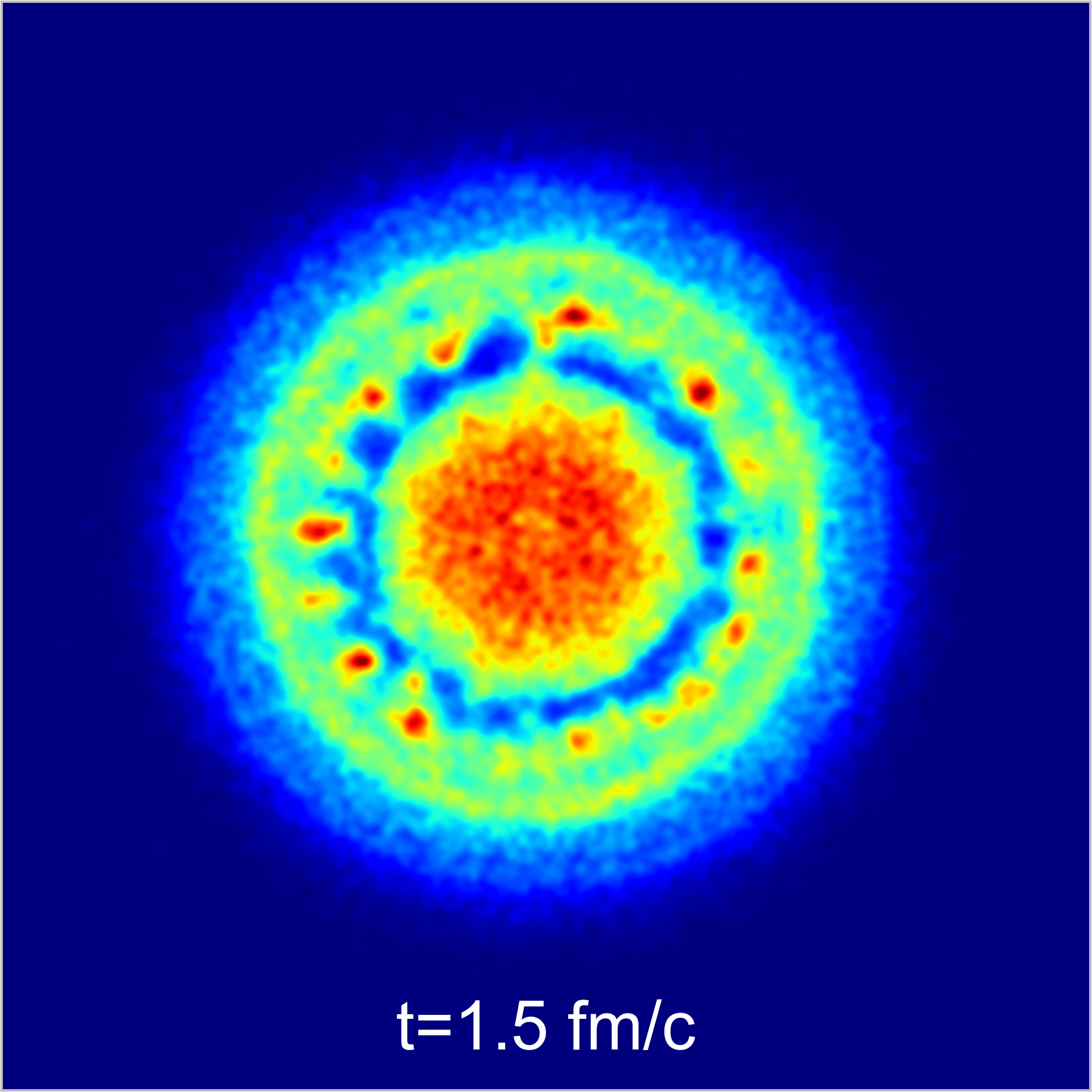
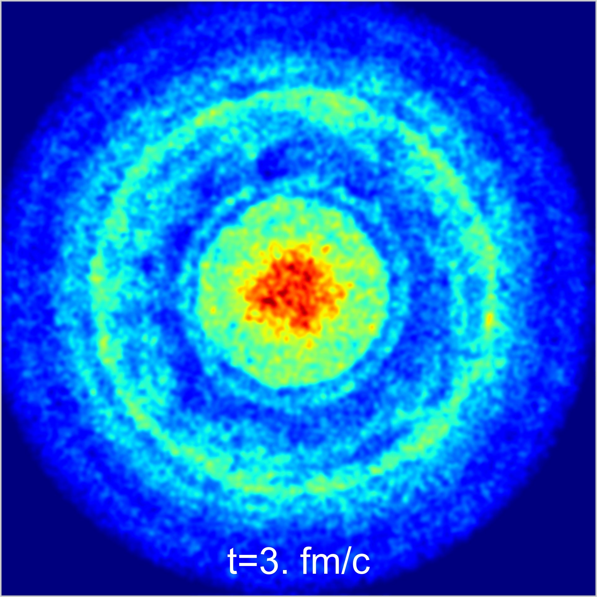
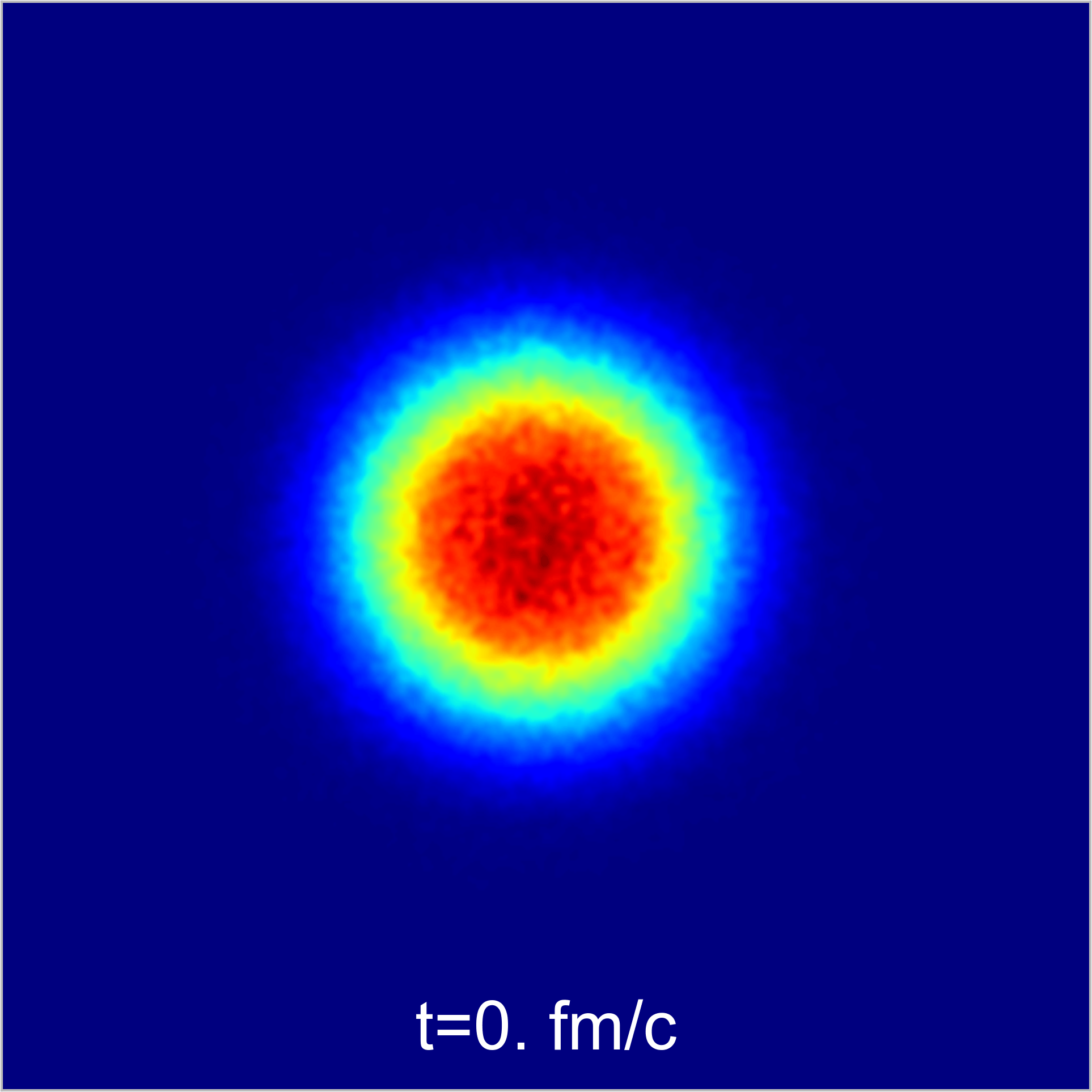
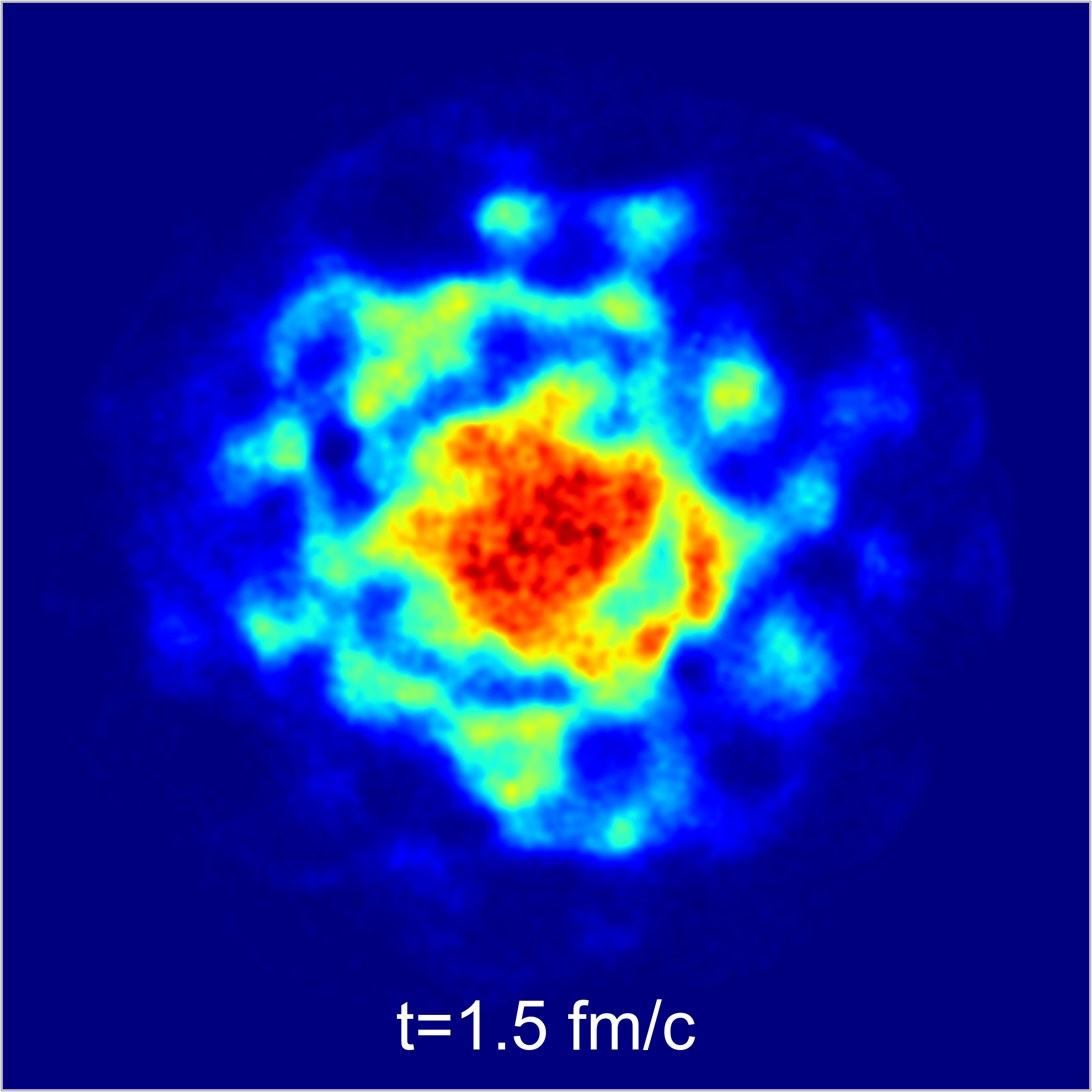
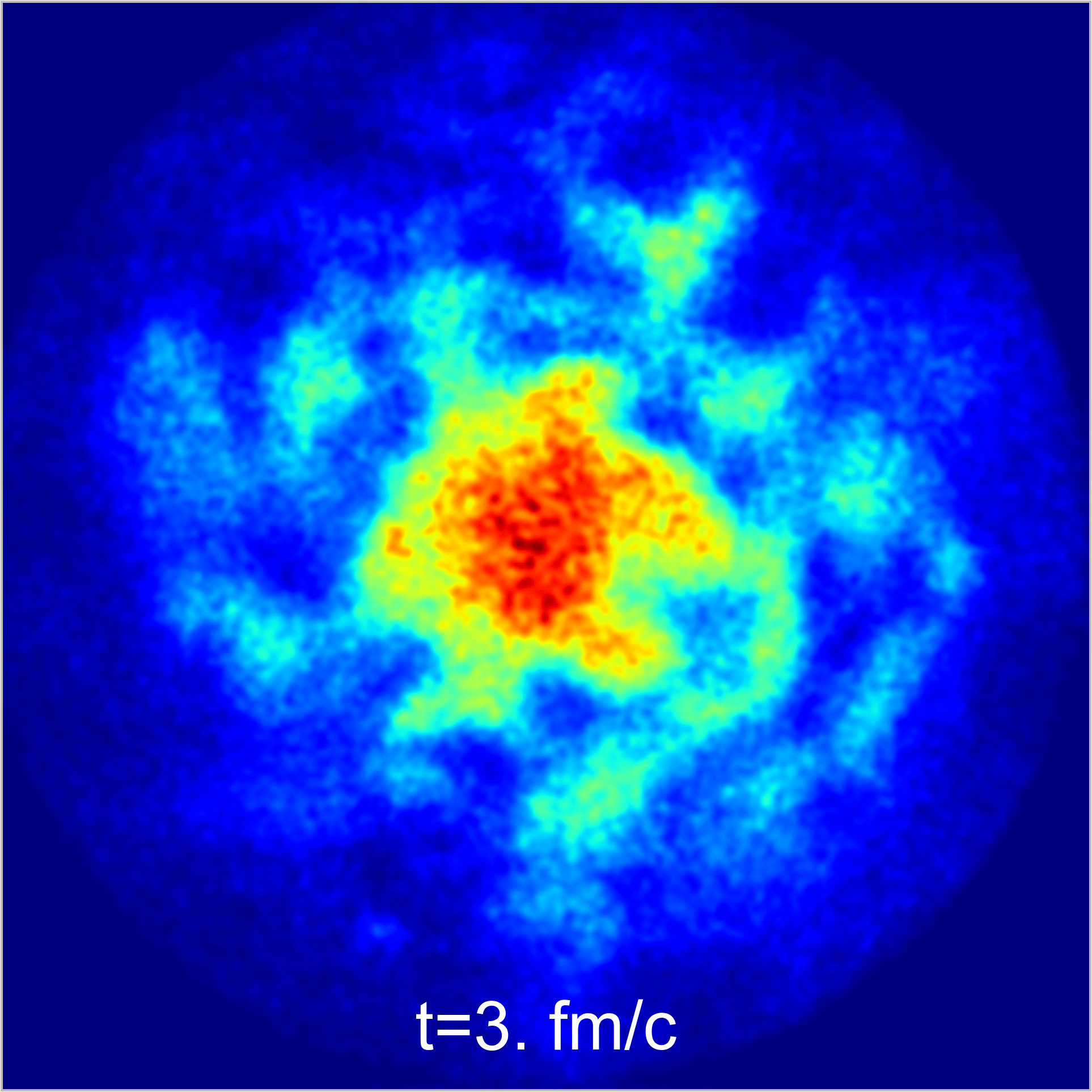
Figure 10: Evolution of the quark density for a large hot matter-droplet scenario with $g=3.3$. The initial size of the droplet has an diameter of around $d\approx 14\;\mathrm{fm}$ which corresponds to the size of a gold nuclei, the total size of the system is $V=(36\;\mathrm{fm})^{3}$. Left: Simulation without chemical interactions Right: simulation with chemical interactions. Chemical interactions lead to the formation of anisotropic structures, but the overall expansion of the system is not strongly altered.

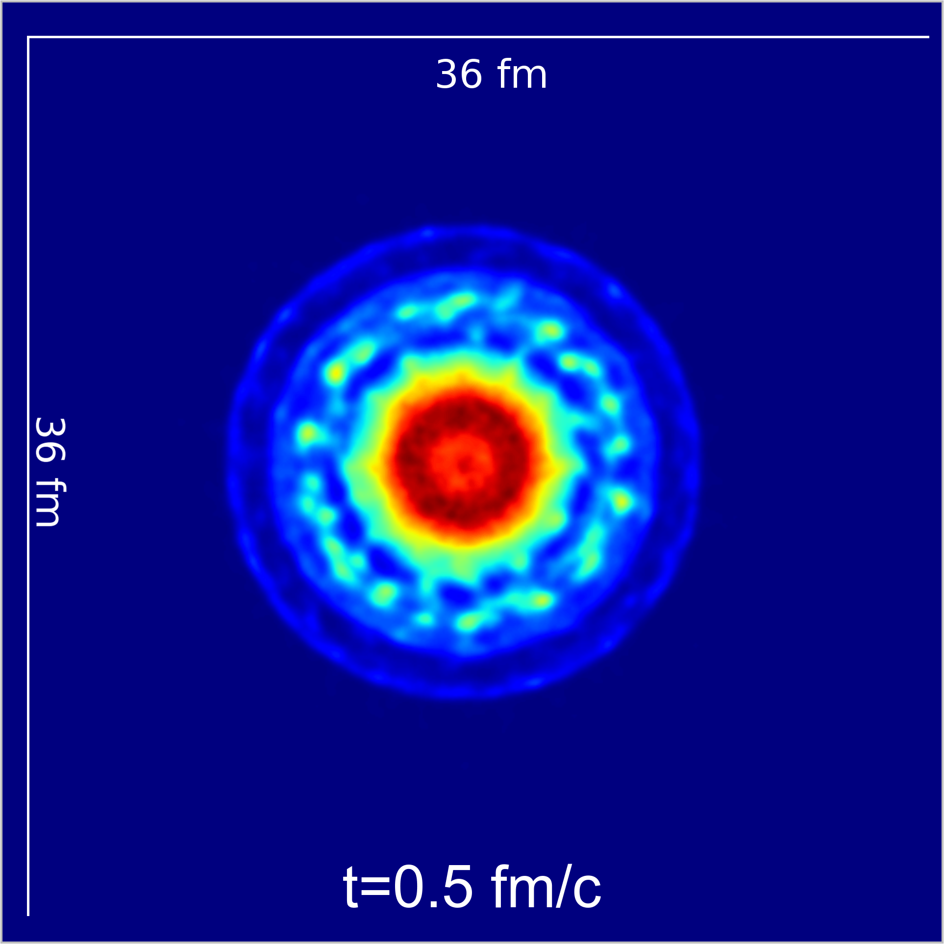
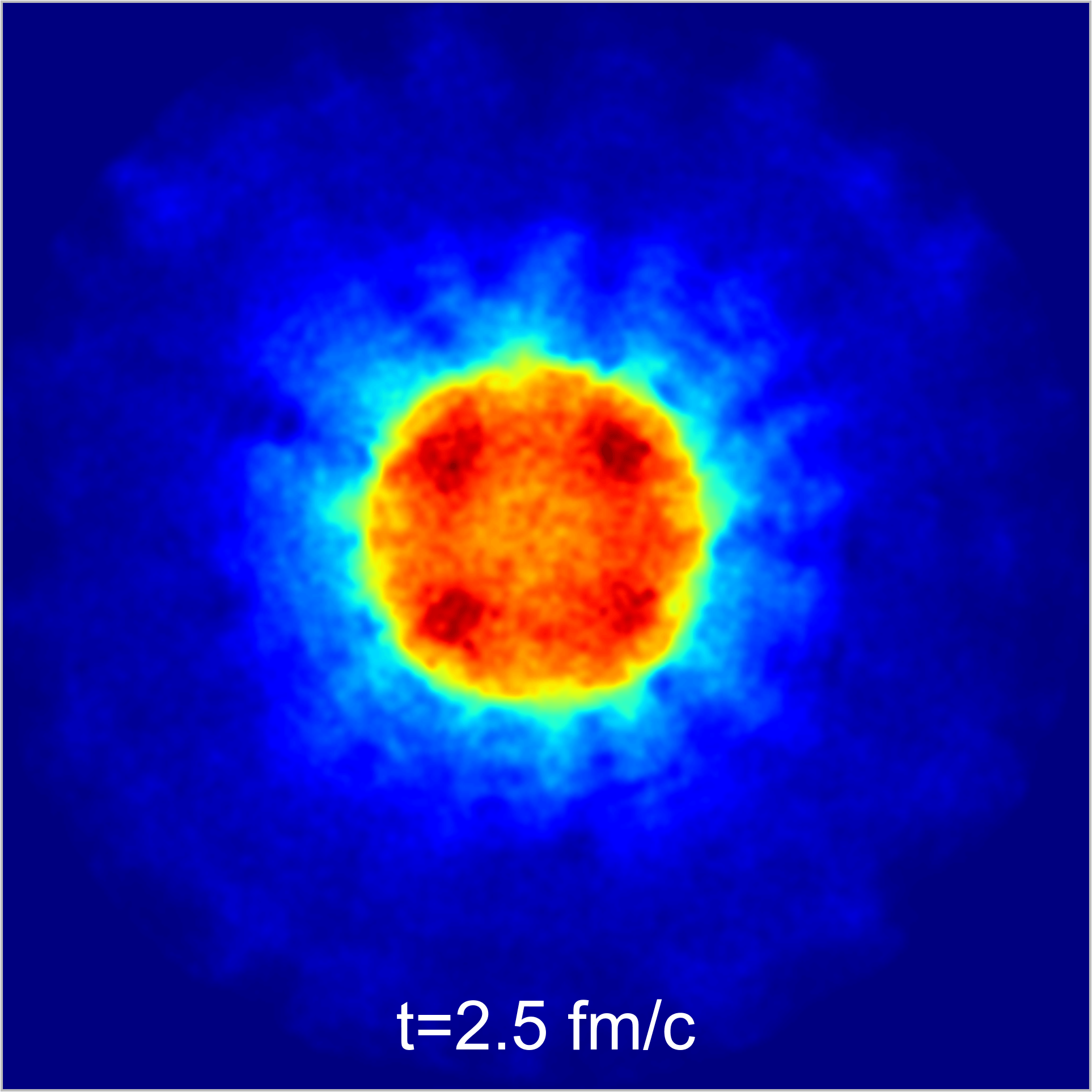
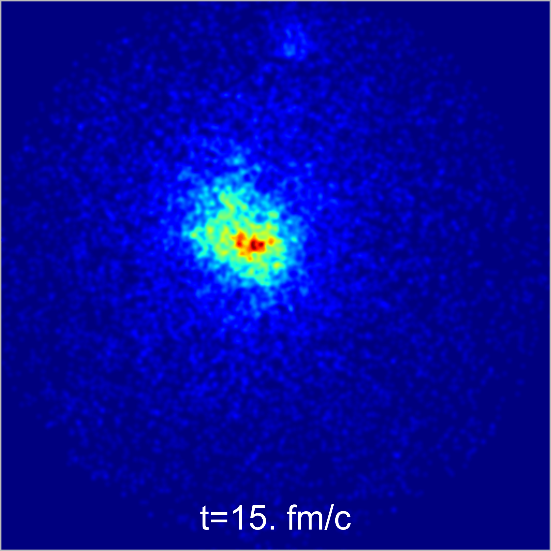
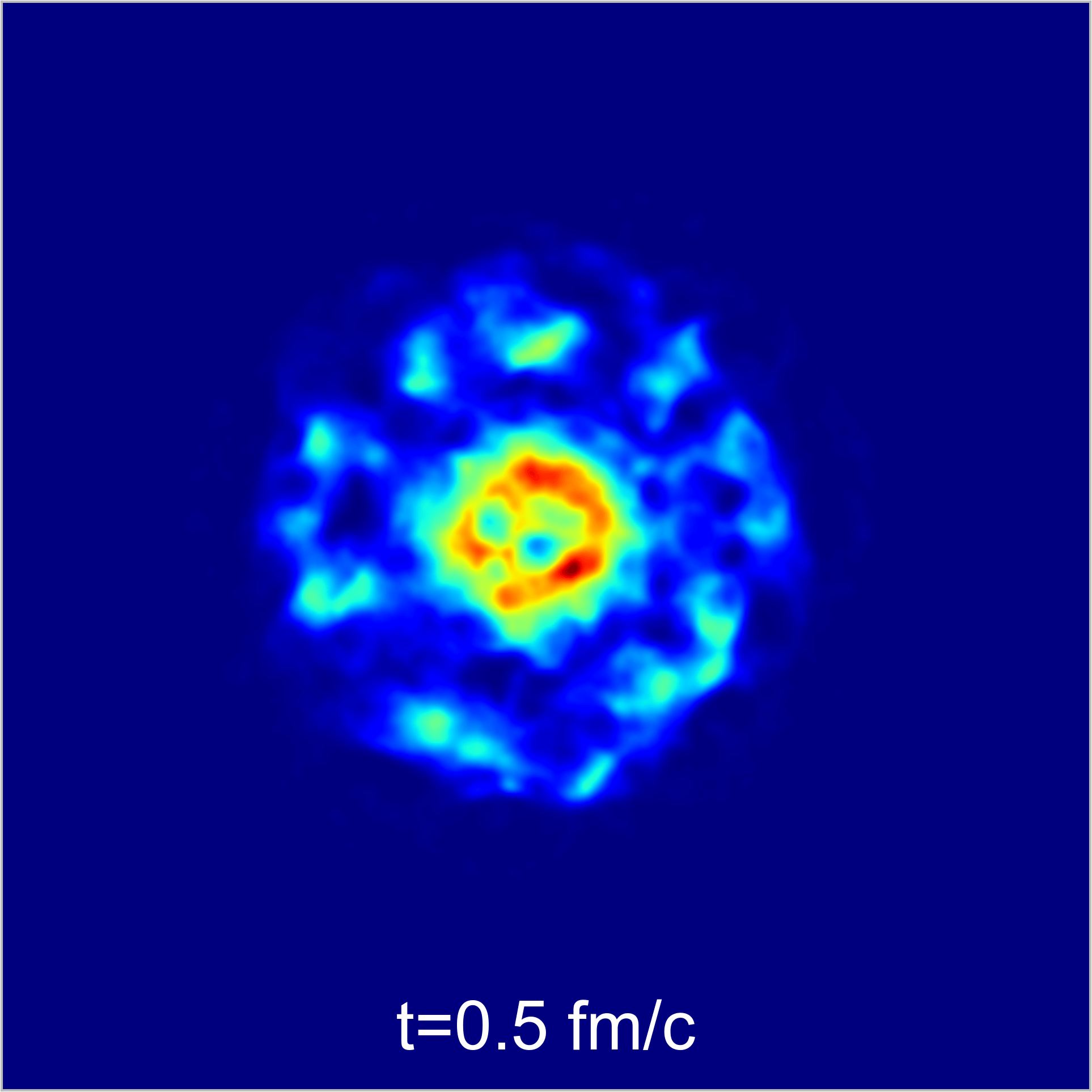
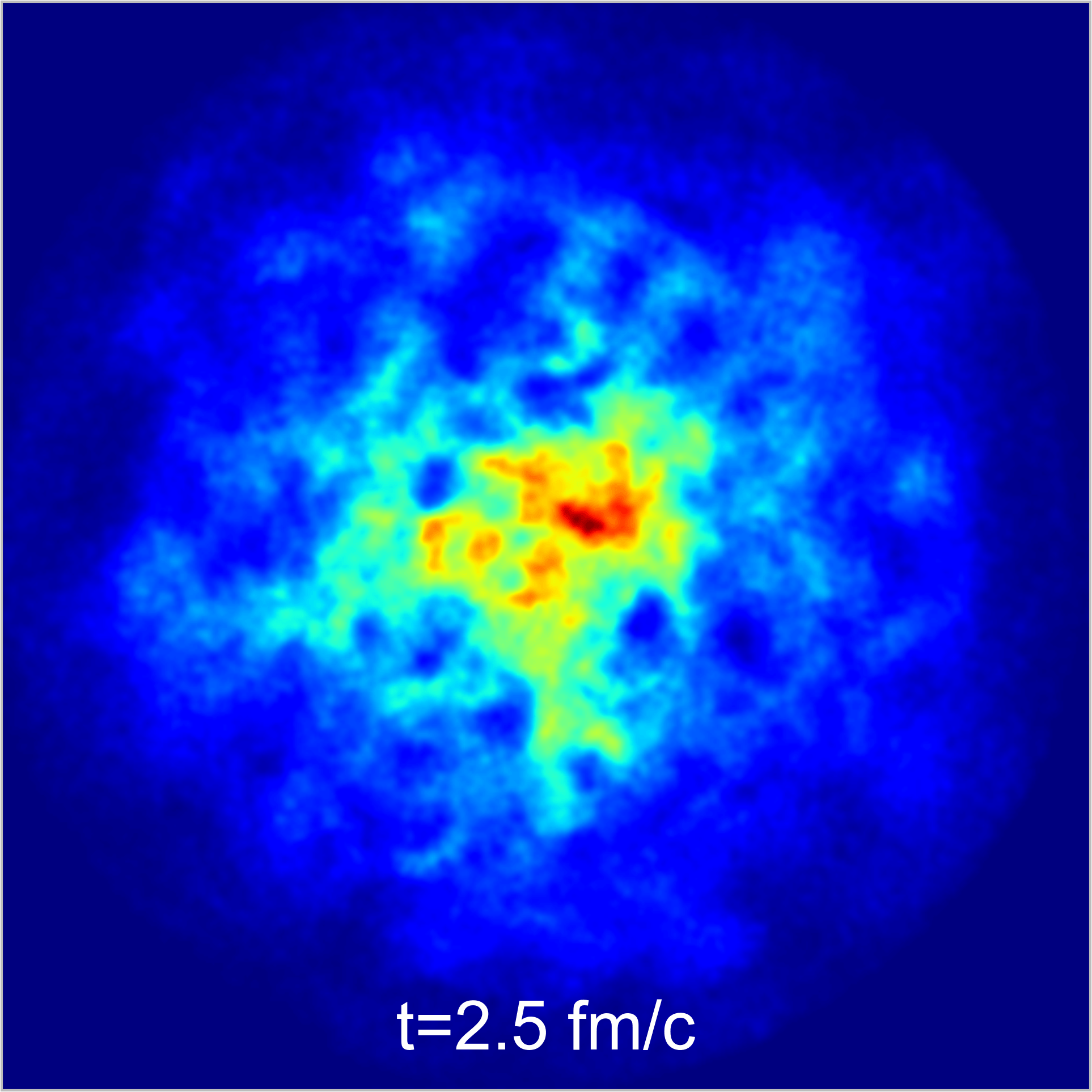
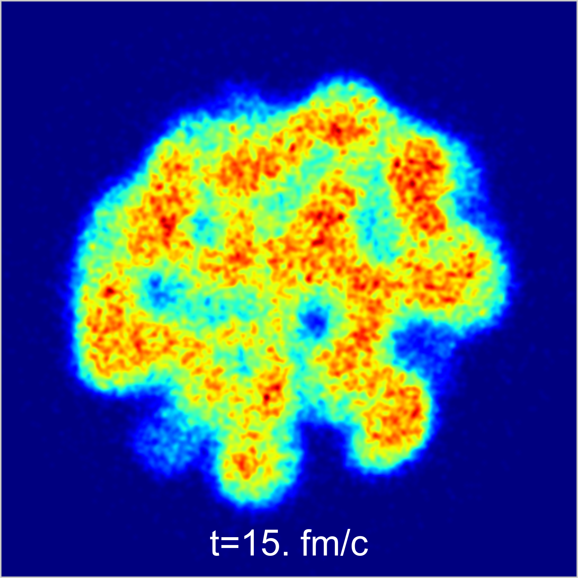
Figure 11: Quark density for a large hot matter-droplet scenario with $g=5.5$. The initial size of the droplet has a diameter of about $d\approx 14\;\mathrm{fm}$ which corresponds to the size of a gold nucleus, the total size of the system is $V=(36\;\mathrm{fm})^{3}$. Left: Simulation without chemical interactions Right: simulation with chemical interactions. Chemical interactions lead to a generation of strong and detailed structures. After $5\;\mathrm{fm}/c$ the expansion of the system is stopped by the strong damping of the field, leading to the formation of local bubbles.

The calculations in this section have shown the very interesting complexity of such a simple initial condition like an expanding matter droplet. The chemical reactions between particles have a very strong impact on the system behavior and dramatically change both fluctuations and medium propagation within the expansion. However, characteristic signatures which would allow an event-by-event discrimination between the different coupling strengths (implying different phase transitions in equilibrium) in this scenario has not been found, at least not for calculations with the cross-over coupling $g=3.3$ and the second-order transition coupling $g=3.63$. As a first attempt to quantify the quark-number fluctuations in Fig. 12 we plot the angular momentum distribution of quarks leaving the fireball volume for the case of $g=3.3$. The qualitative features of the distribution do not significantly vary with the coupling strength. Only for the first-order value $g=5.5$ show significantly larger magnitude of the fluctuations, as quantified by the power spectra of the angular correlation function.

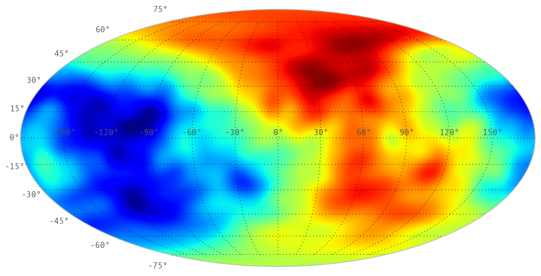
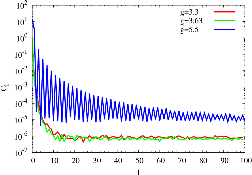
Figure 12: (Color online) Angular distribution (left panel) of quarks leaving the fireball for the coupling $g=3.3$ and the power spectrum of the angular correlation functions (right panel).

To quantify the angular distributions further, we evaluate the angular power spectrum, via

$$C_{lm}=\int_{\Omega}\mathrm{d}\Omega f(\vartheta,\varphi)\text{Y}_{lm}(\vartheta,\varphi)$$ (19)

with the usual normalized spherical harmonics $\text{Y}_{lm}(\vartheta,\varphi)$ and

$$f(\vartheta,\varphi)=\int_{0}^{\infty}\mathrm{d}p\frac{\mathrm{d}}{\mathrm{d}^{2}p}N_{\text{quark}}(p,\vartheta,\varphi).$$ (20)

The normalized power spectrum is then defined by

$$C_{l}=\frac{1}{2l+1}\sum_{m=-l}^{l}|C_{lm}|^{2}.$$ (21)

4 Conclusions and outlook

In this paper we have used a novel numerical algorithm to simulate the off-equilibrium dynamics of a quark-meson linear-$\sigma$ model (DSLAM) inspired by “wave-particle duality” of “old quantum mechanics”, guaranteeing accurate energy-momentum conservation and the principle of detailed balance by treating the quarks and anti-quarks, coupled to a $\sigma$ mean-field with the test-particle Monte-Carlo approach to evaluate the two-body elastic-collision terms and a combined method using wave-particle duality and coarse graining to evaluate chemical processes of quark-antiquark pair annihilation and $\sigma$-meson decay, $q\overline{q}\leftrightarrow\sigma$. On top also the mean-field equation for the $\sigma$ field has been solved consistently.

The algorithm has been validated in “box calculations” by checking the energy-momentum conservation, the stability of the expected equilibrium solutions for the mean field and quark-antiquark phase-space distribution functions, and the approach to the correct thermal and chemical equilibrium in the long-time limit starting with simple off-equilibrium initial conditions (“thermal quench”), demonstrating excellent fulfillment of energy-momentum conservation and of the principle of detailed balance. The implementation of the chemical processes $q\overline{q}\leftrightarrow\sigma$ are found to be crucial for the correct description of the phase transition and the approach of the equilibrium state as expected from the corresponding equilibrium quantum-field theoretical evaluation of the model on the mean-field level.

Afterward the model has been applied to the simulation of expanding fireballs mimicking the behavior of the strongly interacting medium as created in heavy-ion collisions. We have found that with this model we can simulate the expected local quark-antiquark, i.e., baryon number fluctuations (under strict obedience of the global baryon-number conservation law) due to the implementation of the quark-antiquark annihilation and $\sigma$-meson decay processes. Particularly for strong couplings of the $\sigma$-meson to the quarks and antiquarks, corresponding to a $1^{\text{st}}$-order phase transition in equilibrium, quasi-stable bubbles of “cold” quarks and anti-quarks, trapped in the chiral potential due to the mean field has been observed. As a first attempt to find a possible observable in heavy-ion collisions for these fluctuations we have evaluated the angular distributions of the quarks and antiquarks as a putative measure for net-baryon-number fluctuations and the associate power spectrum of the angular-density correlations. Unfortunately we have not found qualitative differences in the shape of these power spectra for different couplings associated with cross-over, $1^{\text{st}}$, and $2^{\text{nd}}$ order chiral phase transitions but only in the absolute strength of the fluctuations as expected from the associated different coupling strengths between $\sigma$ mesons and quarks/antiquarks.

Acknowledgment: This work was partially supported by the Bundesministerium für Bildung und Forschung (BMBF Förderkennzeichen 05P12RFFTS) and by the Helmholtz International Center for FAIR (HIC for FAIR) within the framework of the LOEWE program (Landesoffensive zur Entwicklung Wissenschaftlich-Ökonomischer Exzellenz) launched by the State of Hesse. C. W. and A. M. acknowledge support by the Helmholtz Graduate School for Hadron and Ion Research (HGS-HIRe), and the Helmholtz Research School for Quark Matter Studies in Heavy Ion Collisions (HQM). Numerical computations have been performed at the Center for Scientific Computing (CSC). H. v. H. has been supported by the Deutsche Forschungsgemeinschaft (DFG) under grant number GR 1536/8-1. C. W. has been supported by BMBF under grant number 05P12RFFTS.

References

- (1) B. Friman, C. Hohne, J. Knoll, S. Leupold, J. Randrup, et al., Lect.Notes Phys. 814, pp. 980 (2011), URL http://dx.doi.org/10.1007/978-3-642-13293-3
- (2) P. Kovacs and Z. Szep, Phys. Rev. D 75, 025015 (2007), URL http://dx.doi.org/10.1103/PhysRevD.75.025015
- (3) P. Kovacs and Z. Szep, Phys. Rev. D 77, 065016 (2008), URL http://dx.doi.org/10.1103/PhysRevD.77.065016
- (4) U. S. Gupta and V. K. Tiwari, Phys. Rev. D 85, 014010 (2012), URL http://dx.doi.org/10.1103/PhysRevD.85.014010
- (5) H. van Hees, C. Wesp, A. Meistrenko, and C. Greiner, Acta Phys. Pol. Supp. 7, 59 (2013), URL http://dx.doi.org/10.5506/APhysPolBSupp.7.59
- (6) C. Wesp, H. van Hees, A. Meistrenko, and C. Greiner, Phys. Rev. E 91, 043302 (2015), URL http://dx.doi.org/10.1103/PhysRevE.91.043302
- (7) C. Greiner, C. Wesp, H. van Hees, and A. Meistrenko, J. Phys. Conf. Ser. 636, 012007 (2015), URL http://dx.doi.org/10.1088/1742-6596/636/1/012007
- (8) P. Kovács, Z. Szép, and G. Wolf, Phys. Rev. D 93, 114014 (2016), URL http://dx.doi.org/10.1103/PhysRevD.93.114014
- (9) M. A. Stephanov, K. Rajagopal, and E. V. Shuryak, Phys. Rev. D 60, 114028 (1999), URL http://dx.doi.org/10.1103/PhysRevD.60.114028
- (10) B.-J. Schäfer, J. M. Pawlowski, and J. Wambach, Phys. Rev. D 76, 074023 (2007), URL http://dx.doi.org/10.1103/PhysRevD.76.074023
- (11) V. Skokov, B. Friman, and K. Redlich, Phys. Rev. C 83, 054904 (2011), URL http://dx.doi.org/10.1103/PhysRevC.83.054904
- (12) V. Skokov, B. Stokic, B. Friman, and K. Redlich, Phys. Rev. C 82, 015206 (2010), URL http://dx.doi.org/10.1103/PhysRevC.82.015206
- (13) P. Braun-Munzinger, B. Friman, F. Karsch, K. Redlich, and V. Skokov, Nucl. Phys. A 880, 48 (2012), URL http://dx.doi.org/10.1016/j.nuclphysa.2012.02.010
- (14) B.-J. Schaefer, Phys. Atom. Nucl. 75, 741 (2012), URL http://dx.doi.org/10.1134/S1063778812060270
- (15) K. Morita, V. Skokov, B. Friman, and K. Redlich, Eur. Phys. J. C 74, 2706 (2014), URL http://dx.doi.org/10.1140/epjc/s10052-013-2706-1
- (16) M. Nahrgang, S. Leupold, C. Herold, and M. Bleicher, Phys. Rev. C 84, 024912 (2011), URL http://dx.doi.org/10.1103/PhysRevC.84.024912
- (17) M. Nahrgang, S. Leupold, and M. Bleicher, Phys. Lett. B 711, 109 (2012), URL http://dx.doi.org/10.1016/j.physletb.2012.03.059
- (18) C. Herold, M. Nahrgang, I. Mishustin, and M. Bleicher, Phys. Rev. C 87, 014907 (2013), URL http://dx.doi.org/10.1103/PhysRevC.87.014907
- (19) B. Engquist and A. Majda, Proceedings of the National Academy of Sciences 74, 1765 (1977)
- (20) D. Givoli, Wave Motion 39, 319 (2004), new computational methods for wave propagation, URL http://dx.doi.org/10.1016/j.wavemoti.2003.12.004
- (21) R. M. Feshchenko and A. V. Popov, Phys. Rev. E 88, 053308 (2013), URL http://dx.doi.org/10.1103/PhysRevE.88.053308
- (22) M. J. Turk, B. D. Smith, J. S. Oishi, S. Skory, S. W. Skillman, T. Abel, and M. L. Norman, ApJS 192, 9 (2010), URL http://dx.doi.org/10.1088/0067-0049/192/1/9
- (23) A. Abada and J. Aichelin, Phys. Rev. Lett. 74, 3130 (1995), URL http://dx.doi.org/10.1103/PhysRevLett.74.3130
- (24) C. Greiner and D.-H. Rischke, Phys. Rev. C 54, 1360 (1996), URL http://dx.doi.org/10.1103/PhysRevC.54.1360