Modelling the gas kinematics of an atypical Lyman-alpha emitting compact dwarf galaxy

Abstract

Star-forming Compact Dwarf Galaxies (CDGs) resemble the expected pristine conditions of the first galaxies in the Universe and are the best systems to test models on primordial galaxy formation and evolution. Here we report on one of such CDGs, Tololo 1214-277, which presents a broad, single peaked, highly symmetric Ly$\alpha$ emission line that had evaded theoretical interpretation so far. In this paper we reproduce for the first time these line features with two different physically motivated kinematic models: an interstellar medium composed by outflowing clumps with random motions and an homogeneous gaseous sphere undergoing solid body rotation. The multiphase model requires a clump velocity dispersion of $54.3\pm 0.6$ km s^-1 with outflows of $54.3\pm 5.1$ km s^-1  while the bulk rotation velocity is constrained to be $348^{+75}_{-48}$ km s^-1. We argue that the results from the multiphase model provide a correct interpretation of the data. In that case the clump velocity dispersion implies a dynamical mass of $2\times 10^{9}$ M_⊙, ten times its baryonic mass. If future kinematic maps of Tololo 1214-277 confirm the velocities suggested by the multiphase model, it would provide additional support to expect such kinematic state in primordial galaxies, opening the opportunity to use the models and methods presented in this paper to constrain the physics of star formation and feedback in the early generation of Ly$\alpha$ emitting galaxies.

1 Introduction

Primordial galaxies have not been detected yet. However, dwarf star forming galaxies with a low metallicity content are seen as templates to understand the early galaxy evolution process. Over fifty years ago it was realized that young galaxies could be detected through a strong Ly$\alpha$ line emission (Partridge & Peebles, 1967).

This theoretical prediction was only confirmed thirty years later on distant, relatively young, not primordial, galaxies (Dey et al., 1998). Currently Lyman Alpha Emitting galaxies (LAEs) are commonly targeted in surveys. The presence of the Ly$\alpha$ emission line gives confirmation of the distance to a galaxy and provides clues about the stellar population and inter-stellar medium conditions regulating the Ly$\alpha$ emission. A careful clustering analysis of LAEs can also yield clues about their link to dark matter halos (Hayashino et al., 2004; Gawiser et al., 2007; Kovač et al., 2007; Orsi et al., 2008; Padilla et al., 2010; Greig et al., 2013; Mejía-Restrepo & Forero-Romero, 2016).

The Ly$\alpha$ emission line is not exclusive of distant galaxies. There are local Universe surveys that target Ly$\alpha$ emission in nearby dwarf star forming galaxies. The study of nearby LAE samples has allowed the study of other indicators that might be more difficult to obtain for distant galaxies such as galaxy morphology, dust attenuation, neutral hydrogen contents and ionization state. See Hayes (2015) and references therein for a review.

However, the physical interpretation of Ly$\alpha$ observations is not straightforward (Östlin et al., 2014; Rivera-Thorsen et al., 2015). This is due to the resonant nature of the Ly$\alpha$ line. A Ly$\alpha$ photon follows a diffusion-like process before escaping the galaxy or being absorbed by dust. The resulting line profile becomes sensitive to the dynamical, chemical and thermal conditions in the interstellar medium. There are few analytical tools available to interpret the emerging Ly$\alpha$ line (Harrington, 1973; Neufeld, 1991; Loeb & Rybicki, 1999; 2006ApJ...649...14D; Tasitsiomi, 2006). They are applicable only in highly idealized conditions that are hardly met in real astrophysical systems. For these reasons the interpretation of Ly$\alpha$ observations requires state-of-the-art Monte Carlo radiative transfer simulations.

Observed Ly$\alpha$ line profiles usually present a single peak shifted redwards from the line’s center. Sometimes a double peak is present but the asymmetry persists with the peak on the red side being stronger (e.g. Steidel et al., 2010; Erb et al., 2014; Trainor et al., 2016). This can be explained as the results of multiple Ly$\alpha$ photon scatterings through a homogeneous medium such as an (outflowing) shell of neutral Hydrogen (Verhamme et al., 2006; Orsi et al., 2012; Yamada et al., 2012; Gronke et al., 2015).

Tololo 1214-277 is a compact dwarf galaxy (CDG) that presents a strong Ly$\alpha$ emission with puzzling features: the line is highly symmetric, single peaked and broad (Thuan & Izotov, 1997). The existence of this Symmetric Lyman Alpha Emitter (SLAE) raises the question whether some high redshift LAEs have asymmetric lines because the blue half was truncated by the intergalactic medium (Dijkstra et al., 2007). In this case the Ly$\alpha$ radiation could emerge as a low surface brightness glow, which may be connected to Ly$\alpha$ halos, while also influencing the way LAEs can be used as a probe of reionization (see the review by Dijkstra, 2014, and references therein).

Attempts to explain the atypical Ly$\alpha$ features in Tololo 1214-277 with conventional models based on a expanding shell have not been successful so far (Mas-Hesse et al., 2003; Verhamme et al., 2015).

Motivated by observations of other CDGs that show gas kinematics ranging from pure rotation and low velocity dispersion to high velocity dispersion without a clear rotation pattern (Cairós et al., 2015; Cairós & González-Pérez, 2017a, b) we perform here a new study to explain Tololo 1214-277’s Ly$\alpha$ emission features under two physical conditions for the interstellar medium: multiphase outflows and pure rotation.

Additional motivation for the outflowing multiphase model (as presented in Gronke & Dijkstra, 2016) is that some dwarf galaxies are expected to present outflows. Observationally, outflows have been detected in few local dwarf galaxies (Martin, 1998; Ott et al., 2005). Besides, clumpy multiphase outflows are capable to explain Ly$\alpha$ features around star-forming galaxies (Steidel et al., 2010; Dijkstra & Kramer, 2012). In addition, due to the cooling properties of gas, multiphase media are expected in a range of astrophysical systems (McKee & Ostriker, 1977).

Further motivation for the model of pure rotation without outflows (as presented in Garavito-Camargo et al., 2014) is that dwarf galaxies show coherent rotation features (Swaters et al., 2009) and it is expected that some of them have high neutral gas contents with long quiescent phases without high gas outflows triggered by supernova activity (Begum et al., 2005; Tassis et al., 2008; Gavilán et al., 2013).

The models we use correspond to simplified geometrical configurations. This allows us to perform a deep exploration of parameter space and gain some physical insight into Tololo 1214-277’s kinematic properties. In this paper we show, for the first time in the literature, that Tololo 1214-277’s Ly$\alpha$ profile can be explicitly modeled by either of these two models.

In the next section we review the observational characteristics of Tololo 1214-277, then we summarize the main features in the multiphase and rotation models to explain how we fit their free parameters to the Tololo 1214-277’s Ly$\alpha$ line shape. We use the results to interpret them in terms of the galaxy’s dynamical mass and argue why in this case the multiphase model should be preferred over the rotation model.

2 Observations

$\alpha$(2000)	12h17min17.1s
$\delta$(2000)	-28d02m32s
$l$, $b$ (deg)	294, 34
$m_{V}$	17.5
MV	-17.6
Redshift	$0.026\pm 0.001$
2D half-light radius	$1.5\pm 0.1$ kpc

Table 1: Basic observational characteristics of Tololo 1214-277 (Thuan & Izotov, 1997). The 2D half-light radius is computed from the results reported by Noeske et al. (2003).

Parameter	Description	Fiducial value	Allowed range	Units
$v_{\infty,\,{\rm cl}}$	Radial cloud velocity	$100.0$	[$0.0$, $800.0$]	$\,{\rm km\,s}^{-1}$
$\sigma_{\rm{\rm cl}}$	Random cloud motion	$40.0$	[$5.0$, $100.0$]	$\,{\rm km\,s}^{-1}$
$P_{\rm{\rm cl}}$	Probability to be emitted in cloud	$0.35$	[$0.0$, $1.0$]
$r_{\rm{\rm cl}}$	Cloud radius	$100.0$	[$30.0$, $200.0$]	$\,{\rm pc}$
$H_{\rm em}$	Emission scale radius	$1000.0$	[$500.0$, $3.0\times 10^{3}$]	$\,{\rm pc}$
$f_{\rm{\rm cl}}$	Cloud covering factor	$3.5$	[$0.8$, $8.0$]
$T_{\rm{\rm ICM}}$†	Temperature of ICM	$10^{6}$	[$3.0\times 10^{5}$, $5.0\times 10^{7}$]	$\,{\rm K}$
$n_{\rm HI,\,{\rm ICM}}$†	HI number density in ICM	$5.0\times 10^{-8}$	[$10^{-12}$, $10^{-6}$]	$\,{\rm cm}^{-3}$
$\sigma_{\rm i}$	Width of emission profile	$50.0$	[$5.0$, $100.0$]	$\,{\rm km\,s}^{-1}$
$T_{\rm{\rm cl}}$†	Temperature in clouds	$10^{4}$	[$5.0\times 10^{3}$, $5.0\times 10^{4}$]	$\,{\rm K}$
$\beta_{\rm cl}$	Steepness of the radial velocity profile	$1.5$	[$1.1$, $2.5$]
$\tilde{\sigma}_{\rm d,cl}$†	Dust content in clumps	$3.2\times 10^{-22}$	[$4.7\times 10^{-24}$, $1.6\times 10^{-21}$]	$\,{{\rm cm}}^{2}$
$\zeta_{d}$†	Ratio of ICM to cloud dust abundance	$0.01$	[$10^{-4}$, $0.1$]
$n_{\rm HI,\,{\rm cl}}$†	HI number density in clouds	$0.35$	[$0.03$, $3.0$]	$\,{\rm cm}^{-3}$

Table 2: Overview of the parameters in the multiphase model and its fiducial values. Variables marked with ^† were drawn in log-space. Table reproduced from Gronke & Dijkstra (2016).

Tololo 1214-277’s basic observational characteristics are summarized in Table 1. Its receding velocity is $7785\pm 50$km s^-1 translates into a distance of $106.6$ Mpc, using a Hubble constant value of $H_{0}$=73 km s^-1 Mpc^-1.

Archival Chandra X-ray data does not show any detection for Tololo 1214-277. This lack of detection motivates our assumption that Ly$\alpha$ emission is powered by star formation only.

The observed flux for the Ly$\alpha$ line is $\sim 8.1\times 10^{-14}$ erg cm^-2 s^-1 (Thuan & Izotov, 1997). The Ly$\alpha$ Equivalent Width is $70$Å and its H$\beta$ flux is $1.62\times 10^{-14}$ erg cm^-2 s^-1 Å^-1 which gives a Ly$\alpha$ /H$\beta$ flux ratio of 4.9$\pm$0.1 (Izotov et al., 2004). Comparing the Ly$\alpha$ /H$\beta$ ratio with the theoretical expectation from case B recombination of $23.3$ (Hummer & Storey, 1987) one can estimate an escape fraction of $20$% for Ly$\alpha$ radiation. Figure 1 shows Tololo 1214-277’s Ly$\alpha$  profile reported by Mas-Hesse et al. (2003). This measurement was made with the Space Telescope Imaging Spectrograph on board the Hubble Space Telescope, with a spectral resolution of $\sim 37$km s^-1 at the Ly$\alpha$  wavelength.

The Ly$\alpha$ flux values correspond to a luminosity of $L_{Ly\alpha}=2.2\times 10^{42}$ erg s^-1, which in turn translates into a lower bound for the star formation rate of $2.0$ M_⊙ yr^-1 after using a standard conversion factor between luminosity and star formation rate of $9.1\times 10^{-43}$ $L_{\rm Ly\alpha}/(\mathrm{erg}\,\mathrm{s}^{-1})$ M_⊙ yr^-1 without any correction by extinction (Kennicutt, 1998).

The bolometric UV luminosity is $9.43\pm 1.94\times 10^{8}$ L_⊙ as measured by GALEX. Without any correction by extinction and following the empirical relation by Kennicutt (1998), this corresponds to a star formation rate of $0.35\pm 0.05$ M_⊙ yr^-1. The absolute magnitude in the $V$ band translates into a luminosity of $8.9\times 10^{8}$ L_⊙. Its metallicity is $\sim Z_{\odot}/24$ as derived from optical spectroscopy (Izotov et al., 2004).

The near-infrared fluxes at $3.6$ $\mu$m and $4.5$ $\mu$m are $7.71\pm 0.55\times 10^{-5}$ Jy and $7.98\pm 0.71\times 10^{-5}$ Jy (Engelbracht et al., 2008). Using the conversion between fluxes and stellar mass, $M_{\star}=10^{5.65}\times F_{3.6}^{2.85}\times F_{4.5}^{-1.85}\times(D/0.05)^{2}M_{\odot}$, calibrated on the Large Magellanic Cloud and where fluxes are in Jy and $D$ is the luminosity distance to the source in Mpc, we find $M_{\star}=1.45\pm 0.45\times 10^{8}M_{\odot}$, with a $30\%$ uncertainty coming from the calibration process (Eskew et al., 2012). There is an upper limit for the $21$ cm line integrated flux of $<0.10$ Jy km s^-1 which translates into a upper limit for the neutral Hydrogen mass of $M<2.65\times 10^{8}$ M_⊙ (Pustilnik & Martin, 2007).

We compute the projected half-light radius to be $R_{s}=1.5\pm 0.1$ kpc from the surface brightness profiles reported by Noeske et al. (2003). Assuming spherical geometry, one can translate this value into a 3D half-light radius of $r_{s}=3R_{s}/2=2.25$ kpc. Imaging observations by Fricke et al. (2001) show that Tololo 1214-277 is an isolated field galaxy not belonging to a group or cluster.

3 Theoretical Models and Parameter Estimation

3.1 Multiphase ISM

The idealized multiphase model consists of spherical, cold, dense clumps of neutral hydrogen and dust embedded in a hot, ionized medium (Gronke & Dijkstra, 2016). The clumps also have a random and an outflowing velocity component which totals the number of parameters describing the model to be $14$. We do not explore inflowing clumps given the slight line asymmetry redwards to the line center (see the dots in Figure 1) and thus set $v_{\infty,\,{\rm cl}}>0$. The parameter description list is in Table 2.

In order to map out this large parameter space, we randomly drew $2500$ sets of parameters within an observationally realistic range, based on the considerations of Laursen et al. (2013), yielding a large variety of single-, double- and triple-peaked spectra. The full analysis of the spectral features as well as more details on the radiative transfer are presented by Gronke & Dijkstra (2016).

We compare each resulting spectra to the observational results from Tololo 1214-277 after normalizing the observed and simulated spectra to have a flux integral of one. We build a $\chi^{2}$ on the normalized flux measurements for each one of the $2500$ models as

$$\chi^{2}=\sum_{i}\frac{({f}_{i}-\hat{f}_{i})^{2}}{\sigma_{i}^{2}},$$ (1)

where $i$ iterates over velocity bins, $f_{i}$ is the observed flux, $\sigma_{i}$ is the observed flux uncertainty and $\hat{f}_{i}$ is the model estimated flux. As we do not have an analytic expression for $\hat{f}$; we obtain $\hat{f}$ from the binned results of the Monte Carlo radiative transfer simulations.

We select for further analysis the best $1\%$ models according to the lowest $\chi^{2}$ values. We note that the difference between the lowest and highest $\chi^{2}$ values in those $25$ models is close to $\Delta\chi^{2}=3000$, the lowest $\chi^{2}$ being close to $\chi^{2}_{\mathrm{min}}=1200$.

We run a Kolmogorov-Smirnov (K-S) test to compare each parameter distribution in the best $25$ models against the parent distribution of $2500$ models. If we obtain a p-value $<0.05$ we conclude that this parameter can be constrained from the observations, as the distribution for the best $\chi^{2}$ models is statistically different to the distribution from the global sample of $2500$ models. In the Appendix A we complement this analysis using a random forest classifier to find the most important parameters in selecting a low $\chi^{2}$ model.

We finally compute the best values for the constrained parameters as the values that produce the minimum $\chi^{2}$. We estimate the 1-$\sigma$ uncertainty from a parabolic fit to the $\chi^{2}$ as a function of the best constrained parameters around its corresponding minimum.

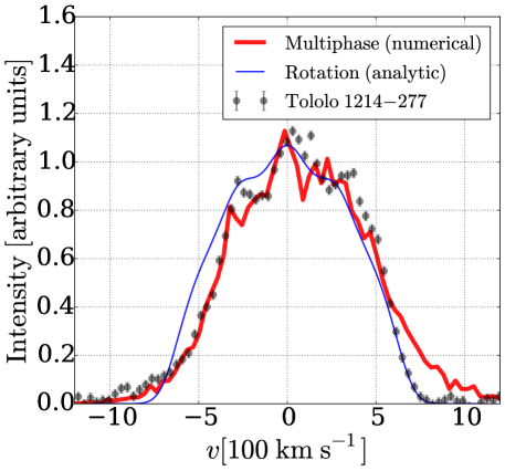
Figure 1: Broad, single peaked and highly symmetric Ly$\alpha$ emission of Tololo 1214-277. Dots correspond to the observational data (Mas-Hesse et al., 2003). The thick red and thin blue curves represent our best fit to the data using the full radiative transfer simulation with a rotation and multiphase model, respectively. These two different models are able to reproduce the main morphological features of Tololo 1214-277’s Ly$\alpha$ line emission.

3.2 Bulk Rotation

The rotation model corresponds to the work presented by Garavito-Camargo et al. (2014) based on the Monte Carlo code CLARA (Forero-Romero et al., 2011). In that model the Ly$\alpha$ photons are propagated within a spherical and homogeneous cloud of HI gas undergoing solid body rotation. The sphere is fully characterized by three parameters: the HI line’s center optical depth $\tau$ measured from the center to its surface, the HI temperature $T$, and the linear surface velocity $V_{\rm max}$. The observed line profile also depends on $\theta$, the angle between the plane perpendicular to the rotation axis and the observational line-of-sight. In this model, dust only changes the overall line normalization and only weakly its shape, i.e. dust cannot change the line symmetry or induce a change in the number of line peaks, moreover it does not change the line width by more than $1\%$ ($5$ km s^-1 in the case of Tololo 1214-277), an effect too small to be observed at the resolution at which we have Tololo 1214-277’s line profile and also negligible compared to the influence of the other free parameters in the model. For these reasons we do not include any dust model.

We use an analytical approximation that captures the most important effects of rotation onto the Ly$\alpha$ line. We defer the reader to Garavito-Camargo et al. (2014) for complete details on the explicit form of this approximation. To fully explore the parameter space we perform Markov Chain Monte Carlo (MCMC) calculations with the emcee Python library (Foreman-Mackey et al., 2013). emcee is an open source optimized implementation of the affine-invariant MCMC sampler (Goodman & Weare, 2010). The algorithm creates a number of walkers that, during a sufficient number of steps, generate parameters’ combinations for a specific model. For each timestep, the code calculates the likelihood of the combination with respect to the observational data. The walkers explore the parameter space sampling the Gaussian likelihood function built as $\propto\exp(-\chi^{2}/2)$, where the $\chi^{2}$ follows the definition in Equation 1. We do not have a closed analytic expression for $\hat{f}$, we compute it by numerical integration of the analytical approximations found in Garavito-Camargo et al. (2014).

We explore flat priors on four parameters: $200<V_{\rm max}/\mathrm{km\ s}^{-1}<600$, $6.0<\log_{10}\tau<9.0$, $4.0<\log_{10}T/10^{4}\mathrm{K}<4.5$ and $0<\theta<90$ using $500$ steps with $24$ walkers for a total of $12000$ points in the chain. Previous exploratory work shows that it is impossible to fit the observed line outside these priors. Finally, we estimate the parameter values from the 16th, 50th and 84th percentiles.

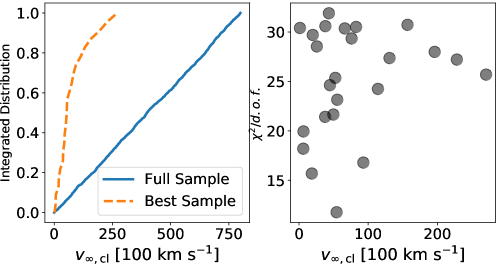
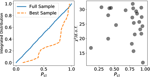
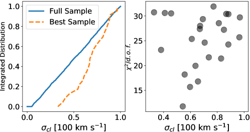
Figure 2: Results from the multiphase model. We only show results for the three parameters with a significant statistical difference between the models with the lowest $\chi^{2}/d.o.f.$ values and its prior distribution. These three parameters are the clump radial velocity at infinity $v_{\infty,\rm{cl}}$; the probability that the Ly$\alpha$ photons were emitted in the clumps, $P_{\rm cl}$; the clump velocity dispersion, $\sigma_{\rm cl}$. The left column corresponds to the parameter’s integrated distributions for models with the lowest $\chi^{2}/d.o.f.$ values (dotted line) compared against the parameter’s prior integrated distributions (continuous line). The right column shows a scatter plot of $\chi^{2}/d.o.f.$ and its corresponding physical parameters. The clump kinematic state is the key ingredient to reproduce Tololo 1214-277’s Ly$\alpha$ line morphology.

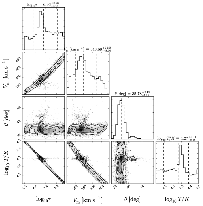
Figure 3: Results from the Markov Chain Monte Carlo computation for the rotation model. The gray scale indicates the point density in parameter space. The dotted vertical lines in the histograms in the diagonal panels represent the 16th, 50th and 84th percentiles. All parameters in the rotation model can be successfully constrained by Tololo 1214-277’s Ly$\alpha$ line morphology to the values written in the top region of the diagonal panels.

4 Results

Figure 1. Summarizes our main finding. Dots represent the observational data for Tololo 1214-277 with the overplot from our best fits from the analytical solution for the multiphase model (thick line) and the rotating homogeneous gas sphere (thin line). The fit to the observations is not perfect. However, in spite of the simplicity of our models, this is the first time that the main features of this SLAE can be reproduced: a broad, highly symmetric, single-peaked Ly$\alpha$ line.

This result does not demonstrate that the kinematic features we include in our models are necessary to reproduce Tololo 1214-277’s features, but at least they show that they are a sufficient condition. This is a significant step forward to understand the influence that different kinematics have in producing the atypical line profile shown by Tololo 1214-277.

In what follows we summarize the values of the kinematic parameters that managed to explain Tololo 1214-277’s Ly$\alpha$ profile.

4.1 Multiphase ISM

With $14$ free parameters our first concern is discovering which parameters matter the most. From the K-S tests we find that only 3 parameters are confidently constrained by Tololo 1214-277’s line shape; $v_{\infty,\rm{cl}}$ (p-value $10^{-18}$), $\sigma_{\rm cl}$ (p-value $10^{-4}$) and $P_{\rm cl}$ (p-value $10^{-4}$).

The low p-values are illustrated by the results shown in Figure 2. Left column shows the difference between the integrated distributions of the full sample (2500 input models) and the $1\%$ models with the lowest $\chi^{2}/d.o.f.$, where we use the total number of degrees of freedom, $d.o.f.=104$. The right column shows the actual $\chi^{2}/d.o.f.$ and its corresponding parameter value. Under these conditions we find $\sigma_{\rm cl}=$$54.3\pm 0.6$ km s^-1, $v_{\infty{\rm,cl}}=$$54.3\pm 5.1$ km s^-1 and $P_{\rm cl}=$$0.96\pm 0.01$, with the minimum $\chi^{2}/d.o.f.=11.7$. This relatively high value for the reduced $\chi^{2}$ could be interpreted as low statistical significance. However, we stress once more that the is the first time that the main features of Tololo 1214-277 can be reproduced, making this model an useful tool to guide the interpretation of complex observational data. These results certainly open up the path to future searches to construct new models.

The results from this model can be qualitatively explained as follows. Due to the large fraction of Ly$\alpha$ photons being emitted within the moving clumps ($P_{\rm cl}\sim 1$) the ‘intrinsic’ profile closely follows the clump kinematics. In other words, the width of the intrinsic line is set by $\sigma_{\mathrm{cl}}$ and its median offset mainly by $v_{\infty,{\rm cl}}$ and $\beta_{\rm cl}$, the exponent defining the steepness of the radial velocity profile. Furthermore, the relatively low mean number of clumps per line of sight, $0.8<f_{\mathrm{cl}}<8$, combined with the high velocity dispersion of the clumps implies existence of low-density inter-clump regions where Ly$\alpha$ photons can freely propagate. This gives result to an emergent spectrum close to the intrinsic one, explaining the high flux at the line’s center.

Because the width of the observable spectrum is hence set primarily by $\sigma_{\rm cl}$, a lower velocity dispersion would produce a narrower line and thus a worse fit. From the lower right panel in Figure 2 we find that in fact it is unlikely that the clump velocity dispersion is lower than $50$ km s^-1.

Having constrained only 3 parameters one might wonder why the other 11 parameters do not seem to matter. In our case this can be explained by the large value of $P_{\rm cl}$ favored by Tololo 1214-277’s observations. A large probability of having Ly$\alpha$  photons emitted in the clumps makes radiative transfer effects, and therefore other parameters such as the clump column density, less relevant for the emergent line profile.

However, we cannot discard that another region of parameter space could also yield a good fit to the observed line-profile. This might be interesting to explore in the future with, e.g., a higher sampling of the parameter space once new observations yield more details on Tololo 1214-277’s kinematic structure.

4.2 Bulk Rotation

The results for this model are easier to interpret due to the fewer number of free parameters and its explicit influence on the semi-analytic solution. The results are summarized in Figure 3. From this analysis we find that the best parameters in the rotation model are a rotational velocity of $V_{\rm max}=348^{+75}_{-48}$ km s^-1, a neutral Hydrogen optical depth of $\log_{10}\tau=6.96^{+0.26}_{-0.18}$, and an inter-stellar medium temperature of $\log_{10}T/\mathrm{K}=4.27^{+0.11}_{-0.18}$. We are also able to constrain the angle between the plane perpendicular to the rotation axis and the observational line-of-sight to $\theta=35.78^{+2.13}_{-1.88}$ degrees. This model cannot reproduce the slight asymmetry present in Tololo 1214-277’s Ly$\alpha$ line; most probably this would require an small amount of outflows, a feature that is not present in the model provided by Garavito-Camargo et al. (2014).

The preferred value for the rotational velocity can be explained as follows. Lower rotational velocities than the favored value would produce a double peaked line as the different doppler shifts produced on different regions of the rotating sphere would not be large enough to smear the double peaks into a single peak (Garavito-Camargo et al., 2014). For the same reason, higher rotation velocities could produce a single peak but the line would be broader than it is observed. The fact that the velocity and optical depth priors were wide enough, allows us to suggest that the current values for the spherical model found by the MCMC are robust given the observational constraints.

5 Discussion

Tololo 1214-277 presents a Ly$\alpha$ emission line with puzzling features. Its flux at the line’s center is high compared to other LAEs at low redshift and the broad, highly symmetrical peak. SLAEs are virtually absent from other LAE surveys at low and high redshift (Yamada et al., 2012; Östlin et al., 2014; Erb et al., 2014; Trainor et al., 2016). Simple shell models fail to reproduce such a spectrum as reported by Verhamme et al. (2015). In the previous sections we show how these characteristics can be explained by two different kinematic models: multiphase ISM and solid body rotation.

Which model could be closer to the actual kinematic conditions in Tololo 1214-277? Integral Field Unit (IFU) observations of other CDGs seem to favor the multiphase model (Cairós et al., 2015; Cairós & González-Pérez, 2017a, b). These observations were performed with the Visible Multi-Object Spectrograph (VIMOS) (Le Fèvre et al., 2003). The spatial sampling was $0.67^{\prime\prime}$ and covered about $30^{\prime\prime}\times 30^{\prime\prime}$ on the sky. They observed nine Blue Compact Galaxies (BCGs) to produce two-dimensional maps of the continuum and prominent emission lines to finally compute velocity field maps using the H$\alpha$ emission line. They find velocity fields ranging from simple rotation patterns (with amplitudes of $10-120$ km s^-1) to highly irregular. The typical velocity dispersion values are in the range $10-50$ km s^-1with the exception of one galaxy that shows a dispersion of $130$ km s^-1.

These results disfavor the high rotational velocity of $V_{m}\sim 350$ km s^-1  that we find in the pure rotation model. On the other hand the results from the multiphase model yield a velocity dispersion $\sigma_{\rm cl}=$$54.3\pm 0.6$ km s^-1, consistent with other observations. We can now estimate a value for the dynamical mass using the constraints for the velocity dispersion, $\sigma$, in a spherical system localized in a region of size $r$

$$M_{\rm dyn}=3\frac{\sigma^{2}r}{G}=3.48\times 10^{9}\left(\frac{\sigma}{100\ \mathrm{km\ s}^{-1}}\right)^{2}\left(\frac{r}{\mathrm{kpc}}\right)M_{\odot}.$$ (2)

Assuming that the Ly$\alpha$ emission is entirely powered by star formation we use the 3D half-light radius $r_{s}=2.25$ kpc as the typical size for the HI region. With $\sigma=\sigma_{\rm{cl}}=$$54.3\pm 0.6$ km s^-1we obtain a dynamical mass of $M_{\rm dyn}=2.31\pm 0.04\times 10^{9}$ $M_{\odot}$, which is ten times the estimated baryonic mass in Tololo 1214-277.

A larger dynamical mass estimate over its baryonic mass hints that Tololo 1214-277 is dark matter dominated. Following the methodology of Tollerud et al. (2011) we estimate that a dark matter halo with a virial mass $\sim 6\times 10^{11}$ M_⊙ and a virial radius $220$ kpc could explain this dynamical mass. This estimate is based on computing the integrated mass profile of a spherical dark matter halo with a Navarro-Frenk-White profile with its concentration following the median mass-concentration relationship found in the Bolshoi simulation (Prada et al., 2012; Poveda-Ruiz et al., 2016). Figure 4 shows the enclosed mass as a function of radius for different dark matter halos together with the Tololo 1214-277’s dynamical mass estimate. This should be considered as an upper bound as lower values could be achieved if one considers instead a cored DM profile. Realistic mass estimates could only be achieved by detailed mass modelling once Tololo 1214-277’s detailed kinematic information becomes available.

New IFU observations are needed to confirm Tololo 1214-277’s kinematics. This could be done with the Multi Unit Spectroscopic Explorer (MUSE) (Bacon et al., 2014), the Gemini Multi-Object Spectrographs (GMOS) (Hook et al., 2004) or the Fibre Large Array Multi Element Spectrograph (FLAMES) (Pasquini et al., 2002) as they have the spatial resolution ($\sim 0.5^{\prime\prime}$), spectral coverage and field of view required to produce H$\alpha$ velocity maps to perform the kind of study presented by Cairós et al. (2015) on CDGs or by Herenz et al. (2016) on nearby Ly$\alpha$  emitting galaxies.

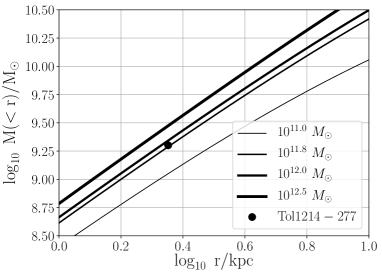
Figure 4: Enclosed mass in a spherical system as a function of radius. Lines correspond to the expectation for dark matter halos following an NFW profile with different virial masses as shown in the legend. The circle corresponds to the dynamical mass estimates for Tololo 1214-277. Under this conditions the dynamical mass estimates for Tololo 1214-277 are consistent with the galaxy being hosted by a dark matter halo of $\sim 6\times 10^{11}$ M_⊙ in mass.

6 Conclusions

In this paper we presented two kinematic models that independently reproduce the so far unexplained observational features of Tololo 1214-277’s Ly$\alpha$ emission line. One model is based on a multiphase ISM with random clump motions and the other on gas bulk solid body rotation. It is the first time that an observed Ly$\alpha$ profile can be reproduced by either of these two kinematic conditions. Our findings highlight the importance of including multiphase and/or rotation conditions as kinematic features to model the Ly$\alpha$ line.

In this particular case, we prefer the multiphase model because it has kinematic conditions similar to other compact dwarf galaxies observed with integral field unit spectroscopy, while the rotational model produces rotational velocities too high for a dwarf galaxy. New IFU observations are the only way to be certain about the detailed kinematic structure in Tololo 1214-277.

All in all, the mere existence of a broad SLAE is interesting. Tololo 1214-277’s line shape is different to others and seems to reveal an unexpected kinematic structure. A confirmation of our results by new observations would support the multiphase model as an element to be included in the study of Ly$\alpha$ emitting galaxies, consolidating the possibility to use the Ly$\alpha$ line to constrain different models of star formation and feedback in the first generation of galaxies.

Appendix A Random Forest Classification

As a complement to the K-S tests on the multiphase data we apply a random forest classification algorithm (James et al., 2014) to find the more relevant parameters in the model to produce a low $\chi^{2}$ result.

We divide the results in two classes: low $\chi^{2}/d.o.f.<35$ and high $\chi^{2}/d.o.f.>35$, that is the limit that divides the best $1\%$ of the models from the rest. The algorithm uses $500$ trees for the classification and a maximum of $3$ depth levels. To check for stability we repeat the computation $10$ times by randomly subsampling the input data to use $80\%$ of the data as the training set.

Figure 5 shows as an example the results for a single classification tree. The tree starts with $28$ and $1962$ models in the low and high $\chi^{2}/d.o.f.$ classes, respectively. In this example the best classification yields $13$ and $44$ models in the low and high $\chi^{2}/d.o.f.$ classes, respectively, after selecting for $v_{\infty,{\rm cl}}<157.0$ km s^-1, $\sigma_{{\rm cl}}>55.6$ km s^-1and $P_{\rm cl}>0.683$.

The results of the random forest classifier over $500$ trees yield that the clump outflow velocity $v_{\infty,\rm{cl}}$, the clump velocity dispersion $\sigma_{\rm cl}$ and the probability that the Ly$\alpha$ emission comes from the clumps $P_{\rm cl}$, are the most influential parameters in finding a model with low $\chi^{2}/d.o.f.$.

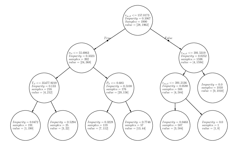
Figure 5: Classification tree example. The aim is to find the parameters that can be used to separate the results in two classes: low $\chi^{2}/d.o.f.<35$ and high $\chi^{2}/d.o.f>35$. Each box describes the condition over the parameter of interest, the level of sample impurity, the total number of samples and the value of the number of samples in each class. In this example we randomly sample $80\%$ of the full data set of models to start with $28$ models in the first class and $1962$ models in the second class; the best way to increase the probability to find a result with low $\chi^{2}/d.o.f.$ ($13$ models, fourth bottom box, from left to the right) is having the clump radial velocity, $v_{\infty,{\rm cl}}<157.0$ km s^-1; the clump velocity dispersion, $\sigma_{{\rm cl}}>55.6$ km s^-1, and the probability to have a Ly$\alpha$ photon emitted in a clump, $P_{\rm cl}>0.683$. The final classification shows that these three are the most relevant to select the best models.

References

- Astropy Collaboration et al. (2013) Astropy Collaboration et al., 2013, A&A, 558, A33
- Bacon et al. (2014) Bacon R., et al., 2014, The Messenger, 157, 13
- Begum et al. (2005) Begum A., Chengalur J. N., Karachentsev I. D., 2005, A&A, 433, L1
- Cairós & González-Pérez (2017a) Cairós L. M., González-Pérez J. N., 2017a, preprint, (arXiv:1708.09407)
- Cairós & González-Pérez (2017b) Cairós L. M., González-Pérez J. N., 2017b, A&A, 600, A125
- Cairós et al. (2015) Cairós L. M., Caon N., Weilbacher P. M., 2015, A&A, 577, A21
- Dey et al. (1998) Dey A., Spinrad H., Stern D., Graham J. R., Chaffee F. H., 1998, ApJ, 498, L93
- Dijkstra (2014) Dijkstra M., 2014, Publ. Astron. Soc. Australia, 31, e040
- Dijkstra & Kramer (2012) Dijkstra M., Kramer R., 2012, MNRAS, 424, 1672
- Dijkstra et al. (2007) Dijkstra M., Lidz A., Wyithe J. S. B., 2007, MNRAS, 377, 1175
- Engelbracht et al. (2008) Engelbracht C. W., Rieke G. H., Gordon K. D., Smith J.-D. T., Werner M. W., Moustakas J., Willmer C. N. A., Vanzi L., 2008, ApJ, 678, 804
- Erb et al. (2014) Erb D. K., et al., 2014, ApJ, 795, 33
- Eskew et al. (2012) Eskew M., Zaritsky D., Meidt S., 2012, AJ, 143, 139
- Foreman-Mackey et al. (2013) Foreman-Mackey D., Hogg D. W., Lang D., Goodman J., 2013, PASP, 125, 306
- Forero-Romero et al. (2011) Forero-Romero J. E., Yepes G., Gottlöber S., Knollmann S. R., Cuesta A. J., Prada F., 2011, MNRAS, 415, 3666
- Fricke et al. (2001) Fricke K. J., Izotov Y. I., Papaderos P., Guseva N. G., Thuan T. X., 2001, AJ, 121, 169
- Garavito-Camargo et al. (2014) Garavito-Camargo J. N., Forero-Romero J. E., Dijkstra M., 2014, ApJ, 795, 120
- Gavilán et al. (2013) Gavilán M., Ascasibar Y., Mollá M., Díaz Á. I., 2013, MNRAS, 434, 2491
- Gawiser et al. (2007) Gawiser E., et al., 2007, ApJ, 671, 278
- Goodman & Weare (2010) Goodman J., Weare J., 2010, Communications in applied mathematics and computational science, 5, 65
- Greig et al. (2013) Greig B., Komatsu E., Wyithe J. S. B., 2013, MNRAS, 431, 1777
- Gronke & Dijkstra (2016) Gronke M., Dijkstra M., 2016, ApJ, 826, 14
- Gronke et al. (2015) Gronke M., Bull P., Dijkstra M., 2015, ApJ, 812, 123
- Harrington (1973) Harrington J. P., 1973, MNRAS, 162, 43
- Hayashino et al. (2004) Hayashino T., et al., 2004, AJ, 128, 2073
- Hayes (2015) Hayes M., 2015, Publ. Astron. Soc. Australia, 32, e027
- Herenz et al. (2016) Herenz E. C., et al., 2016, A&A, 587, A78
- Hook et al. (2004) Hook I. M., Jørgensen I., Allington-Smith J. R., Davies R. L., Metcalfe N., Murowinski R. G., Crampton D., 2004, PASP, 116, 425
- Hummer & Storey (1987) Hummer D. G., Storey P. J., 1987, MNRAS, 224, 801
- Hunter (2007) Hunter J. D., 2007, Computing in Science and Engineering, 9, 90
- Izotov et al. (2004) Izotov Y. I., Papaderos P., Guseva N. G., Fricke K. J., Thuan T. X., 2004, A&A, 421, 539
- James et al. (2014) James G., Witten D., Hastie T., 2014, An Introduction to Statistical Learning: With Applications in R.
- Kennicutt (1998) Kennicutt Jr. R. C., 1998, ARA&A, 36, 189
- Kluyver et al. (2016) Kluyver T., et al., 2016, in ELPUB. pp 87–90
- Kovač et al. (2007) Kovač K., Somerville R. S., Rhoads J. E., Malhotra S., Wang J., 2007, ApJ, 668, 15
- Laursen et al. (2013) Laursen P., Duval F., Östlin G., 2013, ApJ, 766, 124
- Le Fèvre et al. (2003) Le Fèvre O., et al., 2003, in Iye M., Moorwood A. F. M., eds, Proc. SPIEVol. 4841, Instrument Design and Performance for Optical/Infrared Ground-based Telescopes. pp 1670–1681, doi:10.1117/12.460959
- Loeb & Rybicki (1999) Loeb A., Rybicki G. B., 1999, ApJ, 524, 527
- Martin (1998) Martin C. L., 1998, ApJ, 506, 222
- Mas-Hesse et al. (2003) Mas-Hesse J. M., Kunth D., Tenorio-Tagle G., Leitherer C., Terlevich R. J., Terlevich E., 2003, ApJ, 598, 858
- McKee & Ostriker (1977) McKee C. F., Ostriker J. P., 1977, ApJ, 218, 148
- McKinney et al. (2010) McKinney W., et al., 2010, in Proceedings of the 9th Python in Science Conference. pp 51–56
- Mejía-Restrepo & Forero-Romero (2016) Mejía-Restrepo J. E., Forero-Romero J. E., 2016, ApJ, 828, 5
- Neufeld (1991) Neufeld D. A., 1991, ApJ, 370, L85
- Noeske et al. (2003) Noeske K. G., Papaderos P., Cairós L. M., Fricke K. J., 2003, A&A, 410, 481
- Orsi et al. (2008) Orsi A., Lacey C. G., Baugh C. M., Infante L., 2008, MNRAS, 391, 1589
- Orsi et al. (2012) Orsi A., Lacey C. G., Baugh C. M., 2012, MNRAS, 425, 87
- Östlin et al. (2014) Östlin G., et al., 2014, ApJ, 797, 11
- Ott et al. (2005) Ott J., Walter F., Brinks E., 2005, MNRAS, 358, 1453
- Padilla et al. (2010) Padilla N. D., Christlein D., Gawiser E., González R. E., Guaita L., Infante L., 2010, MNRAS, 409, 184
- Partridge & Peebles (1967) Partridge R. B., Peebles P. J. E., 1967, ApJ, 147, 868
- Pasquini et al. (2002) Pasquini L., et al., 2002, The Messenger, 110, 1
- Pedregosa et al. (2011) Pedregosa F., et al., 2011, Journal of Machine Learning Research, 12, 2825
- Pérez & Granger (2007) Pérez F., Granger B. E., 2007, Computing in Science and Engineering, 9, 21
- Poveda-Ruiz et al. (2016) Poveda-Ruiz C. N., Forero-Romero J. E., Muñoz-Cuartas J. C., 2016, ApJ, 832, 169
- Prada et al. (2012) Prada F., Klypin A. A., Cuesta A. J., Betancort-Rijo J. E., Primack J., 2012, MNRAS, 423, 3018
- Pustilnik & Martin (2007) Pustilnik S. A., Martin J.-M., 2007, A&A, 464, 859
- Rivera-Thorsen et al. (2015) Rivera-Thorsen T. E., et al., 2015, ApJ, 805, 14
- Steidel et al. (2010) Steidel C. C., Erb D. K., Shapley A. E., Pettini M., Reddy N., Bogosavljević M., Rudie G. C., Rakic O., 2010, ApJ, 717, 289
- Swaters et al. (2009) Swaters R. A., Sancisi R., van Albada T. S., van der Hulst J. M., 2009, A&A, 493, 871
- Tasitsiomi (2006) Tasitsiomi A., 2006, ApJ, 645, 792
- Tassis et al. (2008) Tassis K., Kravtsov A. V., Gnedin N. Y., 2008, ApJ, 672, 888
- Thuan & Izotov (1997) Thuan T. X., Izotov Y. I., 1997, ApJ, 489, 623
- Tollerud et al. (2011) Tollerud E. J., Bullock J. S., Graves G. J., Wolf J., 2011, ApJ, 726, 108
- Trainor et al. (2016) Trainor R. F., Strom A. L., Steidel C. C., Rudie G. C., 2016, ApJ, 832, 171
- Verhamme et al. (2006) Verhamme A., Schaerer D., Maselli A., 2006, A&A, 460, 397
- Verhamme et al. (2015) Verhamme A., Orlitová I., Schaerer D., Hayes M., 2015, A&A, 578, A7
- Walt et al. (2011) Walt S. v. d., Colbert S. C., Varoquaux G., 2011, Computing in Science & Engineering, 13, 22
- Yamada et al. (2012) Yamada T., Matsuda Y., Kousai K., Hayashino T., Morimoto N., Umemura M., 2012, ApJ, 751, 29