Non-iterative SLAM for Warehouse
Robots Using Ground Textures

Abstract

We present a novel visual SLAM method for the warehouse robot with a single downward-facing camera using ground textures. Traditional methods resort to feature matching or point registration for pose optimization, which easily suffers from repetitive features and poor texture quality. In this paper, we present a robust kernel cross-correlator for robust image-level registration. Compared with the existing methods that often use iterative solutions, our method, named non-iterative visual SLAM (NI-SLAM), has a closed-form solution with a complexity of $\mathcal{O}(n\log n)$. This allows it to run very efficiently, yet still provide better accuracy and robustness than the state-of-the-art methods. In the experiments, we demonstrate that it achieves 78% improvement over the state-of-the-art systems for indoor and outdoor localization. We have successfully tested it on warehouse robots equipped with a single downward camera, showcasing its product-ready superiority in a real operating area.

I Introduction

Visual Simultaneous Localization and Mapping (SLAM) is a pivotal task in robotics, with substantial implications for various applications, including unmanned aerial vehicles and autonomous driving [1]. Despite significant advancements, visual SLAM continues to face challenges, particularly in extreme scenarios, e.g., , illumination changes [2], the presence of dynamic objects [3], and large-scale environments [4].

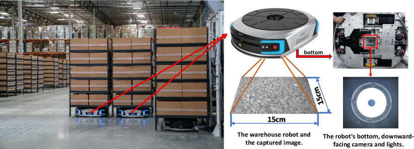
Consequently, when deploying visual SLAM in warehouse robots, numerous hurdles must be overcome. On one hand, in environments like the one illustrated in Fig. 1, where multiple robots collaborate to transport goods within the warehouse, the high dynamism often leads to visual localization errors. On the other hand, warehouses are typically vast, causing static features to be distant from the camera and reducing visual SLAM system accuracy. As a result, tag-based localization continues to be the predominant technique for warehouse use cases. This involves placing a multitude of QR codes on the floor and utilizing a camera positioned downward to detect them for localization purposes. However, accurately positioning these QR codes is a time-consuming process, often taking several weeks or even months. Additionally, other sensors, such as inertial measurement units (IMUs) and wheel odometry, are still necessary to provide localization between consecutive QR codes. Any drift error in these sensors can lead to the failure to detect the next QR code, especially when it is close to the ground and has a narrow field of view.

To enhance the reliability and adaptability of localization, several systems have chosen to adopt ground texture-based localization using downward-facing cameras [5, 6, 7, 8, 9]. These systems detect numerous ground image features and use point-level feature matching to determine the robot’s pose. However, point-level matching relies on the availability of an adequate number of distinctive features, which may not always be guaranteed, particularly when dealing with ground textures with repetitive local patterns or a scarcity of identifiable corners. Therefore, there is a pressing necessity for the development of strategies that go beyond point-level matching to enhance the robustness of ground-texture-based visual SLAM algorithms.

Figure 1: In the warehouse, dynamic objects (robots and storage racks) and large-scale environments make the localization with a forward-facing camera or LiDAR very challenging, so currently, a downward-facing camera is usually used to detect tags deployed on the ground for stable localization. To eliminate this limitation, we developed a non-iterative SLAM for warehouse robots. It provides robust localization with 78% improvements over the state-of-the-art (SOTA) SLAM systems on various ground textures.

Motivated by these observations, we argue that ground-texture-based visual SLAM systems can benefit from image-level matching. This is because (1) image-level matching is not dependent on the presence of frequent corners or textures, making it robust against low-texture environments and image blurriness and (2) image-level matching can seamlessly connect dominant patterns using comprehensive global information, preventing the system from losing track on the ground when dealing with repetitive local patterns. Despite those appealing properties, the direct implementation of image matching in visual SLAM for warehouse robots presents challenges. This complication arises because current image-level matching approaches either lack efficiency, as evidenced by studies such as CodeSLAM [10], SceneCode [11], and DytanVO [12], or are incapable of accurately estimating image rotation, as indicated in the research conducted by MKCF [13] and DSST [14].

To address these issues, we present a novel approach called the Kernel Cross-Correlator (KCC) and designed to efficiently estimate geometric transformation in images. Unlike current solutions that necessitate feature detection, matching, and an iterative optimization for pose estimation, KCC conducts image-level matching and calculates the camera’s pose through a non-iterative closed-form solution, resulting in exceptional efficiency. Therefore, we named our method “Non-Iterative SLAM (NI-SLAM)”. In summary, our contributions include

• We propose a novel visual SLAM pipeline for warehouse robots using ground textures, which includes non-iterative visual odometry, loop closure detection, and map reuse. Our system can provide robust pose estimation and localization in dynamic and large-scale environments using only a single downward-facing camera.

• We introduce kernel cross-correlators into the SLAM systems for image transform estimation, which provides reliable camera pose estimation for both visual odometry and loop closure detection. It has a closed-form solution of complexity $\mathcal{O}(n\log n)$, where $n$ is the number of pixels, hence it is very efficient and can run in real-time while consuming few computing resources, which is crucial for low-power robotic applications.

• We collect and release a ground texture dataset for ground-texture-based localization which contains 10 different kinds of textures. As far as we know, it is the first publicly available ground texture dataset with accurate ground truth.

• We perform extensive experiments that prove the efficiency and effectiveness of the proposed methods. The results show that NI-SLAM achieves 78% improvements over the state-of-the-art (SOTA) systems on various ground textures. We release the source code and data at https://github.com/sair-lab/ni-slam to benefit the community.

This paper is an extension of our conference paper [15, 16, 17]. The preliminary version [15] is only designed for RGB-D-inertial odometry since it used the kernelized correlation filter (KCF) [18], which can only predict image translation. In this version, we have substantial improvements, including

• We develop a rigorous and detailed proof for our proposed KCC, which is able to estimate any image transformation beyond translation, including rotation and scale. This makes NI-SLAM compatible with other sensor settings such as a single downward-facing camera.

• We introduce a loop closure detection module by applying KCC to historical key-frames. We also add an online mapping module with pose graph optimization. This forms a complete visual SLAM system.

• We design a map reuse module, where a prior ground texture map can be built using the proposed visual SLAM system or any other localization methods, then the robot can use the map for drift-free re-localization.

• We conduct extensive experiments for warehouse robot localization. It shows that NI-SLAM is able to provide reliable localization compared to state-of-the-art algorithms.

The remainder of this article is organized as follows. In Section II, we review the related works on the ground-texture-based localization, image-level matching methods and the correlation filter. In Section III, we present the kernel cross-correlator with a detailed proof to estimate the relative transformation between two images. Based on KCC, a ground-texture-based visual SLAM system is designed in Section IV. We present the experimental results in Section V to verify the robustness of NI-SLAM compared with the SOTA systems. This article is concluded with limitations in Section VI.

II Related work

Our NI-SLAM introduces a new non-linear correlation filter for image matching in the SLAM system using ground textures, thus the related work on ground-texture-based localization systems, image-level matching, and correlation filters will be summarized in Section II-A, II-B, and II-C, respectively.

II-A Ground Texture-based Localization

II-A1 Feature-based Methods

Most ground-texture-based visual localization systems are based on feature detection, matching and iterative 3-DOF pose estimation. Ranger [5] detects CenSurE [19] features on the road surfaces and matches them using ORB [20] descriptors. Then a coarse homography is computed with RANSAC to discard false matches. Finally, a fine 2D pose is estimated using the remaining correspondences. StreepMap [6] proposes two algorithms and names them feature-based approach and line-based approach, respectively. The first approach detects SURF [21] features and tracks them with Lucas-Kanade method[22]. The second approach fuses the measurements from line features and an IMU together using an Extended Kalman Filter (EKF). Micro-GPS [8] uses the SIFT scale-space DoG detector and gradient orientation histogram descriptor [23] for both mapping and localization.

Schmid et al. [9] improve Micro-GPS by proposing identity feature matching, where only identical descriptors are considered as matches. Then they extend this work by replacing SIFT feature detection with randomly sampled points [9]. Zhang et al. [24] design a Convolutional Neural Network (CNN) to detect feature points on the ground texture image. Kyle et al. [25] propose ground texture SLAM, where ORB features are detected and matched using Fast Library for Approximate Nearest Neighbors (FLANN) method [26]. A factor graph is constructed and optimized to estimate the transformation between adjacent frames. To correct the drift error, they train a vocabulary tree using Bag of Words (BoW) library [27] to find loop closures. As far as we know, ground texture SLAM is the latest state-of-the-art ground-texture-based localization system, and it has opened the source code, so we take it as the most important baseline in the experiments.

II-A2 Correction-Based Methods

Kelly et al. [28] analyze the eigenvalues of a matrix composed of image intensity gradients from the input image, aiming to detect areas with bidirectional texture. Then small patches ($25\times 25$ pixel) around these points are selected as features and matched using cross-correlation. Munir Zaman [29] estimates the transformation between two images by finding the maximum peak of their cross-correlations. The system needs an accurate prior rotation with the error within $2^{\circ}$. Then he transforms the second image with a set of rotations and translations and computes their cross-correlations with the first image. The transformation with the maximum peak is regarded as the true one. Similar methods are also used in [30] and [31]. These two systems employ template matching and cross-correlation to estimate the 3-DOF relative pose between two frames. Nagai et al. [32] detect two groups of points for each image, and then use a conventional template matching to find the correction of points on different frames.

II-A3 Datasets

To the best of our knowledge, only two ground texture datasets for localization are publicly available. One is the Micro-GPS dataset [8] and the other is the HD Ground dataset [33]. The authors of the Micro-GPS dataset collect data on 7 kinds of ground textures. Their imaging system consists of a Point Grey CM3 grayscale camera pointed downwards at the ground and surrounded by a set of LED lights. For each kind of texture, both databases for mapping and test sequences for localization are collected. The HD Ground dataset contains 11 kinds of ground textures. Similarly, the data is collected by a ground-facing camera. The recording area is shielded from external lighting and illuminated by a 24V, 72Watt LED ring. However, the ground truths of these two datasets are both from image stitching instead of high-precision pose measurement devices, so their accuracy highly depends on the performance of feature detection and matching of the image-stitching system.

II-B Image- and Scene-Level Matching

KinectFusion [34] applies a coarse-to-fine iterative closet point (ICP) algorithm with geometric constraints to track the live depth frame relative to the global model. ElasticFusion [35] combines dense geometric constraints with photometric constraints to achieve robust pose estimation. In [36], pose estimation is obtained by a dense every-frame volumetric fusion front-end, and the dense surface is corrected by a non-rigid map deformation back-end. DynamicFusion [37] generalizes the truncated signed distance function to nonrigid case, so that dynamic scenes can be reconstructed and a volumetric 6-D motion field can be estimated. CodeSLAM [10] introduces a dense representation of scene geometry which generates codes from an auto-encoder. SceneCode [11] introduces a new compact and optimizable semantic representation by training a variational auto-encoder that is conditioned on a color image.

II-C Correlation Filter

Correlation filter is a class of classifier, which is specifically optimized to produce sharp peaks in the output to achieve accurate localization of targets [38]. By specifying the desired response at every location, the average synthetic exact filter (ASEF) generalizes across the entire training set by averaging multiple exact filters [39]. To overcome the overfitting problem of ASEF, the minimum output sum of squared error (MOSSE) filter adds a regularization term and introduces it into visual tracking [40]. Its superior speed and robustness ignited the boom and development of CF-based tracking. Kernelized correlation filter (KCF) brings circulant training structure into kernel ridge regression [18]. This enables learning with element-wise operation instead of costly matrix inversion, providing much more robustness while still with reasonable learning speed. Multi-kernel correlation filter (MKCF) [13] extends KCF to multiple kernels, which further improves the accuracy.

To alleviate the boundary effect of CFs, zero aliasing correlation filter (ZACF) [41] introduces the zero-aliasing constraints and provides both closed-form and iterative proximal solutions by ensuring that the optimization criterion for a given CF corresponds to a linear correlation rather than a circular correlation. However, it requires heavy computation and is not suitable for real-time applications. Discriminative scale space tracking (DSST) [14] is proposed to learn multiple MOSSE on different scales, enabling estimation of both translation and scale at the cost of repeated calculations of MOSSE. STRCF [42] introduced temporal regularization to spatially regularized correlation filters. Spatially local response map variation is introduced in [43] as spatial regularization to make the correlation filter focus on the trustworthy parts of the object.

III Kernel Cross-Correlator

The core of our ground-texture-based localization system is to estimate the relative transformation, encompassing translation and rotation movements, between two images. Therefore, prior to delving into the architecture of our system, we present the kernel cross-correlator for image transformation estimation, aiming to provide a clearer understanding. Given a key-frame $\mathbf{z}\in\mathbb{R}^{M\times N}$ and a current image $\mathbf{x}\in\mathbb{R}^{M\times N}$, our objective is to find a transformation $\mathcal{T}:\mathbb{R}^{M\times N}\mapsto\in\mathbb{R}^{M\times N}$, so that the transformed key-frame $\mathcal{T}(\mathbf{z})$ has the maximum kernel similarity with the current image $\mathbf{x}$:

$$\mathcal{T}^{\star}=\arg_{\mathcal{T}}\max\bm{\kappa}\left(\mathbf{x},\mathcal{T}(\mathbf{z})\right)$$ (1)

where $\bm{\kappa}:\mathbb{R}^{M\times N}\times\mathbb{R}^{M\times N}\mapsto\mathbb{R}^{+}$ is a robust kernel function to measure the similarity of two signals. In this paper, the image transformation $\mathcal{T}$ can be translation, rotation, or both.

One of the widely used solutions to the objective function (1) is to optimize the kernel function with respect to the images via gradient descent. However, this is often computationally heavy and the objective function (1) has multiple local minimums, leading to its sensitivity to initialization. We next show that the objective function (1) can be easily solved via our kernel cross-correlator in a computational complexity of $\mathcal{O}(n\log n)$, where $n=MN$ is the number of pixels.

III-A Kernel Cross-Correlation

Our fundamental insight is that if we can compute the kernel functions for every potential transformation $\mathcal{T}_{i}$ within $\mathcal{T}$, then the solution to (1) is just the transformation corresponding to the highest kernel function value. In this context, we have

$$\mathcal{T}^{\star}=\arg_{\mathcal{T}}\max\left(\kappa(\mathbf{x},\mathcal{T}_{0}(\mathbf{z})),\cdots,\kappa(\mathbf{x},\mathcal{T}_{m-1}(\mathbf{z})\right),$$ (2)

where $\mathbf{z}_{i}=\mathcal{T}_{i}(\mathbf{z})$ is a transformation of $\mathbf{z}$. For the sake of simplicity, we denote images as vectorized signals $\mathbf{z,x}\in\mathbb{R}^{n}$, where $n=MN$. The derived results can be easily extended to the matrix case. Note that the index starts from 0 to denote no transformation, which is also compatible with the source code. Define the kernel vector as $\bm{\kappa}_{\mathbf{z}}(\mathbf{x})=[\kappa(\mathbf{x},\mathcal{T}_{0}(\mathbf{z})),\cdots,\kappa(\mathbf{x},\mathcal{T}_{m-1}(\mathbf{z})]^{T}$, then our kernel cross-correlation (KCC) is defined as

$$\mathbf{g}(\mathbf{x})=\bm{\kappa}_{\mathbf{z}}(\mathbf{x})\otimes\mathbf{h},$$ (3)

where $\otimes$ is the linear circular cross-correlation operator [44], and $\mathbf{h}\in\mathbb{C}^{m}$ is an unknown correlator to be estimated, and $\mathbf{g}\in\mathbb{C}^{m}$ is the correlation output. Due to the cross-correlation theorem [44], KCC (3) can be calculated in frequency domain:

$$\hat{\mathbf{g}}(\mathbf{x})=\hat{\bm{\kappa}}_{\mathbf{z}}(\mathbf{x})\odot\hat{\mathbf{h}}^{*},$$ (4)

where $\odot$ is the element-wise multiplication, $\cdot^{*}$ is the complex conjugate, and $\hat{\cdot}$ is the fast Fourier transform (FFT) denoted by $\mathcal{F}(\cdot)$. The background of the linear cross-correlation and cross-correlation theorem can be found in Appendix A.

Before delving further, we will first define equivariance for clearer comprehension and then demonstrate that KCC is equivariant to any transformations, which is an important property we leverage for pose estimation in NI-SLAM system.

Lemma 1 (Equivariance [45]).

Consider a function $\mathbf{f}$ and a transformation $\mathcal{T}$, the function $\mathbf{f}$ is equivariant to $\mathcal{T}$ if

$$\mathbf{f}(\mathcal{T}(\mathbf{x}))=\mathcal{T}^{\prime}(\mathbf{f}(\mathbf{x}))$$ (5)

for all input $\mathbf{x}$, where $\mathcal{T}^{\prime}$ might be the same as $\mathcal{T}$ or another related transformation. In simple terms, a function is said to be equivariant if when the input changes in a certain way, the output changes in a predictable and corresponding manner.

Theorem 2 (KCC Equivariance).

Kernel cross-correlator in (3) is equivariant to transformation $\mathcal{T}_{i}$, if $\mathcal{T}_{i}$ is periodical: $\mathcal{T}_{i}(\mathbf{x})=\mathcal{T}_{i+m}(\mathbf{x})$, where $m$ is the period. In other words,

$$\mathbf{g}(\mathcal{T}_{i}(\mathbf{x}))=\bm{\kappa}_{\mathbf{z}}(\mathcal{T}_{i}(\mathbf{x}))\otimes\mathbf{h}=(\bm{\kappa}_{\mathbf{z}}(\mathbf{x})\otimes\mathbf{h})_{(i)}=\mathbf{g}_{(i)}(\mathbf{x}),$$ (6)

where $\cdot_{(i)}$ denotes the circular translated vector by $i$ elements.

Proof.

Recollect that circular translation is a periodical transform function and cross-correlation is equivariant to circular translation [45], this means that $(\mathbf{a}\otimes\mathbf{b})_{(i)}=\mathbf{a}_{(i)}\otimes\mathbf{b}$, where $\mathbf{a},\mathbf{b}$ are two random vectors. Assume $\mathbf{g}^{\prime}=\bm{\kappa}_{\mathbf{z}}(\mathcal{T}_{j}(\mathbf{x}))\otimes\mathbf{h}$, then

$$\mathbf{g}^{\prime}=[\kappa(\mathcal{T}_{j}(\mathbf{x}),\mathcal{T}_{0}(\mathbf{z})),\cdots,\kappa(\mathcal{T}_{j}(\mathbf{x}),\mathcal{T}_{m-1}(\mathbf{z}))]\otimes\mathbf{h}.$$ (7)

Since $\mathcal{T}_{j}$ is periodical, we have

$$\bm{\kappa}_{\mathbf{z}}(\mathcal{T}_{j}(\mathbf{x}))=(\bm{\kappa}_{\mathbf{z}}(\mathbf{x}))_{(j)}.$$ (8)

This means that

$$\bm{\kappa}_{\mathbf{z}}(\mathcal{T}_{j}(\mathbf{z}))\otimes\mathbf{h}=(\bm{\kappa}_{\mathbf{z}}(\mathbf{z}))_{(j)}\otimes\mathbf{h}=(\bm{\kappa}_{\mathbf{z}}(\mathbf{z})\otimes\mathbf{h})_{(j)},$$ (9)

which completes the proof. ∎

In the above proof, we show that the transformation $\mathcal{T}$ should be periodic like rotation. However, this isn’t always a practical necessity. For example, image translation doesn’t strictly follow circular translation, leading to a boundary effect as mentioned in [40]. Nevertheless, the boundary effect can be diminished by applying a Gaussian mask to the image, as demonstrated by [18]. This paper doesn’t delve into addressing the boundary effect for KCC since there are alternative strategies available, like the one presented in [41]. Indeed, we’ve established that KCC is equivariant to any transformation such as translation, rotation, and scale transformation in [16]. However, the primary emphasis of this paper is its capability to estimate the translation and rotation of ground-texture images.

III-B The Closed-form Solution to KCC

The basic idea to estimate image transformation using KCC is that we can take advantage of the equivariance property to convert the effect of a transformation into the translation of its output. Concretely, if we can find a correlation filter $\mathbf{h}^{\star}$, that is able to map the kernel vector $\bm{\kappa}_{\mathbf{z}}(\mathbf{z})$ to a predefined correlation output $\mathbf{g}^{\star}:=\bm{\kappa}_{\mathbf{z}}(\mathbf{z})\otimes\mathbf{h}^{\star}$, then the best transformation of $\mathbf{x}$ denoted as $\mathcal{T}^{\star}(\mathbf{x})$ is corresponding to the translation of $\bm{\kappa}_{\mathbf{z}}(\mathbf{x})\otimes\mathbf{h}^{\star}$ relative to the predefined target $\mathbf{g}^{\star}$.

For simplify, we can set $\mathbf{g}^{\star}$ as a single peak vector, then the translation of $\bm{\kappa}_{\mathbf{z}}(\mathbf{x})\otimes\mathbf{h}^{\star}$ relative to $\mathbf{g}^{\star}$ can be found by calculating the translation between their maximum values:

$$\begin{matrix}[l]&i^{\star}&=&\arg_{i}\max\mathbf{g}^{\star}[i],\\ &j^{\star}&=&\arg_{j}\max\left(\bm{\kappa}_{\mathbf{z}}(\mathbf{x})\otimes\mathbf{h}^{\star}\right)[j],\\ &\mathcal{T}^{\star}&=&\mathcal{T}_{(j^{\star}-i^{\star})\%m},\end{matrix}$$ (10)

where $\%$ is the modulo operator.

In this way, our problem becomes how to find the correlator $\mathbf{h}^{\star}$ satisfying $\mathbf{g}^{\star}=\bm{\kappa}_{\mathbf{z}}(\mathbf{z})\otimes\mathbf{h}^{\star}$. Intuitively, it can be solved by finding the optimal solution to the function:

$$\min_{\mathbf{h}}\|\bm{\kappa}_{\mathbf{z}}(\mathbf{z})\otimes\mathbf{h}-\mathbf{g}^{\star}\|^{2}+\lambda\|\mathbf{h}\|^{2}.$$ (11)

where the second term is a regularization to prevent overfitting. However, objective function (11) is difficult to solve and has high computational complexity. Inspired by the fact that cross-correlation can be accelerated in frequency domain, we instead minimize its alternative function in frequency domain to take advantage of the efficient element-wise operation:

$$\min_{\hat{\mathbf{h}}^{*}}\|\hat{\bm{\kappa}}_{\mathbf{z}}(\mathbf{z})\odot\hat{\mathbf{h}}^{*}-\hat{\mathbf{g}}^{\star}\|^{2}+\lambda\|\hat{\mathbf{h}}^{*}\|^{2},$$ (12)

where $\hat{\mathbf{g}}^{\star}:=\mathcal{F}(\mathbf{g}^{\star})$ and $\hat{\mathbf{h}}^{*}:=\mathcal{F}^{*}(\mathbf{h})$ are the corresponding FFT of $\mathbf{g}$ and $\mathbf{h}$ to simplify the notations.

Our motivation of using the objective function (12) instead of (11) is that (12) has the following efficient closed-form solution in frequency domain, which is vital for real-time systems.

Theorem 3 (KCC).

There is a closed-form solution to the objective function (12) for kernel cross-correlator (4),

$$\hat{\mathbf{h}}^{*}=\frac{\hat{\mathbf{g}}^{\star}\odot\hat{\bm{\kappa}}^{*}_{\mathbf{z}}(\mathbf{z})}{\hat{\bm{\kappa}}^{*}_{\mathbf{z}}(\mathbf{z})\odot\hat{\bm{\kappa}}_{\mathbf{z}}(\mathbf{z})+\lambda},$$ (13)

where the operator $\frac{\cdot}{\cdot}$ denotes the element-wise division and $\hat{\mathbf{h}}^{*}$ is the conjugate of Fourier transform of $\mathbf{h}^{\star}$.

Proof.

Without ambiguity, we will denote $\mathbf{g}^{\star}$ as $\mathbf{g}$ in this proof for simplicity. To solve the optimization problem (12), we set its first derivative with respect to $\hat{\mathbf{h}}^{*}$ to zero, i.e.,

$$\frac{\partial}{\partial\hat{\mathbf{h}}^{*}}\left(\|\hat{\bm{\kappa}}_{\mathbf{z}}(\mathbf{z})\odot\hat{\mathbf{h}}^{*}-\hat{\mathbf{g}}\|^{2}+\lambda\|\hat{\mathbf{h}}^{*}\|^{2}\right)=0.$$ (14)

Then by calculating the complex square ($\|a\|^{2}=aa^{*}$), we have

$$\frac{\partial}{\partial\hat{\mathbf{h}}^{*}}\Bigg{(}\hat{\bm{\kappa}}_{\mathbf{z}}(\mathbf{z})\odot\hat{\mathbf{h}}^{*}\odot\hat{\bm{\kappa}}^{*}_{\mathbf{z}}(\mathbf{z})\odot\hat{\mathbf{h}}-\hat{\bm{\kappa}}_{\mathbf{z}}(\mathbf{z})\odot\hat{\mathbf{h}}^{*}\odot\hat{\mathbf{g}}^{*}$$ (15)

$$-\hat{\mathbf{g}}\odot\hat{\bm{\kappa}}^{*}_{\mathbf{z}}(\mathbf{z})\odot\hat{\mathbf{h}}+\hat{\mathbf{g}}\odot\hat{\mathbf{g}}^{*}+\lambda\hat{\mathbf{h}}^{*}\odot\hat{\mathbf{h}}\Bigg{)}=0$$

We next obtain the derivative with respect to $\hat{\mathbf{h}}^{*}$ by taking $\hat{\mathbf{h}}$ as an independent variable of $\hat{\mathbf{h}}^{*}$, thus we have

$$0=\hat{\bm{\kappa}}_{\mathbf{z}}(\mathbf{z})\odot\hat{\bm{\kappa}}^{*}_{\mathbf{z}}(\mathbf{z})\odot\hat{\mathbf{h}}-\hat{\bm{\kappa}}_{\mathbf{z}}(\mathbf{z})\odot\hat{\mathbf{g}}^{*}+\lambda\hat{\mathbf{h}}$$ (16)

Therefore, we can obtain $\hat{\mathbf{h}}$ as

$$\hat{\mathbf{h}}=\frac{\hat{\bm{\kappa}}_{\mathbf{z}}(\mathbf{z})\odot\hat{\mathbf{g}}^{*}}{\hat{\bm{\kappa}}_{\mathbf{z}}(\mathbf{z})\odot\hat{\bm{\kappa}}_{\mathbf{z}}^{*}(\mathbf{z})+\lambda}.$$ (17)

Due to the properties of the complex conjugate, i.e., $a^{*}\cdot b^{*}=(a\cdot b)^{*}$, $a^{*}/b^{*}=(a/b)^{*}$, and $a^{*}+b^{*}=(a+b)^{*}$, the solution (13) can be obtained from (17) by taking the conjugate on both sides, which completes the proof. ∎

Theorem 3 indicates that we can calculate a correlator $\hat{\mathbf{h}}^{*}$ for every key-frame, and then predict the transformation of any image $\mathbf{x}$ relative to the key-frame via (10). This can be used for both visual odometry and loop closure detection.

In practice, the solution (13) can be further simplified. For example, we can add a weighted regularization to the objective function (18), which results in a weighted regularized KCC:

$$\min_{\hat{\mathbf{h}}^{*}}\|\hat{\bm{\kappa}}_{\mathbf{z}}(\mathbf{z})\odot\hat{\mathbf{h}}^{*}-\hat{\mathbf{g}}\|^{2}+\lambda\|\sqrt{\hat{\bm{\kappa}}_{\mathbf{z}}(\mathbf{z})}\odot\mathbf{h}\|^{2}.$$ (18)

Theorem 4 (Weighted Regularized KCC).

There is a closed-form solution to the objective function (18) for KCC (4), i.e.,

$$\hat{\mathbf{h}}^{*}=\frac{\hat{\mathbf{g}}^{\star}}{\hat{\bm{\kappa}}_{\mathbf{z}}(\mathbf{z})+\lambda}.$$ (19)

Proof.

Since only the regularization of the objective function is changed, the solution to (18) can be obtained by updating the regularization term of (17), hence we have

$$\hat{\mathbf{h}} =\frac{\hat{\mathbf{g}}^{*}\odot\hat{\bm{\kappa}}_{\mathbf{z}}(\mathbf{z})}{\hat{\bm{\kappa}}_{\mathbf{z}}(\mathbf{z})\odot\hat{\bm{\kappa}}_{\mathbf{z}}^{*}(\mathbf{z})+\lambda\hat{\bm{\kappa}}_{\mathbf{z}}(\mathbf{z})},$$ (20)

$$=\frac{\hat{\mathbf{g}}^{*}}{\hat{\bm{\kappa}}^{*}_{\mathbf{z}}(\mathbf{z})+\lambda}.$$

Similarly, solution (19) can be obtained by taking the conjugate on both sides, which completes the proof. ∎

Therefore, we have the following theorem to estimate the transformation between two signals, if we set the correlation target as a single peak binary vector located at the first element.

Theorem 5.

The transformation between two signals $\mathbf{x},\mathbf{z}\in\mathbb{R}^{n}$ can be estimated in terms of the minimum squared spectrum error (18), i.e., $\mathbf{x}=\mathcal{T}^{\star}(\mathbf{z})$ via KCC as

$$\mathcal{T}^{\star}=\mathcal{T}_{j^{\star}},$$ (21)

where

$$j^{\star}=\arg_{j}\max\mathcal{F}^{-1}[j]\left(\frac{\hat{\mathbf{g}}^{\star}\odot\hat{\bm{\kappa}}_{\mathbf{z}}(\mathbf{x})}{\hat{\bm{\kappa}}_{\mathbf{z}}(\mathbf{z})+\lambda}\right),$$ (22)

if $\mathbf{g}^{\star}$ is the correlation target and is predefined as

$$\mathbf{g}^{\star}[i]=\left\{\begin{matrix}[l]1&i=0\\ 0&i=1,2,\cdots,m-1\end{matrix}\right..$$ (23)

Proof.

Substitute (19) into (4), then we can obtain (22) by taking $i^{\star}=0$ in (10) because of $0=\arg_{i}\max\mathbf{g}^{\star}[i]$ in (23). ∎

Estimation Confidence

Due to the boundary effect and noises, we cannot obtain the same correlation output defined in (23), however, we are able to estimate its confidence from its peakness. In the experiments, we use the peak-to-sidelobe ratio [18] to calculate the estimation confidence.

$$P_{s}(\mathbf{x})=\frac{\max\mathbf{g}(\mathbf{x},\mathbf{h}^{\star})-\mu_{s}(\mathbf{g}(\mathbf{x},\mathbf{h}^{\star}))}{\delta_{s}(\mathbf{g}(\mathbf{x},\mathbf{h}^{\star}))},$$ (24)

where $\mu_{s}$ and $\delta_{s}$ are the mean and standard deviation of the sidelobe, which is the output $\mathbf{g}(\mathbf{x},\mathbf{h}^{\star})$ excluding the peak.

Figure 2: An illustration of motion estimation with the proposed KCC. Two input images are represented as $\mathbf{z}$ and $\mathbf{x}$ respectively. The output rotation $\mathbf{\theta}$ and translation $\mathbf{t}$ are estimated in a decoupled way.

Figure 3: The pipeline of NI-SLAM. It is a ground-texture-based, non-iterative visual SLAM system. The rotation and translation are decoupled and estimated using kernel cross-correctors. A map is maintained to store the key-frames for loop closure detection and loop correction.

III-C Kernel Vector

Although we have shown that any transformation can be estimated in Theorem 5 with KCC, the calculation of the kernel vectors $\hat{\bm{\kappa}}_{\mathbf{z}}(\mathbf{x})$ are still the bottleneck. We next show that the kernel vector $\bm{\kappa}_{\mathbf{z}}(\mathbf{x})$ can also be computed in the frequency domain for acceleration. Without loss of generality, we will take the Gaussian kernel as an example, thus we have the $i^{\text{th}}$ element of the kernel vector as

$$\bm{\kappa}_{\mathbf{z}}(\mathbf{x})[i] =e^{-\frac{1}{2}\|\mathbf{x}-\mathcal{T}_{i}(\mathbf{z})\|}$$ (25)

$$=e^{\mathbf{x}^{T}\mathcal{T}_{i}(\mathbf{z})-\frac{1}{2}\|\mathbf{x}\|^{2}-\frac{1}{2}\|\mathcal{T}_{i}(\mathbf{z})\|^{2}}.$$

Since calculating $\|\mathcal{T}_{i}(\mathbf{z})\|^{2}$ has a complexity of $\mathcal{O}(n)$, the entire kernel vector $\bm{\kappa}_{\mathbf{z}}(\mathbf{x})$ requires a complexity of $\mathcal{O}(n^{2})$. We next proceed to demonstrate that this computation can be sped up in the frequency domain to a complexity of $\mathcal{O}(n\log n)$.

III-C1 Translation

Assume $\mathcal{T}_{i}(\mathbf{z})$ is a circular translation, i.e., $\mathcal{T}_{i}(\mathbf{z})=\mathbf{z}_{(i)}$, then the kernel vector is $\bm{\kappa}_{\mathbf{z}}(\mathbf{x})=[\kappa(\mathbf{x},\mathbf{z}_{(0)}),\cdots,\kappa(\mathbf{x},\mathbf{z}_{(m-1)})]^{T}$. For each element in the kernel vector, we can take out the common items, then

$$\bm{\kappa}_{\mathbf{z}}(\mathbf{x}) =e^{-\frac{1}{2}\|\mathbf{x}\|^{2}-\frac{1}{2}\|\mathbf{z}\|^{2}}\cdot e^{{\big{[}\mathbf{x}^{T}\mathbf{z}_{(0)},~{}\cdots,~{}\mathbf{x}^{T}\mathbf{z}_{(m-1)}\big{]}}^{T}},$$ (26)

$$=e^{-\frac{1}{2}\|\mathbf{x}\|^{2}-\frac{1}{2}\|\mathbf{z}\|^{2}}\cdot e^{\mathbf{x}\otimes\phi(\mathbf{z})},$$

where $\|\mathbf{z}\|^{2}=\|\mathbf{z}_{(i)}\|^{2}$ due to the circular translation property. Therefore, the kernel vector includes another cross-correlation which can be computed in the frequency domain

$$\bm{\kappa}_{\mathbf{z}}(\mathbf{x}) =e^{-\frac{1}{2}\|\mathbf{x}\|^{2}-\frac{1}{2}\|\mathbf{z}\|^{2}}\cdot e^{\mathcal{F}^{-1}\big{(}\hat{\mathbf{x}}\odot\hat{\mathbf{z}}\big{)}},$$ (27)

of which the complexity is reduced to $\mathcal{O}(n\log n)$ from $\mathcal{O}(n^{2})$. The sum of squares can also be computed in the frequency domain using Parseval’s theorem [46]:

$$\bm{\kappa}_{\mathbf{z}}(\mathbf{x}) =e^{-\frac{1}{2n}\big{(}\|\hat{\mathbf{x}}\|^{2}-\|\hat{\mathbf{z}}\|^{2}\big{)}}\cdot e^{\mathcal{F}^{-1}\big{(}\hat{\mathbf{x}}\odot\hat{\mathbf{z}}\big{)}}.$$ (28)

Equation (28) is able to further save the computer memory when only the FFT of the key-frames are retained.

III-C2 Rotation

Different from translation, we cannot convert the kernel vector to the frequency domain directly, however, we can design the transformation functions $\mathcal{T}_{i}$ to produce circular vectors leveraging the periodicity of rotation. Assume $\mathbf{x}$ and $\mathbf{z}$ are 2D images and denote the Cartesian coordinate as $[x,y]$ and polar coordinate as $<\rho,\theta>$. If we define $\mathcal{T}_{i}(\mathbf{z})[j,k]=\mathbf{z}<\rho_{j},\frac{2i\pi}{m}+\frac{2k\pi}{N}>$, where $i\in 0,\cdots,m-1$, $j\in 0,\cdots,M-1$, $k\in 0,\cdots,N-1$ and $\rho_{j}\in[0,\frac{\min(M,N)}{2}]$, then columns of $\mathcal{T}_{i}(\mathbf{z})$ are circular vectors and the rotation kernel vector become

$$\bm{\kappa}_{\mathbf{z}}(\mathbf{x}) =e^{-\frac{1}{2}\|\mathbf{x}\|^{2}-\frac{1}{2}\|\mathcal{T}_{0}(\mathbf{z})\|^{2}}\cdot e^{\sum_{k=0}^{N-1}(\mathbf{x}[:,k]\otimes\mathcal{T}_{0}(\mathbf{z})[:,k])}$$ (29)

$$=e^{-\frac{1}{2n}\|\hat{\mathbf{x}}\|^{2}-\frac{1}{2n}\|\hat{\mathcal{T}}_{0}(\mathbf{z})\|^{2}}\cdot e^{\sum_{k=0}^{N-1}\mathcal{F}^{-1}\big{(}\hat{\mathbf{x}}[:,k]\odot\hat{\mathcal{T}}_{0}(\mathbf{z})[:,k]\big{)}}.$$

Note that each column of $\mathcal{T}_{i}(\mathbf{z})[:,k]$ is a circular vector and independent, which can also be computed in the frequency domain independently. Therefore, we take the summation of its columns, so that the kernel vector $\bm{\kappa}_{\mathbf{z}}(\mathbf{x})\in\mathbb{R}^{m}$ is still a 1D signal, regardless that the images $\mathbf{x},\mathbf{z}$ are matrices.

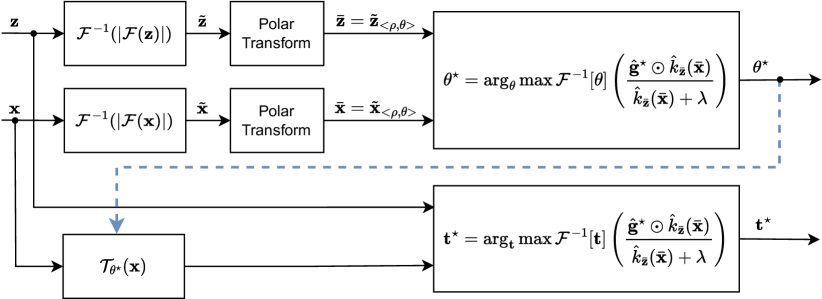
III-D Movement Decoupling

As shown in Fig. 2, to apply KCC in an efficient way, we decouple the rotation and translation movement, which is inspired by the properties of FFT and has been widely used in remote sensing [47]: translation in the space domain corresponds to phase shift in the frequency domain, while rotation in the space domain corresponds to the same rotation in the frequency domain. Suppose $\mathbf{x}$ is a translation and rotation transformation of $\mathbf{z}$, so we have $\mathbf{x}[i,j]=\mathbf{z}[i\cos\theta_{0}+j\sin\theta_{0}-i_{0},j\cos\theta_{0}-i\sin\theta_{0}-j_{0}]$, where $(i_{0},j_{0})$ is the translation and $\theta_{0}$ is the rotation angle, their FFT is $\hat{\mathbf{x}}[\zeta,\eta]=\hat{\mathbf{z}}[\zeta\cos\theta_{0}+\eta\sin\theta_{0},\eta\cos\theta_{0}-\zeta\sin\theta_{0}]e^{-2\pi(\zeta i_{0},\eta j_{0})}$. Therefore, the translation can be decoupled from rotation if we only take the FFT magnitude, i.e., $|\hat{\mathbf{x}}(\zeta,\eta)|=|\hat{\mathbf{x}}[\zeta\cos\theta_{0}+\eta\sin\theta_{0},\eta\cos\theta_{0}-\zeta\sin\theta_{0}]|$. In other words, there is only rotation transformation between two images $\tilde{\mathbf{x}}$ and $\tilde{\mathbf{z}}$:

$$\tilde{\mathbf{x}}=\mathcal{F}^{-1}(|\hat{\mathbf{x}}|),\quad\tilde{\mathbf{z}}=\mathcal{F}^{-1}(|\hat{\mathbf{z}}|),$$ (30)

where $\mathcal{F}^{-1}$ is the IFFT function. In this context, we can first estimate the rotation angle $\theta_{0}$ for new images (30) and then estimate translation $(i_{0},j_{0})$ for original rotated ($\theta_{0}$) images.

Recall that if a signal in one domain is real, then the signal in the other domain has to be symmetric, thus $\tilde{\mathbf{x}},\tilde{\mathbf{z}}$ are symmetric images, which will pose challenges for rotation estimation. Instead of resolving this ambiguity in rotation estimation, we estimate the translation of $\mathbf{z}$ for two rotation rectified images $\mathcal{T}_{\theta^{\star}}(\mathbf{x})$ and $\mathcal{T}_{\theta^{\star}+\pi}(\mathbf{x})$, where $\theta^{\star}$ is the estimated rotation angle, thus the final transform is the one with higher $P_{s}(\mathbf{x})$.

IV System Architecture

IV-A System Overview

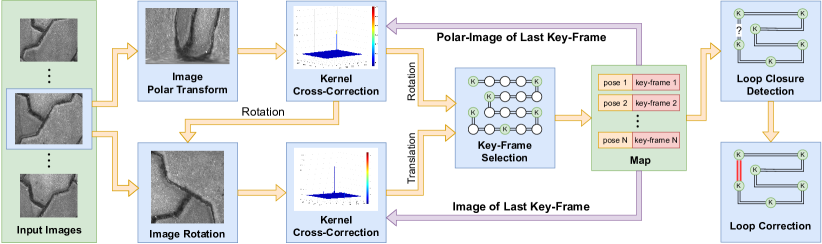
Using the methodology introduced in Section III, we developed a visual SLAM framework only using ground textures. The structure of this framework is depicted in Fig. 3. Our inputs comprise grayscale images taken by a camera mounted to face downward. The outputs are 3-DOF camera poses, specifically 2-DOF translations and rotation. The entire workflow is simple: The initial frame is designated as the first key-frame; Upon capturing a subsequent frame, the relative motion between the present and the key-frame is determined; Leveraging the estimated relative pose and its confidence, a new key-frame is chosen and integrated into the map; Subsequently, we identify its neighboring key-frames within the map, aiming to pinpoint a loop closure; If a loop closure is detected, we execute a pose graph optimization to minimize the drift error. We next present the details of each module, respectively.

IV-B Motion Estimation

IV-B1 Rotation

As discussed in Section III-D, the rotation and translation are decoupled and an initial rotation will be estimated first. To achieve this, each time a new image is captured, we generate a new image for it using (30). Then we remap the new image to polar space and call the result polar-image. With the help of Theorem 5, we can compute the transformation between the two generated images and then get the initial rotation angle $\theta^{\star}$. The corresponding confidence of the rotation estimation, $P_{s}^{r}$, can be computed through (24).

IV-B2 Translation

As a result of the ambiguity problem described in Section III-D, the real rotation $\theta_{I}$ could be $\theta^{\star}$ or $\theta^{\star}+\pi$. In the tracking stage, we have a prior assumption that the rotation between two nearby frames is not significant, therefore, the one with the smaller absolute value between $\theta^{\star}$ and $\theta^{\star}+\pi$ is selected as $\theta_{I}$. Then we rotate the current image by $\theta_{I}$ and compute the transformation between it and the last key-frame using Theorem 5. The estimated translation and the estimation confidence are denoted as $\mathbf{t_{I}}$ and $P_{s}^{t}$ respectively.

However, in the loop detection and map reuse stage, the prior assumption mentioned above is not valid. So to resolve the ambiguity, we rotate the current frame by $\theta^{\star}$ and $\theta^{\star}+\pi$, computing two translations $\mathbf{t_{1}^{\star}}$ and $\mathbf{t_{2}^{\star}}$ and their corresponding confidences $P_{s}^{t_{1}}$ and $P_{s}^{t_{2}}$ using Theorem 5 and (24), respectively. The final transform can be determined by

$$\left(\theta_{I},\mathbf{t_{I}},P_{s}^{t}\right)=\left\{\begin{array}[]{lcl}\left(\theta^{\star},\mathbf{t_{1}^{\star}},P_{s}^{t_{1}}\right)&\mbox{for}&\text{$P_{s}^{t_{1}}>=P_{s}^{t_{2}}$}\\ \left(\theta^{\star}+\pi,\mathbf{t_{2}^{\star}},P_{s}^{t_{2}}\right)&\mbox{for}&\text{$P_{s}^{t_{2}}>P_{s}^{t_{1}}$}.\end{array}\right.$$ (31)

IV-B3 Camera Pose

Note that $\theta_{I}$ and $\mathbf{t_{I}}$ are the rotation angle and 2D translation on the image plane, with the coordinate origin being at the image center. To get the relative camera pose, we first compute the rotation $\theta_{o}$ and the translation $\mathbf{t_{o}}$ with the principal point being the origin:

$$\theta_{o} =\theta_{I},$$ (32a)

$$\mathbf{t_{o}} =\left(\mathbf{I_{2\times 2}}-\mathbf{R}(\theta_{I})\right)\left[\begin{array}[]{c}W/2-c_{x}\\ H/2-c_{y}\end{array}\right]+\mathbf{t_{I}},$$ (32d)

where $W$, $H$ and $\left(c_{x},c_{y}\right)$ are the width, height, and principal point of the image, respectively. $\mathbf{I_{2\times 2}}$ denotes the 2D identity matrix. $\mathbf{R}(\theta_{I})$ is the rotation matrix generated by

$$\mathbf{R}(\theta_{I})=\left[\begin{array}[]{cc}\cos{\theta_{I}}&-\sin{\theta_{I}}\\ \sin{\theta_{I}}&\cos{\theta_{I}}\end{array}\right].$$ (33)

Then the relative camera pose can be obtained by

$$\left[\begin{array}[]{ccc}\theta_{c}&t_{c_{x}}&t_{c_{y}}\end{array}\right]^{\mathrm{T}}=\left[\begin{array}[]{ccc}\theta_{o}&\frac{h_{c}}{f_{x}}t_{o_{x}}&\frac{h_{c}}{f_{y}}t_{o_{y}}\end{array}\right]^{\mathrm{T}},$$ (34)

where $\theta_{c}$ and $\mathbf{t_{c}}$ are the camera rotation (the yaw angle) and translation, respectively, $f_{x}$ and $f_{y}$ are the focal lengths and $h_{c}$ is the height of the camera from the ground, which can be obtained from the camera extrinsic calibration.

IV-C Key-frame Selection

The accuracy of each motion estimation in Section IV-B is pixel-level, so to reduce the drift error, we select key-frames and only compute the relative pose between the current frame and the last key-frame. A frame will be selected as a key-frame if any one of the following conditions is satisfied:

• The distance to the last key-frame in the normalized image plane is larger than $\delta_{d}$;

• The angle with the last key-frame is larger than $\delta_{\theta}$;

• The confidence of rotation estimation falls within a predetermined range, i.e., $P_{s}^{r_{min}}<P_{s}^{r}<P_{s}^{r_{max}}$; and

• The confidence of translation estimation falls within a predetermined range, i.e., $P_{s}^{t_{min}}<P_{s}^{t}<P_{s}^{t_{max}}$,

where $\delta_{d}$, $\delta_{\theta}$, $P_{s}^{r_{min}}$, $P_{s}^{r_{max}}$, $P_{s}^{t_{min}}$ and $P_{s}^{t_{max}}$ are all preset thresholds. The first two conditions ensure sufficient overlap between the two frames. The last two conditions are to select fewer key-frames while ensuring the validity of the estimation.

IV-D Loop Detection

To correct the drift error, the loop closure should be detected if the robot goes back to a previously visited place. We maintain an online map that uses a hash table to store the indices, poses, FFT results, and polar images of key-frames. Once a new key-frame is inserted into the map, two kinds of verification are utilized to find a real loop.

IV-D1 Geometric Verification

We first retrieve all the key-frames within a distance of $d_{l}$ of the current key-frame as loop candidates. To avoid the false loop pair with neighboring key-frames, candidates with a travel distance less than $\delta_{d}^{l}$ or an index difference less than $\delta_{N}^{l}$ from the current frame will be removed. Generally speaking, geometric verification can rapidly filter out the majority of outliers.

IV-D2 Correction Verification

For each remaining key-frame, the relative pose to the current key-frame will be computed. The candidate with the highest confidence is taken as the best loop candidate, and if its rotation estimation confidence is higher than $P_{s}^{r_{\mathrm{min}}}$ and translation estimation confidence is higher than $P_{s}^{t_{\mathrm{min}}}$, it will be considered as a valid loop closure.

Once a new valid loop closure is detected, a pose graph of key-frames is then constructed. It contains two kinds of edges: the odometry edges, which connect two adjacent key-frames, and the loop edges, which connect the loop closure pairs. The graph can be optimized using the Levernberg-Marquardt algorithm [48]. The poses of key-frames in the map will be updated once the optimization is finished.

Algorithm 1 Map Reuse

0:  $\mathbf{x}$: the current image; $\left\{\mathbf{x_{i}^{k}},i<N\right\}$: the candidates; $\left(P_{s}^{r_{min}},P_{s}^{t_{min}}\right)$: confidence thresholds;

0:  $\left(\theta,\mathbf{t}\right)$: the current pose, $P_{s}$: the confidence;

1:  Initialization: $i=0$ and $P_{s}=0$;

2:  for $i<N$ do

3:     $i\leftarrow i+1$

4:     $\Delta{\theta_{i}},P_{s}^{r_{i}}=\mathrm{RotationEstimation}(\mathbf{x_{i}^{k}},\mathbf{x})$

5:     if $P_{s}^{r_{i}}>P_{s}^{r_{min}}$ then

6:        $\mathbf{\Delta t_{i}},P_{s}^{t_{i}}=\mathrm{TranslationEstimation}(\mathbf{x_{i}^{k}},\mathbf{x})$

7:        if $P_{s}^{t_{i}}>P_{s}^{t_{min}}$ and $P_{s}<(P_{s}^{r_{i}}+P_{s}^{t_{i}})$ then

8:           $P_{s}\leftarrow P_{s}^{r_{i}}+P_{s}^{t_{i}}$

9:           $\theta\leftarrow\theta_{i}^{k}+\Delta{\theta_{i}}$

10:           $\mathbf{t}\leftarrow\mathbf{t_{i}^{k}}+\mathbf{R}(\theta_{i}^{k})\mathbf{\Delta t_{i}}$

11:        end if

12:     end if

13:  end for

IV-E Map Reuse

In real applications like warehouse logistics, a prior map is usually built in advance and then other robots can use this map for drift-free localization. In this section, we demonstrate how to save and reuse a prior map. Different from current methods that are based on various features, descriptors and Bag of Words [27], our map reuse module utilizes our KCC to compute the similarity between two frames. Therefore, unlike other visual maps that must store point clouds, descriptors, and the observation relationship, the map used in the proposed system is cleaner and simpler. We only store the poses, the FFT results, and the polar-images of key-frames. Note that the poses of key-frames can be generated not only by the system described earlier but also by other systems, e.g., other visual or LiDAR SLAM systems, ultra-wideband (UWB) or even high-precision measurement devices.

When deploying the built map in the warehouse, we take the local localization strategy rather than the global localization for higher accuracy and efficiency. For each query image, we use a prior pose to retrieve all the neighboring key-frames within a distance of $d_{mr}$ as candidates. The threshold $d_{mr}$ depends on the covariance of the prior pose. Then we use Algorithm 1 to compute the current pose and the corresponding confidence $P_{s}$. The estimation is considered valid if $P_{s}>0$.

V Experiments

The remainder of this section is organized as follows. In Section V-A, we introduce the baselines and datasets used in the following experiments. Our field-collected dataset, the GeoTracking dataset, is also introduced. We then evaluate the performance on data association, visual odometry, loop detection, map reuse, and real-world demo in Section V-B, V-C, V-D, V-E, and V-F, respectively. The ablation study on the effects of the kernel method and analysis on system efficiency are presented in Section V-G and V-H, respectively.

Figure 4: Example ground texture images in our dataset. We collect 10 kinds of ground textures, including 6 kinds of outdoor textures and 4 kinds of indoor textures, which are marked in blue and red respectively.

V-A New Datasets and Baselines

V-A1 Datasets

To our current understanding, there exist only two publicly accessible ground texture datasets: Micro-GPS [8] and the HD Ground dataset [33]. Notably, both these datasets primarily target the evaluation of re-localization systems that utilize prior maps. This design inclination yields two specific attributes that render them less effective for the assessment of VO and SLAM systems: (1) Limited Overlap: These datasets aim for wide area coverage with fewer images, emphasizing visual aliasing effects [33]. In pursuit of this objective, they re-sample the original image sequences, producing new sequences. However, the sampling strategy leads to minimal overlap between successive frames, making them not ideal for evaluating VO and SLAM systems. (2) Ground Truth Accuracy Concerns: The datasets rely on image stitching to establish their ground truths, as opposed to leveraging precise pose measurement instruments. This means that their accuracy is largely dependent on the feature detection and matching in the image-stitching algorithm. However, we found that our KCC-based image matching can even produce higher accuracy than feature-based matching (will be detailed in Section V-B). This suggests that those datasets might not be sufficiently robust for evaluating accuracy. Consequently, we exclude the Micro-GPS dataset and solely rely on the HD Ground dataset to evaluate data association, map reuse, and the success tracking rate.

To solve this problem and facilitate a comprehensive evaluation of VO and SLAM systems, we introduce the GeoTracking dataset. We utilized a modified Weston SCOUT Robot as our primary data collection platform. This robot is outfitted with an IDS uEye monocular camera, strategically positioned at its base facing downward, maintaining a height of $0.1\mathrm{m}$ above the terrain. To achieve consistent illumination, an array of LED lights encircles the camera, following the configuration of most warehouse robots. For accurate ground truth measurements, we affixed a prism atop the robot, which is continuously monitored by a Leica Nova MS60 MultiStation laser tracker.

TABLE I: A comparison between our dataset and the HD Ground dataset.

Datasets	HD Ground [33]	GeoTracking (Ours)
Images	201428	131300
Images Per Meter	14.98	242.28
Avg Overlap	35.21%	93.69%
Textures Types	11	10
Textures with Long Sequence	7	10
Avg Sequence Length ( m )	11.18	30.11
Max Sequence Length ( m )	55.09	55.47
Ground Truth	Image Stitching	Leica Total Station

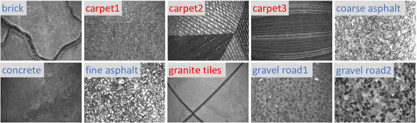
As depicted in Fig. 4, our GeoTracking dataset encompasses 10 prevalent ground textures, segmented into 6 outdoor and 4 indoor textures. A comparative analysis against the HD Ground dataset is presented in Table I. Herein, the overlap between successive frames is defined by their intersection over union (IOU). The metric “Textures with Long Sequence” signifies the count of texture categories with sequences extending beyond $15\mathrm{m}$. The “Max Sequence Length” denotes the single longest sequence’s span. A notable observation is that the average overlap between adjoining frames in our dataset is about 2.6 times greater than the HD Ground dataset, making our dataset ideal for evaluating the frame-by-frame tracking performance of different SLAM systems. Moreover, our dataset leads in the average sequence length and the number of textures featuring extended sequences, which provides a more effective assessment for SLAM systems over long distances.

Figure 5: The comparison of data association of ORB, SIFT, and KCC on the HD Ground dataset. The numbers of features and matching inliers are given. For the KCC, the correction results are projected to three coordinate axes and represent the estimation of the 3-DOF movement. The vertical axis is the confidence of estimated movement on the horizontal axis. The higher the value of the peak relative to other positions, the greater the confidence of motion estimation.

TABLE II: Translational error (RMSE) without loop closing on the GeoTracking dataset (unit: m). $\times$ refers to tracking lost.

Sequence	Length ( m )	BRISK-VO	SURF-VO	SIFT-VO	GT-SLAM	SVO	ORB-SLAM3	Ours
Brick_seq1	14.06	0.5831	0.6338	0.5449	0.1524	0.1498	0.1255	0.1624
Brick_seq2	24.55	0.2486	0.5028	0.4795	1.2155	0.3369	0.2272	0.2131
Carpet1_seq1	43.23	3.4206	3.9871	3.1069	5.9145	6.3791	$\times$	1.1072
Carpet1_seq2	38.37	1.9755	2.2477	1.8252	0.3773	1.1517	0.1450	0.4228
Carpet2_seq1	41.47	1.7463	1.7161	1.4816	0.7033	$\times$	$\times$	0.2893
Carpet3_seq1	16.64	$\times$	0.3484	0.3492	1.6733	0.2647	$\times$	0.1737
Carpet3_seq2	19.01	$\times$	0.5366	0.5970	0.7360	0.4485	$\times$	0.2520
Carpet3_seq3	45.04	$\times$	0.8639	3.2845	5.2281	$\times$	$\times$	0.3758
Coarse_asphalt_seq1	15.55	$\times$	0.6909	0.7462	0.2172	0.0820	0.1201	0.1634
Concrete_seq1	23.40	$\times$	$\times$	1.0102	2.0773	0.7759	$\times$	0.3605
Concrete_seq2	23.53	$\times$	$\times$	$\times$	0.6635	0.7143	$\times$	0.2621
Fine_asphalt_seq1	22.18	1.2376	1.1943	1.1109	1.0329	0.2410	0.2662	0.1599
Fine_asphalt_seq2	55.47	2.2659	2.3832	2.2640	2.1359	$\times$	$\times$	0.1713
Granite_tiles_seq1	27.16	$\times$	$\times$	$\times$	0.6036	0.1803	$\times$	0.4693
Granite_tiles_seq2	40.66	$\times$	$\times$	0.6867	0.8662	0.2867	$\times$	0.5178
Gravel_road1_seq1	17.52	$\times$	0.9282	1.0861	0.6887	0.1665	0.2179	0.1663
Gravel_road2_seq1	46.11	1.5206	1.5650	1.4908	0.8546	0.4140	0.4224	0.3391

V-A2 Baselines

We compare our systems with two kinds of baselines: (1) Ground-texture-based systems. Such systems estimate the 2D rotation and translation from feature extraction and matching. The Ground-Texture-SLAM (GT-SLAM) [25] maintains a good balance between efficiency and performance. It uses ORB [49] features in both front-end and loop closure detection. Since feature type plays an important role in ground-texture-based SLAM systems, we implemented the visual odometry with SIFT [23], SURF [21], and BRISK [50] to investigate the performance of other features, and name them SIFT-VO, SURF-VO, and BRISK-VO, respectively. (2) Monocular visual SLAM systems. To investigate the performance of other widely-used visual SLAM systems, we compare with feature-based method ORB-SLAM3 [51] and direct method SVO [52]. Other ground-texture-based localization systems [6, 5, 9, 7, 29] are not included because their source code is unavailable.

Figure 6: Estimated trajectories by our system (NI-SLAM) and GT-SLAM on 4 sequences of the GeoTracking dataset. The trajectories have been aligned with ground truth by evo [53].

V-B Data Association

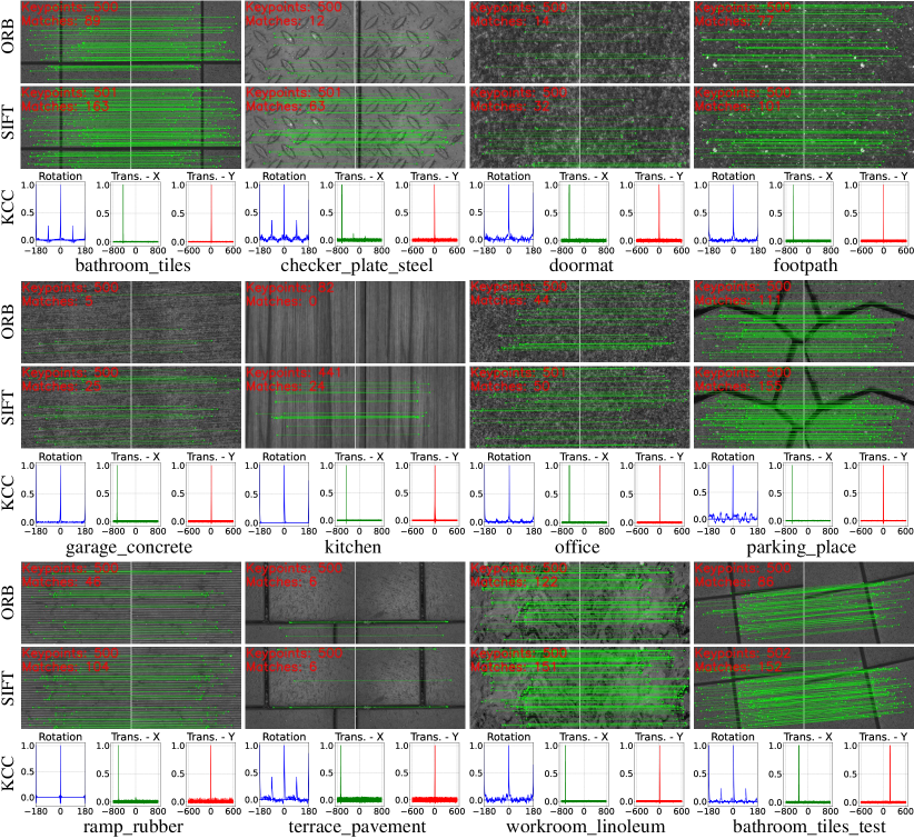
To benchmark the performance in low-overlap and different textures, we first evaluate the performance on data association using the HD Ground dataset. The matching performance of the ORB and SIFT features and our KCC are shown in Fig. 5. Since KCC operates as an image-matching technique, its estimation is graphically represented with the normalized confidence on the vertical axis, while the horizontal axis details the corresponding movements in rotation and translation. It can be seen that KCC consistently demonstrates accuracy and stability across diverse ground textures. This is evident from the distinctly pronounced peaks that tower significantly over other positions. However, the performance of feature-based methods fluctuates. They show commendable results on textures enriched with unique corners, such as in the sequence of “bathroom_tiles”, “footpath”, “parking_place”, and “workroom_linoleum”; while struggling to detect a sufficient number of matches in the sequence of “checker_plate_steel”, “doormat”, “garage_concrete”, “office”, and “terrace_pavement”. The situation further deteriorates with the “kitchen” texture, where they fail to even detect an adequate number of features.

V-C Visual Odometry

To compare the performance of frame-by-frame tracking and pose estimation among different SLAM systems, we conduct the odometry experiment where the loop detection and relocalization modules are removed from all the methods.

V-C1 Accuracy on the GeoTracking Dataset

The efficacy of various systems, when benchmarked against the GeoTracking dataset, is evaluated using the Root Mean Square Error (RMSE) of translation and detailed in Table II. Given that only positional ground truth data is accessible, a comparative analysis of rotational errors is omitted. The top-performing results are distinctly highlighted and underlined in order. On an overarching scale, our system’s resilience and precision stand unparalleled. It maintains consistent tracking across all sequences, securing minimal translational error in 12 out of the 17 sequences, indicating its best robustness over all other algorithms. We notice that on some sequences such as “Brick”, “Coarse_asphalt”, “Granite_tiles”, and “Gravel_road”, SVO and ORB-SLAM3 achieved slightly better performance than NI-SLAM. This is because images of these sequences have more distinctive corners or edges, which are easy to track by feature-based methods. However, their dependence on prominent features or edges results in poor performance on the ground with minimal texture, leading to frequent tracking lost in scenarios like “Concrete”, “Carpet”, “Fine_asphalt”, and “Granite_tiles”. In contrast, our NI-SLAM consistently delivers stable and dependable results across all sequences.

Figure 7: Comparison on the “Gravel_road2_seq1” of the GeoTracking dataset. The vertical axis is the proportion of pose errors that are less than the given alignment error threshold on the horizontal axis.

TABLE III: Proportion of successful runs (%) on the HD Ground dataset. The best results are highlighted.

Texture	Sequences	BRISK-VO	SURF-VO	SIFT-VO	GT-SLAM	GT-SLAM${}^{\text{w/o cvm}}$	Ours
bathroom_tiles	31	38.71	100	100	61.29	61.29	96.77
checker_plate_steel	12	8.33	25.00	41.67	0	0	75.00
doormat	25	40.00	64.00	64.00	4.00	4.00	76.00
footpath	18	100	100	100	88.89	88.89	94.44
garage_concrete	92	2.17	4.35	84.78	0	0	93.48
kitchen	25	0	24.00	24.00	64.00	4.00	100
office	24	87.50	75.00	100	83.33	79.17	100
parking_place	25	96.00	88.00	100	84.00	68.00	100
ramp_rubber	43	79.07	95.35	100	0	0	100
terrace_pavement	49	0	0	0	0	0	71.43
workroom_linoleum	60	100	100	100	30.00	30.00	76.67

• The results of SVO and ORB-SLAM3 are not listed as they fail to initialize on most sequences due to the limited overlap between images.

Robustness Analysis

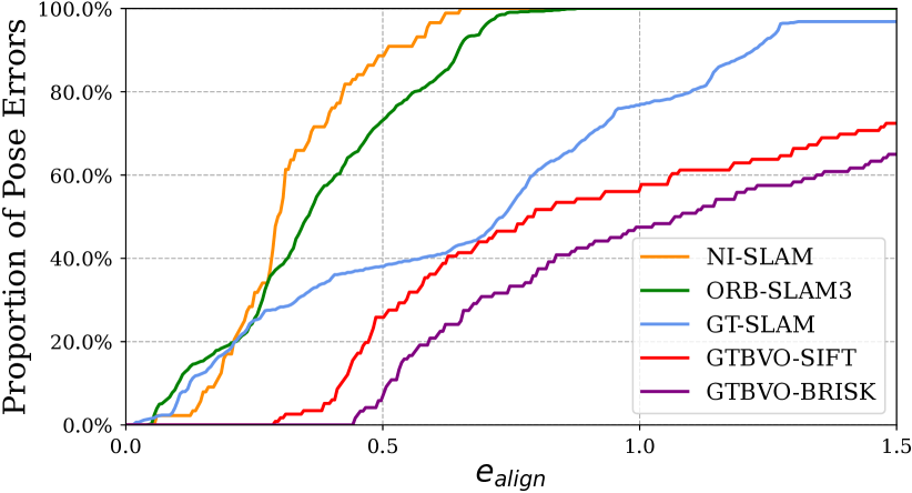
We show the trajectories produced by our system and GT-SLAM on 4 sequences in Fig. 6. It can be seen that the drift errors of our system are much smaller than GT-SLAM. A comparison of error distributions on the “Gravel_road2_seq1” is shown in Fig. 7. The vertical axis is the proportion of pose errors that are less than the given threshold on the horizontal axis. Given a certain error threshold, it is better when the proportion is higher. It can be seen that the number of poses with a pose error less than $0.3\mathrm{m}$ is roughly the same for ORB-SLAM3, GT-SLAM, and our system. However, more than 90% of the pose errors of our NI-SLAM are less than $0.5\mathrm{m}$, which outperforms all other methods.

Additionally, we find that although GT-SLAM and ORB-SLAM3 use the same ORB feature, there is a significant performance difference between these two systems. GT-SLAM is more robust while ORB-SLAM3 is more accurate. This may be due to the different feature tracking and optimization methods. ORB-SLAM3 predicts the camera pose with a constant velocity model and then projects 3D points onto the image to match the features. We find it is more efficient but less robust than the FLANN-based method [26] used in GT-SLAM when dealing with ground texture images. In the optimization stage, GT-SLAM only constructs a simple pose graph, while ORB-SLAM3 optimizes a co-visibility graph that contains both poses and map points, which may result in the accuracy difference between these two systems.

V-C2 Performance on the HD Ground Dataset

We find the feature-based methods (GT-SLAM, SVO and ORB-SLAM3) can easily lose track in the HD Ground dataset due to the limited number of detected features; and different methods usually experience tracking lost on different textures. This makes it difficult to compare these methods using the RMSE metric. Therefore, we use the success rate $S_{m}=n_{s}/N_{s}$ instead of tracking error to evaluate their performance, where $N_{s}$ and $n_{s}$ are the number of sub-sequences and successful runs, respectively. A successful run refers to the translational and rotation errors are less than $0.05\mathrm{m}$ and $10^{\circ}$, respectively.

TABLE IV: Translational error (RMSE) with loop detection and correction (unit: m). The best results are highlighted.

Sequence	GT-SLAM${}^{\text{LOOP}}$	NI-SLAM	NI-SLAM${}^{\text{LOOP}}$
Carpet1_seq2	0.4554	0.4228	0.2953
Carpet2_seq1	0.3931	0.2893	0.2584
Carpet3_seq2	0.4796	0.2520	0.2505
Fine_asphalt_seq2	1.2263	0.1713	0.1311
average	0.6386	0.2839	0.2293

The results are presented in Table III. As there is not too much overlap between adjacent images, SVO and ORB-SLAM3 fail to initialize their systems on most sequences. Therefore, their results are not listed in Table III. GT-SLAM${}^{\text{w/o cvm}}$ refers to GT-SLAM without the constant velocity model when losing track. It can be seen that our NI-SLAM achieves the best results on 8 out of the 11 textures, and it is the only system that achieves success rates of over 70% on all the textures, which proves the robustness of the proposed system.

The feature-based methods perform well on the textures with rich distinctive corners such as in sequences of “footpath” and “workroom_linoleum”, but experience a lot of tracking failures on the textures with few corners like “kitchen” or many repetitive features like “terrace_pavement” and “checker_plate_steel”. The VO experiment results on the HD Ground dataset are consistent with the data association experiment results in Section V-B. The performance difference between GT-SLAM and GT-SLAM${}^{\text{w/o cvm}}$ originates the fact that GT-SLAM uses the constant velocity model for pose estimation when tracking is lost, which allows it to yield successful runs even if it loses many tracks on the straight sequences.

Figure 8: Trajectories estimated by NI-SLAM, NI-SLAM${}^{\text{LOOP}}$ and the ground truth on the Fine_asphalt_seq2 sequence of the GeoTracking dataset.

Figure 9: The pose errors (RMSE) of NI-SLAM and NI-SLAM${}^{\text{LOOP}}$ on the Fine_asphalt_seq2 sequence of the GeoTracking dataset.

V-D Loop Detection

Given the absence of loop closures in the HD Ground dataset, our focus is exclusively on sequences within the GeoTracking dataset that exhibit pronounced loop closures. In this comparative analysis, our proposed system equipped with loop correction is denoted as NI-SLAM${}^{\text{LOOP}}$, while the variant of GT-SLAM with loop correction is represented as GT-SLAM${}^{\text{LOOP}}$. The outcomes of this comparison are tabulated in Table IV. Notably, ORB-SLAM3 is excluded from the results due to its prevalent tracking failures across most sequences. The introduced loop detection and correction techniques culminate in a marked reduction of the translation error by 30.2%, 10.7%, 0.6%, and 23.5% across the four distinct sequences. Impressively, NI-SLAM${}^{\text{LOOP}}$ consistently surpasses GT-SLAM${}^{\text{LOOP}}$ across all four sequences. Besides, compared with the results in Table III, we find adding loop detection has increased the error of GT-SLAM${}^{\text{LOOP}}$ on the sequence “Carpet1_seq2”. It is because GT-SLAM${}^{\text{LOOP}}$ detected a false loop closure on this sequence due to similar patterns. The incorrect loop detection did not appear in NI-SLAM, which indicates the robustness of our method. It’s also important to highlight that our NI-SLAM system, even without loop closure correction, performed notably better than GT-SLAM${}^{\text{LOOP}}$, further demonstrating the reliability of NI-SLAM.

Robustness Analysis

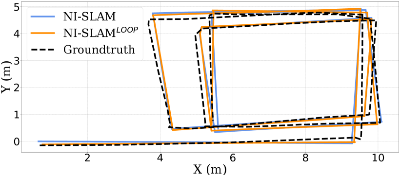
Fig. 8 and Fig. 9 show a comparison of NI-SLAM and NI-SLAM${}^{\text{LOOP}}$ on the “Fine_asphalt_seq2” sequence. This sequence has a total length of $55\mathrm{m}$ and it is the longest sequence in the GeoTracking dataset. Its trajectory creates three loops, resulting in loop closures. It is seen that the trajectory of NI-SLAM${}^{\text{LOOP}}$ is closer to the ground truth than the trajectory of NI-SLAM. The pose errors are significantly decreased after the loop correction. Note that the other methods such as SVO and ORB-SLAM3 constantly lose track in this sequence, which further indicates the robustness of our method.

TABLE V: Recall of map reuse(%). The best results are highlighted.

Texture	GT-SLAM	Ours	Improvement
bathroom_tiles	93.92	98.25	+ 4.33
checker_plate_steel	85.33	99.13	+ 13.80
doormat	48.70	88.26	+ 39.56
footpath	66.10	93.39	+ 27.29
garage_concrete	56.16	99.93	+ 43.77
kitchen	2.08	91.22	+ 89.14
office	88.11	98.92	+ 10.81
parking_place	87.37	98.57	+ 11.20
ramp_rubber	21.60	94.18	+ 72.58
terrace_pavement	61.51	92.83	+ 31.32
workroom_linoleum	90.85	99.79	+ 8.94
average	63.79	95.86	+ 32.07

V-E Map Reuse

Map reuse can provide drift-free localization with a prior map and thus it is essential for the real application. To compare with the feature-based methods, we again select GT-SLAM, which is the state-of-the-art feature-based system, as the baseline. The HD Ground dataset is utilized because it records both mapping data and test data in the same areas. The mapping data is treated as a database, and the images in the test data are used to query the database for similar images. The pose of the queried image is determined by calculating the relative pose with the database image. As described in Section IV-E, a prior pose of the query images is provided for a real-time and robust re-localization, which is very common in real applications.

We randomly create the prior pose within a range of half a meter from the ground truth position of the query image and provide it to both GT-SLAM and our system. We refer to localization as successful if the pose estimation for a query image has a translation error of less than 2mm (approximately 20 pixels) and an angular error of less than $1.15^{\circ}$ (around 0.02 rad). The benchmark-setting here is notably more rigorous compared to those in Section V-C given the drift-free nature of pose estimation in this context. We introduce the recall rate as a metric, which is the ratio of the number of successful localizations against the cumulative number of test images. The results of the experiment are tabulated in Table V. It is evident that our system consistently outperforms GT-SLAM across diverse textures. The recall rates registered for NI-SLAM consistently exceed 88%, marking an average enhancement of 32.07% over GT-SLAM. Remarkably, for textures characterized by sparse corners, such as the “kitchen” texture, the boost in performance nears a significant 90%. This underscores the resilience and robustness inherent to our system.

TABLE VI: The RMSE (cm) comparison in the ablation study. The best results are highlighted. $\times$ refers to tracking lost

Sequence	Full Sequence		Translation Parts Only1
	w/o k.	Ours	w/o k.	Ours	Reducing
Brick_seq1	$\times$	16.24	2.42	1.77	- 0.64
Brick_seq2	$\times$	21.31	3.04	3.33	+ 0.29
Carpet1_seq1	$\times$	110.72	$\times$	8.89	-
Carpet1_seq2	$\times$	42.28	7.00	6.80	- 0.20
Carpet2_seq1	$\times$	28.93	4.10	3.67	- 0.43
Carpet3_seq1	$\times$	17.37	$\times$	3.17	-
Carpet3_seq2	$\times$	25.20	3.00	3.76	+ 0.76
Carpet3_seq3	$\times$	37.58	4.07	4.14	+ 0.07
Coarse_asphalt_seq1	$\times$	16.34	3.52	2.63	- 0.89
Concrete_seq1	$\times$	36.05	20.94	3.23	- 17.71
Concrete_seq2	$\times$	26.21	3.93	3.81	- 0.12
Fine_asphalt_seq1	$\times$	15.59	2.67	2.79	+ 0.12
Fine_asphalt_seq2	$\times$	17.13	2.44	3.82	+ 1.38
Granite_tiles_seq1	$\times$	46.93	$\times$	3.22	-
Granite_tiles_seq2	$\times$	51.78	3.79	1.35	- 2.44
Gravel_road1_seq1	$\times$	16.63	11.11	2.58	- 8.53
Gravel_road2_seq1	$\times$	33.91	$\times$	3.67	-
average	$\times$	31.75	5.54	3.69	- 1.85

• As the system without kernel (w/o k.) fails to estimate the rotation, we use the translational parts of the GeoTracking dataset for comparison.

Figure 10: A live mapping demo of NI-SLAM without (left) and with (right) loop correction. The robot moves in a rectangular path (the green line) with the starting and ending being at the same location (the red square). The drift error of our VO module is only 0.2% of the trajectory, which is significantly lower than other SOTA systems (about 1%). The drift error causes the blurring in the stitched map (left), and it is eliminated by our loop correction (right).

V-F Live Mapping Demo

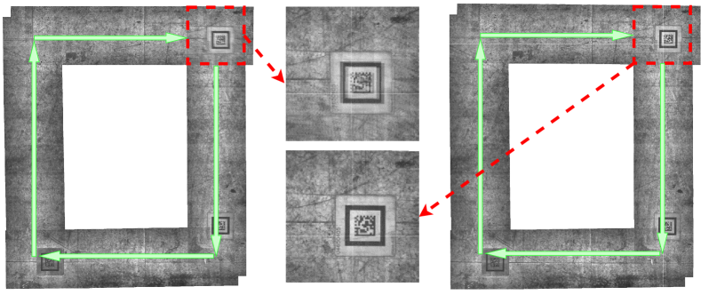
We showcase a real-time mapping demonstration with loop detection and correction. This data is gathered in a warehouse setting by an Automated Guided Vehicle (AGV), as depicted in Fig. 1. The robot is fitted with a downward-facing camera, initially intended for localization via QR code scanning (only for ground truth). We maneuvered the robot along a rectangular trajectory (highlighted by the green line) to initiate and stop at the identical location (indicated by the red square), effectively creating a loop. Images from this path are then composited using the pose estimates produced by NI-SLAM, both without (on the left) and with (on the right) loop correction in Fig. 10. Due to the drift error, the stitched map without loop correction exhibits noticeable blurring, which is eliminated on the right. This clarity underscores the effective elimination of drift errors and the precise pose corrections. Note that we have also tested NI-SLAM with this AGV in a real industrial operating area of more than 10,000 □ m . It shows consistent robustness and accuracy. However, due to a lack of ground truth, we are not able to show their quantitative performance.

V-G Ablation Study

The kernel method proposed in Section III is essential for rotation estimation and the motion estimation can easily fail after removing the kernel function from KCC. To quantitatively evaluate this, we first evaluate the system without kernel function and find it lost track in all sequences of the GeoTracking dataset. Next, to verify the effectiveness of the proposed kernel method on the translation estimation, we extract the translational parts of the GeoTracking dataset and use them to compare our NI-SLAM with the system without kernel function. Table VI shows the result, where “w/o k.” represents NI-SLAM without the kernel function. It can be seen that adding the kernel function reduces the translation errors on 12 out of 17 sequences. The average error decreases by about 33%. The experiment result indicates that the proposed kernel method has brought significant improvements: First, it empowers the system’s ability to estimate the rotation movements; Second, it increases the accuracy of the system’s translation estimation.

Figure 11: Efficiency analysis for different systems on the GeoTracking dataset. The vertical axis is the average runtime of each frame. The horizontal axes are the CPU usage (left) and average RMSE (right), respectively.

V-H Efficiency Analysis

This section presents the efficiency analysis of our NI-SLAM. The evaluation is performed on a computer with an Intel i9-13900 CPU. We use the GeoTracking dataset and the image resolution is $640\times 480$. We first compare the running speed, computing resource consumption, and the accuracy of different systems. The metrics are per-frame runtime, CPU usage, and average RMSE. For the sequence with tracking failures, we set the error to $10\mathrm{m}$ when computing the average RMSE. The results are shown in Fig. 11. Overall, NI-SLAM achieves the best accuracy, consumes fewer computational resources, and can run in real-time. GT-SLAM ranks second in accuracy, but it lags considerably behind our NI-SLAM. It runs a little faster but consumes more resources than ours. ORB-SLAM3 and BRISK-VO have a similar level of efficiency to our system. However, they experience many tracking failures and thus have large average errors. SVO is the most efficient system, but its accuracy is also significantly lower than other systems.

We also list the runtime of each module of our system in Table VII. The front-end processing for one frame takes 32.43 m s  and the back-end modules take 53.98 m s . Note that the back-end modules (loop detection and loop correction) only perform on key-frames, so the runtime difference between NI-SLAM with and without loop correction is not significant.

TABLE VII: Runtime analysis of each module in NI-SLAM.

	Module	Average Runtime ( m s )
Front-end	Undistortion	0.35
	FFT	1.56
	Polar-Image	4.34
	Rotation	9.90
	Translation	13.99
	Keyframe Selection	0.01
	Others	2.28
	Total	32.43
Back-end	Loop Detection	37.87
	Loop Correction	16.11

VI Discussion

We presented a novel visual SLAM system, NI-SLAM, for the warehouse robot with a downward-facing camera using ground textures, which includes non-iterative visual odometry, loop closure detection, and map reuse. Our system can provide robust localization in dynamic and large-scale environments using only a monocular camera. Specifically, a kernel cross-correlator was introduced for image-level registration, which makes our system more robust and reliable when dealing with ground images with few features or repetitive patterns than feature-based methods. We showcased the proficiency and efficacy of NI-SLAM, highlighting its advantages over leading ground-texture-based localization systems and visual SLAM systems. To benefit the entire community, we also released the source code and the first ground-texture-based dataset, GeoTracking with accurate pose ground truth.

Despite its excellent performance for warehouse robots using ground textures, the proposed system still has two limitations. First, as mainly designed for warehouse robots, it estimates the 3-DOF transformation instead of the 6-DOF transformation. Therefore, our system can not be deployed on the robot with 6-DOF movements such as the unmanned aerial vehicle (UAV). Second, the proposed map reuse method needs a prior pose. It requires an initial rough position when the robot boots up.

VII Acknowledgment

The authors would like to thank Dr. Yuan Shenghai and Geekplus Technology Co., Ltd. for collecting the data.

Appendix A Cross-Correlation Theorem

In signal processing, cross-correlation is a similarity measurement of two signals as a function of the displacement of one relative to the other, which is also known as a sliding inner-product[54]. Denote two real finite discrete signals as $\mathbf{x},\mathbf{h}\in\mathbb{R}^{m}$, the circular cross-correlation $\otimes$ can be defined as

$$({\mathbf{x}}\otimes\mathbf{h})[m]=\sum_{i=0}^{n-1}\mathbf{x}[i]\mathbf{h}[(m+i)_{\bmod n}]=\mathbf{x}^{T}\mathbf{h}_{(m)},$$ (35)

where the bracket $\cdot[m]$ is to access the $m^{\text{th}}$ element of a vector, $\cdot_{\bmod n}$ is the modular arithmetic operation and the subscript $\cdot_{(m)}$ denotes the left circular rotation of a vector by $m$ elements. The definition of circular cross-correlation (35) is useful for understanding its behaviors, while it is often calculated using discrete Fourier transform (DFT) based on the circular cross-correlation theorem, which is also known as cross-correlation theorem for short. We denote $\hat{\mathbf{x}}=\mathcal{F}(x)$ as the DFT output.

Lemma 6 (Cross-Correlation Theorem [44]).

The DFT of the circular cross-correlation (35) on two finite discrete signals is equivalent to element-wise conjugate multiplication of the DFT of individual signals, i.e.,

$$\mathcal{F}(\mathbf{x}\otimes\mathbf{h})=\hat{\mathbf{x}}\odot\hat{\mathbf{h}}^{*},$$ (36)

where the superscript ${\cdot}^{*}$ denotes the complex conjugate and $\odot$ is the element-wise multiplication.

Theorem 6 indicates that a circular cross-correlation of two finite signals can be obtained via the element-wise product of their individual DFT. This is crucial for many applications, in which the DFT is often calculated by efficient fast Fourier transform (FFT). For example, Rader’s algorithm [55] is only of complexity $\mathcal{O}(n\log n)$, where $n$ is the length of the signal.

References

- [1] C. Cadena, L. Carlone, H. Carrillo, Y. Latif, D. Scaramuzza, J. Neira, I. Reid, and J. J. Leonard, “Past, present, and future of simultaneous localization and mapping: Toward the robust-perception age,” IEEE Transactions on robotics, vol. 32, no. 6, pp. 1309–1332, 2016.
- [2] K. Xu, Y. Hao, S. Yuan, C. Wang, and L. Xie, “AirVO: An illumination-robust point-line visual odometry,” in IEEE/RSJ International Conference on Intelligent Robots and Systems (IROS), 2023. [Online]. Available: https://arxiv.org/pdf/2212.07595.pdf
- [3] Y. Qiu, C. Wang, W. Wang, M. Henein, and S. Scherer, “AirDOS: Dynamic slam benefits from articulated objects,” in International Conference on Robotics and Automation (ICRA), 2022. [Online]. Available: https://arxiv.org/pdf/2109.09903
- [4] S. Xu, Y. Dong, H. Wang, S. Wang, Y. Zhang, and B. He, “Bifocal-binocular visual slam system for repetitive large-scale environments,” IEEE Transactions on Instrumentation and Measurement, vol. 71, pp. 1–15, 2022.
- [5] K. Kozak and M. Alban, “Ranger: A ground-facing camera-based localization system for ground vehicles,” in 2016 IEEE/ION Position, Location and Navigation Symposium (PLANS). IEEE, 2016, pp. 170–178.
- [6] X. Chen, A. S. Vempati, and P. Beardsley, “Streetmap-mapping and localization on ground planes using a downward facing camera,” in 2018 IEEE/RSJ International Conference on Intelligent Robots and Systems (IROS). IEEE, 2018, pp. 1672–1679.
- [7] S. Nakashima, T. Morio, and S. Mu, “Akaze-based visual odometry from floor images supported by acceleration models,” IEEE Access, vol. 7, pp. 31 103–31 109, 2019.
- [8] L. Zhang, A. Finkelstein, and S. Rusinkiewicz, “High-precision localization using ground texture,” in 2019 International Conference on Robotics and Automation (ICRA). IEEE, 2019, pp. 6381–6387.
- [9] J. F. Schmid, S. F. Simon, and R. Mester, “Ground texture based localization using compact binary descriptors,” in 2020 IEEE International Conference on Robotics and Automation (ICRA). IEEE, 2020, pp. 1315–1321.
- [10] M. Bloesch, J. Czarnowski, R. Clark, S. Leutenegger, and A. J. Davison, “Codeslam—learning a compact, optimisable representation for dense visual slam,” in Proceedings of the IEEE conference on computer vision and pattern recognition, 2018, pp. 2560–2568.
- [11] S. Zhi, M. Bloesch, S. Leutenegger, and A. J. Davison, “Scenecode: Monocular dense semantic reconstruction using learned encoded scene representations,” in Proceedings of the IEEE/CVF Conference on Computer Vision and Pattern Recognition, 2019, pp. 11 776–11 785.
- [12] S. Shen, Y. Cai, W. Wang, and S. Scherer, “Dytanvo: Joint refinement of visual odometry and motion segmentation in dynamic environments,” in 2023 IEEE International Conference on Robotics and Automation (ICRA). IEEE, 2023, pp. 4048–4055.
- [13] M. Tang and J. Feng, “Multi-kernel Correlation Filter for Visual Tracking,” in IEEE International Conference on Computer Vision. IEEE, 2015, pp. 3038–3046.
- [14] M. Danelljan, F. S. Khan, G. Hager, and M. Felsberg, “Discriminative Scale Space Tracking,” IEEE Transactions on Pattern Analysis and Machine Intelligence, pp. 1–1, 2017.
- [15] C. Wang, J. Yuan, and L. Xie, “Non-iterative SLAM,” in International Conference on Advanced Robotics (ICAR). IEEE, 2017, pp. 83–90.
- [16] C. Wang, T. Ji, T.-M. Nguyen, and L. Xie, “Correlation flow: Robust optical flow using kernel cross-correlators,” in 2018 International Conference on Robotics and Automation (ICRA), 2018, pp. 836–841.
- [17] C. Wang, L. Zhang, L. Xie, and J. Yuan, “Kernel cross-correlator,” in Thirty-Second AAAI Conference on Artificial Intelligence (AAAI), 2018, pp. 4179–4186.
- [18] J. F. Henriques, R. Caseiro, and P. Martins, “High-Speed Tracking with Kernelized Correlation Filters,” IEEE Transactions on Pattern Analysis and Machine Intelligence, vol. 37, no. 3, pp. 583–596, 2015.
- [19] M. Agrawal, K. Konolige, and M. R. Blas, “Censure: Center surround extremas for realtime feature detection and matching,” in European conference on computer vision. Springer, 2008, pp. 102–115.
- [20] E. Rublee, V. Rabaud, K. Konolige, and G. Bradski, “ORB: An efficient alternative to SIFT or SURF,” in IEEE International Conference on Computer Vision. IEEE, 2011, pp. 2564–2571.
- [21] H. Bay, T. Tuytelaars, and L. Van Gool, “Surf: Speeded up robust features,” in Computer Vision–ECCV 2006: 9th European Conference on Computer Vision, Graz, Austria, May 7-13, 2006. Proceedings, Part I 9. Springer, 2006, pp. 404–417.
- [22] J. Shi et al., “Good features to track,” in 1994 Proceedings of IEEE conference on computer vision and pattern recognition. IEEE, 1994, pp. 593–600.
- [23] D. G. Lowe, “Distinctive image features from scale-invariant keypoints,” International journal of computer vision, vol. 60, pp. 91–110, 2004.
- [24] L. Zhang and S. Rusinkiewicz, “Learning to detect features in texture images,” in Proceedings of the IEEE conference on computer vision and pattern recognition, 2018, pp. 6325–6333.
- [25] K. M. Hart, B. Englot, R. P. O’Shea, J. D. Kelly, and D. Martinez, “Monocular simultaneous localization and mapping using ground textures,” in Proceedings of the IEEE International Conference on Robotics and Automation, London, UK, May 2023.
- [26] M. Muja and D. G. Lowe, “Fast approximate nearest neighbors with automatic algorithm configuration.” VISAPP (1), vol. 2, no. 331-340, p. 2, 2009.
- [27] D. Gálvez-López and J. D. Tardos, “Bags of binary words for fast place recognition in image sequences,” IEEE Transactions on Robotics, vol. 28, no. 5, pp. 1188–1197, 2012.
- [28] A. Kelly, B. Nagy, D. Stager, and R. Unnikrishnan, “Field and service applications - an infrastructure-free automated guided vehicle based on computer vision - an effort to make an industrial robot vehicle that can operate without supporting infrastructure,” IEEE Robotics & Automation Magazine, vol. 14, no. 3, pp. 24–34, 2007.
- [29] M. Zaman, “High precision relative localization using a single camera,” in Proceedings 2007 IEEE International Conference on Robotics and Automation. IEEE, 2007, pp. 3908–3914.
- [30] S. Zaman, L. Comba, A. Biglia, D. Ricauda Aimonino, P. Barge, and P. Gay, “Cost-effective visual odometry system for vehicle motion control in agricultural environments,” Computers and Electronics in Agriculture, vol. 162, pp. 82–94, 2019. [Online]. Available: https://www.sciencedirect.com/science/article/pii/S0168169918317058
- [31] N. Nourani-Vatani and P. V. K. Borges, “Correlation-based visual odometry for ground vehicles,” Journal of Field Robotics, vol. 28, no. 5, pp. 742–768, 2011.
- [32] I. Nagai and K. Watanabe, “Path tracking by a mobile robot equipped with only a downward facing camera,” in 2015 IEEE/RSJ International Conference on Intelligent Robots and Systems (IROS), 2015, pp. 6053–6058.
- [33] J. F. Schmid, S. F. Simon, R. Radhakrishnan, S. Frintrop, and R. Mester, “Hd ground-a database for ground texture based localization,” in 2022 International Conference on Robotics and Automation (ICRA). IEEE, 2022, pp. 7628–7634.
- [34] R. A. Newcombe, A. J. Davison, S. Izadi, P. Kohli, O. Hilliges, J. Shotton, D. Molyneaux, S. Hodges, D. Kim, and A. Fitzgibbon, “KinectFusion: Real-Time Dense Surface Mapping and Tracking,” in 2011 IEEE International Symposium on Mixed and Augmented Reality. IEEE, 2011, pp. 127–136.
- [35] T. Whelan, S. Leutenegger, R. Salas Moreno, B. Glocker, and A. Davison, “ElasticFusion: Dense SLAM Without A Pose Graph,” in Robotics: Science and Systems. Robotics: Science and Systems Foundation, Jul. 2015.
- [36] T. Whelan, M. Kaess, H. Johannsson, M. Fallon, J. J. Leonard, and J. McDonald, “Real-Time Large-Scale Dense RGB-D SLAM with Volumetric Fusion,” International Journal of Robotics Research, vol. 34, no. 4-5, pp. 598–626, 2015.
- [37] R. A. Newcombe, D. Fox, and S. M. Seitz, “DynamicFusion: Reconstruction and Tracking of Non-Rigid Scenes in Real-Time,” in IEEE Conference on Computer Vision and Pattern Recognition. IEEE, 2015, pp. 343–352.
- [38] V. N. Boddeti, “Advances in correlation filters: vector features, structured prediction and shape alignment,” Ph.D. dissertation, Carnegie Mellon University, 2012.
- [39] D. S. Bolme, B. A. Draper, and J. R. Beveridge, “Average of Synthetic Exact Filters,” in IEEE Computer Society Conference on Computer Vision and Pattern Recognition Workshops. IEEE, 2009, pp. 2105–2112.
- [40] D. Bolme, J. R. Beveridge, B. A. Draper, and Y. M. Lui, “Visual Object Tracking Using Adaptive Correlation Filters,” in IEEE Conference on Computer Vision and Pattern Recognition. IEEE, 2010, pp. 2544–2550.
- [41] J. A. Fernandez, V. N. Boddeti, A. Rodriguez, and B. V. K. V. Kumar, “Zero-Aliasing Correlation Filters for Object Recognition,” IEEE Transactions on Pattern Analysis and Machine Intelligence, vol. 37, no. 8, pp. 1702–1715, Aug. 2015.
- [42] F. Li, C. Tian, W. Zuo, L. Zhang, and M.-H. Yang, “Learning spatial-temporal regularized correlation filters for visual tracking,” in Proceedings of the IEEE conference on computer vision and pattern recognition, 2018, pp. 4904–4913.
- [43] Y. Li, C. Fu, F. Ding, Z. Huang, and G. Lu, “Autotrack: Towards high-performance visual tracking for uav with automatic spatio-temporal regularization,” in Proceedings of the IEEE/CVF Conference on Computer Vision and Pattern Recognition, 2020, pp. 11 923–11 932.
- [44] R. N. Bracewell, The Fourier transform and its applications. McGraw-Hill New York, 1986, vol. 31999.
- [45] L. Gaunce Jr, J. P. May, M. Steinberger et al., Equivariant stable homotopy theory. Springer, 2006, vol. 1213.
- [46] M.-A. Parseval, “Mémoire sur les séries et sur l’intégration complète d’une équation aux différences partielles linéaires du second ordre, à coefficients constants,” Mém. prés. par divers savants, Acad. des Sciences, Paris,(1), vol. 1, pp. 638–648, 1806.
- [47] X. Tong, Z. Ye, Y. Xu, S. Gao, H. Xie, Q. Du, S. Liu, X. Xu, S. Liu, K. Luan et al., “Image registration with fourier-based image correlation: A comprehensive review of developments and applications,” IEEE Journal of Selected Topics in Applied Earth Observations and Remote Sensing, vol. 12, no. 10, pp. 4062–4081, 2019.
- [48] K. Levenberg, “A method for the solution of certain non-linear problems in least squares,” Quarterly of applied mathematics, vol. 2, no. 2, pp. 164–168, 1944.
- [49] E. Rublee, V. Rabaud, K. Konolige, and G. Bradski, “Orb: An efficient alternative to sift or surf,” in 2011 International conference on computer vision. Ieee, 2011, pp. 2564–2571.
- [50] S. Leutenegger, M. Chli, and R. Y. Siegwart, “Brisk: Binary robust invariant scalable keypoints,” in 2011 International conference on computer vision. Ieee, 2011, pp. 2548–2555.
- [51] C. Campos, R. Elvira, J. J. G. Rodríguez, J. M. Montiel, and J. D. Tardós, “Orb-slam3: An accurate open-source library for visual, visual–inertial, and multimap slam,” IEEE Transactions on Robotics, vol. 37, no. 6, pp. 1874–1890, 2021.
- [52] C. Forster, Z. Zhang, M. Gassner, M. Werlberger, and D. Scaramuzza, “SVO: Semidirect visual odometry for monocular and multicamera systems,” IEEE Trans. Robot., vol. 33, no. 2, pp. 249–265, 2017.
- [53] M. Grupp, “evo: Python package for the evaluation of odometry and slam.” https://github.com/MichaelGrupp/evo, 2017.
- [54] P. Tahmasebi, A. Hezarkhani, and M. Sahimi, “Multiple-point geostatistical modeling based on the cross-correlation functions,” Computational Geosciences, vol. 16, pp. 779–797, 2012.
- [55] C. M. Rader, “Discrete fourier transforms when the number of data samples is prime,” Proceedings of the IEEE, vol. 56, no. 6, pp. 1107–1108, 1968.