LookOut on Time-Evolving Graphs:
Succinctly Explaining Anomalies from Any Detector

Abstract

Why is a given node in a time-evolving graph ($t$-graph) marked as an anomaly by an off-the-shelf detection algorithm? Is it because of the number of its outgoing or incoming edges, or their timings? How can we best convince a human analyst that the node is anomalous? Our work aims to provide succinct, interpretable, and simple explanations of anomalous behavior in $t$-graphs (communications, IP-IP interactions, etc.) while respecting the limited attention of human analysts. Specifically, we extract key features from such graphs, and propose to output a few pair (scatter) plots from this feature space which “best” explain known anomalies. To this end, our work has four main contributions: (a) problem formulation: we introduce an “analyst-friendly” problem formulation for explaining anomalies via pair plots, (b) explanation algorithm: we propose a plot-selection objective and the LookOut algorithm to approximate it with optimality guarantees, (c) generality: our explanation algorithm is both domain- and detector-agnostic, and (d) scalability: we show that LookOut scales linearly on the number of edges of the input graph. Our experiments show that LookOut performs near-ideally in terms of maximizing explanation objective on several real datasets including Enron e-mail and DBLP coauthorship. Furthermore, LookOut produces fast, visually interpretable and intuitive results in explaining “ground-truth” anomalies from Enron, DBLP and LBNL (computer network) data.

1 Introduction

Given a time-evolving graph (hereafter referred to as a $t$-graph) in the form $\langle$source, destination, timestamp, value$\rangle$ (such as IP-IP communications in bits or user-merchant spendings in dollars over time), and a list of anomalous nodes (identified by an off-the-shelf “black-box” detector or any other external mechanism), how can we explain the anomalies to a human analyst in a succinct, effective, and interpretable fashion?

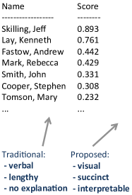
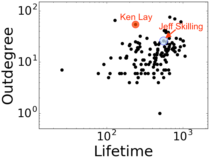
Figure 1: LookOut explains Enron founder/CEO “Ken Lay” and COO “Jeff Skilling” by two “pair plots” in which they are most salient. Compared to traditional ranked list output (left), LookOut produces simpler, more interpretable explanations (right).

Anomaly detection is a widely studied problem. Numerous detectors exist for point data [2, 6, 19], time series [13], as well as graphs [3, 4]. However, the literature on anomaly explanation or description is perhaps surprisingly sparse. Given that the outcomes (i.e. alerts) of a detector often go through a “vetting” procedure by human analysts, it is extremely beneficial to provide explanations for such alerts which can empower analysts in sensemaking and reduce their efforts in troubleshooting and recovery. Moreover, such explanations should justify the anomalies as succinctly as possible in order to save analyst time.

Our work sets out to address the anomaly explanation problem, with a focus on time-evolving graphs. Consider the following example situation: Given the IP-IP communications over time from an institution, a network analyst could face two relevant scenarios.

• Detected anomalies: For monitoring, s/he could use any “black-box” anomaly detector to spot suspicious IPs. Here, we are oblivious to the specific detector, knowing only that it flags anomalies, but does not produce any interpretable explanation.

• Dictated anomalies: Alternatively, anomalous IPs may get reported to the analyst externally (e.g., they crash or get compromised).

In both scenarios, the analyst would be interested in understanding in what ways the pre-identified anomalous IPs (detected or dictated) differ from the rest.

In this work, we propose a new approach called LookOut, for explaining a given set of anomalies, and apply it to the scope of $t$-graphs. At its heart, LookOut provides interpretable visual explanations through simple, easy-to-grasp plots, which “incriminate” the given anomalies the most. We summarize our contributions as follows.

• Anomaly Explanation Problem Formulation: We introduce a new formulation that explains anomalies through “pair plots”. In a nutshell, given the list of anomalies from a $t$-graph, we aim to find a few pair plots on which the total “blame” that the anomalies receive is maximized. Our emphasis is on two key aspects: (a) interpretability: our plots visually incriminate the anomalies, and (b) succinctness: we show only a few plots to respect the analyst’s attention; the analysts can then quickly interpret the plots, spot the outliers, and verify their abnormality given the discovered feature pairs.

• Succinct Explanation Algorithm LookOut: We propose the LookOut algorithm to solve our explanation problem. Specifically, we develop a plot selection objective that lends itself to monotone submodular function optimization, which we solve efficiently with optimality guarantees. Figure 1 illustrates LookOut’s performance on the Enron communications network, where it discovers two pair plots which maximally incriminate the given anomalous nodes: Enron founder “Ken Lay” and CEO “Jeff Skilling.” Note that the anomalies stand out visually from the normal nodes.

• Generality: LookOut is general in two respects: it is (a) domain-agnostic, meaning it is suitable for real-world $t$-graphs from various domains that involve human actors, and (2) detector-agnostic, meaning it can be employed to explain anomalies produced by any detector or identified through any other mechanism (e.g., crash reports, customer complaints, etc.)

• Scalability: We show that LookOut requires time linear on the number of edges in the input $t$-graph, which is simply the cost incurred to compute feature values. In fact, the pair plot scoring and selection steps are carefully designed to add only a constant cost, which is independent of graph size (see Lemma 3.1 and Fig. 4).

We experiment with real $t$-graph datasets from diverse domains including e-mail and IP-IP communications, as well as co-authorships over time, which demonstrate the effectiveness, interpretability, succinctness and generality of our approach.

Reproducibility: LookOut is open-sourced at https://github.com/NikhilGupta1997/Lookout, and our datasets are publicly available (See Section 4.1).

2 Preliminaries and Problem Statement

Table 1: Symbols and Definitions

Symbol	Definition
$\mathcal{G}$	Input graph, $\mathcal{G}=(\mathcal{V},\mathcal{E})$, $|\mathcal{V}|=n,|\mathcal{E}|=m$
$\mathcal{A}$	Input anomalies, $|{\mathcal{A}}|=k$
$\mathcal{F}$	Set of node features, $|{\mathcal{F}}|=d$
$\mathcal{P}$	Set of pair plots, $|{\mathcal{P}}|=d(d-1)/2=l$
${s}_{i,j}$	Anomaly score of $a_{i}\in{\mathcal{A}}$ in plot $p_{j}\in{\mathcal{P}}$
$\mathcal{S}$	Subset of selected plots
$f(\mathcal{S})$	Explanation objective function
$\Delta_{f}(p\ |\ \mathcal{S})$	Marginal gain of plot $p$ w.r.t $\mathcal{S}$
$b$	Budget, i.e., maximum cardinality of $\mathcal{S}$

2.1 Notation

Formally, a $t$-graph is a collection of time-ordered edges $\mathcal{G}({\mathcal{V}_{s}}\cup{\mathcal{V}_{d}},{\mathcal{E}})=\{e_{1},e_{2},\ldots\}$ where each edge $e\in{\mathcal{E}}$ is a tuple $\langle v_{s},v_{d},ts,val\rangle$. Here, $v_{s}\in{\mathcal{V}_{s}}$ and $v_{d}\in{\mathcal{V}_{d}}$ are the source and destination nodes of $e$, $ts$ is the time stamp associated with $e$, and $val$ is a value on $e$. For unipartite graphs (like IP-IP) ${\mathcal{V}_{s}}={\mathcal{V}_{d}}$, and for bipartite graphs (like user-ATM) ${\mathcal{V}_{s}}\cap{\mathcal{V}_{d}}=\emptyset$. Edge value could be categorical (edge type, e.g., withdrawal vs. deposit) or numerical (edge weight, e.g., dollar amount). We denote the number of nodes by $|{\mathcal{V}_{s}}\cup{\mathcal{V}_{d}}|=|{\mathcal{V}}|=n$. We refer to the number of edges $|{\mathcal{E}}|=m$ as the size of $\mathcal{G}$. Note that such graphs can be considered multigraphs, as multiple edges between $v_{s}$ and $v_{d}$ are permitted.

The set of anomalous nodes given as input is denoted by ${\mathcal{A}}\subset{\mathcal{V}}$, $|{\mathcal{A}}|=k$. For bipartite graphs, anomalies could be suspicious sources (e.g., users) ${\mathcal{A}}\subset{\mathcal{V}_{s}}$ or destinations (e.g., ATMs) ${\mathcal{A}}\subset{\mathcal{V}_{d}}$.

To characterize the anomalies in $t$-graphs, we use a list of features for each node, denoted by ${\mathcal{F}}=\{f_{1},f_{2},\ldots,f_{d}\}$. We describe our node features next.

2.2 Features for $t$-graphs

We characterize the nodes in a time-evolving graph with numerical properties they exhibit, and explain node anomalies using these derived features. The literature is rich on feature extraction from graphs [3, 14, 11, 25, 24, 12].

Oddball [3] introduced and successfully used various relational features for anomaly detection in static weighted graphs. We leverage several of these features including (1) indegree, (2) outdegree, (3) inweight-v, and (4) outweight-v, where weight of an edge $\langle v_{s},v_{d},ts,val\rangle$ is the value $val$. Since we work with temporal graphs, we also use (5) inweight-r and (6) outweight-r, where edge weight depicts the number of repetitions of the edge (multi-edge).

In addition to structure, we have the time information. To this end, we leverage the inter-arrival times (IAT) between the edges. IAT distributions have been successfully used in a number of prior works on fraud detection [11, 25]. We specifically use: IAT (7) average, (8) variance, (9-11) minimum, median, and maximum. We also define (12) lifetime, the gap between the first and the last edge.

Admittedly, there are numerous other features one could extract from graphs. In this work, our focus is on the explanation problem, and thus we mainly build on existing features that were shown to be useful in prior anomaly and fraud detection tasks. One could easily extend our list with others, such as recursive structural features [14] or node embeddings [24, 12], but we recommend using interpretable features that have direct meanings for analyst benefit, as well as scalable to compute for large graphs.

2.3 Intuition & Proposed Problem

The explanations we seek to generate should be simple and interpretable. Moreover, they should be easy to illustrate to humans who will ultimately leverage the explanations. To this end, we decide to use “pair plots” (=scatter plots) for anomaly justification, due to their visual appeal and interpretability. That is, we consider ${d\choose 2}=\frac{d(d-1)}{2}$ 2-d spaces by generating all pairwise feature combinations. Within each 2-d space, we then score the nodes in ${\mathcal{A}}$ by their anomalousness (Section 3.1).

Let us denote the set of all $d\choose 2$ pair plots by ${\mathcal{P}}$. Even for small values of $d$, showing all the pair plots would be too overwhelming for the analyst. Moreover, some anomalies could redundantly show up in multiple plots. Ideally, we would identify only a few pair plots, which could “blame” or “explain away” the anomalies to the largest possible extent. In other words, our goal would be to output a small subset ${\mathcal{S}}$ of ${\mathcal{P}}$, on which nodes in ${\mathcal{A}}$ receive high anomaly scores (Section 3.2).

Given this intuition, we formulate our problem:

Problem 1 (Anomaly Explanation)

• Given

  • a list of anomalous nodes ${\mathcal{A}}\subset{\mathcal{V}}$ from a $t$-graph, either (1) detected by an off-the-shelf detector or (2) dictated by external information, and

  • a fixed budget of $b$ pair plots;

• find the best such pair plots ${\mathcal{S}}\subset{\mathcal{P}}$, $|{\mathcal{S}}|=b$

• to maximize the total maximum anomaly score of anomalies that we can “blame” through the $b$ plots.

3 Proposed Algorithm LookOut

In this section, we detail our approach for scoring the input anomalies by pair plots, our selection criterion and algorithm for choosing pair plots, the overall complexity analysis of LookOut, and conclude with discussion.

3.1 Scoring by Feature Pairs

Given all the nodes ${\mathcal{V}}$, with marked anomalies ${\mathcal{A}}\subset{\mathcal{V}}$, and their extracted features ${\mathcal{F}}\in\mathbb{R}^{d}$, our first step is to quantify how much “blame” we can attribute to each input anomaly in $\mathbb{R}^{2}$. As previously mentioned, 2-d spaces are easy to illustrate visually with pair plots. Moreover, anomalies in 2-d are easy to interpret: e.g., “point $a$ has too many/too little $y$=dollars for its $x$=number of accounts”. Given a pair plot, an analyst can easily discern the anomalies visually, and come up with such explanations without any further supervision.

We construct 2-d spaces $(f_{x},f_{y})$ by pairing the features $\forall x,y=\{1,\ldots,d\},x\neq y$. Each pair plot $p_{j}\in{\mathcal{P}}$ corresponds to such a pair of features, $j=\{1,\ldots,{d\choose{2}}\}$. For scoring, we consider two different scenarios, depending on how the input anomalies were obtained.

If the anomalies are detected by some “black-box” detector available to the analyst, we can employ the same detector on all the nodes (this time in 2-d) and thus obtain the scores for the nodes in ${\mathcal{A}}$.

If the anomalies are dictated, i.e. reported externally, then the analyst could use any off-the-shelf detector, such as LOF [6], DB-outlier [16], etc. In this work, we use the Isolation Forest (iForest) detector [19] for two main reasons: (a) it boasts constant training time and space complexity due to its sampling strategy, and (b) it has been shown empirically to outperform alternatives [10] and is thus state-of-the-art. However, note that none of these existing detectors has the ability to explain the outliers, especially iForest, as it is an ensemble approach.

By the end of the scoring process, each anomaly receives a total of $|{\mathcal{P}}|=l$ scores.

3.2 Explaining by Pair Plots

While scoring in small, 2-d spaces is easy and can be trivially parallelized, presenting all such pair plots to the analyst would not be productive given their limited attention budget. As such, our next step is to carefully select a short list of plots that best blame all the anomalies collectively, where the plot budget can be specified by the user.

While selecting plots for justification, we aim to incorporate the following criteria:

• incrimination power; such that the anomalies are scored as highly as possible,

• high expressiveness; where each plot incriminates multiple anomalies, so that the explanation is sublinear in the number of anomalies, and

• low redundancy; such that the plots do not repeatedly explain similar sets of anomalies.

We next introduce our objective criterion which satisfies the above requirements.

3.2.1 Objective function

At this step of the process, we can conceptually think of a complete, weighted bipartite graph between the $k$ input anomalies $\mathcal{A}=\{{a_{1},\dotsc,a_{k}}\}$ and $l$ pair plots $\mathcal{P}=\{{p_{1},\dotsc,p_{l}}\}$, in which edge weight $s_{i,j}$ depicts the anomaly score that $a_{i}$ received from $p_{j}$, as illustrated in Fig. 2.

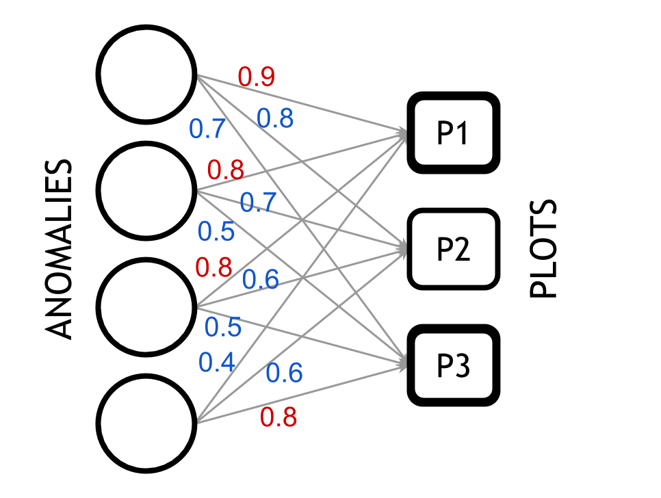
Figure 2: LookOut selection with $k=4$ anomalies, $l=3$ plots, and budget $b=2$. P1 is picked first due to maximum total incrimination (2.9) (sum of incoming edge weights). Next P3 is chosen over P2, due to higher marginal gain (0.4 vs 0.2).

We formulate our objective to maximize the total maximum score of each anomaly amongst the selected plots, as given in Eq. (3.1):

(3.1) $${\max_{{{\mathcal{S}}\subset{\mathcal{P}},|{\mathcal{S}}|=b}}}\;\;\;f(\mathcal{S})=\sideset{}{\limits{}_{a_{i}\in\mathcal{A}}}{\sum}\;\;\max_{p_{j}\in\mathcal{S}}\;s_{i,j}$$

Here, $f({\mathcal{S}})$ can be considered the total incrimination score given by subset ${\mathcal{S}}$. Since we are limited with a budget of plots, we aim to select those which explain multiple anomalies to the best extent. Note that each anomaly receives their maximum score from exactly one of the plots among the selected set, which effectively partitions the explanations and avoids redundancy. In the example Fig. 2, P1 and P3 “explain away” anomalies $\{1,2,3\}$ and $\{4\}$ respectively, where the maximum score that each anomaly receives is highlighted in red font.

Concretely, we denote by ${\mathcal{A}}_{p}$ the set of anomalies that receive their highest score from $p$, i.e. ${\mathcal{A}}_{p}=\{a_{i}|p=\max_{p_{j}\in\mathcal{S}}\;s_{i,j}\}$, where we break ties at random. Note that ${\mathcal{A}}_{p}\cap{\mathcal{A}}_{p^{\prime}}=\emptyset,\;\forall p,p^{\prime}\in{\mathcal{P}}$. In depicting a plot $p$ to the analyst, we mark all anomalies in ${\mathcal{A}}_{p}$ in red and the rest in ${\mathcal{A}}\backslash{\mathcal{A}}_{p}$ in blue – c.f. Fig. 1.

3.2.2 Subset selection

Algorithm 1 LookOut

0:  anomalies $\mathcal{A}$, plots ${\mathcal{P}}$, budget $b$

0:  set of selected plots $\mathcal{S}$

1:  initialize $\mathcal{S}\to\emptyset$

2:  calculate $\Delta_{f}(p\ |\ \mathcal{S})\ \forall\ p\in\mathcal{P}$

3:  generate sorted queue $Q$ on marginal gains

4:  while $|\mathcal{S}|<b$ do

5:     $p_{top}:=$ pop from $Q$

6:     update $\Delta_{f}(p_{top}\ |\ \mathcal{S})$

7:     if $\Delta_{f}(p_{top}\ |\ \mathcal{S})\geq$ top of $Q$ {ranks top} then

8:        $\mathcal{S}:=\mathcal{S}\cup\{p_{top}\}$

9:     else

10:        insert $p_{top}$ in $Q$ with updated $\Delta_{f}(p_{top}\ |\ \mathcal{S})$

11:     end if

12:  end while

13:  return  $\mathcal{S}$

Having defined our explanation objective, we need to devise a subset selection algorithm to optimize Eq. (3.1), for a budget $b$. Note that optimal subset selection is a combinatorial task.

Fortunately, our objective $f(\cdot)$ exhibits three key properties that enable us to use a greedy algorithm with an approximation guarantee. Specifically, we can show that our set function $f:2^{\mathcal{P}}\rightarrow\mathbb{R}_{+}$ is

1. non-negative; since the anomaly scores take non-negative values, often in $[0,1]$;

2. monotonic; as for every $\mathcal{S}\subseteq\mathcal{T}\subseteq\mathcal{P}$, $f(\mathcal{S})\leq f(\mathcal{T})$. That is, adding more plots to a set cannot decrease the maximum score attributed to any anomaly;

3. and submodular; since for every $\mathcal{S}\subseteq\mathcal{T}\subseteq\mathcal{P}$ and for all $p\in\mathcal{P}\backslash\mathcal{T}$, $f(\mathcal{S}\cup\{p\})-f(\mathcal{S})\geq f(\mathcal{T}\cup\{p\})-f(\mathcal{T})\;.$ That is, adding any plot $p$ to a smaller set can increase the function value at least as much as adding it to its superset.

We give the submodularity proof in Appendix A, as non-negativity and monotonicity are trivial to show.

Submodular functions with non-negativity and monotonicity properties admit approximation guarantees under a greedy approach identified by Nemhauser et al. [22]. The greedy algorithm starts with the empty set ${\mathcal{S}}_{0}$. In iteration $t$, it adds the element (in our case, pair plot) that maximizes the marginal gain $\Delta_{f}$ in function value, defined as

$$\Delta_{f}(p|{\mathcal{S}}_{t-1})=f({\mathcal{S}}_{t-1}\cup\{p\})-f({\mathcal{S}}_{t-1})\;.$$

That is,

$${\mathcal{S}}_{t}:={\mathcal{S}}_{t-1}\cup\{\arg\max_{p\in\mathcal{P}\backslash{\mathcal{S}}_{t-1}}\Delta_{f}(p|{\mathcal{S}}_{t-1})\}\;.$$

Based on their proof, one can show that when $t=b$,

$$f({\mathcal{S}}_{b})\geq\big{(}1-\frac{1}{e}\big{)}\max_{|{\mathcal{S}}|\leq b}f({\mathcal{S}})\;.$$

In other words, the simple greedy search heuristic achieves at least $63$% of the objective value of the optimum set.

Algorithm 1 shows the psuedocode of our LookOut pair plot selection process.

3.3 Complexity Analysis

Lemma 3.1

LookOut scales linearly in terms of the input size, i.e. number of edges in the input $t$-graph.

• The complexity of feature extraction (Section 2.2) is the most computationally demanding part of LookOut, and requires time linear on the number of edges in the graph—since all features are defined on the incident edges per node.

  We show that the other two parts—scoring the given anomalies (Section 3.1) and selecting pair plots to present (Section 3.2)—add only a constant time, and are independent of the graph size.

  Let us denote by $d$ the number of features we extract. For scoring, we generate 2-d representations by pairing the features. For each pair, we train an iForest model in 2-d. Following their recommended setup, we typically sample $256$ points (i.e., nodes) from the data and train around $t=100$ extremely randomized trees, called isolation trees. The complexity of training an iForest is $O(t\psi\log\psi)$, and scoring a set of $|{\mathcal{A}}|=k$ anomalous points takes $O(tk\log\psi)$. The total scoring complexity is thus $O(d^{2}t(k+\psi)\log\psi)$, and is independent of the total number of nodes or edges in the input graph.

  At last, we employ the greedy selection algorithm, where we compute the marginal gain of adding each plot to our select-set, which takes $O(d^{2}k)$ and pick the plot with the largest gain through a linear scan in $O(d^{2})$. We repeat this process $b$ times until the budget is exhausted. The total selection complexity is thus $O(d^{2}kb)$, which is also independent of graph size.

  Thus, having extracted the features in $O(m)$, LookOut takes constant additional time to produce its output, where all of $\{d,\psi,t,k,b\}$ are (small) constants in practice. $\blacksquare$

3.4 Discussion

Here we answer some questions that may be in the reader’s mind.

1. How do we define “anomaly?” We defer this question to the off-the-shelf anomaly detection algorithm (iForest [19], LOF [6], DB-outlier [16], etc.) Our focus here is to succinctly and interpretably show what makes the pre-selected items stand out from the rest.

2. Why pair plots? Using pair plots for justification is an essential, concious choice we make for several reasons: (a) scatterplots are easy to look at and quickly interpret (b) they are universal and non-verbal, in that we need not use language to convey the anomalousness of points – even people unfamiliar with the context of Enron will agree that the point “Jeff Skilling” in Fig. 1 is far away from the rest, and (c) they show where the anomalies lie relative to the normal points – the contrastive visualization of points is more convincing than stand-alone rules.

3. How do we choose the budget? We designed our explanation objective to be budget-conscious, and let the budget be specified by the analyst. In general, humans have a working memory of size “seven, plus or minus two” [21].

4 Experiments

In this section, we empirically evaluate LookOut on three, diverse datasets. Our experiments were designed to answer the following questions:

1. Quality of Explanation: How well can LookOut “explain” or “blame” the given anomalies?

2. Scalability: How does LookOut scale with the input graph size and the number of anomalies?

3. Discoveries: Does LookOut lead to interesting and intuitive explanations on real world data?

These are addressed in Sec. 4.3, 4.4 and 4.5 respectively. Before detailing our empirical findings, we describe the datasets used and our experimental setup.

4.1 Dataset Description

To illustrate the generality of our proposed domain-agnostic $t$-graph features and LookOut itself, we select our datasets from diverse domains: e-mail communication (Enron), co-authorship (DBLP) and computer (LBNL) networks. These datsets are publicly available, unipartite directed graphs. We describe them below and provide a summary in Table 2.

Table 2: Datasets studied.

Dataset	Nodes	Edges	Time	Descrip.
Enron [26]	151	20K	3 yrs	email comm.
DBLP [1]	1.3M	19M	25 yrs	coathorship
LBNL [23]	2.5K	0.2M	1 hr	IP-IP comm.

Enron: This dataset consists of 19K emails exchanged between 151 Enron employees during the period surrounding the scandal (May 1999-June 2002). The communications are on daily granularity.

LBNL: This dataset details network traffic between 2.5K computers during a one hour interval known to contain network attacks (e.g., port scans). Traffic is recorded at second granularity.

DBLP: This dataset contains the co-authorship network of 1.3M authors over 25 years from 1990 to 2014. The networks are collected at yearly granularity.

4.2 Experimental Setup

To obtain “ground-truth” anomalies for LookOut input, we use the iForest [19] algorithm on features described in Sec. 2.2 for each $t$-graph. This yields a ranked list of points with scores in $[0,1]$ (higher value suggests higher abnormality), from which we pick the desired top $k$. Analogously, we use iForest for computing the anomaly score in each pair plot. We note that the analyst is free to choose any anomaly detector(s) for both/either of the above stages, making LookOut detector-agnostic. However, it is recommended that the same methods be used for both stages to ensure ranking similarities.

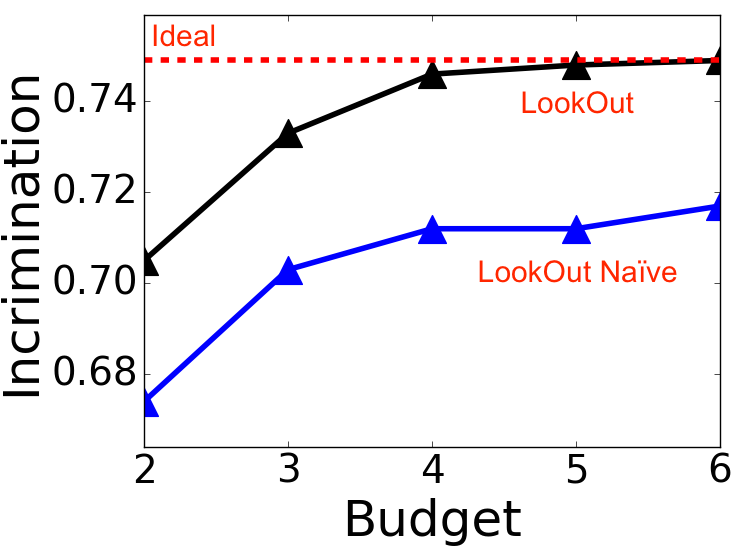
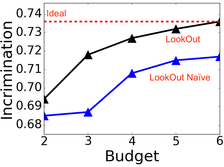
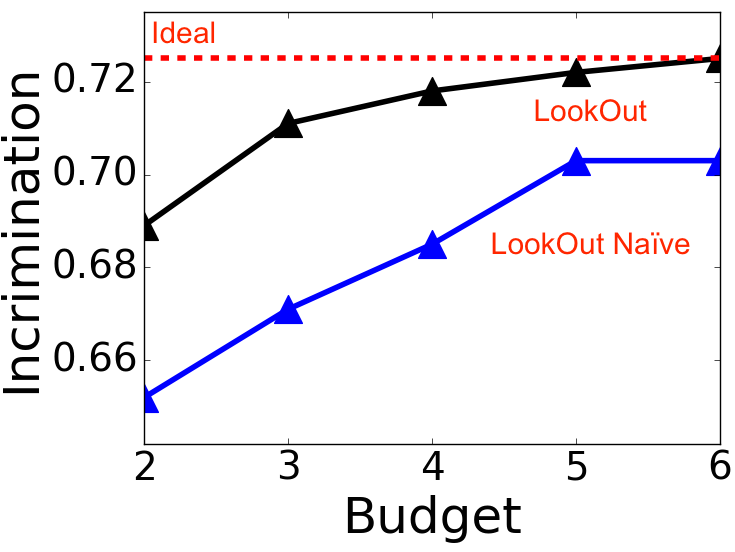
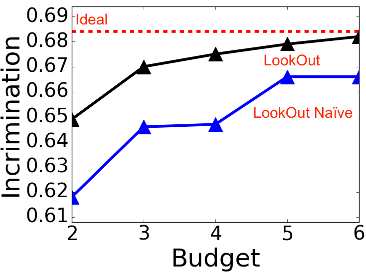
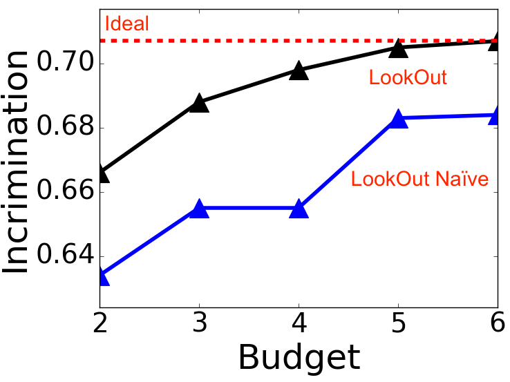
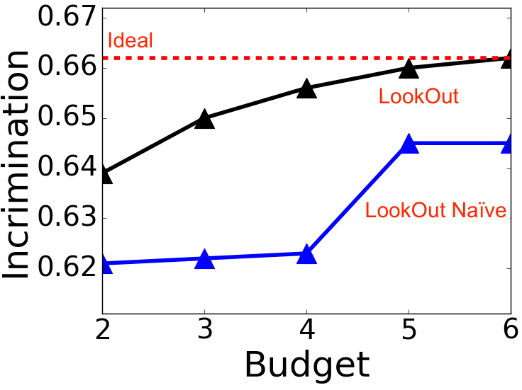
Figure 3: LookOut explains away top 10-30 anomalies with 4-5 plots. Results shown on LBNL (left) and Enron (right) with $k=\{10,20,30\}$ anomalies (top to bottom).

4.3 Quality of Explanation

We quantify the quality of explanation provided by a set of plots ${\mathcal{S}}$ through their incrimination score:

(4.2) $$\textit{incrimination}({\mathcal{S}})=\frac{f(\mathcal{S})}{\left|{\mathcal{A}}\right|}$$

where ${\mathcal{A}}$ is the set of input anomalies and $f(\cdot)$ is the objective funtion defined in Eq. 3.1. Intuitively, incrimination is the average maximum blame that an input anomaly receives from any of the selected plots.

Due to the lack of comparable prior works, we use a naïve version of our approach, called LookOut-Naïve which ignores the submodularity of our objective. Instead, LookOut-Naïve assigns a score to each plot by summing up scores for all given anomalies and chooses the top $b$ plots for a given budget $b$.

Fig. 3 compares the incrimination scores of both LookOut-Naïve and LookOut on the Enron and LBNL datasets for several choices of $k$ and $b$. The red dotted line indicates the ideal value, $f({\mathcal{P}})$, i.e., the highest achievable incrimination (by selecting all plots). Fig. 3 shows that LookOut consistently outperforms LookOut-Naïve and rapidly converges to the ideal incrimination with increasing budget. Results on DBLP were similar, but excluded for space constraints.

4.4 Scalability

We empirically studied how LookOut runtime varies with (i) the graph size $m$ and (ii) the number of anomalies $k$. All experiments were performed on an OSX personal computer with 16GB memory. Runtimes were averaged over 10 trials.

To measure scalability with respect to graph size, we sampled edges from $[100K,10M]$ in logarithmic intervals from DBLP while fixing budget to $b=5$ and $k=50$ anomalies. Fig. 4 (left) plots runtime vs. number of edges, demonstrating a linear fit with slope $\approx$ 1. This empirically confirms Lem. 3.1.

We also study the variation of runtime with the number of anomalies, as feature extraction incurs a constant overhead on each dataset. Fig. 4 (right) illustrates linear scaling with respect to number of anomalies for a DBLP subgraph with 10K edges.

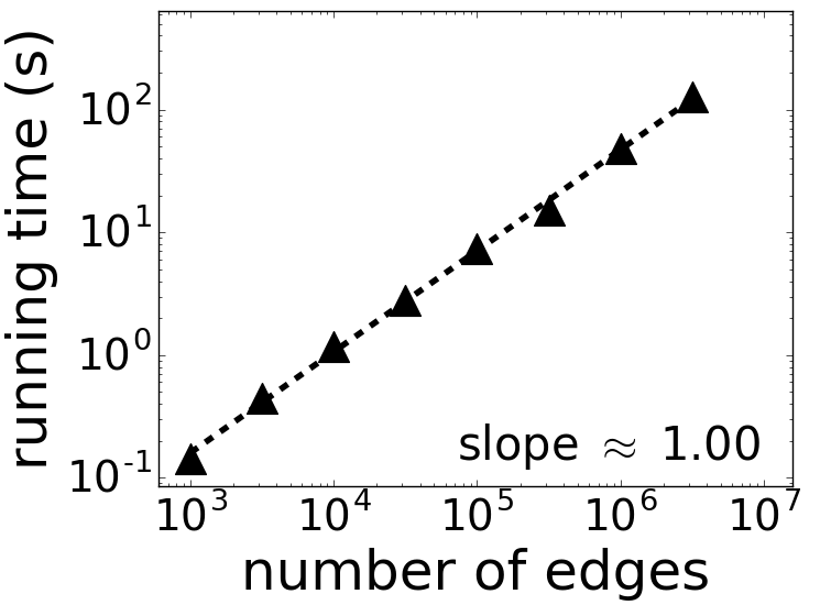
Figure 4: LookOut scales linearly with number of edges (left) and number of anomalies (right).

4.5 Discoveries

(a)	(b)
(c)	(d)
(e)	(f)

Figure 5: Discoveries using LookOut on detected anomalies: LookOut partitions and explains anomaly detection results from iForest on DBLP (a-b) and LBNL (c-f) datasets.

In this section, we present our discoveries using LookOut on all three real world datasets. Scoring in 2-d was performed using iForest with $t=100$ trees and sample size $\psi=64$ (Enron) and $\psi=256$ (LBNL and DBLP). We use dictated anomalies for Enron, and detected anomalies for LBNL and DBLP datasets to demonstrate performance in both settings.

Enron: We used two top actors in the Enron scandal, Kenneth Lay (CEO) and Jeff Skilling (CFO) as dictated anomalies for LookOut and sought explanations for their abnormality based on internal e-mail communications. With $b$=2, LookOut produced the plots shown in Fig. 1 (right). Explanations indicate that Jeff Skilling had an unsually large IAT-max for the number of employees he communicated with (outdegree). On the other hand, Kenneth Lay sent emails to an abnormally large number of employees (outdegree) given the time range during which he emailed anyone (lifetime).

DBLP: We obtained ground truth anomalies by running iForest on the high-dimensional space spanned by a subset of features from Sec. 2.2. With $k=5$, the detected anomalous authors were Alberto L. Sangiovanni-Vincentelli, H. Vincent Poor, Hao Wang, Jack Dongarra and Thomas S. Huang. The explanations provided by LookOut with $b=2$ are shown in Fig. 5a-b. Thus, the anomalous authors users are partitioned into two groups. The members of the first group, Alberto L. Sangiovanni-Vincentelli, H. Vincent Poor, Jack Dongarra, and Thomas S. Huang are anomalous because they had usually high duration during which they published papers (lifetime) and total number of co-authorships (inweight-r). This is consistent with their high h-indices obtained from their respective google scholar pages (see brackets in Fig. 5a). The second group consists of only Hao Wang, who was also anomalous in this plot, but is best explained by very high IAT-variance for his inweight-r value, shown in Fig. 5b.

LBNL: We ran LookOut with $k$=10 and $b$=4 and obtained the output pair plots as shown in Fig. 5c-f. We observe the different anomalous nodes that have been incriminated differently depending on the pair plot. Port 524 is highlighted in Fig. 5c due to its very low IAT-avg and IAT-variance hinting at it being hotspot port with a large number of transmissions at a quick continuous rate.

Fig. 5d shows 4 anomalies including Port 515 and Port 4201. In fact, Port 515 handles requests based on the Line Printer Daemon Protocol which establishes network printing services. Our observations of a high IAT-min over a long lifetime are in tandem with print requests being polled over the network at fixed time intervals.

Fig. 5e incriminates Port 80, Port 443 and Port 5730. Port 80 is the designated port for the internet hypertext transfer protocol (HTTP) and helps retrieve HTML data from web servers. As such, we observe that Port 80 has an extremely high indegree and outdegree, indicating that this port is used for a large number of diverse connections between several web servers. Its contemporary counterpart Port 443 is assigned for secure communications (HTTPS) and is thus incriminated for the same identifying reasons as the former.

Port 2888 in Fig. 5f is used by ZooKeeper, a centralized coordination service for distributed applications like Hadoop . It appears with an abnormally low lifetime and IAT-variance probably indicating a small active transmission time which involved a quick configuration broadcast between devices.

Note that on all datasets, anomalous points are clearly visually distinguishable, and often complementary between pair plots. This is in line with our desired explanation task, and achieved as a result of our LookOut subset selection objective and approach.

5 Related Work

While there is considerable prior work on anomaly detection [7, 4, 13], literature on anomaly description is comparably sparse. Several works aim to find an optimal feature subspace which distinguishes anomalies from normal points. [15] aims to find a subspace which maximizes differences in anomaly score distributions of all points across subspaces. [18] instead takes a constraint programming approach which aims to maximize differences between neighborhood densities of known anomalies and normal points. An associated problem focuses on finding minimal, or optimal feature subspaces for each anomaly. [16] aims to give “intensional knowledge” for each anomaly by finding minimal subspaces in which the anomalies deviate sufficiently from normal points using pruning rules. [8, 9] use spectral embeddings to discover subspaces which promote high anomaly scores, while aiming to preserve distances of normal points. [20] instead employs sparse classification of an inlier class against a synthetically-created anomaly class for each anomaly in order to discover small feature spaces which discern it. [17] proposes combining decision rules produced by an ensemble of short decision trees to explain anomalies. [5] augments the per-outlier problem to include outlier groups by searching for single features which differentiate many outliers.

All in all, none of these works meet several key desiderata for anomaly description: (a) quantifiable explanation quality, (b) budget-consciousness towards analysts (returning explanations which do not grow with size of the anomalous set), (c) visual interpretability, and (d) a scalable descriptor, which is sub-quadratic on the number of nodes and at worst polynomial on (low) dimensionality. Table 3 shows that unlike existing approaches, our LookOut approach is designed to give quantifiable explanations which aim to maximize incrimination, respect human attention-budget and visual interpretability constraints, and scale linearly on the number of graph edges.

Table 3: Comparison with other anomaly description approaches, in terms of four desirable properties.

Properties vs. Methods	Knorr et al. [16]	Dang et al.[8]	Angiulli et al. [5]	Micenkova et al. [20]	Kopp et al. [17]	Keller et al. [15]	LookOut
Quantifiable Explanations		✔	✔	✔		✔	✔
Budget-conscious						✔	✔
Visually Interpretable							✔
Scalable		✔			✔	✔	✔

6 Conclusions

In this work, we formulated and tackled the problem of succinctly and interpretably explaining anomalies in $t$-graphs to human analysts. We identified a number of domain-agnostic features of $t$-graphs, and subsequently made the following contributions: (a) problem formulation: we formulate our goal for explaining anomalies using a budget of visually interpretable pair plots, (b) explanation algorithm: we propose a submodular objective to quantify explanation quality and propose the LookOut method for solving it approximately with guarantees, (c) generality: we show that LookOut can work with diverse domains and any detection algorithm, and (d) scalability: we show theoretically and empirically that LookOut scales linearly in the size of the input graph. We conduct experiments on real e-mail communication, co-authorship and IP-IP interaction $t$-graphs and demonstrate that LookOut produces qualitatively interpretable explanations for “ground-truth” anomalies and achieves strong quantitative performance in maximizing our proposed objective.

A Proof of Submodularity

Our explanation objective is defined as:

$${\max_{{{\mathcal{S}}\subset{\mathcal{P}},|{\mathcal{S}}|=b}}}\;\;\;f(\mathcal{S})=\sideset{}{\limits{}_{a_{i}\in\mathcal{A}}}{\sum}\;\;\max_{p_{j}\in\mathcal{S}}\;s_{i,j}$$

Next we show that the set function $f$ is submodular.

• Consider two sets $\mathcal{S}$ and $\mathcal{T}$, $\mathcal{S}\subseteq\mathcal{T}\subseteq\mathcal{P}$, and the function,

  $$\mathcal{F}(p_{k},\mathcal{S},\mathcal{T})=\Delta_{f}(p_{k}\ |\ \mathcal{S})-\Delta_{f}(p_{k}\ |\ \mathcal{T})\;.$$

  By definition of submodularity, function $f$ is submodular if and only if,

  $$\mathcal{F}(p_{k},\mathcal{S},\mathcal{T})\geq 0\;\;\forall\ p_{k}\in\mathcal{P}\setminus\mathcal{T}\;.$$

For simplicity lets write $\mathcal{F}$ as,

$$\mathcal{F}(p_{k},\mathcal{S},\mathcal{T})=\sideset{}{{}_{a_{i}\in\mathcal{A}}}{\sum}t_{i}$$

where each term $t_{i}$ is given as

$$$$t_{i}=[\max(s_{i,k},\max\limits_{p_{j}\in\mathcal{S}}s_{i,j})\ -\max(s_{i,k},\max\limits_{p_{j}\in\mathcal{T}}s_{i,j}\\ +\max\limits_{p_{j}\in\mathcal{T}}\;s_{i,j}-\max\limits_{p_{j}\in\mathcal{S}}\;s_{i,j}]\;.$$$$

Now we consider the following three cases:

Case 1

For some $a_{i}\in\mathcal{A}\ \exists\ p_{j^{\prime}}\in\mathcal{S}$ s.t. $s_{i,j}\geq s_{i,k}$, then,

$$\max(s_{i,k},\max\limits_{p_{j}\in\mathcal{S}}s_{i,j})=\max\limits_{p_{j}\in\mathcal{S}}s_{i,j}\;,$$

and similarly since $\mathcal{S}\subseteq\mathcal{T},\ p_{j^{\prime}}\in\mathcal{T}$

$$\max(s_{i,k},\max\limits_{p_{j}\in\mathcal{T}}s_{i,j})=\max\limits_{p_{j}\in\mathcal{T}}s_{i,j}\;.$$

$\therefore$  for all such $a_{i}\in\mathcal{A},\ t_{i}=0\;.$

Case 2

For some $a_{i}\in\mathcal{A}\ \nexists\ p_{j^{\prime}}\in\mathcal{S}$ s.t. $s_{i,j^{\prime}}\geq s_{i,k}$ and $\exists\ p_{j^{\prime}}\in\mathcal{T}$ s.t. $s_{i,j^{\prime}}\geq s_{i,k}$ , then,

$$\max(s_{i,k},\max\limits_{p_{j}\in\mathcal{S}}s_{i,j})=s_{i,k}$$

and conversely,

$$\max(s_{i,k},\max\limits_{p_{j}\in\mathcal{T}}s_{i,j})=\max\limits_{p_{j}\in\mathcal{T}}s_{i,j}$$

$\therefore$  for all such $a_{i}\in\mathcal{A},$ $t_{i}=s_{i,k}-\max\limits_{p_{j}\in\mathcal{S}}s_{i,j}\geq 0\;.$

Case 3

For some $a_{i}\in\mathcal{A}\ \nexists\ p_{j^{\prime}}\in\mathcal{T}$ s.t. $s_{i,j^{\prime}}>s_{i,k}$, then,

$$\max(s_{i,k},\max\limits_{p_{j}\in\mathcal{T}}s_{i,j})=s_{i,k}$$

and similarly since $\mathcal{S}\subseteq\mathcal{T}$,

$$\max(s_{i,k},\max\limits_{p_{j}\in\mathcal{S}}s_{i,j})=s_{i,k}\;.$$

$\therefore$  for all such $a_{i}\in\mathcal{A}$,

$$$$t_{i}=\max\limits_{p_{j}\in\mathcal{T}}s_{i,j}-\max\limits_{p_{j}\in\mathcal{S}}s_{i,j}\geq 0\ \ (\because\mathcal{A}\subseteq\mathcal{B})$$$$

As a result of all three possible cases we see that $t_{i}\geq 0\ \forall\ a_{i}\in\mathcal{A}$. Hence,

$$\mathcal{F}(p_{k},\mathcal{S},\mathcal{T})=\sideset{}{{}_{a_{i}\in\mathcal{A}}}{\sum}t_{i}\geq 0$$

$$\therefore\ \ \mathcal{F}(p_{k},\mathcal{S},\mathcal{T})\geq 0\ \forall\ p_{k}\in\mathcal{P}\setminus\mathcal{T}$$

We conclude that the set function $f$ is submodular. $\blacksquare$

References

- [1] Dblp network dataset. 2014.
- [2] C. C. Aggarwal. Outlier Analysis. Springer, 2013.
- [3] L. Akoglu, M. McGlohon, and C. Faloutsos. Oddball: Spotting anomalies in weighted graphs. PAKDD, pages 410–421, 2010.
- [4] L. Akoglu, H. Tong, and D. Koutra. Graph based anomaly detection and description: a survey. Data Min. Knowl. Discov., 29(3):626–688, 2015.
- [5] F. Angiulli, F. Fassetti, and L. Palopoli. Discovering characterizations of the behavior of anomalous subpopulations. IEEE TKDE, 25(6):1280–1292, 2013.
- [6] M. M. Breunig, H.-P. Kriegel, R. T. Ng, and J. Sander. LOF: Identifying density-based local outliers. SIGMOD Rec., 29(2):93–104, 2000.
- [7] V. Chandola, A. Banerjee, and V. Kumar. Anomaly detection: A survey. ACM Computing Surveys (CSUR), 41(3):15, 2009.
- [8] X. H. Dang, I. Assent, R. T. Ng, A. Zimek, and E. Schubert. Discriminative features for identifying and interpreting outliers. In ICDE, pages 88–99, 2014.
- [9] X. H. Dang, B. Micenková, I. Assent, and R. T. Ng. Local outlier detection with interpretation. In ECML/PKDD, pages 304–320, 2013.
- [10] A. F. Emmott, S. Das, T. Dietterich, A. Fern, and W.-K. Wong. Systematic construction of anomaly detection benchmarks from real data. In KDD Workshop on Outlier Detection and Description, 2013.
- [11] M. Giatsoglou, D. Chatzakou, N. Shah, A. Beutel, C. Faloutsos, and A. Vakali. ND-Sync: Detecting synchronized fraud activities. In PAKDD, volume 9078, pages 201–214, 2015.
- [12] A. Grover and J. Leskovec. node2vec: Scalable feature learning for networks. In KDD, pages 855–864, 2016.
- [13] M. Gupta, J. Gao, C. C. Aggarwal, and J. Han. Outlier detection for temporal data: A survey. IEEE Trans. Knowl. Data Eng., 26(9):2250–2267, 2014.
- [14] K. Henderson, B. Gallagher, L. Li, L. Akoglu, T. Eliassi-Rad, H. Tong, and C. Faloutsos. It’s who you know: graph mining using recursive structural features. In KDD, pages 663–671, 2011.
- [15] F. Keller, E. Müller, A. Wixler, and K. Böhm. Flexible and adaptive subspace search for outlier analysis. In CIKM, pages 1381–1390. ACM, 2013.
- [16] E. M. Knorr and R. T. Ng. Finding intensional knowledge of distance-based outliers. In VLDB, pages 211–222, 1999.
- [17] M. Kopp, T. Pevný, and M. Holena. Interpreting and clustering outliers with sapling random forests. In ITAT, 2014.
- [18] C.-T. Kuo and I. Davidson. A framework for outlier description using constraint programming. In AAAI, pages 1237–1243, 2016.
- [19] F. T. Liu, K. M. Ting, and Z.-H. Zhou. Isolation forest. ICDM, pages 413–422, 2008.
- [20] B. Micenková, R. T. Ng, X. H. Dang, and I. Assent. Explaining outliers by subspace separability. In ICDM, pages 518–527, 2013.
- [21] G. Miller. The magic number seven plus or minus two: Some limits on our automatization of cognitive skills. Psychological Review, 63:81–97, 1956.
- [22] G. L. Nemhauser and L. A. Wolsey. Best algorithms for approximating the maximum of a submodular set function. Math. Oper. Res., 3(3), 1978.
- [23] R. Pang, M. Allman, M. Bennett, J. Lee, V. Paxson, and B. Tierney. A first look at modern enterprise traffic. In Internet Measurment Conference, pages 15–28. USENIX Association, 2005.
- [24] B. Perozzi, R. Al-Rfou’, and S. Skiena. Deepwalk: online learning of social representations. In KDD, pages 701–710. ACM, 2014.
- [25] N. Shah, A. Beutel, B. Hooi, L. Akoglu, S. Günnemann, D. Makhija, M. Kumar, and C. Faloutsos. Edgecentric: Anomaly detection in edge-attributed networks. In ICDM Workshops, pages 327–334. IEEE, 2016.
- [26] J. Shetty and J. Adibi. The enron email dataset database schema and brief statistical report. Information sciences institute technical report, University of Southern California, 4(1):120–128, 2004.