Fast non-coplanar beam orientation optimization based on group sparsity

Abstract

Objective: The selection of beam orientations, which is a key step in radiation treatment planning, is particularly challenging for non-coplanar radiotherapy systems due to the large number of candidate beams. In this paper, we report progress on the group sparsity approach to beam orientation optimization, wherein beam angles are selected by solving a large scale fluence map optimization problem with an additional group sparsity penalty term that encourages most candidate beams to be inactive. Methods: The optimization problem is solved using an accelerated proximal gradient method, the Fast Iterative Shrinkage-Thresholding Algorithm (FISTA). We derive a closed-form expression for a relevant proximal operator which enables the application of FISTA. The proposed algorithm is used to create non-coplanar treatment plans for four cases (including head and neck, lung, and prostate cases), and the resulting plans are compared with clinical plans. Results: The dosimetric quality of the group sparsity treatment plans is superior to that of the clinical plans. Moreover, the runtime for the group sparsity approach is typically about 5 minutes. Problems of this size could not be handled using the previous group sparsity method for beam orientation optimization, which was slow to solve much smaller coplanar cases. Conclusion/Significance: This work demonstrates for the first time that the group sparsity approach, when combined with an accelerated proximal gradient method such as FISTA, works effectively for non-coplanar cases with 500-800 candidate beams.

I Introduction

In current radiation therapy planning practice, the beam orientation is most commonly set up manually before fluence map optimization. For coplanar planning, the need for such a step was partially alleviated by emerging arc therapy. However, the challenge still exists for non-coplanar radiotherapy where manual beam selection is unintuitive and impractical. It has been shown that manually selected non-coplanar arcs are not superior to coplanar arc therapy for liver SBRT and are substantially inferior to beam orientation optimized static beam non-coplanar plans [1].

Due to the size and the combinatorial nature of the problem, beam orientation optimization algorithms usually alternate between beam angle selection and fluence map optimization steps: at each stage, a fluence map optimization problem is solved (using the beam angles that have been selected so far), and then a new beam is added to the collection according to various heuristics [2, 3, 4, 5, 6, 7, 8]. A notable example is the algorithm based on column generation [2, 9, 10]. While these methods have proved to be useful, their runtimes do not scale well with the number of beams to be selected, because ever larger fluence map optimization subproblems must be solved at successive iterations as more beams are added to the collection. For example, [8] notes that the time required to select $9$ beams is substantially longer than the time to select $7$ beams. This is particularly a concern for non-coplanar IMRT, where it has been found that more beams can be utilized during treatment before hitting a point of dosimetric diminishing returns [11]. Moreover, these interleaved algorithms select beam angles one by one in a greedy manner, and we might hope for a more holistic approach in which all beam angles are selected at once.

An elegant alternative approach, based on group sparsity, was presented in [12]. If computational resources were unlimited, it would be natural to select beam angles by solving a fluence map optimization problem involving a large number of candidate beams, with a constraint on the number of beams which are allowed to be active. Equivalently, the constraint on the number of active beams could be replaced by a penalty term in the objective function which is proportional to the number of active (nonzero) beams. Of course, the resulting optimization problem is non-convex and computationally intractable. In the group sparsity approach, the $\ell_{2,1}$-norm of the fluence map $x$, defined by $\|x\|_{2,1}=\sum_{b}\|x_{b}\|_{2}$ (where $x_{b}$ is the fluence map for beam $b$), is used as a convex surrogate for the non-convex beam counting function, just as the $\ell_{1}$-norm is used as a surrogate for the $\ell_{0}$-penalty to promote sparsity in compressed sensing problems. The group sparsity penalty term encourages most candidate beams to be inactive, and the remaining active beams are the ones selected to be used during treatment. This method has at least a theoretical appeal, in that beam angles are selected not in a greedy manner but instead by finding the global minimizer for a convex optimization problem. The method connects to a large literature on sparsity and group sparsity as it is used in areas such as signal processing, statistics, compressed sensing, and machine learning [13, 14, 15, 16, 17]. Unfortunately, the method as presented in [12] was rather slow, with runtimes of several hours reported for coplanar head and neck cases involving just $72$ candidate beams. The paper concluded that more work was necessary to make the group sparsity approach tractable for non-coplanar beam angle selection, where we are faced with $800$ or so candidate beams.

In this paper we report progress on the group sparsity line of inquiry for beam orientation optimization. The group sparsity penalized problem is expressed in a form that is suitable for an accelerated proximal gradient method, the Fast Iterative Shrinkage-Thresholding Algorithm (FISTA) [18], and an efficient closed-form expression is derived for the required proximal operator. The $O(1/k^{2})$ convergence rate of FISTA is a dramatic improvement on the $O(1/k)$ convergence rate of the standard proximal gradient method, also known as forward-backward method, which was used in [12]. (Here $k$ is the iteration number. This difference in convergence rates is illustrated in figure 5 in section III.) The effectiveness of the resulting algorithm for non-coplanar beam orientation optimization is demonstrated by using the algorithm to create non-coplanar treatment plans for four patients, including head and neck, lung, and prostate patients. A preliminary version of this work has been reported in the conference abstract [19].

II Methods

II-A Problem formulation

Starting from a large collection of $B$ candidate beams, we select beams to be used during treatment by minimizing the convex objective function

$$\underbrace{\frac{1}{2}\|(\ell-A_{0}x)_{+}\|_{2}^{2}}_{\text{PTV}} +\underbrace{\sum_{i=0}^{N}\frac{\alpha_{i}}{2}\|(A_{i}x-d_{i})_{+}\|_{2}^{2}+\frac{\beta_{i}}{2}\|A_{i}x\|_{2}^{2}}_{\text{OARs}}$$

$$+\underbrace{\gamma\|Dx\|_{1}^{(\mu)}}_{\text{smoothness}}+\underbrace{\sum_{b=1}^{B}w_{b}\|x_{b}\|_{2}}_{\text{group sparsity}}$$ (1)

subject to the constraint that $x\geq 0$, where:

• $x_{b}$ is the vector of beamlet intensities for beam $b$.

• The optimization variable $x$ is the concatenation of the vectors $x_{b}$.

• $N$ is the number of organs at risk (OARs).

• The notation $y_{+}$ denotes $\max(y,0)$, with the maximum interpreted componentwise.

• The matrices $A_{i}$ are the dose-calculation matrices for the planning target volume ($i=0$) and for the organs at risk ($i=1,\ldots,N$).

• The matrix $D$ represents a discrete gradient operator, so that $Dx$ is a list of intensity differences between adjacent beamlets.

• The function $\|\cdot\|_{1}^{(\mu)}$ is the Huber penalty (with parameter $\mu>0$), defined by

  $$\|y\|_{2}^{(\mu)} =\sum_{j}|y_{j}|^{(\mu)},$$ (2)

  $$\qquad|y_{j}|^{(\mu)} =\begin{cases}\frac{1}{2\mu}y_{j}^{2}&\quad\text{if }|y_{j}|\leq\mu,\\ |y_{j}|-\frac{\mu}{2}&\quad\text{otherwise}.\end{cases}$$

  (The notation $\|\cdot\|_{1}^{(\mu)}$ reminds us that the Huber penalty is a smoothed out version of the $\ell_{1}$-norm, and $\mu$ controls the amount of smoothing.)

Without the group sparsity term, problem (II-A) would be a standard fluence map optimization problem. The term $(1/2)\|(\ell-A_{0}x)_{+}\|_{2}^{2}$ encourages a prescribed minimum dose of radiation (stored in the vector $\ell$) to be delivered to the PTV, while the terms $(\alpha_{i}/2)\|(A_{i}x-d_{i})_{+}\|_{2}^{2}$ encourage the radiation delivered to the PTV and OARs not to exceed prescribed maximum doses (stored in the vectors $d_{i}$). The terms $(\beta_{i}/2)\|A_{i}x\|_{2}^{2}$ provide additional control over dose delivered to the OARS. (We always set $\beta_{0}=0$.) The regularization term $\gamma\|Dx\|_{1}^{(\mu)}$, which is a smoothed total variation penalty, encourages piecewise-smooth fluence maps. More details about the beam setup and dose calculation are provided in section II-C.

The group sparsity approach to beam angle selection is based on the following fact: the $\ell_{2,1}$-norm penalty encourages most candidate beams to have $x_{b}$ identically zero. Upon solving problem (II-A), we find that only a small number of candidate beams are nonzero, and these are the beams selected to be used during treatment. The $\ell_{2,1}$-norm can be viewed as a convex surrogate for the $\ell_{2,0}$-penalty which counts the number of nonzero groups (beams) in $x$, just as the $\ell_{1}$-norm is ubiquitous as a convex surrogate for the $\ell_{0}$-penalty which computes the number of nonzero components of $x$. Promoting group sparsity by penalizing the $\ell_{2,1}$-norm is a popular technique in areas such as statistics, machine learning, and signal processing [13, 14, 15, 16, 17].

Selecting the weights $w_{b}$ in the group sparsity term

Some beams must only travel a short distance through the body to reach the PTV, whereas other “long path” beams must travel a greater distance through the body before reaching the PTV. To overcome attenuation, a “long path” beam must be fired more intensely than a short path beam in order to deliver the same dose to the PTV. If all the weights $w_{b}$ in the group sparsity term are chosen to be equal, then the group sparsity penalty introduces a bias in favor of short path beams, because a long path beam $b$ requires $\|x_{b}\|_{2}$ to be large in order to target the PTV effectively. We choose the weights $w_{b}$ to compensate for this bias.

Let $n_{b}$ be the number of beamlets in beam $b$ with a trajectory that intersects the PTV. Suppose that beam $b$ is fired uniformly, so that $x_{b}=\lambda\vec{1}$, and the scalar $\lambda$ is chosen so that the mean dose delivered to the PTV by beam $b$ is $1$ Gy. Then it is easy to check that $\|x_{b}\|_{2}=\sqrt{n_{b}}/\text{mean}(A_{0}^{b}\vec{1}\,)$, where $A_{0}^{b}$ is the dose-calculation matrix from beam $b$ to the PTV. We choose the weights $w_{b}$ so that

$$w_{b}=\frac{c\cdot\text{mean}(A_{0}^{b}\vec{1}\,)}{\sqrt{n_{b}}}.$$ (3)

The scalar $c$ is chosen to be the same for all beams, and $c$ is tuned by trial and error to achieve the desired group sparsity level.

II-B Optimization algorithm

In this section we assume familiarity with the definition of the proximal operator (also referred to as prox-operator), as well as the proximal gradient method from convex optimization and an accelerated version of the proximal gradient method known as FISTA. These topics are reviewed in appendix A. An accessible introduction to proximal algorithms can be found in [20]; see also [21, 22, 23].

Preliminary remarks

Problem (II-A) is difficult to solve because the group sparsity penalty is nondifferentiable. Importantly, this rules out the direct use of quasi-Newton methods, which require the objective function to be differentiable. An additional difficulty is that the dose-calculation matrices $A_{i}$ are very large, due to the large number of candidate beams. (There may be 500-800 candidate beams for a non-coplanar beam angle selection problem, whereas standard non-coplanar fluence map optimization problems involve only 10-20 beams.) Despite the fact that the matrices $A_{i}$ are sparse, they take up many gigabytes of computer memory. For example, in case “LNG#1” discussed below (see section II-C), the matrix $A$ obtained by stacking the matrices $A_{i}$ has dimensions $57258\times 90656$. Only $5.75\%$ of the entries of $A$ are nonzero, but still $A$ takes up about $9.5$ gigabytes of computer memory. (And this is after downsampling.) This prevents us from solving problem (II-A) using classical interior point methods, which typically have quadratic memory complexities and cubic arithmetic complexities. At each iteration, an interior point method would require solving a linear system of equations involving the matrices $A_{i}$, and solving such a large linear system is computationally intractable. In recent years, much research in convex optimization has focused on a class of algorithms known as “proximal algorithms”, which are well suited to this type of large scale, nondifferentiable, constrained convex optimization problem. But, even within the class of proximal algorithms, it is difficult to find a method which is capable of solving problem (II-A) efficiently. One of the most popular proximal algorithms, the alternating direction method of multipliers (ADMM) [24, 25, 26], suffers here from the same drawback as interior point methods — at each iteration, a large linear system involving the matrices $A_{i}$ must be solved, and this linear system is intractable. Often the key to a successful application of ADMM is to exploit special problem structure to solve this linear system efficiently, but it is not clear how to do that in this application. A variant of ADMM known as linearized ADMM avoids the necessity of solving a linear system at each iteration, and requires only matrix-vector multiplications using the matrices $A_{i}$. Related algorithms such as the Chambolle-Pock algorithm [27, 28] have the same virtue. However, in our investigation, the Chambolle-Pock algorithm was not able to solve problem (II-A) to a sufficient level of accuracy in a reasonable amount of time. We encountered a similar difficulty when using “block splitting” versions of ADMM [29] which replace a single large linear system with many small linear systems which must be solved (in parallel) at each iteration.

Noting that there is a well known closed-form solution for the proximal operator of the group sparsity penalty $\sum_{b}w_{b}\|x_{b}\|_{2}$, it may at first seem straightforward to solve problem (II-A) using the proximal gradient method (also known as the forward-backward method). However, there is a challenge here as well, in that we must be careful to handle the nonnegativity constraint on $x$ correctly. The prior work on group sparsity for beam orientation optimization [12] used the forward-backward method, but the nonnegativity constraints on $x$ were enforced in a heuristic manner, without providing a theoretical justification. In this section, we show how to handle the nonnegativity constraints correctly, which allows us to solve problem (II-A) efficiently using an accelerated version of the proximal gradient method known as the Fast Iterative Shrinkage-Thresholding Algorithm (FISTA) [18].

Solution using FISTA

FISTA solves convex optimization problems of the form

$$\operatorname*{\text{minimize}}_{x\in\mathbb{R}^{n}}\,f(x)+g(x),$$ (4)

where the convex function $f$ is assumed to be differentiable (with a Lipschitz continuous gradient) and the convex function $g$ is assumed to “simple” in the sense that its proximal operator can be evaluated efficiently. (We also require that $g$ is lower semi-continuous, which is a mild assumption that is usually satisfied in practice.) FISTA does not require $g$ to be differentiable. Problem (II-A) has the form (4), where

$$f(x) =\sum_{i=0}^{N}\frac{\alpha_{i}}{2}\|(A_{i}x-d_{i})_{+}\|_{2}^{2}+\frac{\beta_{i}}{2}\|A_{i}x\|_{2}^{2}$$

$$\quad+\frac{1}{2}\|(\ell-A_{0}x)_{+}\|_{2}^{2}+\gamma\|Dx\|_{1}^{(\mu)}$$ (5)

and

$$g(x)=\begin{cases}\sum_{b=1}^{B}w_{b}\|x_{b}\|_{2}&\quad\text{if }x\geq 0,\\ \infty&\quad\text{otherwise}.\end{cases}$$ (6)

The convex function $g$ enforces the constraint $x\geq 0$ by returning the value $\infty$ when this constraint is not satisfied. (Enforcing hard constraints in this manner is a standard technique in convex optimization.)

The key steps in each iteration of FISTA are to evaluate the gradient of $f$ and the proximal operator of $g$. To compute the gradient of $f$, we first note two facts that can be shown using basic calculus:

1. If $h(y)=\frac{1}{2}\|y_{+}\|_{2}^{2}$, then $\nabla h(y)=y_{+}=\max(y,0)$ (with maximum taken componentwise).

2. If $h$ is the Huber penalty function $h(y)=\|y\|_{1}^{(\mu)}$ (defined in equation (2)), then $\nabla h(y)=\frac{1}{\mu}P_{[-\mu,\mu]}(y)$, where $P_{[-\mu,\mu]}(y)$ is the projection of the vector $y$ onto the set $\{u\mid-\mu\leq u\leq\mu\}$. (The inequalities are interpreted componentwise.) Projecting onto this set is a simple componentwise “clipping” operation.

It now follows from the chain rule that

$$\nabla f(x) =\sum_{i=0}^{N}\alpha_{i}A_{i}^{T}(A_{i}x-d_{i})_{+}+\beta_{i}A_{i}^{T}A_{i}x$$

$$\quad-A_{0}^{T}(\ell-A_{0}x)_{+}+\frac{\gamma}{\mu}D^{T}P_{[-\mu,\mu]}(Dx).$$ (7)

A formula for the prox-operator of $g$ is derived in appendix B. To state this formula, we first express $g$ as $g(x)=\sum_{b=1}^{B}g_{b}(x_{b})$, where

$$g_{b}(x_{b})=\begin{cases}w_{b}\|x_{b}\|_{2}&\quad\text{if }x_{b}\geq 0,\\ \infty&\quad\text{otherwise}.\end{cases}$$

(Recall that $x_{b}$ is the fluence map for beam $b$, stored as a vector, and $x$ is the concatenation of the vectors $x_{b}$.) The prox-operator of $g$ is given by

$$\text{prox}_{tg}(x) =\begin{bmatrix}\text{prox}_{tg_{1}}(x_{1})\\ \text{prox}_{tg_{2}}(x_{2})\\ \vdots\\ \text{prox}_{tg_{B}}(x_{B})\end{bmatrix},$$ (8)

$$\text{prox}_{tg_{b}}(x_{b}) =\text{prox}_{tw_{b}\|\cdot\|_{2}}(\max(x_{b},0)).$$

Here $\text{prox}_{tw_{b}\|\cdot\|_{2}}$ denotes the prox-operator of the $\ell_{2}$-norm with parameter $tw_{b}$. A standard formula for the prox-operator of the $\ell_{2}$-norm states that

$$\text{prox}_{tw_{b}\|\cdot\|_{2}}(y)=y-Py,$$

where $Py$ denotes the projection of $y$ onto $\ell_{2}$-norm ball of radius $tw_{b}$. We have not found formula (8) for the prox-operator of $g$ elsewhere in the literature, and the fact that there is a closed-form expression for the prox-operator of $g$ in this case is a subtle but key point of this paper. Without this formula we would be unable to use FISTA. Using formulas (II-B) and (8) to compute the gradient of $f$ and the prox-operator of $g$, it is now straightforward to solve problem (II-A) using FISTA with line search (algorithm 2 in appendix A-C).

We next discuss two tricks to reduce the FISTA runtime.

Pruning beams

In practice, FISTA (or any method with a similar convergence rate) tends to rule out most candidate beams very quickly. An important trick to improve runtime is to occasionally throw out inactive beams (and remove the corresponding columns from the matrices $A_{i}$). This reduces the size of the optimization problem substantially. In our implementation, we throw out inactive beams once every $40$ iterations. (We do not prune every iteration because there is a computational expense associated with removing columns from a large sparse matrix, as a large amount of data must be moved around in memory. In our experiments, pruning every $40$ iterations gave the greatest improvement in runtime.) A beam is declared to be inactive if its vector of beamlet intensities $x_{b}$ satisfies $\|x_{b}\|_{2}<10^{-6}$. While this pruning step is strictly optional, we find that it decreases runtime by a factor of approximately $4$ or $5$. This is a standard trick to improve runtime when solving optimization problems with sparsity-inducing regularizers [30, 31, 32].

Although it is true that by pruning beams we are no longer guaranteed to find an optimal solution to the optimization problem, in practice we find that beam pruning has a negligible effect on which beams are selected. For the four cases presented in section III, the same beams were selected both with and without pruning. Methods to eliminate features while still guaranteeing a globally optimal solution have been studied in the feature elimination literature [30, 31], and adapting these “safe” methods to beam orientation optimization is a subject of future work.

Downsampling

Due to the large number of candidate beams (typically $500-800$ in our experiments), the matrices $A_{i}$ are huge and take up many gigabytes of computer memory. To reduce memory requirements we sometimes uniformly downsample the voxel grid. Specifically, in our experiments any structure larger than 10,000 voxels is downsampled uniformly by a factor of 8 by keeping only the voxels $(i,j,k)$ where $i,j,$ and $k$ are multiples of $2$. The corresponding rows of the matrices $A_{i}$ are omitted and the vectors $\ell$ and $d_{i}$ are adjusted accordingly. (In one case, referred to as “H&N” below, we downsampled structures larger than $10,000$ voxels by a factor of 12 by keeping only the voxels $(i,j,k)$ where $i$ and $j$ are multiples of $2$ and $k$ is a multiple of $3$.)

II-C Experimental setup

TABLE I: Prescription dose, PTV volume, number of candidate beams, and FISTA runtime for head and neck, lung, and prostate patients.

Case	Prescription dose (Gy)	PTV volume (cc)	Number of candidate beams	FISTA runtime (min)
H&N	66	25.9	811	4.1
LNG # 1	50	47.8	553	6.2
LNG # 2	48	72.3	520	2.8
PRT	40	90.6	803	3.4

A head and neck case, two lung cases, and a prostate case were selected to test and evaluate the proposed algorithm. The prescription doses and PTV volumes for each case are listed in table I. In each case, we started with 1162 non-coplanar candidate beam firing positions distributed evenly over the surface of a sphere, with roughly six degrees of separation between adjacent candidate beams. A 3D human surface measurement and a machine CAD model were utilized to map out the collision spaces, and beam angles that resulted in collisions were removed. The details of collision space modeling were described previously [33]. As a result, between 500 and 800 non-coplanar candidate beams were retained in each case for dose calculation and optimization (see table I). Beamlet dose was calculated for all beams within the conformal aperture +5 mm margin using convolution/superposition with a 6 MV polyenergetic kernel [34]. The dose calculation resolution was isotropically 2.5 mm. The MLC leaf width at the isocenter was assumed to be 5 mm, identical to that of the clinical plans.

For each of the four cases, problem (II-A) was solved using the FISTA with line search algorithm 2 in appendix A-C. The parameters (weights) appearing in the penalty functions and the vectors $\ell$ and $d_{i}$ were tuned (on a case by case basis) by trial and error to achieve high quality treatment plans. The parameter $c$ in equation (3) was chosen so that approximately $20$ beams were active in the optimal solution to (II-A). From these active beams, the $20$ with largest norm $\|x_{b}\|_{2}$ were selected. Once these $20$ beams were selected, we performed a pure fluence map optimization step, solving problem (II-A) again with the group sparsity term now omitted, and using only the $20$ beams selected in the beam orientation optimization step. This pure FMO step is much faster than the beam angle selection step because we only need to retain the columns of $A$ corresponding to the $20$ selected beam angles; in our Matlab implementation, this step usually takes about $30$ seconds. In both the beam orientation and fluence map optimization steps, a shell structure (of width $2$-$3$ cm) surrounding the PTV was included to penalize dose spillage to normal tissue. The resulting treatment plans were compared with clinical plans.

After the first $50$ FISTA iterations, our FISTA implementation only attempted to increase the step size on every fifth iteration. In other words, after the $50$th iteration of FISTA, the step $t\coloneqq s\,t_{k-1}$ was only executed when $k$ was a multiple of $5$. We took $r=s=2$. Additionally, beams were pruned as discussed in section II-B. In each case FISTA was run for between 1000 and 2000 iterations, depending on how many iterations were required for the number of active beams to converge to a fixed value. The optimization variable $x$ was initialized to all zeros.

For plan comparison, PTV D98, D99, and PTV homogeneity defined as D95/D5 were evaluated. All treatment plans were scaled so that PTV D95 was equal to the prescription dose. OAR max and mean dose, denoted by $\text{D}_{\text{max}}^{\text{GS}}$ and $\text{D}_{\text{mean}}^{\text{GS}}$ for the group sparsity plan and $\text{D}_{\text{max}}^{\text{clinic}}$ and $\text{D}_{\text{mean}}^{\text{clinic}}$ for the clinical plan, were also calculated for assessment. For each OAR, the difference in max dose and the difference in mean dose between the two plans were computed. Max dose is defined as the dose at 2 percent of the structure volume, D2, which is recommended by the ICRU-83 report [35].

The group sparsity treatment plans were created on a computer with two Intel Xeon CPU E5-2687W v3 3.10 GHz processors and 512 GB of RAM. (This amount of RAM is not needed; the dose-calculation matrix typically requires about 8 GB of RAM, after downsampling, in our experiments.)

III Results

Our goal in this section is to demonstrate that the group sparsity approach is now practical for non-coplanar IMRT — the runtimes are reasonably fast and the dosimetric quality is superior to that of the clinical plans we compare against. Figures 1 and 3 (top rows) show sagittal, transverse, and coronal views for non-coplanar treatment plans created for the cases “H&N” and “LNG#1” using $20$ non-coplanar beams selected from $811$ and $553$ candidate beams, respectively, by our group sparsity approach. Clinical plans for each case are shown in the bottom rows. Corresponding dose-volume histograms for these cases are shown in figures 2 and 4.

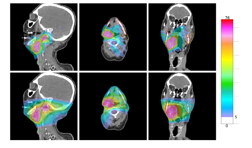
Figure 1: Plans created for case “H&N”. The group sparsity plan is shown in the top row, and the clinical plan is shown in the bottom row. Dose below 5 Gy is not shown.

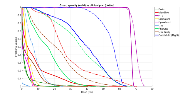
Figure 2: Dose-volume histogram for case “H&N”

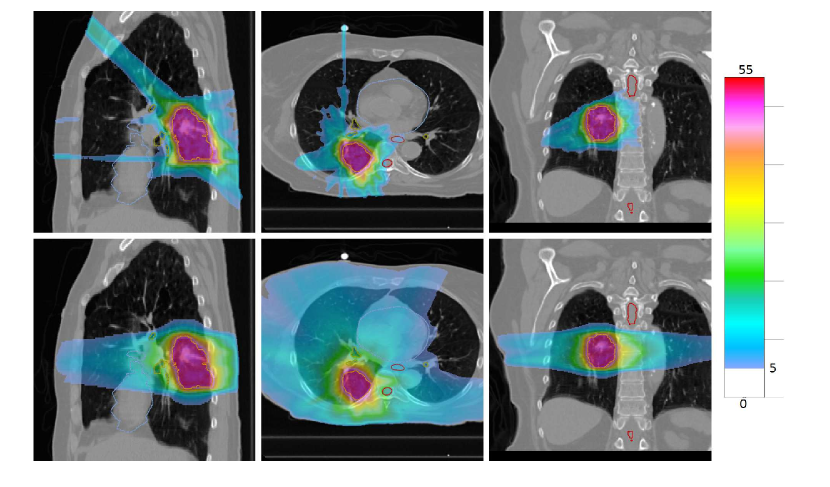
Figure 3: Plans created for case “LNG#1”. The group sparsity plan is shown in the top row, and the clinical plan is shown in the bottom row. Dose below 5 Gy is not shown.

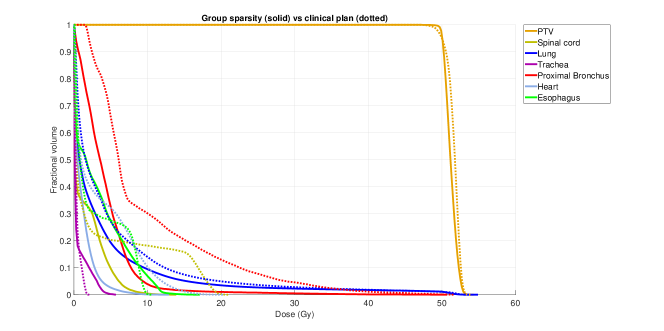
Figure 4: Dose-volume histogram for case “LNG#1”

TABLE II: PTV coverage metrics for several cases. Group sparsity results in black, clinical plan values in blue. The homogeneity index HI is defined as $\text{D}95/\text{D}5$.

Case	D95 (Gy)	D98 (Gy)	D99 (Gy)	$\text{D}_{\max}$	HI
H&N	66.0 [66.0]	65.7 [ 64.7]	65.3 [63.9]	68.6 [ 74.6]	.97 [.89]
LNG # 1	50.0 [50.0]	49.9 [49.4]	49.7 [49.0]	52.8 [53.0]	.95 [.95]
LNG # 2	48.0 [48.0]	47.7 [47.2]	47.5 [46.7]	51.3 [52.5]	.94 [.92]
PRT	40.0 [39.9]	39.7 [39.6]	39.5 [39.3]	42.2 [41.9]	.95 [.96]

TABLE III: OAR dose differences for several cases. For each case, the difference in mean dose $\text{D}_{\text{mean}}^{\text{GS}}-\text{D}_{\text{mean}}^{\text{clinic}}$ is computed for all OARs. (“GS” refers to the group sparsity treatment plan, and “clinic” refers to the clinical treatment plan.) The min, max, and average differences in mean dose are listed in columns 2 and 3. Likewise, the min, max, and average values of $\text{D}_{\text{max}}^{\text{GS}}-\text{D}_{\text{max}}^{\text{clinic}}$ are listed in columns 4 and 5.

		$\text{D}_{\text{mean}}^{\text{GS}}-\text{D}_{\text{mean}}^{\text{clinic}}$			$\text{D}_{\max}^{\text{GS}}-\text{D}_{\max}^{\text{clinic}}$
Case		average (Gy)	range (Gy)		average (Gy)	range (Gy)
H&N		-10.4	$[-21.1,-0.5]$		-15.0	$[-32.6,1.0]$
LNG#1		-1.8	$[-5.4,.30]$		-7.1	$[-23.6,2.2]$
LNG#2		-2.1	$[-4.6,.13]$		-5.2	$[-13.7,1.1]$
PRT		-3.1	$[-7.0,1.3]$		-1.2	$[-3.3,.02]$

Tables III and III show treatment plan quality metrics for the four cases listed in table I. The group sparsity plans show improvement in PTV D98 and PTV D99 for all cases, with PTV D98 increasing on average by .53 Gy and PTV D99 increasing on average by .78 Gy. PTV homogeneity improved from .89 to .97 for case “H&N” and remained constant or nearly constant for the other cases. For case “LNG#1”, the R50 values were $3.20$ for the group sparsity plan and $4.87$ for the clinical plan. For case “LNG#2”, the R50 values were $2.80$ for the group sparsity plan and $7.51$ for the clinical plan.

The average and range of OAR dose differences for each case are reported in table III. The group sparsity plans consistently show improvement over the clinical plans. Considering all OARs for all cases, mean OAR dose was reduced by 7.7% of the prescription dose, on average, and max OAR dose was reduced by 11% of the prescription dose, on average. Overall, considering doses washes, DVHs, and quality metrics, the dosimetric quality of the plans created using the group sparsity approach is superior to the dosimetric quality of the clinical plans.

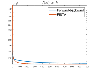
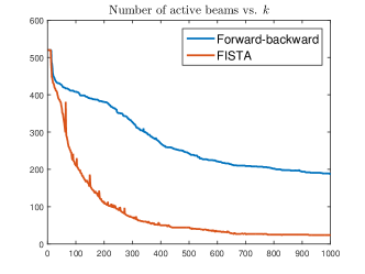
Figure 5: (a) Objective function value vs. iteration for both FISTA and the forward-backward method (which is the method used in [12]) for case “LNG#2”. Notice that after only 200 iterations FISTA has already done much better than 1000 iterations of the forward-backward method. (b) Number of active beams at each iteration for FISTA and the forward-backward method. After 1000 iterations, the solution computed by the forward-backward method still has $187$ active beams, and the method has not converged. Meanwhile, FISTA has converged to a solution with $24$ active beams (of which we kept the top $20$). The improved convergence rate of FISTA over the forward-backward method is the key to making the group sparsity approach practical for non-coplanar cases.

The FISTA runtimes for all cases are reported in table I. On average, the group sparsity plans took only 4.1 minutes to compute. We have observed that the number of iterations required for FISTA to converge is not very sensitive to the values of the weights appearing in the objective function. The convergence plot for case “LNG#2” in figure 5 shows the necessity of using an accelerated proximal gradient method. After 1000 iterations, the solution computed by the standard proximal gradient method (also known as the forward-backward method, which was the method used in [12]) still has $187$ active beams, and the method has not converged. Meanwhile, FISTA has converged to a solution with $24$ active beams (of which we kept the top $20$). The improved convergence rate of FISTA over the forward-backward method is the key to making the group sparsity approach practical for non-coplanar IMRT.

IV Discussion

The initial work [12] on group sparsity for beam orientation optimization was not practical for non-coplanar IMRT due to the slow convergence of the optimization algorithm. Without group sparsity, researchers developed greedy approaches in which fluence map optimization steps were interleaved with beam angle selection steps (with various heuristics available to select the next beam angle). In this study, we adopted an accelerated proximal gradient method (specifically, FISTA) to make the group sparsity approach practical for non-coplanar beam orientation optimization. The $O(1/k^{2})$ convergence rate of FISTA is a dramatic improvement on the $O(1/k)$ convergence rate of the standard proximal gradient method, also known as forward-backward method, which was used in [12]. We have observed that in beam orientation optimization problems for $4\pi$ non-coplanar radiotherapy, the standard proximal gradient method (also known as forward-backward method) does not converge to a group sparse solution in a reasonable amount of time; thus it is essential to use an accelerated algorithm. With the novel approach, we were able to solve large scale beam orientation optimization problems in a few minutes. Our Matlab implementation is able to select and optimize $20$ beams from $500-800$ candidate beams in about four minutes, producing treatment plans of dosimetric quality superior to that of plans which were used in a clinical setting. We improve considerably on the group sparsity results in [12], which was restricted to coplanar beams and reported runtimes of a few hours for coplanar head and neck cases with only 72 candidate beams. There are potential benefits from the improved computational speed beyond making beam orientation optimization practical for clinical adoption. The improvement also enables integration of beam orientation optimization with knowledge-based treatment planning and multi-criterion optimization where a large number of plans need to be created, allowing searching for optimal plans in an expanded solution space.

One of the challenges of promoting group sparsity is that the $\ell_{2,1}$-norm is nondifferentiable, so that we cannot use classical optimization algorithms such as quasi-Newton methods which assume the objective function is smooth. Proximal algorithms such as FISTA are very well suited for this type of large scale, nondifferentiable, constrained convex optimization problem. A key contribution of this paper is that we provide a closed-form expression (8) for the prox-operator of the function $g$ given by equation (6). (See appendix B for our derivation of this expression, which we have not found elsewhere in the literature.) Without the ability to evaluate this prox-operator efficiently, the large scale group sparsity problem would be intractable.

The computational time can be further improved to near real time. When solving problem (II-A) using FISTA, most of the computational time is spent on matrix-vector multiplications with the large sparse matrix $A$. Because these multiplications are embarrassingly parallel, our algorithm should benefit greatly from a multithreaded approach or a GPU implementation. Preliminary experiments suggest that these matrix-vector multiplications can be made over $100$ times faster when performed on a GPU. This is particularly important when a large number of plans need to be produced for Pareto or adaptive radiotherapy planning.

V Conclusions

By using an accelerated proximal gradient method, enabled by the prox-operator formula (8), we have obtained an orders of magnitude improvement on the runtimes reported in the initial work on beam orientation optimization by group sparsity [12], while improving on the dosimetric quality of plans that were used clinically. We have demonstrated that the group sparsity approach is fast and effective for non-coplanar beam orientation optimization.

Appendix A Proximal algorithms background

In this section we define the proximal operator and briefly review the proximal gradient method and FISTA. An accessible introduction to proximal algorithms can be found in [20]; see also [21, 22, 23].

A-A Proximal operator.

Let $f:\mathbb{R}^{n}\to\mathbb{R}\cup\{\infty\}$ be a closed (i.e., lower semi-continuous) convex function. The proximal operator (also known as “prox-operator”) of $f$, with parameter $t>0$, is defined by

$$\text{prox}_{tf}(x)=\operatorname*{arg\,min}_{u}\quad f(u)+\frac{1}{2t}\|u-x\|_{2}^{2}.$$ (9)

When we evaluate the proximal operator of $f$, it is as if we are trying to reduce the value of $f$ without straying too far from $x$. The parameter $t$ can be viewed as a “step size” that determines how much we’re penalized for moving away from $x$. Proximal algorithms are iterative optimization algorithms that require the evaluation of various prox-operators at each iteration. For many important convex penalty functions, the prox-operator has a simple closed-form expression and can be evaluated very efficiently, at a computational complexity that is linear in $n$.

A-B Proximal gradient method

One of the most fundamental proximal algorithms, the proximal gradient method (also known as the forward-backward method) solves optimization problems of the form

$$\operatorname*{\text{minimize}}\quad f(x)+g(x)$$ (10)

where $f$ and $g$ are closed convex functions and $f$ is differentiable with a Lipschitz continuous gradient. The proximal gradient method with line search is recorded in algorithm 1.

Algorithm 1 Proximal gradient method with line search

Initialize $x_{0}$ and $t_{0}>0$, select $0<r<1,s>1$

for $k=1,2,\ldots$ do

      $t\coloneqq s\,t_{k-1}$

      repeat

            $x\coloneqq\text{prox}_{tg}(x_{k-1}-t\nabla f(x_{k-1}))$

            break if $f(x)\leq f(x_{k-1})+\langle\nabla f(x_{k-1}),x-x_{k-1}\rangle+\frac{1}{2t}\|x-x_{k-1}\|_{2}^{2}$

            $t\coloneqq rt$       

      $t_{k}\coloneqq t$

      $x_{k}\coloneqq x$

end for

A-C Accelerated proximal gradient methods

A recent theme in convex optimization research has been the development of accelerated versions of the proximal gradient method [36, 37, 38, 39, 18, 40, 41, 42, 43, 44]. These methods are popular for medical image reconstruction problems, and they were applied to fluence map optimization problems (using the TFOCS software package [45]) in [46, 47]. In this paper, we focus on one particular accelerated method, FISTA [18] (short for “fast iterative shrinkage-thresholding algorithm”). FISTA is an accelerated version of the proximal gradient method for solving problem (10), where (as before) $f$ and $g$ are closed convex functions, and $f$ is differentiable with a Lipschitz continuous gradient. The FISTA with line search algorithm is recorded in algorithm 2. Note that the FISTA iteration is only a minor modification of the proximal gradient iteration. Yet, FISTA converges at a rate of $O(1/k^{2})$ (where $k$ is the iteration number), whereas the proximal gradient iteration only converges at a rate of $O(1/k)$. FISTA’s convergence rate of $O(1/k^{2})$ is in some sense optimal for a first-order method [36]. Although we focus on FISTA in this paper, it is not the only method that achieves this optimal $O(1/k^{2})$ convergence rate [37, 39, 36, 44].

Algorithm 2 FISTA with line search

Initialize $x_{0}$ and $t_{0}>0$, set $v_{0}\coloneqq x_{0}$, select $0<r<1$, $s>1$

for $k=1,2,\ldots$ do

      $t\coloneqq s\,t_{k-1}$

      repeat

            $\theta\coloneqq\begin{cases}1&\quad\text{if }k=1\\ \text{positive root of }t_{k-1}\theta^{2}=t\theta_{k-1}^{2}(1-\theta)&\quad\text{if }k>1\end{cases}$

            $y\coloneqq(1-\theta)x_{k-1}+\theta v_{k-1}$

            $x\coloneqq\text{prox}_{tg}(y-t\nabla f(y))$

            break if $f(x)\leq f(y)+\langle\nabla f(y),x-y\rangle+\frac{1}{2t}\|x-y\|_{2}^{2}$

            $t\coloneqq rt$       

      $t_{k}\coloneqq t$

      $\theta_{k}\coloneqq\theta$

      $x_{k}\coloneqq x$

      $v_{k}\coloneqq x_{k-1}+\frac{1}{\theta_{k}}(x_{k}-x_{k-1})$

end for

Appendix B Prox-operator calculation

Here we derive a formula for the prox-operator of the function

$$f(x)=\begin{cases}\|x\|_{2}&\quad\text{if }x\geq 0\\ \infty&\quad\text{otherwise}.\end{cases}$$

(The inequality $x\geq 0$ is interpreted componentwise.) Let $t>0$. To evaluate $\text{prox}_{tf}(\hat{x})$, we must find the minimizer for the problem

$$\operatorname*{\text{minimize}}_{x} \quad\|x\|_{2}+\frac{1}{2t}\|x-\hat{x}\|_{2}^{2}$$ (11)

subject to $$\quad x\geq 0.$$

First note that if $\hat{x}_{i}\leq 0$ then there is no benefit from taking $x_{i}$ to be positive. If $x_{i}$ were positive, then both terms in the objective function could be reduced just by setting $x_{i}=0$.

It remains only to select values for the other components of $x$. This is a smaller optimization problem, with one unknown for each positive component of $\hat{x}$. The negative components of $\hat{x}$ are irrelevant to the solution of this reduced problem. Thus, we would still arrive at the same final answer if the negative components of $\hat{x}$ were set equal to $0$ at the very beginning.

In other words, problem (11) is equivalent to the problem

$$\operatorname*{\text{minimize}}_{x} \quad\|x\|_{2}+\frac{1}{2t}\|x-\max(\hat{x},0)\|_{2}^{2}$$

subject to $$\quad x\geq 0,$$

which in turn is equivalent to the problem

$$\operatorname*{\text{minimize}}_{x} \quad\|x\|_{2}+\frac{1}{2t}\|x-\max(\hat{x},0)\|_{2}^{2}$$

(because there would be no benefit from taking any components of $x$ to be negative). This shows that

$$\text{prox}_{tf}(\hat{x})=\text{prox}_{t\|\cdot\|_{2}}(\max(\hat{x},0)).$$ (12)

As mentioned previously, a standard formula for the prox-operator of the $\ell_{2}$-norm is

$$\text{prox}_{t\|\cdot\|_{2}}(y)=y-Py,$$

where $Py$ is the projection of $y$ onto the $\ell_{2}$-norm ball of radius $t$.

References

- [1] K. Woods, D. Nguyen, A. Tran, V. Yu, M. Cao, T. Niu, P. Lee, and K. Sheng, “Viability of non-coplanar VMAT for liver SBRT as compared to coplanar VMAT and beam orientation optimized 4 IMRT,” Advances in Radiation Oncology, 2016.
- [2] H. Romeijn, R. Ahuja, J. Dempsey, and A. Kumar, “A column generation approach to radiation therapy treatment planning using aperture modulation,” SIAM Journal on Optimization, vol. 15, no. 3, pp. 838–862, 2005.
- [3] S. Breedveld, P. Storchi, P. Voet, and B. Heijmen, “iCycle: Integrated, multicriterial beam angle, and profile optimization for generation of coplanar and noncoplanar IMRT plans,” Medical Physics, vol. 39, no. 2, pp. 951–963, 2012.
- [4] G. Lim, J. Choi, and R. Mohan, “Iterative solution methods for beam angle and fluence map optimization in intensity modulated radiation therapy planning,” OR Spectrum, vol. 30, no. 2, pp. 289–309, 2008.
- [5] D. Bertsimas, V. Cacchiani, D. Craft, and O. Nohadani, “A hybrid approach to beam angle optimization in intensity-modulated radiation therapy,” Computers & Operations Research, vol. 40, no. 9, pp. 2187–2197, 2013.
- [6] H. Yarmand and D. Craft, “Two effective heuristics for beam angle optimization in radiation therapy,” arXiv preprint arXiv:1305.4959, 2013.
- [7] H. Rocha, J. Dias, B. Ferreira, and M. do Carmo Lopes, “Does beam angle optimization really matter for intensity-modulated radiation therapy?” in Computational Science and Its Applications–ICCSA 2015. Springer, 2015, pp. 522–533.
- [8] M. Bangert and J. Unkelbach, “Accelerated iterative beam angle selection in IMRT,” Medical Physics, vol. 43, no. 3, pp. 1073–1082, 2016.
- [9] P. Dong, P. Lee, D. Ruan, T. Long, E. Romeijn, Y. Yang, D. Low, P. Kupelian, and K. Sheng, “4 non-coplanar liver SBRT: A novel delivery technique,” International Journal of Radiation Oncology* Biology* Physics, vol. 85, no. 5, pp. 1360–1366, 2013.
- [10] P. Dong, D. Nguyen, D. Ruan, C. King, T. Long, E. Romeijn, D. A. Low, P. Kupelian, M. Steinberg, Y. Yang, and K. Sheng, “Feasibility of prostate robotic radiation therapy on conventional C-arm linacs,” Practical Radiation Oncology, vol. 4, no. 4, pp. 254–260, 2014.
- [11] P. Dong, P. Lee, D. Ruan, T. Long, E. Romeijn, D. A. Low, P. Kupelian, J. Abraham, Y. Yang, and K. Sheng, “4 non-coplanar stereotactic body radiation therapy for centrally located or larger lung tumors,” International Journal of Radiation Oncology* Biology* Physics, vol. 86, no. 3, pp. 407–413, 2013.
- [12] X. Jia, C. Men, Y. Lou, and S. Jiang, “Beam orientation optimization for intensity modulated radiation therapy using adaptive -minimization,” Physics in Medicine and Biology, vol. 56, no. 19, 2011.
- [13] F. Bach, R. Jenatton, J. Mairal, and G. Obozinski, “Optimization with sparsity-inducing penalties,” Foundations and Trends® in Machine Learning, vol. 4, no. 1, pp. 1–106, 2012.
- [14] N. Simon, J. Friedman, T. Hastie, and R. Tibshirani, “A sparse-group lasso,” Journal of Computational and Graphical Statistics, vol. 22, no. 2, pp. 231–245, 2013.
- [15] L. Meier, S. Van De Geer, and P. Bühlmann, “The group lasso for logistic regression,” Journal of the Royal Statistical Society: Series B (Statistical Methodology), vol. 70, no. 1, pp. 53–71, 2008.
- [16] F. Bach, “Consistency of the group lasso and multiple kernel learning,” The Journal of Machine Learning Research, vol. 9, pp. 1179–1225, 2008.
- [17] J. Huang and T. Zhang, “The benefit of group sparsity,” The Annals of Statistics, vol. 38, no. 4, pp. 1978–2004, 2010.
- [18] A. Beck and M. Teboulle, “A fast iterative shrinkage-thresholding algorithm for linear inverse problems,” SIAM Journal on Imaging Sciences, vol. 2, no. 1, pp. 183–202, 2009.
- [19] D. O’Connor, Y. Voronenko, D. Nguyen, W. Yin, and K. Sheng, “4 non-coplanar IMRT beam angle selection by convex optimization with group sparsity penalty,” Medical Physics, vol. 43, no. 6, pp. 3895–3895, 2016.
- [20] N. Parikh and S. Boyd, “Proximal algorithms,” Foundations and Trends in Optimization, vol. 1, no. 3, pp. 123–231, 2013.
- [21] A. Chambolle and T. Pock, “An introduction to continuous optimization for imaging,” Acta Numerica, vol. 25, pp. 161–319, 2016.
- [22] L. Vandenberghe, “UCLA course EE 236c: Optimization methods for large-scale systems,” Lecture notes.
- [23] P. L. Combettes and J.-C. Pesquet, “Proximal splitting methods in signal processing,” in Fixed-point algorithms for inverse problems in science and engineering. Springer, 2011, pp. 185–212.
- [24] R. Glowinski and A. Marroco, “Sur l’approximation, par éléments finis d’ordre un, et la résolution, par pénalisation-dualité d’une classe de problèmes de dirichlet non linéaires,” Revue française d’automatique, informatique, recherche opérationnelle. Analyse numérique, vol. 9, no. 2, pp. 41–76, 1975.
- [25] D. Gabay and B. Mercier, “A dual algorithm for the solution of nonlinear variational problems via finite element approximation,” Computers & Mathematics with Applications, vol. 2, no. 1, pp. 17–40, 1976.
- [26] S. Boyd, N. Parikh, E. Chu, B. Peleato, and J. Eckstein, “Distributed optimization and statistical learning via the alternating direction method of multipliers,” Foundations and Trends® in Machine Learning, vol. 3, no. 1, pp. 1–122, 2011.
- [27] A. Chambolle and T. Pock, “A first-order primal-dual algorithm for convex problems with applications to imaging,” Journal of Mathematical Imaging and Vision, vol. 40, no. 1, pp. 120–145, 2011.
- [28] T. Pock, A. Chambolle, D. Cremers, and H. Bischof, “A convex relaxation approach for computing minimal partitions,” in Computer Vision and Pattern Recognition, 2009. CVPR 2009. IEEE Conference on. IEEE, 2009, pp. 810–817.
- [29] N. Parikh and S. Boyd, “Block splitting for distributed optimization,” Mathematical Programming Computation, vol. 6, no. 1, pp. 77–102, 2014.
- [30] L. Ghaoui, V. Viallon, and T. Rabbani, “Safe feature elimination for the lasso and sparse supervised learning problems,” arXiv preprint arXiv:1009.4219, 2010.
- [31] R. Tibshirani, J. Bien, J. Friedman, T. Hastie, N. Simon, J. Taylor, and R. Tibshirani, “Strong rules for discarding predictors in lasso-type problems,” Journal of the Royal Statistical Society: Series B (Statistical Methodology), vol. 74, no. 2, pp. 245–266, 2012.
- [32] J. Friedman, T. Hastie, and R. Tibshirani, “Glmnet: Lasso and elastic-net regularized generalized linear models,” R package version, vol. 1, 2009.
- [33] V. Yu, A. Tran, D. Nguyen, M. Cao, D. Ruan, D. Low, and K. Sheng, “The development and verification of a highly accurate collision prediction model for automated noncoplanar plan delivery,” Medical Physics, vol. 42, no. 11, pp. 6457–6467, 2015.
- [34] J. Neylon, K. Sheng, V. Yu, Q. Chen, D. Low, P. Kupelian, and A. Santhanam, “A nonvoxel-based dose convolution/superposition algorithm optimized for scalable GPU architectures,” Medical Physics, vol. 41, no. 10, 2014.
- [35] V. Grégoire and T. Mackie, “State of the art on dose prescription, reporting and recording in intensity-modulated radiation therapy (icru report no. 83),” Cancer/Radiothérapie, vol. 15, no. 6, pp. 555–559, 2011.
- [36] Y. Nesterov, Introductory lectures on convex optimization. Springer Science & Business Media, 2004, vol. 87.
- [37] P. Tseng, “On accelerated proximal gradient methods for convex-concave optimization,” SIAM J. Optimization, 2008.
- [38] Y. Nesterov, “A method of solving a convex programming problem with convergence rate ,” in Soviet Mathematics Doklady, vol. 27, no. 2, 1983, pp. 372–376.
- [39] ——, “Smooth minimization of non-smooth functions,” Mathematical Programming, vol. 103, no. 1, pp. 127–152, 2005.
- [40] A. Beck and M. Teboulle, “Gradient-based algorithms with applications to signal recovery,” Convex Optimization in Signal Processing and Communications, 2009.
- [41] ——, “Fast gradient-based algorithms for constrained total variation image denoising and deblurring problems,” Image Processing, IEEE Transactions on, vol. 18, no. 11, pp. 2419–2434, 2009.
- [42] K. Scheinberg, D. Goldfarb, and X. Bai, “Fast first-order methods for composite convex optimization with backtracking,” Foundations of Computational Mathematics, vol. 14, no. 3, pp. 389–417, 2014.
- [43] Y. Nesterov, “Gradient methods for minimizing composite objective function,” 2007.
- [44] S. Becker, J. Bobin, and E. J. Candès, “NESTA: A fast and accurate first-order method for sparse recovery,” SIAM Journal on Imaging Sciences, vol. 4, no. 1, pp. 1–39, 2011.
- [45] S. Becker, E. Candès, and M. Grant, “Templates for convex cone problems with applications to sparse signal recovery,” Mathematical Programming Computation, vol. 3, no. 3, pp. 165–218, 2011.
- [46] H. Kim, R. Li, R. Lee, T. Goldstein, S. Boyd, E. Candes, and L. Xing, “Dose optimization with first-order total-variation minimization for dense angularly sampled and sparse intensity modulated radiation therapy (dassim-rt),” Medical Physics, vol. 39, no. 7, pp. 4316–4327, 2012.
- [47] H. Kim, T. Suh, R. Lee, L. Xing, and R. Li, “Efficient IMRT inverse planning with a new -solver: template for first-order conic solver,” Physics in Medicine and Biology, vol. 57, no. 13, p. 4139, 2012.