Uniform Consistency in Stochastic Block Model with Continuous Community Label

Abstract

Bickel and Chen, (2009) developed a general framework to establish consistency of community detection in stochastic block model (SBM). In most applications of this framework, the community label is discrete. For example, in (Bickel and Chen,, 2009; Zhao et al.,, 2012) the degree corrected SBM is assumed to have a discrete degree parameter. In this paper, we generalize the method of Bickel and Chen, (2009) to give consistency analysis of maximum likelihood estimator (MLE) in SBM with continuous community label. We show that there is a standard procedure to transform the $||\cdot||_{2}$ error bound to the uniform error bound $||\cdot||_{\infty}$. We demonstrate the application of our general results by proving the uniform consistency (strong consistency) of the MLE in the exponential network model with interaction effect. As far as we know, this is yet unknown. Unfortunately, in the continuous parameter case, the condition ensuring uniform consistency we obtained is much stronger than that in the discrete parameter case, namely $n\mu_{n}^{5}/(\log n)^{8}\rightarrow\infty$ versus $n\mu_{n}/\log n\rightarrow\infty$. Where $n\mu_{n}$ represents the average degree of the network. But continuous is the limit of discrete. So it is not surprising as we show that by discretizing the community label space into sufficiently small (but not too small) pieces and applying the MLE on the discretized community label space, uniform consistency holds under almost the same condition as in discrete community label space. Such a phenomenon is surprising since the discretization does not depend on the data or the model. This reminds us of the thresholding method. Another purpose of this paper is to investigate whether the uniform consistency condition in the continuous community label case is necessarily stronger than that in the discrete parameter case. We did not find a numerical example confirming this. However, a numerical experiment shows that the uniform error bound and the mean square error bound of the MLE, approximated by the gradient decent algorithm, are not reduced by strengthening the stopping criterion. This coincides with the result that running the MLE on a subset of the parameter space reduces the uniform error bound.

Key words: stochastic block model, parameter estimation, asymptotic theory

1 Introduction

SBM is one of the most popular network model, not only because of its simplicity, but also for the following reasons. First, it well fits a lot of real world data in the following fields,social network (Holland and Leinhardt,, 1981; Newman et al.,, 2002; Robins et al.,, 2009) (notably, Holland and Leinhardt, (1981) first proposed SBM), biology Rohe et al., (2011), gene regulatory network (Schlitt and Brazma,, 2007; Pritchard et al.,, 2000), image processing (Shi and Malik,, 2000; Sonka et al.,, 2008). Second, the model is a nice tool to investigate community detection algorithms from the theoretical perspective. (Dyer and Frieze,, 1989; Jerrum and Sorkin,, 1998; Condon and Karp,, 2001) are early works in this stream. Although their focus is the algorithmic aspects of the min-bisection problem. Later a vast amount of research is carried out to study and compare the performance of various community detection algorithms on SBM. Roughly speaking, these algorithms can be divided into the following categories. Modularity algorithm (Newman and Girvan,, 2004) etc, likelihood algorithm (Bickel and Chen,, 2009; Choi et al.,, 2012; Amini et al.,, 2013; Celisse et al.,, 2012) etc, and most importantly, spectral algorithm (Chatterjee et al.,, 2011; Balakrishnan et al.,, 2011; Jin,, 2015; Sarkar and Bickel,, 2013; Krzakala et al.,, 2013) etc.

Notably, Bickel and Chen, (2009) provided a general framework to check the consistency of community detection. It was further extended by (Zhao et al.,, 2012) to establish consistency of many community detection algorithms in more general models. These algorithms include maximum likelihood estimation and various modularity methods. The technique is mainly based on finite covering method and concentration inequality. This approach is also employed to establish consistency of spectral clustering (Lei et al.,, 2015). Most of works concerning consistency of parameter estimation in SBM focused on discrete community label (finitely many blocks). A few exceptions include: (Yan et al.,, 2015) dealing with exponential network model; (Xu et al.,, 2014),(Jog and Loh,, 2015) dealing with SBM with edge label (edge weight); and (Jin et al.,, 2016) studying mixed membership. The general picture is still lack. Whether uniform consistency and weak consistency holds in SBM with continuous membership under similar condition as that in discrete membership case? On the surface, continuous community label space is simply the limit of discrete community label space. However, the uniform consistency (strong consistency) condition we obtained in continuous community label space is stronger than that in discrete community label space. It is not clear if such gap is inevitable.

1.1 Outline

The paper is organized as follows. We define the SBM in section 1.2 and introduce notations in section 1.3. In section 2 we define uniform consistency and weak consistency. In section 2.1 we first give the condition of weak consistency and uniform consistency for the exponential network model. As in (Bickel and Chen,, 2009; Zhao et al.,, 2012), the condition is about the density (average connection probability) of the network. Then in section 2.1 we present results for weak consistency and uniform consistency in the general SBM. The condition for weak consistency is slightly stronger than that in the discrete community label space. However, the uniform consistency condition we obtained is much stronger than that in the discrete community label space in (Bickel and Chen,, 2009; Zhao et al.,, 2012). We are not clear if the condition is necessarily stronger. However, continuous is the limit of discrete. Therefore, it is not surprise as we show in section 2.3 that by discretizing the community label space and applying the MLE on the discretized community label space, the condition ensuring uniform consistency is almost the same as that in discrete community label space in (Bickel and Chen,, 2009; Zhao et al.,, 2012). In section 3.1, we present our simulation results. They show that our theoretical results are possibly far from the truth. First, we run gradient decent algorithm for the MLE in the exponential network model. The results indicate that the error of the MLE is asymptotically normal and uniformly consistent. We have not found an example verifying that the condition ensuring uniform consistency in continuous community label space is necessarily stronger than that in the discretized community label space. But our second experiment shows that the performance of the gradient decent algorithm, measured by the uniform error bound, can be reduced by relaxing the stopping criterion. This is an evidence that the MLE can be overfitting.

1.2 Model description

A network of size $n$ is determined by $n(n-1)/2$ variables $Y_{ij}\in\mathcal{S},i<j\leq n$. $Y_{ij}$ represents the connection type between node $i,j$. For an undirected network $\mathcal{S}=\{0,1\}$; for a directed network $\mathcal{S}=\{0,1\}^{2}$. More complicated state space is possible (Lelarge et al.,, 2015). In all these settings, there exists an element $\mathbf{0}\in\mathcal{S}$ indicating ”no connection”. In a stochastic block model (SBM), each node $i$ is assigned a latent type $\boldsymbol{\eta}_{i}$. Conditional on $\boldsymbol{\eta}$, $Y_{ij}$ are mutually independent, and $\mathbb{P}(Y_{ij}=y|\boldsymbol{\eta})=\Theta_{ij}(y;\boldsymbol{\eta}_{i},\boldsymbol{\eta}_{j},\boldsymbol{\rho},\mu_{n})$ where $\boldsymbol{\rho}$ is the model parameter and $n\mu_{n}$ reflects the order of average degree. In a typical SBM consisting of $K$ communities, $\boldsymbol{\eta}_{i}\in\{1,2,\cdots,K\}$ represents the community label of $i$ and $\boldsymbol{\rho}$ is a $K\times K$ matrix characterizing the between community connection probability. In this paper, we study the case where $\boldsymbol{\eta}_{i}$ can be continuous variable. In many settings, the network is somewhat sparse, which requires $\Theta_{ij}$ to scale with the network size $n$. We set

$$\Theta_{ij}(y;\boldsymbol{\eta}_{i},\boldsymbol{\eta}_{j},\boldsymbol{\rho},\mu_{n})=\mu_{n}f(y;\boldsymbol{\eta}_{i},\boldsymbol{\eta}_{j},\boldsymbol{\rho})\text{ if }y\neq\mathbf{0};$$ (1)

$$\Theta_{ij}(\mathbf{0};\boldsymbol{\eta}_{i},\boldsymbol{\eta}_{j},\boldsymbol{\rho},\mu_{n})=1-\sum\limits_{y}\Theta_{ij}(y;\boldsymbol{\eta}_{i},\boldsymbol{\eta}_{j},\boldsymbol{\rho},\mu_{n}),$$

where $f$ is a fixed function. Model (1) clearly includes the traditional SBM (finitely many communities), degree-corrected SBM and a special case of the exponential network model (see section 2.1 or (Yan et al.,, 2015)). In many settings, there is a model identification problem concerning $\mu_{n}$. We restrict on two settings of $\mu_{n}$:

• $n\mu_{n}$ is the average ”degree”, i.e., $\mu_{n}=\mathbb{P}(Y_{ij}\neq\mathbf{0})$;

• $\mu_{n}$ is known and represents a level of density of the network say, $\mu_{n}=\frac{\log n}{n}$, $\mu_{n}=1$ etc.

In both cases we write $\overline{\mu}_{n}$ for the estimator of $\mu_{n}$. There may also be a model identification problem concerning $\boldsymbol{\eta},\boldsymbol{\rho}$. For example, in the SBM with finitely many blocks, a permutation of community labels gives the same model. For two parameters $\boldsymbol{\eta},\boldsymbol{\rho}$ and $\boldsymbol{\eta}^{\prime},\boldsymbol{\rho}^{\prime}$, we write $\boldsymbol{\eta},\boldsymbol{\rho}\cong\boldsymbol{\eta}^{\prime},\boldsymbol{\rho}^{\prime}$ if for all $i,j\leq n$, $\Theta_{ij}(\cdot;\boldsymbol{\eta}_{i},\boldsymbol{\eta}_{j},\boldsymbol{\rho},\mu_{n})=\Theta_{ij}(\cdot;\boldsymbol{\eta}_{i}^{\prime},\boldsymbol{\eta}_{j}^{\prime},\boldsymbol{\rho}^{\prime},\mu_{n})$. We say a parameter $\boldsymbol{\eta},\boldsymbol{\rho}$ is true iff $\boldsymbol{\eta},\boldsymbol{\rho}\cong\boldsymbol{\eta}^{*},\boldsymbol{\rho}^{*}$. Where $\boldsymbol{\eta}^{*},\boldsymbol{\rho}^{*}$ are realized true parameter. In the following text, we denote by $\boldsymbol{\eta}^{*},\boldsymbol{\rho}^{*},\mu_{n}^{*}$ any true values of $\boldsymbol{\eta},\boldsymbol{\rho},\mu_{n}$. Two major tasks in network data analysis are community detection— estimating $\boldsymbol{\eta}$, and parameter estimation —estimating $\boldsymbol{\rho}$. We call them both parameter estimation since we regard $\boldsymbol{\eta}$ also as parameters. Clearly, the log likelihood function is,

$$\ell(\mathbf{Y};\boldsymbol{\eta},\boldsymbol{\rho},\mu_{n})=\sum\limits_{i<j\leq n}\log\Theta_{ij}(Y_{ij};\boldsymbol{\eta}_{i},\boldsymbol{\eta}_{j},\boldsymbol{\rho},\mu_{n}).$$

We define the maximum likelihood estimator, namely $\hat{\boldsymbol{\eta}},\hat{\boldsymbol{\rho}}$, to be the maximizer of $\ell(\mathbf{Y};\boldsymbol{\eta},\boldsymbol{\rho},\overline{\mu}_{n})$.

1.3 Notations

Let $\mathbf{Y}$ denote the vector $(\cdots,Y_{ij},\cdots)$, $i<j\leq n$, $\mathbf{Y}_{i}$ denote the vector $(Y_{i1},Y_{i2},\cdots,Y_{in})$. For a random variable $W$ with distribution $p_{\theta}$, write $\operatorname{E}_{\theta^{\prime}}(W)$ for $\operatorname{E}_{W\sim p_{\theta^{\prime}}}(W)$; write $\operatorname{E}_{W}(g(W))$ ($Var_{W}(g(W))$) to denote the expectation (variation) with respect to $W$ (when no ambiguity is made the subscript is omitted). For any vector $\mathbf{v}\in\mathbb{R}^{n}$, let $\mathbf{v}_{-i}$ denote the vector $(v_{1},\cdots,v_{i-1},v_{i+1},\cdots,v_{n})$; abusing the notation, for any real $x$ write $\mathbf{v}+x$ for $(v_{1}+x,\cdots,v_{n}+x)$; for a sequence $X\in\{0,1\}^{n}$, write $||\mathbf{v}||_{p,X}$ for $(\sum\limits_{i:X(i)=1}|v_{i}|^{p})^{\frac{1}{p}}$.

Let

$$\ell_{i}(\mathbf{Y}_{i};\boldsymbol{\eta},\boldsymbol{\rho},\mu_{n})=\sum\limits_{j\leq n}\log\Theta_{ij}(Y_{ij};\boldsymbol{\eta}_{i},\boldsymbol{\eta}_{j},\boldsymbol{\rho},\mu_{n}),$$ (2)

$$\ell_{ij}(Y_{ij};\boldsymbol{\eta},\boldsymbol{\rho},\mu_{n})=\log\Theta_{ij}(Y_{ij};\boldsymbol{\eta}_{i},\boldsymbol{\eta}_{j},\boldsymbol{\rho},\mu_{n}).$$

We write $\hat{\boldsymbol{\rho}},\hat{\boldsymbol{\eta}}$ for the MLE of the parameters if not claimed otherwise.

For two sequences $a_{n},b_{n}$, we write $a_{n}=\Omega(b_{n})$ iff $b_{n}=O(a_{n})$; $a_{n}=\Theta(b_{n})$ iff $a_{n}=O(b_{n}),b_{n}=O(a_{n})$. For two sequences of function $a_{n}(x),b_{n}(x)$ we say $a_{n}(x)=O(b_{n}(x))$ uniformly in $x$ iff there exists $C$ such that $a_{n}(x)\leq Cb_{n}(x)$ for all $x$, and similarly for $\Omega,O_{p},o_{p}$ notation.

2 Main Result

In the finite block setting, there are two main concepts of consistency for community detection, weak consistency and uniform consistency (strong consistency). The weak consistency means that with large probability, the estimator of latent types is mostly correct. The uniform consistency means that with large probability, the estimator of latent types is all correct. In the continuous parameter setting, the appropriate measure for weak and uniform consistency are $||\cdot||_{p}$ norm and $||\cdot||_{\infty}$ norm where $0<p<\infty$. In particular, we adopt $||\cdot||_{2}$ as the weak consistency measure. i.e., $\hat{\boldsymbol{\eta}}$ is weak consistent iff $\inf\limits_{\boldsymbol{\eta},\boldsymbol{\rho}\text{ true}}||\boldsymbol{\hat{\eta}}-\boldsymbol{\eta}||_{2}\xrightarrow{p}0$; $\hat{\boldsymbol{\eta}}$ is uniform consistent iff $\inf\limits_{\boldsymbol{\eta},\boldsymbol{\rho}\text{ true}}||\boldsymbol{\hat{\eta}}-\boldsymbol{\eta}||_{\infty}\xrightarrow{p}0$

2.1 Consistency in exponential network model

For a directed network model write $a_{ij}=1$ to indicate the existence of an edge from $i$ to $j$. The exponential network model with interaction effect we study is a directed network model with each node’s latent type being $\alpha_{i},\beta_{i}\in\mathbb{R}$. The distribution of $Y_{ij}=(a_{ij},a_{ji})$, given $\alpha_{i},\beta_{i},i\leq n,\rho\in\mathbb{R}$, is as follows:

$$g(a_{ij},a_{ji};\alpha_{i},\beta_{i},\alpha_{j},\beta_{j},\rho)$$ (3)

$$= \frac{1}{Z(\alpha_{i},\beta_{i},\alpha_{j},\beta_{j},\rho)}\exp\big{\{}\big{[}(\alpha_{i}+\beta_{j})a_{ij}+(\beta_{i}+\alpha_{j})a_{ji}\ \big{]}+\rho a_{ij}a_{ji}\big{\}}.$$

In this model we set $\mu_{n}^{*}=1$. There is clearly a model identification problem. The models defined by $(\boldsymbol{\alpha},\boldsymbol{\beta},\rho)$ and $(\boldsymbol{\alpha}-x,\boldsymbol{\beta}+x,\rho)$ are identical for all $x\in\mathbb{R}$. Thus, without loss of generality, we assume $\alpha_{1}^{*}=\hat{\alpha}_{1}=0$. For the exponential model without interaction effect (i.e., $\rho=0$), Yan et al., (2015) verified the uniform consistency and Yan et al., (2016) even proved the asymptotic normality of the MLE by analysing the inverse of the sample covariance matrix. The following theorem 2.1 verifies the ”weak consistency” of the MLE in model (3).

Theorem 2.1.

Suppose $\alpha_{i}^{*},\beta_{i}^{*},\rho^{*}$ are uniformly bounded within $[-B,B]$. Set $\Delta\alpha=\frac{1}{n}\sum\limits_{i\leq n}(\hat{\alpha}_{i}-\alpha_{i}^{*}),\Delta\beta=\frac{1}{n}\sum\limits_{i\leq n}(\hat{\beta}_{i}-\beta_{i}^{*})$. Then we have:

• $(\hat{\rho}-\rho)^{2}=O_{p}(n^{-\frac{1}{2}}(\log n)^{2})$;

• $(\Delta\alpha+\Delta\beta)^{2}=O_{p}(n^{-\frac{1}{2}}(\log n)^{2});$

• $||\boldsymbol{\hat{\alpha}}-\boldsymbol{\alpha}^{*}-\Delta\alpha||_{2}^{2}+||\boldsymbol{\hat{\beta}}-\boldsymbol{\beta}^{*}-\Delta\beta||_{2}^{2}=O_{p}(n^{\frac{1}{2}}(\log n)^{2}).$

As we show in the proof in appendix, uniform consistency can be obtained from the ”weak consistency”.

Theorem 2.2.

Suppose $\alpha_{i}^{*},\beta_{i}^{*},\rho^{*}$ are uniformly bounded within $[-B,B]$. Then we have:

$$||\hat{\boldsymbol{\alpha}}-\boldsymbol{\alpha}^{*}||_{\infty}+||\hat{\boldsymbol{\beta}}-\boldsymbol{\beta}^{*}||_{\infty}=O_{p}(n^{-\frac{1}{8}}\sqrt{\log n}).$$

Both theorem 2.1,2.2 are conclusions of more general theorems given in subsection 2.2.

2.2 A general result on uniform consistency

We make the following regular and bounding assumption on $f$ and $\mathcal{B}_{i}$.

Assumption 2.3.

1. There exists a compact subset of $\mathbb{R}^{d}$, $\mathcal{B}$, with $\mathcal{B}_{i}\subseteq\mathcal{B}$ for all $i\leq n$ and $\boldsymbol{\rho}\in\mathcal{B}$.

2. For some constant $0<c\leq C$, $c\leq f(y;\boldsymbol{\eta}_{i},\boldsymbol{\eta}_{j},\boldsymbol{\rho})\leq C$ for all $\boldsymbol{\eta}_{i}\in\mathcal{B}_{i},\boldsymbol{\eta}_{j}\in\mathcal{B}_{j},\boldsymbol{\rho}\in\mathcal{B},y\in\mathcal{S}-\mathbf{0}$.

3. There exists a constant $C_{3}$ such that for any $\boldsymbol{\eta}^{\prime},\boldsymbol{\rho}^{\prime}$, $\boldsymbol{\eta}^{\prime\prime},\boldsymbol{\rho}^{\prime\prime}$:

   $$\sum\limits_{i<j\leq n}||f(\cdot;\boldsymbol{\eta}_{i}^{\prime},\boldsymbol{\eta}_{j}^{\prime},\boldsymbol{\rho}^{\prime})-f(\cdot;\boldsymbol{\eta}_{i}^{\prime\prime},\boldsymbol{\eta}_{j}^{\prime\prime},\boldsymbol{\rho}^{\prime\prime})||_{2}^{2}\geq C_{3}\cdot\inf\limits_{\boldsymbol{\eta},\boldsymbol{\rho\cong\boldsymbol{\eta}^{\prime\prime},\boldsymbol{\rho}^{\prime\prime}}}\big{\{}\ ||\boldsymbol{\eta}^{\prime}-\boldsymbol{\eta}||_{2}^{2}+n||\boldsymbol{\rho}^{\prime}-\boldsymbol{\rho}||_{2}^{2}\ \big{\}}.$$

4. For some constant $C_{1}>0$, $\big{|}\big{|}\frac{\partial f(y,\boldsymbol{\eta}_{i},\boldsymbol{\eta}_{j},\boldsymbol{\rho})}{\partial\boldsymbol{\eta}_{i}}\big{|}\big{|}_{2},\big{|}\big{|}\frac{\partial f(y,\boldsymbol{\eta}_{i},\boldsymbol{\eta}_{j},\boldsymbol{\rho})}{\partial\boldsymbol{\eta}_{j}}\big{|}\big{|}_{2}$, $\big{|}\big{|}\frac{\partial f(y,\boldsymbol{\eta}_{i},\boldsymbol{\eta}_{j},\boldsymbol{\rho})}{\partial\boldsymbol{\rho}}\big{|}\big{|}_{2}$ , $\big{|}\big{|}\frac{\partial^{2}f(y,\boldsymbol{\eta}_{i},\boldsymbol{\eta}_{j},\boldsymbol{\rho})}{\partial\boldsymbol{\eta}_{i}^{2}}\big{|}\big{|}_{2}$, $\big{|}\big{|}\frac{\partial^{2}f(y,\boldsymbol{\eta}_{i},\boldsymbol{\eta}_{j},\boldsymbol{\rho})}{\partial\boldsymbol{\eta}_{j}^{2}}\big{|}\big{|}_{2}$, $\big{|}\big{|}\frac{\partial^{2}f(y,\boldsymbol{\eta}_{i},\boldsymbol{\eta}_{j},\boldsymbol{\rho})}{\partial\boldsymbol{\rho}^{2}}\big{|}\big{|}_{2}<C_{1}$ for all $\boldsymbol{\eta}_{i}\in\mathcal{B}_{i},\boldsymbol{\eta}_{j}\in\mathcal{B}_{j},\boldsymbol{\rho}\in\mathcal{B}$, $y\in\mathcal{S}-\{\mathbf{0}\}$. Here the second derivative of $f$ is regarded as a $d^{2}$ length vector.

5. There exists $C_{2}$ such that for any any true parameter $\boldsymbol{\eta}^{*},\boldsymbol{\rho}^{*}$, any $i\leq n$, any $\boldsymbol{\eta}_{i}\in\mathcal{B}_{i}$,

   $$\sum\limits_{j\neq i}||f(\cdot;\boldsymbol{\eta}_{i},\boldsymbol{\eta}_{j}^{*},\boldsymbol{\rho}^{*})-f(\cdot;\boldsymbol{\eta}_{i}^{*},\boldsymbol{\eta}_{j}^{*},\boldsymbol{\rho}^{*})||_{2}\geq C_{2}n\cdot||\boldsymbol{\eta}_{i}-\boldsymbol{\eta}_{i}^{*}||_{2}^{2}.$$

Assumption $5$ means that the latent type of an individual has an significant impact on the profile of connection probability. Assumption $3$ is identification assumption. In (Zhao et al.,, 2012) it is required that the criteria (which is log likelihood function in this paper) is uniquely maximized over the space of parameters. These two assumptions together resemble the assumption (c) and (*) in (Zhao et al.,, 2012) section 4. In many papers, latent type $\eta$ is random. In these settings, it is not necessary that assumption $3$ and $5$ are satisfied with probability 1. But it is usually satisfied with large probability. Assumption 2 reflects a balance property of the network. It means that there is no node that has too large or too small degree. Technically, this assumption guarantee that the criteria we used, namely the log likelihood function, is Lipschitz continuous in $\boldsymbol{\eta},\boldsymbol{\rho}$. So this assumption resembles assumption (a) in (Zhao et al.,, 2012) section 4. Assumption $1,4$ are regular assumptions. Such assumptions appeared frequently in the literature (see also assumption (b) in (Zhao et al.,, 2012) section 4).

Theorem 2.4.

Suppose the model satisfy assumption 2.3 item (1)(2). If $(\log n)^{2}=o(n\mu_{n}^{*})$ then there exists true parameter $\boldsymbol{\eta}^{*},\boldsymbol{\rho}^{*}$ such that:

$$\sum\limits_{i<j\leq n}||f(\cdot;\hat{\boldsymbol{\eta}}_{i},\hat{\boldsymbol{\eta}}_{j},\hat{\boldsymbol{\rho}})-f(\cdot;\boldsymbol{\eta}_{i}^{*},\boldsymbol{\eta}_{j}^{*},\boldsymbol{\rho}^{*})||_{2}^{2}=O_{p}(n^{\frac{3}{2}}(\mu_{n}^{*})^{-\frac{1}{2}}(\log n)^{2}).$$ (4)

Here $f(\cdot;\boldsymbol{\eta}_{i},\boldsymbol{\eta}_{j},\boldsymbol{\rho})$ is regarded as a vector in $[0,1]^{|\mathcal{S}-\{\mathbf{0}\}|}$. Theorem 2.4 says that the MLE well fits the profile of connection probability if $(\log n)^{4}=o(n\mu_{n})$, and the average prediction error is of order $\frac{(\log n)^{2}}{\sqrt{n\mu_{n}}}$. While it is also important to know to what extent can the network data predict the latent type. In many model settings, the latent type $\boldsymbol{\eta}$ is not just an auxiliary variable. Inferring the latent type from the network data, known as community detection, is an important task for its own sake. The following corollary establishes the weak consistency of the MLE in model (1) and follows directly from theorem 2.4.

Corollary 2.5.

Assume the model satisfies assumption 2.3 item (1)(2)(3). If $(\log n)^{2}=o(n\mu_{n}^{*})$ then we have:

$$\inf\limits_{\boldsymbol{\eta},\boldsymbol{\rho}\text{ is true}}\big{\{}\ ||\hat{\boldsymbol{\eta}}-\boldsymbol{\eta}||_{2}^{2}+n||\hat{\boldsymbol{\rho}}-\boldsymbol{\rho}||_{2}^{2}\ \big{\}}=O_{p}(n^{\frac{1}{2}}(\mu_{n}^{*})^{-\frac{1}{2}}(\log n)^{2}).$$ (5)

Corollary 2.5 verifies the weak consistency of the MLE under the condition that 1) the model does not suffer from serious model identification problem. i.e., if assumption 2.3 item (3) is satisfied; and 2) $(\log n)^{4}=o(\mu_{n}n)$. Note that the condition ensuring the weak consistency, namely $(\log n)^{4}=o(\mu_{n}n)$, is slightly stronger than that in the discrete parameter case, namely $1=o(\mu_{n}n)$ (Zhao et al.,, 2012). As we show in the following theorem 2.6, there is a standard way to transform the $||\cdot||_{2}$ error bound into the uniform error bound.

Theorem 2.6.

Assume the model satisfies assumption 2.3 item (2)(4)(5). For any true parameter $\boldsymbol{\eta}^{*},\boldsymbol{\rho}^{*}$, let $\sum\limits_{i\leq n}||\hat{\boldsymbol{\eta}}_{i}-\boldsymbol{\eta}_{i}^{*}||_{2}^{2}=\Delta_{\eta}$, $||\hat{\boldsymbol{\rho}}-\boldsymbol{\rho}^{*}||_{2}^{2}=\Delta_{\rho}$. Then we have,

$$\sup\limits_{i}||\hat{\boldsymbol{\eta}_{i}}-\boldsymbol{\eta}_{i}^{*}||_{2}^{2}=O_{p}(n^{-\frac{1}{2}}\Delta_{\eta}^{\frac{1}{2}}(\mu_{n}^{*})^{-1}\log n+\sqrt{\Delta_{\rho}}\log n+n^{-\frac{1}{2}}(\mu_{n}^{*})^{-\frac{1}{2}}(\log n)^{\frac{3}{2}}).$$ (6)

We emphasize that theorem 2.6 take advantage of $\hat{\boldsymbol{\eta}},\hat{\boldsymbol{\rho}}$ being a MLE. Many community detection methods estimate the latent type by maximizing some criterion. The criterion in the MLE is the log likelihood. Our method can be generalized to establish consistency of criterions other than log likelihood (see also Zhao et al., (2012) section 2). Combine corollary 2.5 with theorem 2.6 we obtain the following uniform consistency condition.

Corollary 2.7.

Assume the model satisfies assumption 2.3 item (1)-(5). If $(\log n)^{2}=o(n\mu_{n}^{*})$ then we have:

$$\inf\limits_{\boldsymbol{\eta}\text{ is true}}\big{\{}\ \sup\limits_{i}||\hat{\boldsymbol{\eta}}_{i}-\boldsymbol{\eta}_{i}||_{2}^{2}\ \big{\}}=O_{p}(n^{-\frac{1}{4}}(\mu_{n}^{*})^{-\frac{5}{4}}(\log n)^{2}).$$

Thus if $\frac{n^{\frac{1}{5}}\mu_{n}^{*}}{(\log n)^{\frac{8}{5}}}\rightarrow\infty$ then the MLE is uniformly consistent.

Corollary 2.7 follows directly from theorem 2.6 and corollary 2.5. Its proof is omitted. The uniform consistency condition we obtained in the continuous parameter case is much stronger than that in the discrete parameter case. Namely, $n^{\frac{1}{5}}\mu_{n}/(\log n)^{\frac{8}{5}}\rightarrow\infty$ (corollary 2.7) versus $n\mu_{n}/\log n\rightarrow\infty$ (Zhao et al.,, 2012). It is not known whether the condition is necessarily stronger. Our guess is yes. However, none of our experiments confirm this. On the other hand, we do discover an overfitting phenomenon of the MLE in an experiment. The uniform error bound can be reduced when the stopping criterion of the optimization algorithm is relaxed. Therefore we propose the following open question.

Question 2.8.

Is the MLE in model (1) of $\boldsymbol{\eta}$ uniformly consistent if $(\log n)^{K}=o(\mu_{n}n)$? Where $K$ is some constant.

Intuitively, continuous parameter space is nothing but the limit of discrete parameter space. Therefore it is natural to discretize the parameter space into sufficiently small (but not too small) pieces and apply the MLE on the discretized parameter space. We show in the next subsection that by doing so, uniform consistency condition becomes almost the same as that in the discrete parameter space.

2.3 Improve uniform consistency by discretization

A discretization of $\mathcal{B}_{1}\times\cdots\times\mathcal{B}_{n}\times\mathcal{B}$ is simply a subset $\mathcal{\tilde{B}}_{1}\times\cdots\times\mathcal{\tilde{B}}_{n}\times\mathcal{B}$ of $\mathcal{B}_{1}\times\cdots\times\mathcal{B}_{n}\times\mathcal{B}$ where each $\mathcal{\tilde{B}}_{i}$ is a finite set. The discretized parameter space $\mathcal{\tilde{B}}_{1}\times\cdots\times\mathcal{\tilde{B}}_{n}\times\mathcal{B}$ may include none of the true parameters. In this section we show that uniform consistency of the following algorithm holds (corollary 2.12): first discretize $\mathcal{B}_{1}\times\cdots\times\mathcal{B}_{n}\times\mathcal{B}$ with appropriately fineness (see (7)), then perform MLE over the discretized parameter space. We define the pseudo true parameter as the maximizer of the expected log likelihood function over $\mathcal{\tilde{B}}_{1}\times\cdots\times\mathcal{\tilde{B}}_{n}\times\mathcal{B}$, denoted by $\boldsymbol{\tilde{\eta}}^{*},\boldsymbol{\tilde{\rho}}^{*}$. The following quantities characterize the fineness of the discretized parameter space $\mathcal{\tilde{B}}_{1}\times\cdots\times\mathcal{\tilde{B}}_{n}\times\mathcal{B}$:

$$\delta_{n}^{\prime}=\sup\limits_{i\leq n,\boldsymbol{\eta}_{i}}\ \ \inf\limits_{\boldsymbol{\tilde{\eta}}_{i}\in\tilde{\mathcal{B}}_{i}}||\boldsymbol{\eta}_{i}-\boldsymbol{\tilde{\eta}}_{i}||_{2}$$ (7)

$$\delta_{n}=\inf\big{\{}\ ||\boldsymbol{\tilde{\eta}}_{i}-\boldsymbol{\tilde{\eta}}_{i}^{\prime}||_{2}:\boldsymbol{\tilde{\eta}}_{i}\neq\boldsymbol{\tilde{\eta}}_{i}^{\prime}\in\mathcal{\tilde{B}}_{i},i\leq n\big{\}}.$$

We allow the fineness to scale with $n$. Assume that the discretized parameter space $\tilde{\mathcal{B}}_{i}$ is finite and $\delta_{n}^{\prime},\delta_{n}>0$. We first show that the pseudo true parameter is closed to the true parameter.

Proposition 2.9.

1. Assume the model satisfies assumption 2.3 item (2)(3)(4). We have, there exists a constant $C_{4}>0$, for any pseudo true parameter $\boldsymbol{\tilde{\eta}}^{*},\boldsymbol{\tilde{\rho}}^{*}$, there exists a true parameter $\boldsymbol{\eta}^{*},\boldsymbol{\rho}^{*}$ such that,

   $$||\boldsymbol{\tilde{\eta}}^{*}-\boldsymbol{\eta}^{*}||_{2}^{2}\leq C_{4}n\delta_{n}^{\prime 2},\ ||\boldsymbol{\tilde{\rho}}^{*}-\boldsymbol{\rho}^{*}||_{2}^{2}\leq C_{4}\delta_{n}^{\prime 2}.$$

2. Assume the model satisfies assumption 2.3 item (4)(5). There exists a constant $C_{5}>0$ such that for any pseudo true parameter $\boldsymbol{\tilde{\eta}}^{*},\boldsymbol{\tilde{\rho}}^{*}$, any true parameter $\boldsymbol{\eta}^{*},\boldsymbol{\rho}^{*}$, let $\Delta_{\eta}=||\boldsymbol{\tilde{\eta}}^{*}-\boldsymbol{\eta}^{*}||_{2}^{2},\Delta_{\rho}=||\boldsymbol{\tilde{\rho}}^{*}-\boldsymbol{\rho}^{*}||_{2}^{2}$, we have:

   $$\sup\limits_{i}||\boldsymbol{\tilde{\eta}}_{i}^{*}-\boldsymbol{\eta}_{i}^{*}||_{2}^{2}\leq C_{5}(\delta_{n}^{\prime 2}+\frac{\Delta_{\eta}}{n}+\Delta_{\rho}).$$

Thus if the model satisfies assumption item (2)-(5), then there exists some constant $C_{6}$, such that for any pseudo true parameter $\boldsymbol{\tilde{\eta}}^{*},\boldsymbol{\tilde{\rho}}^{*}$, there exists a true parameter $\boldsymbol{\eta}^{*}$ with:

$$\sup\limits_{i}||\boldsymbol{\tilde{\eta}}_{i}^{*}-\boldsymbol{\eta}_{i}^{*}||_{2}^{2}\leq C_{6}\delta_{n}^{\prime 2}.$$

Consider the MLE restricted on the discretized parameter space, i.e., the maximizer of the likelihood function over the discretized parameter space, namely $\boldsymbol{\hat{\tilde{\eta}}},\boldsymbol{\hat{\tilde{\rho}}}$. It is easy to see that item (1)-(4) of assumption 2.3 hold for the discretized parameter space if they hold for the original parameter space. So theorem 2.4 and corollary 2.5 holds for the discretized parameter space with true parameter replaced by pseudo true parameter. Therefore, using corollary 2.5 and proposition 2.9 conclusion (2), the following weak consistency result follows directly and its proof is omitted.

Corollary 2.10.

Assume the model satisfies assumption 2.3 item (1)-(4). If $(\log n)^{2}=o(n\mu_{n}^{*})$ then we have:

$$\inf\limits_{\boldsymbol{\eta},\boldsymbol{\rho}\text{ is true}}\big{\{}\ ||\boldsymbol{\hat{\tilde{\eta}}}-\boldsymbol{\eta}||_{2}^{2}+n||\boldsymbol{\hat{\tilde{\rho}}}-\boldsymbol{\rho}||_{2}^{2}\ \big{\}}\ =\ O_{p}(n^{\frac{1}{2}}(\mu_{n}^{*})^{-\frac{1}{2}}(\log n)^{2})+O(n\delta_{n}^{\prime 2}).$$

Thus if, in addition, $(\log n)^{4}=o(n\mu_{n})$ and $\delta_{n}^{\prime}\rightarrow 0$ the MLE on the discretized parameter space is weak consistent.

The $||\cdot||_{2}$ error bound of the MLE on the discretized parameter space is worse than that on the original space. In contrast, in what follows, we show that the uniform error bound is reduced in the discretized parameter space.

Theorem 2.11.

Assume the model satisfies assumption 2.3 item (1)-(4) and item (5) with true parameter replaced by pseudo true parameter. Let $s=|\mathcal{S}|$. If for a given constant $\varepsilon>0$, it holds that with probability at least $1-\varepsilon$ there exists pseudo true parameter $\boldsymbol{\tilde{\eta}}^{*},\boldsymbol{\tilde{\rho}}^{*}$ with

$$||\boldsymbol{\hat{\tilde{\eta}}}-\boldsymbol{\tilde{\eta}}^{*}||_{2}^{2}<\frac{n\delta_{n}^{3}}{2e^{3}Cs\sqrt{d}C_{\varepsilon}C_{\mathcal{B}}},\ \ \log n\sqrt{\frac{||\boldsymbol{\hat{\tilde{\eta}}}-\boldsymbol{\tilde{\eta}}^{*}||_{2}^{2}}{n}}+\log n\sqrt{||\boldsymbol{\hat{\tilde{\rho}}}-\boldsymbol{\tilde{\rho}}^{*}||_{2}^{2}}+\frac{(\log n)^{\frac{3}{2}}}{\sqrt{n\mu_{n}^{*}}}<\frac{\delta_{n}}{2C_{\varepsilon}}$$

, where $C_{\varepsilon}$ is the constant in lemma 5.3, then with probability at least $1-\varepsilon-\frac{1}{n^{2}}$ there exists pseudo true parameter $\boldsymbol{\tilde{\eta}}^{*}$ with $\boldsymbol{\hat{\tilde{\eta}}}=\boldsymbol{\tilde{\eta}}^{*}$.

By theorem 2.11 and proposition 2.9, uniform consistent estimator can be obtained by first discretizing the parameter space and then applying the MLE on the discretized parameter space. Since the discretization is artificial and the pseudo true parameter is closed to the true parameter, assumption 2.3 item 5 is likely to hold for the discretized parameter space. Furthermore, theorem 2.4, 2.11, proposition 2.9 together give the optimal discretization parameter $\delta_{n},\delta_{n}^{\prime}$, i.e., $\delta_{n}^{\prime}=\Theta(\delta_{n})$, $\delta_{n}=\Theta\big{(}n^{-\frac{1}{6}}(\mu_{n}^{*})^{-\frac{1}{6}}(\log n)^{\frac{4}{3}}\big{)}$ .

Corollary 2.12.

Assume the model satisfies assumption 2.3 (1)-(4) and item (5) with true parameter replaced by pseudo true parameter. Assume the discretization satisfies: $\delta_{n}^{\prime}=\Theta(\delta_{n})$, $\delta_{n}=\Theta\big{(}n^{-\frac{1}{6}}(\mu_{n}^{*})^{-\frac{1}{6}}(\log n)^{\frac{4}{3}}\big{)}$. If $(\log n)^{2}=o(n\mu_{n}^{*})$, then we have:

$$\inf\limits_{\boldsymbol{\eta}\text{ is true }}\big{\{}\ \sup\limits_{i}\ ||\boldsymbol{\hat{\tilde{\eta}}}_{i}-\boldsymbol{\eta}||_{2}^{2}\ \big{\}}=O_{p}(n^{-\frac{1}{3}}(\mu_{n}^{*})^{-\frac{1}{3}}(\log n)^{\frac{8}{3}}).$$ (8)

Thus uniform consistency of the MLE on the discretized parameter space in model (1) holds if $(\log n)^{8}=o(n\mu_{n}^{*})$ and $\delta_{n}^{\prime}=\Theta(\delta_{n})$, $\delta_{n}=\Theta\big{(}n^{-\frac{1}{6}}(\mu_{n}^{*})^{-\frac{1}{6}}(\log n)^{\frac{4}{3}}\big{)}$.

The proof of corollary 2.12 follows directly from theorem 2.4, 2.11, proposition 2.9 and is therefore omitted.

3 Simulation

In subsection 3.1 the experiments verify that the MLE is asymptotically normal in the exponential network model with interaction effect when $\mu_{n}=1$. In subsection 3.2, we check if the uniform consistency holds under weaker condition than that in corollary 2.7. The experiment results incline a positive answer. In subsection 3.3, we show that the MLE can be overfitting. Both uniform error bound and mean square error bound are not reduced when the stopping criterion, which we used in the optimization algorithm approximating the MLE, is strengthen.

We employ the exponential network model with interaction effect in all experiments. To approximate the MLE, we use a combination of gradient descent (or Newton-Raphson) and coordinate descent. We iteratively update the estimated parameter $\boldsymbol{\eta},\boldsymbol{\rho}$ until a certain stopping criterion is satisfied. In each round of iteration, we update parameters $\boldsymbol{\eta}_{i},i=1,\cdots,n$ and $\boldsymbol{\rho}$ one by one (coordinate descent). To update $\boldsymbol{\eta}_{i}$, we either use gradient descent to maximize (with respect to $\boldsymbol{\eta}_{i}$) the log likelihood, or use Newton-Raphson to find a zero of the partial derivative of the log likelihood (with respect to $\boldsymbol{\eta}_{i}$). Both methods yield a sub-iteration. The sub-iteration is stopped until certain sub-stopping-criterion is satisfied. The details are given in each subsection.

3.1 Asymptotic normality

In this experiment, we check the asysmptotic normality of MLE in model (3). We use the following algorithm to approximate the maximizer of the likelihood:

Algorithm 1 Coordinate descent and Newton-Raphson

$\alpha_{i}^{(0)}=\alpha_{i}^{*};\beta_{i}^{(0)}=\beta_{i}^{*};\rho^{(0)}=\rho^{*}$;$t=0$;

while  $e^{(t)}<10^{-3}$ do

     for  $i=1,2,\cdots,n+1$ do

         if  $i\leq n$ then

              approximate the zero of $\frac{\partial\ell_{i}}{\partial\alpha_{i}},\frac{\partial\ell_{i}}{\partial\beta_{i}}$ by Newton-Raphson method. i.e.,

              iteratively update $\alpha_{i},\beta_{i}$ as in Newton-Raphson method until the following sub-stopping-criterion is

              reached,

              $e_{i,s}=\max\{\ |\alpha_{i}^{s+1}-\alpha_{i}^{s}|,|\beta_{i}^{s+1}-\beta_{i}^{s}|\ \}<10^{-4}$.

              Where $\alpha_{i}^{s},\beta_{i}^{s}$ refers to the updated $\alpha_{i},\beta_{i}$ after the $s^{th}$ iteration.

         else $i=n+1$

              update $\rho$ in the same way.

         end if

     end for

     Let $\boldsymbol{\alpha}^{(t)},\boldsymbol{\beta}^{(t)},\rho^{(t)}$ be the parameter vector after the $t^{th}$ round iteration.

     Let $e^{(t)}=\sup\limits_{i\leq n}\big{\{}\ |\alpha_{i}^{(t)}-\alpha_{i}^{(t-1)}|,|\beta_{i}^{(t)}-\beta_{i}^{(t-1)}|,|\rho^{(t)}-\rho^{(t-1)}|\ \big{\}}$.

     t = t+1;

end while

We conduct three groups of experiments corresponding to figure 1,2 and 3 respectively. The parameters in the three groups are generated in the following way.

1. $\alpha_{1}=0,\mu_{n}=1$ (is known); $\alpha_{i}(i\neq 1),\beta_{i}$ are independent uniformly distributed over [-1,1] and $\rho=0.6$.

2. $\alpha_{1}=0,\mu_{n}=1$ (is known); $\alpha_{i}(i\neq 1),\beta_{i}$ are independent standard normal and $\rho=0.3$.

3. $\alpha_{1}=0,\mu_{n}=1$ (is known); $\alpha_{i}\in\{0.3,0.7\}(i\neq 1)$ and $\beta_{i}\in\{0.4,0.6\}$ are independent and chosen uniformly at random; $\rho=-0.7$.

For each group of parameter, we generate networks of size $n=100,200,400$ by model (3). In each setting 200 replications are used. The parameters and the initial value of parameters in the optimization algorithm are fixed through out all replications. We plot the Q-Q plot comparing the empirical distribution of the following random variables against the standard normal distribution: $\sqrt{n}(\hat{\alpha}_{2}-\alpha^{*}_{2})$, $\sqrt{n}(\hat{\alpha}_{50}-\alpha^{*}_{50})$, $\sqrt{n}(\hat{\alpha}_{100}-\alpha^{*}_{100})$, $\sqrt{n}(\hat{\beta}_{1}-\beta^{*}_{1})$, $\sqrt{n}(\hat{\beta}_{50}-\beta^{*}_{50})$, $\sqrt{n}(\hat{\beta}_{100}-\beta^{*}_{100})$ and $n(\hat{\rho}-\rho^{*})$. The parameters $\alpha_{1},\cdots,\alpha_{100},\beta_{1},\cdots,\beta_{100}$ are fixed throughout all three groups of experiments in order to make the comparison. The results show that the distribution of all these random variables in all three groups of experiments converge to some normal distribution.

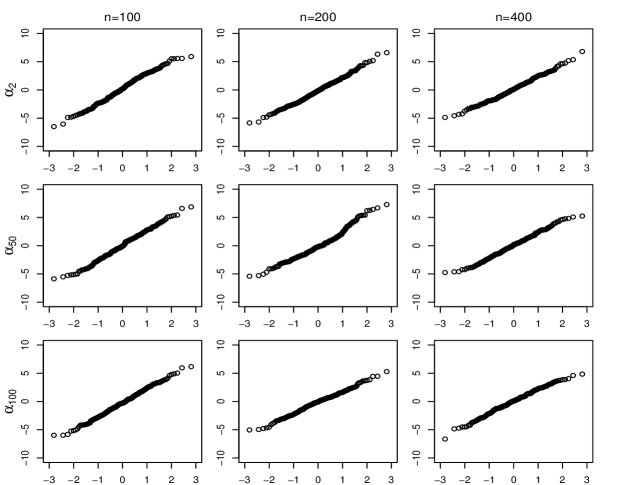
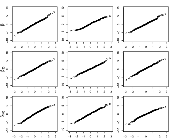
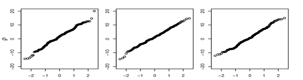
Figure 1: The Q-Q plots of the error (group 1).

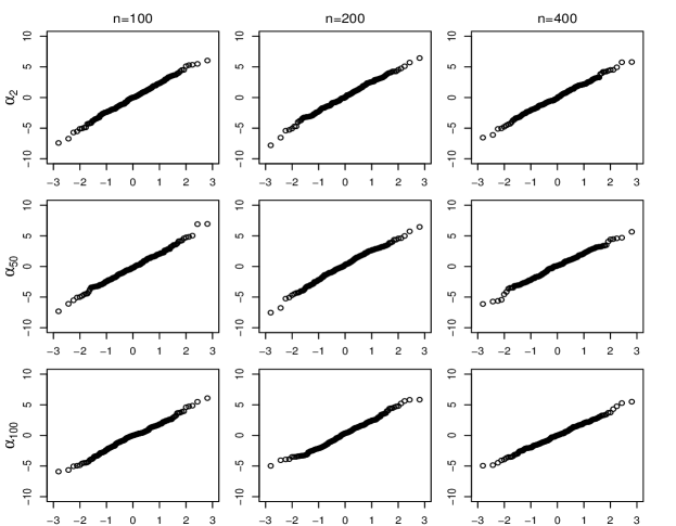
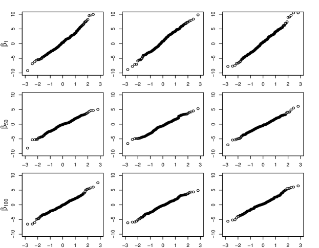
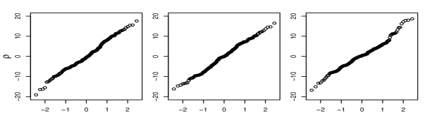
Figure 2: The Q-Q plots of the error (group 2).

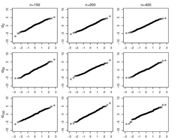
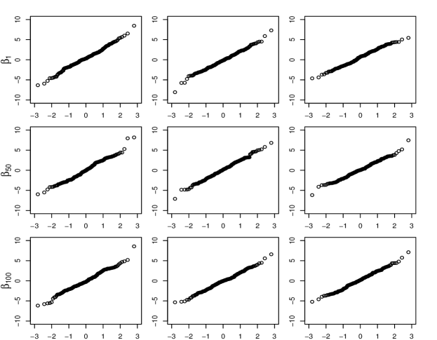
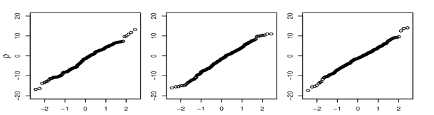
Figure 3: The Q-Q plots of the error (group 3).

3.2 Uniform consistency condition

The purpose of this subsection is to check if uniform consistency holds under much weaker condition than that in corollary 2.7. We conduct one group of experiment, figure 4, on model (3) with $\mu_{n}=10\cdot n^{-\frac{2}{3}}$ being known, $\alpha_{1}=0$; $\alpha_{i}(i\neq 1),\beta_{i}$ being independently uniformly distributed over [-1,1] and $\rho=0.3$. We use the following algorithm to approximate the maximizer of the likelihood:

Algorithm 2 Coordinate descent and gradient descent

$\alpha_{i}^{(0)}=\alpha_{i}^{*};\beta_{i}^{(0)}=\beta_{i}^{*};\rho^{(0)}=\rho^{*}$;$t=0$;

while  $e^{(t)}<0.05$  do

     for  $i=1,2,\cdots,n+1$ do

         if  $i\leq n$ then

              maximize $\ell_{i}$ with respect to $\alpha_{i},\beta_{i}$ by gradient descent algorithm, i.e.,

              iteratively update $\alpha_{i},\beta_{i}$ as in gradient descent algorithm until the following sub-stopping-criterion is

              reached:

              $e_{i,s}=\max\{\ |\frac{\partial\ell_{i}}{\partial\alpha_{i}}(\boldsymbol{\alpha}_{-i}^{(t-1)},\boldsymbol{\beta}_{-i}^{(t-1)},\alpha_{i}^{s},\beta_{i}^{s},\rho^{(t-1)},\mu_{n})|,|\frac{\partial\ell_{i}}{\partial\beta_{i}}(\boldsymbol{\alpha}_{-i}^{(t-1)},\boldsymbol{\beta}_{-i}^{(t-1)},\alpha_{i}^{s},\beta_{i}^{s},\rho^{(t-1)},\mu_{n})|\ \}<10^{-3}$.

              Where $\alpha_{i}^{s},\beta_{i}^{s}$ refers to the updated $\alpha_{i},\beta_{i}$ after the $s^{th}$ iteration and $\alpha_{i}^{0}=\alpha_{i}^{(t-1)},\beta_{i}^{0}=\beta_{i}^{(t-1)}$.

         else $i=n+1$

              update $\rho$ in the same way.

         end if

     end for

     Let $\boldsymbol{\alpha}^{(t)},\boldsymbol{\beta}^{(t)},\rho^{(t)}$ be the parameter vector after the $t^{th}$ round iteration.

     Let $e^{(t)}=\sup\limits_{i\leq n}\big{\{}\ |\frac{\partial\ell_{i}}{\partial\alpha_{i}}(\boldsymbol{\alpha}^{(t)},\boldsymbol{\beta}^{(t)},\rho^{(t)},\mu_{n})|,|\frac{\partial\ell_{i}}{\partial\beta_{i}}(\boldsymbol{\alpha}^{(t)},\boldsymbol{\beta}^{(t)},\rho^{(t)},\mu_{n})|,|\frac{\partial\ell}{\partial\rho}(\boldsymbol{\alpha}^{(t)},\boldsymbol{\beta}^{(t)},\rho^{(t)},\mu_{n})|\ \big{\}}$.

     t = t+1;

end while

We generate networks of size $n=400,1400$ and $5000$ by model (3). In each setting 30 replications are used. The parameters and the initial value of parameters in the optimization algorithm are fixed through out all replications. We use mean square error bound, namely $\frac{1}{n}\sum\limits_{i\leq n}\big{(}\ |\hat{\alpha}_{i}-\alpha_{i}^{*}|^{2}+|\hat{\beta}_{i}-\beta_{i}^{*}|^{2}\big{)}$, as the weak consistency measure. We use uniform error bound, namely $\sup\limits_{i\leq n}\big{\{}\ |\hat{\alpha}_{i}-\alpha_{i}^{*}|^{2}+|\hat{\beta}_{i}-\beta_{i}^{*}|^{2}\ \big{\}}$, as the uniform consistency measure. The results show that, both mean square error bound (subfigure 4(a)) and the uniform error bound (subfigure 4(b)) decreases as $n$ increases.

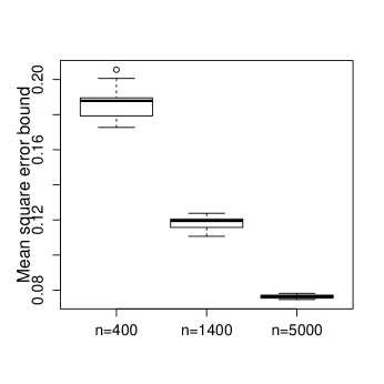
(a) Mean square error bound

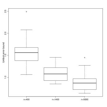
(b) Uniform error bound

Figure 4: Consistency under weaker condition

3.3 Overfitting

In this subsection, our results show that the MLE can be overfitting. Because the uniform error bound can be reduced when the stopping criterion is relaxed. Meanwhile, the mean square error bound is not reduced. We conduct one group of experiment, figure 4, on the exponential network model (3) with $\mu_{n}=10\cdot n^{-\frac{2}{3}}$ being known, $\alpha_{1}=0$; $\alpha_{i}(i\neq 1),\beta_{i}$ being independently uniformly distributed over [-1,1] and $\rho=0.3$. We use the following algorithm to approximate the maximizer of the likelihood. Let $\varepsilon_{i},\varepsilon^{\prime}_{i}$ be independent and uniformly distributed over [-0.5,0.5].

Algorithm 3 Coordinate descent and gradient descent

$\alpha_{i}^{(0)}=\alpha_{i}^{*}+\varepsilon_{i};\beta_{i}^{(0)}=\beta_{i}^{*}+\varepsilon^{\prime}_{i};$ $\rho^{(0)}=\rho^{*}$;$t=0$;

while  $e^{(t)}<e$  do

     for  $i=1,2,\cdots,n+1$ do

         if  $i\leq n$ then

              maximize $\ell_{i}$ with respect to $\alpha_{i},\beta_{i}$ by gradient descent algorithm, i.e.,

              iteratively update $\alpha_{i},\beta_{i}$ as in gradient descent algorithm until the following sub-stopping-criterion is

              reached:

              $e_{i,s}=\max\{\ |\frac{\partial\ell_{i}}{\partial\alpha_{i}}(\boldsymbol{\alpha}_{-i}^{(t-1)},\boldsymbol{\beta}_{-i}^{(t-1)},\alpha_{i}^{s},\beta_{i}^{s},\rho^{(t-1)},\mu_{n})|,|\frac{\partial\ell_{i}}{\partial\beta_{i}}(\boldsymbol{\alpha}_{-i}^{(t-1)},\boldsymbol{\beta}_{-i}^{(t-1)},\alpha_{i}^{s},\beta_{i}^{s},\rho^{(t-1)},\mu_{n})|\ \}<10^{-3}$.

              Where $\alpha_{i}^{s},\beta_{i}^{s}$ refers to the updated $\alpha_{i},\beta_{i}$ after the $s^{th}$ iteration and $\alpha_{i}^{0}=\alpha_{i}^{(t-1)},\beta_{i}^{0}=\beta_{i}^{(t-1)}$.

         else $i=n+1$

              update $\rho$ in the same way.

         end if

     end for

     Let $\boldsymbol{\alpha}^{(t)},\boldsymbol{\beta}^{(t)},\rho^{(t)}$ be the parameter vector after the $t^{th}$ round iteration.

     Let $e^{(t)}=\sup\limits_{i\leq n}\big{\{}\ |\frac{\partial\ell_{i}}{\partial\alpha_{i}}(\boldsymbol{\alpha}^{(t)},\boldsymbol{\beta}^{(t)},\rho^{(t)},\mu_{n})|,|\frac{\partial\ell_{i}}{\partial\beta_{i}}(\boldsymbol{\alpha}^{(t)},\boldsymbol{\beta}^{(t)},\rho^{(t)},\mu_{n})|,|\frac{\partial\ell}{\partial\rho}(\boldsymbol{\alpha}^{(t)},\boldsymbol{\beta}^{(t)},\rho^{(t)},\mu_{n})|\ \big{\}}$.

     t = t+1;

end while

We refer to the constant $e$ in the above algorithm as the stopping criterion. We generate networks of size $n=1000,2000$ by model (3) and test the algorithm for $e=0.08,0.02$. In each setting 30 replications are used. The parameters and the initial value of parameters in the optimization algorithm are fixed through out all replications. Figure 5 shows how mean square error bound (subfigure 5(a)) and uniform error bound (subfigure 5(b)) vary with stopping criterion $e$. Both error bounds are not explicitly reduced when $e$ decreases.

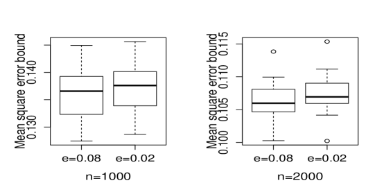
(a) Mean square error bound

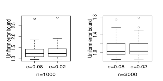
(b) Uniform error bound

Figure 5: Overfitting

4 Conclusion

Our results confirm that the condition ensuring weak consistency in continuous parameter case is almost the same as that in discrete parameter case. But the uniform consistency condition we obtained is stronger than that in the discrete parameter case. It is not clear if the uniform consistency condition in the continuous parameter case is necessarily stronger than that in the discrete parameter case. Our experiments in section 3.1 show that the MLE in the exponential network model with interaction effect might be asymptotically normal when $\mu_{n}=1$. This is stronger than the consistency results we proved. The experiments in section 3.2 also show that it is possible that uniform consistency condition holds under much weaker condition than that in corollary 2.7. However, the experiment in section 3.3 shows that relaxing the stopping criterion somehow reduces uniform error bound. This indicates that in continuous parameter case, MLE may indeed overfit. We take this as an indirect evidence confirming that the uniform consistency condition in continuous parameter case is necessarily stronger (but may not be necessarily as strong as that in corollary 2.7). We also show that by applying the MLE on the discretized parameter space, the uniform consistency condition is almost the same as that in the discrete parameter case.

5 Proof

5.1 Proof of theorem 2.4

The proof of theorem 2.4 concern bounding the fluctuation of log likelihood on the whole parameter space. We firstly establish an auxiliary lemma on the fluctuation of the sum of independent discrete random variable.

Lemma 5.1.

Suppose $Z_{i},i\leq m$ are $m$ independent random variables with $|Z_{i}|\leq C_{m}$. There is a univeral constant $c_{0}$ such that for any $u$, if $\dfrac{|u|}{\sum\limits_{i\leq m}\operatorname{E}[Z_{i}^{2}]}<\frac{c_{0}}{C_{m}}$, let $Z=\sum\limits_{i\leq m}Z_{i}$, then we have,

$$\mathbb{P}\bigg{(}\big{|}Z-\operatorname{E}[Z]\big{|}\geq u\bigg{)}\leq\exp\bigg{\{}-\frac{u^{2}}{2\sum\limits_{i\leq m}\operatorname{E}[Z_{i}^{2}]}+\frac{u^{3}\sum\limits_{i\leq m}\operatorname{E}[|Z_{i}|^{3}]}{\big{(}\sum\limits_{i\leq m}\operatorname{E}[Z_{i}^{2}]\big{)}^{3}}\bigg{\}}.$$ (9)

Proof.

The proof concern Chernoff inequality:

$$\mathbb{P}\bigg{(}Z-\operatorname{E}[Z]\leq-u\bigg{)}\leq\inf\limits_{t<0}\exp\big{\{}\log(\operatorname{E}[e^{tZ}])-\operatorname{E}[tZ]+tu\big{\}}.$$ (10)

Note that $\log(\operatorname{E}[e^{tZ}])=\sum\limits_{i\leq m}\log\operatorname{E}[e^{tZ_{i}}]$. Therefore if $|t|<\frac{c_{0}}{C_{m}}$, by Taylor expansion

$$\log\operatorname{E}[e^{tZ_{i}}]\leq t\operatorname{E}[Z_{i}]+\frac{1}{2}t^{2}\operatorname{E}[Z_{i}^{2}]+|t|^{3}\operatorname{E}[|Z_{i}|^{3}].$$ (11)

Set $t=-\dfrac{u}{\sum\limits_{i\leq m}\operatorname{E}[Z_{i}^{2}]}$, so $|t|<\frac{c_{0}}{C_{m}}$. Therefore substitute (11) into (10) we have,

$$\mathbb{P}\bigg{(}Z-\operatorname{E}[Z]\leq-u\bigg{)}\leq\exp\big{\{}-\dfrac{u^{2}}{2\sum\limits_{i\leq m}\operatorname{E}[Z_{i}^{2}]}+\dfrac{u^{3}\sum\limits_{i\leq m}\operatorname{E}[|Z_{i}|^{3}]}{\big{(}\sum\limits_{i\leq m}\operatorname{E}[Z_{i}^{2}]\big{)}^{3}}\big{\}}.$$ (12)

It is similar to prove the other direction.

∎

Lemma 5.2.

$$\sup\limits_{\boldsymbol{\eta}\in\mathcal{B}_{1}\times\cdots\times\mathcal{B}_{n},\boldsymbol{\rho}\in\mathcal{B},\mu_{n}\in[\frac{1}{n},1]}\bigg{|}\ell(\mathbf{Y};\boldsymbol{\eta},\boldsymbol{\rho},\mu_{n})-\operatorname{E}\big{[}\ell(\mathbf{Y};\boldsymbol{\eta},\boldsymbol{\rho},\mu_{n})\ \big{]}\bigg{|}=O_{p}(n^{\frac{3}{2}}\sqrt{\mu_{n}^{*}}(\log n)^{2}).$$ (13)

Proof.

Since $\mathcal{B}$ is compact by assumption 2.3 item (1), we cover $\mathcal{B}_{1}\times\cdots\times\mathcal{B}_{n}$ with $n^{2n}$ many points, cover $\mathcal{B}$ with $n^{2}$ many points, cover $[\frac{1}{n},1]$ with $n^{3}$ many points such that for every $\boldsymbol{\eta}\in\mathcal{B}_{1}\times\cdots\times\mathcal{B}_{n},\boldsymbol{\rho}\in\mathcal{B},\mu_{n}\in[\frac{1}{n},1]$ there exists a covering point such that the log likelihood on the covering point is close to that on $\boldsymbol{\eta},\boldsymbol{\rho}\in\mathcal{B},\mu_{n}$. So it suffices to show that

$$\sup\limits_{(\boldsymbol{\eta},\boldsymbol{\rho},\mu_{n})\in B_{n}}\bigg{|}\ell(\mathbf{Y};\boldsymbol{\eta},\boldsymbol{\rho},\mu_{n})-\operatorname{E}\big{[}\ell(\mathbf{Y};\boldsymbol{\eta},\boldsymbol{\rho},\mu_{n})\ \big{]}\bigg{|}=O_{p}(n^{\frac{3}{2}}\sqrt{\mu_{n}^{*}}(\log n)^{2}),$$ (14)

where $B_{n}$ is the covering set. By assumption 2.3 item (2) on $f$ and the fact $\mu_{n}^{*}\geq\frac{1}{n}$, we have:

$$|\ell_{ij}(Y_{ij};\boldsymbol{\eta}_{i},\boldsymbol{\eta}_{j},\boldsymbol{\rho},\mu_{n})|\leq 2\log n,$$ (15)

$$\sum\limits_{i<j\leq n}\operatorname{E}\big{[}|\ell_{ij}(Y_{ij};\boldsymbol{\eta}_{i},\boldsymbol{\eta}_{j},\boldsymbol{\rho},\mu_{n})|^{3}\big{]}=O(\mu_{n}^{*}n^{2}(\log n)^{3}),$$

$$\sum\limits_{i<j\leq n}\operatorname{E}\big{[}|\ell_{ij}(Y_{ij};\boldsymbol{\eta}_{i},\boldsymbol{\eta}_{j},\boldsymbol{\rho},\mu_{n})|^{2}\big{]}=\Theta(\mu_{n}^{*}n^{2}(\log n)^{2}).$$

Set $u=n^{\frac{3}{2}}\sqrt{\mu_{n}^{*}}(\log n)^{2}$. Clearly, by condition on $\mu_{n}^{*}$ in theorem 2.4

$$\dfrac{u}{\sum\limits_{i<j\leq n}\operatorname{E}[|\ell_{ij}(Y_{ij};\boldsymbol{\eta}_{i},\boldsymbol{\eta}_{j},\boldsymbol{\rho},\mu_{n})|^{2}]}=O(\frac{1}{\sqrt{\mu_{n}^{*}n}})=o(\frac{1}{\log n}).$$

So the condition of lemma 5.1 on $u$ is satisfied. Furthermore,

$$\dfrac{u^{3}\sum\limits_{i<j\leq n}\operatorname{E}[|\ell_{ij}(Y_{ij};\boldsymbol{\eta}_{i},\boldsymbol{\eta}_{j},\boldsymbol{\rho},\mu_{n})|^{3}]}{\big{(}\sum\limits_{i<j\leq n}\operatorname{E}[|\ell_{ij}(Y_{ij};\boldsymbol{\eta}_{i},\boldsymbol{\eta}_{j},\boldsymbol{\rho},\mu_{n})|^{2}]\big{)}^{3}}=O(n^{\frac{1}{2}}(\mu_{n}^{*})^{-\frac{1}{2}}(\log n)^{3}).$$ (16)

Therefore by Borel Cantali’s lemma and lemma 5.1,

$$\mathbb{P}\bigg{(}\sup\limits_{(\boldsymbol{\eta},\boldsymbol{\rho},\mu_{n})\in B_{n}}\bigg{|}\ell(\mathbf{Y};\boldsymbol{\eta},\boldsymbol{\rho},\mu_{n})-\operatorname{E}\big{[}\ell(\mathbf{Y};\boldsymbol{\eta},\boldsymbol{\rho},\mu_{n})\ \big{]}\bigg{|}\geq u\bigg{)}$$ (17)

$$\leq \exp\bigg{\{}O(n\log n)-\dfrac{u^{2}}{\sum\limits_{i<j\leq n}\operatorname{E}[|\ell_{ij}(Y_{ij};\boldsymbol{\eta}_{i},\boldsymbol{\eta}_{j},\boldsymbol{\rho},\mu_{n})|^{2}]}+O(n^{\frac{1}{2}}(\mu_{n}^{*})^{-\frac{1}{2}}(\log n)^{3})\bigg{\}}$$

$$\leq \exp\big{\{}O(n\log n)-\Omega(n(\log n)^{2})+O(n^{\frac{1}{2}}(\mu_{n}^{*})^{-\frac{1}{2}}(\log n)^{3})\big{\}}$$

$$\text{ by condition on }\mu_{n}^{*}\text{ in theorem \ref{asymth5}},(\log n)^{2}=o(\mu^{*}_{n}n)$$

$$\rightarrow 0$$

∎

Now it is direct to prove theorem 2.4. Let $\overline{\mu}_{n}=\frac{1}{n(n-1)}\sum\limits_{i\neq j\leq n}I(Y_{ij}\neq\mathbf{0})$ if $\mu_{n}$ represent average degree; and for notation consistency, set $\overline{\mu}_{n}=\mu_{n}^{*}$ when $\mu_{n}$ is known. Calculating the variance of $\overline{\mu}_{n}$, we have $|\overline{\mu}_{n}-\mu_{n}^{*}|=O_{p}(\frac{\sqrt{\mu_{n}^{*}}}{n})$. So by assumption 2.3 item (2),

$$\big{|}\ell(\mathbf{Y};\boldsymbol{\eta},\boldsymbol{\rho},\overline{\mu}_{n})-\ell(\mathbf{Y};\boldsymbol{\eta},\boldsymbol{\rho},\mu_{n}^{*})\big{|}=O_{p}(n\sqrt{\mu_{n}^{*}})$$

uniformly in $\boldsymbol{\eta},\boldsymbol{\rho}$. Let $\mathbf{X}$ be an independent copy of $\mathbf{Y}$. By lemma 5.2,

$$\ell(\mathbf{Y};\boldsymbol{\eta}^{*},\boldsymbol{\rho}^{*},\mu_{n}^{*})-\operatorname{E}\big{[}\ell(\mathbf{Y};\boldsymbol{\eta}^{*},\boldsymbol{\rho}^{*},\mu_{n}^{*})\big{]},$$ (18)

$$\ell(\mathbf{Y};\boldsymbol{\hat{\eta}},\hat{\boldsymbol{\rho}},\mu_{n}^{*})-\operatorname{E}_{\mathbf{X}}\big{[}\ell(\mathbf{X};\boldsymbol{\hat{\eta}},\hat{\boldsymbol{\rho}},\mu_{n}^{*})\big{]}$$

$$= O_{p}(n^{\frac{3}{2}}\sqrt{\mu_{n}^{*}}(\log n)^{2}).$$

Also note that,

$$\big{|}\ell(\mathbf{Y};\boldsymbol{\hat{\eta}},\hat{\boldsymbol{\rho}},\overline{\mu}_{n})-\ell(\mathbf{Y};\boldsymbol{\hat{\eta}},\hat{\boldsymbol{\rho}},\mu_{n}^{*})\big{|}=O_{p}(n\sqrt{\mu_{n}^{*}}),$$ (19)

$$\ell(\mathbf{Y};\boldsymbol{\hat{\eta}},\hat{\boldsymbol{\rho}},\overline{\mu}_{n})\geq\ell(\mathbf{Y};\boldsymbol{\eta}^{*},\boldsymbol{\rho}^{*},\overline{\mu}_{n}),\text{ since }\boldsymbol{\hat{\eta}}\text{ is MLE.}$$

$$\operatorname{E}_{\mathbf{X}}\big{[}\ell(\mathbf{X};\boldsymbol{\hat{\eta}},\hat{\boldsymbol{\rho}},\mu_{n}^{*})\big{]}\leq\operatorname{E}\big{[}\ell(\mathbf{Y};\boldsymbol{\eta}^{*},\boldsymbol{\rho}^{*},\mu_{n}^{*})\big{]}.$$

Thus combine (18)(19),

$$\bigg{|}\operatorname{E}_{\mathbf{X}}\big{[}\ell(\mathbf{X};\boldsymbol{\hat{\eta}},\hat{\boldsymbol{\rho}},\mu_{n}^{*})\big{]}-\operatorname{E}\big{[}\ell(\mathbf{Y};\boldsymbol{\eta}^{*},\boldsymbol{\rho}^{*},\mu_{n}^{*})\big{]}\bigg{|}=O_{p}(n^{\frac{3}{2}}\sqrt{\mu_{n}^{*}}(\log n)^{2}+n\sqrt{\mu_{n}^{*}}).$$ (20)

Meanwhile, (20) together with the assumption $c\leq f\leq C$ imply that

$$\mu_{n}^{*}\sum\limits_{i<j\leq n}||f(\cdot;\hat{\boldsymbol{\eta}}_{i},\hat{\boldsymbol{\eta}}_{j},\hat{\boldsymbol{\rho}})-f(\cdot;\boldsymbol{\eta}_{i}^{*},\boldsymbol{\eta}_{j}^{*},\boldsymbol{\rho}^{*})||_{2}^{2}=O_{p}(n^{\frac{3}{2}}\sqrt{\mu_{n}^{*}}(\log n)^{2}).$$ (21)

So the proof is accomplished.

5.2 Proof of corollary 2.5

The conclusion of theorem 2.4 together with assumption 2.3 item (3) imply that for some true parameter $\boldsymbol{\eta}^{*}$,

$$\mu_{n}^{*}n\sum\limits_{i\leq n}||\hat{\boldsymbol{\eta}}_{i}-\boldsymbol{\eta}_{i}^{*}||_{2}^{2}+\mu_{n}^{*}n^{2}||\hat{\boldsymbol{\rho}}-\boldsymbol{\rho}^{*}||_{2}^{2}=O_{p}(n^{\frac{3}{2}}\sqrt{\mu_{n}^{*}}(\log n)^{2}).$$

Or equivalently,

$$\sum\limits_{i\leq n}||\hat{\boldsymbol{\eta}}_{i}-\boldsymbol{\eta}_{i}^{*}||_{2}^{2}=n^{\frac{1}{2}}(\mu_{n}^{*})^{-\frac{1}{2}}(\log n)^{2},$$

$$||\hat{\boldsymbol{\rho}}-\boldsymbol{\rho}^{*}||_{2}^{2}=n^{-\frac{1}{2}}(\mu_{n}^{*})^{-\frac{1}{2}}(\log n)^{2}.$$

5.3 Proof of theorem 2.6

The key observation is the following:

$$\sup\limits_{i\leq n,\boldsymbol{\eta}_{i}\in\mathcal{B}_{i}}\ell_{i}(\mathbf{Y};\boldsymbol{\eta}_{i},\boldsymbol{\boldsymbol{\eta}}_{-i}^{*},\boldsymbol{\rho}^{*},\mu_{n}^{*})-\operatorname{E}\big{[}\ell_{i}(\mathbf{Y};\boldsymbol{\eta}_{i},\boldsymbol{\eta}_{-i}^{*},\boldsymbol{\rho}^{*},\mu_{n}^{*})\big{]}=O_{p}(n^{\frac{1}{2}}(\mu_{n}^{*})^{\frac{1}{2}}(\log n)^{\frac{3}{2}}).$$ (22)

(22) follows by standard covering method, concentration inequality (lemma 5.1) plus Borel Cantelli’s lemma. Here the space to be covered is $\cup_{i\leq n}\mathcal{B}_{i}$, which is substantially smaller than that in the proof of theorem 2.4 (namely $\mathcal{B}_{1}\times\cdots\times\mathcal{B}_{n}$).

Another fact implied by assumption 2.3 item (4) is

$$\sup\limits_{i}\bigg{|}\ell_{i}(\mathbf{Y};\boldsymbol{\eta}_{i},\boldsymbol{\eta}_{-i}^{*},\boldsymbol{\rho}^{*},\mu_{n}^{*})-\ell_{i}(\mathbf{Y};\boldsymbol{\eta}_{i},\boldsymbol{\eta}_{-i},\boldsymbol{\rho},\mu_{n})\bigg{|}$$ (23)

$$= O(||\boldsymbol{\boldsymbol{\eta}}-\boldsymbol{\eta}^{*}||_{1,\mathbf{Y}_{i}})+O_{p}(\mu_{n}^{*}\log n||\boldsymbol{\boldsymbol{\eta}}-\boldsymbol{\eta}^{*}||_{1}+\mu_{n}^{*}n\log n||\boldsymbol{\rho}-\boldsymbol{\rho}^{*}||_{1}+n\log n|\overline{\mu}_{n}-\mu_{n}^{*}|).$$

In notation $||\boldsymbol{\eta}-\boldsymbol{\eta}^{*}||_{1,\mathbf{Y}_{i}}$, $\mathbf{Y}_{i}$ is regarded as a $0-1$ sequence $(I(Y_{i1}\neq\mathbf{0}),I(Y_{i2}\neq\mathbf{0}),\cdots,I(Y_{in}\neq\mathbf{0}))$. To see this note that: for $y\neq\mathbf{0}$, by assumption 2.3 item (4)

$$\big{|}\ell_{ij}(y;\boldsymbol{\eta}_{i},\boldsymbol{\eta}_{j}^{*},\boldsymbol{\rho}^{*},\mu_{n}^{*})-\ell_{ij}(y;\boldsymbol{\eta}_{i},\boldsymbol{\eta}_{j},\boldsymbol{\rho},\mu_{n})\big{|}$$ (24)

$$= O(||\boldsymbol{\eta}_{j}-\boldsymbol{\eta}_{j}^{*}||_{1}+||\boldsymbol{\eta}_{i}-\boldsymbol{\eta}_{i}^{*}||_{1}+||\boldsymbol{\rho}-\boldsymbol{\rho}^{*}||_{1}+\frac{1}{\mu_{n}^{*}}|\overline{\mu}_{n}-\mu_{n}^{*}|)$$

, and

$$\big{|} \ell_{ij}(\mathbf{0};\boldsymbol{\eta}_{i},\boldsymbol{\eta}_{j}^{*},\boldsymbol{\rho}^{*},\mu_{n}^{*})-\ell_{ij}(\mathbf{0};\boldsymbol{\eta}_{i},\boldsymbol{\eta}_{j},\boldsymbol{\rho},\mu_{n})\big{|}$$ (25)

$$= O(\mu_{n}^{*}||\boldsymbol{\eta}_{j}-\boldsymbol{\eta}_{j}^{*}||_{1}+\mu_{n}^{*}||\boldsymbol{\eta}_{i}-\boldsymbol{\eta}_{i}^{*}||_{1}+\mu_{n}^{*}||\boldsymbol{\rho}-\boldsymbol{\rho}^{*}||_{1}+|\overline{\mu}_{n}-\mu_{n}^{*}|).$$

Equation (24) explains the term $||\boldsymbol{\boldsymbol{\eta}}-\boldsymbol{\eta}^{*}||_{1,\mathbf{Y}_{i}}$ in (23). The other terms in (23) are explained by (25)(24) and the following fact:

$$\sup\limits_{i}\sum\limits_{j\leq n}I(Y_{ij}=\mathbf{0})=O_{p}(\mu_{n}^{*}n\log n).$$ (26)

(26) follow by applying lemma 5.1 plus Borel-Cantelli’s lemma by standard procedure.

Lemma 5.3.

For every $\varepsilon>0$ there exists $C_{\varepsilon}$ such that with probability at least $1-\varepsilon$ the following holds:

$$\sup\limits_{i}\ n\mu_{n}^{*}\cdot||\hat{\boldsymbol{\eta}}_{i}-\boldsymbol{\eta}^{*}_{i}||_{2}^{2}\ \leq\ C_{\varepsilon}\big{(}\ ||\boldsymbol{\hat{\eta}}-\boldsymbol{\eta}^{*}||_{1,\mathbf{Y}_{i}}+\mu_{n}^{*}\log n\sqrt{n\Delta_{\eta}}+\mu_{n}^{*}n\log n\sqrt{\Delta_{\rho}}+n^{\frac{1}{2}}(\mu_{n}^{*})^{\frac{1}{2}}(\log n)^{\frac{3}{2}}\ \big{)}.$$ (27)

Proof.

Using Cauchy-Schwartz inequality we have $\sum\limits_{i\leq n}||\hat{\boldsymbol{\eta}}_{i}-\boldsymbol{\eta}^{*}_{i}||_{1}=O(\sqrt{n\Delta_{\eta}})$. Also note that $n|\overline{\mu}_{n}-\mu_{n}^{*}|=O_{p}(1)$. Therefore using (23), we have uniformly in $i,\boldsymbol{\eta}_{i}$:

$$\big{|}\ell_{i}(\mathbf{Y}_{i};\boldsymbol{\eta}_{i},\boldsymbol{\eta}_{-i}^{*},\boldsymbol{\rho}^{*},\mu_{n}^{*})-\ell_{i}(\mathbf{Y}_{i};\boldsymbol{\eta}_{i},\boldsymbol{\hat{\eta}}_{-i},\hat{\boldsymbol{\rho}},\overline{\mu}_{n})\big{|}$$ (28)

$$= O(||\boldsymbol{\hat{\eta}}-\boldsymbol{\eta}^{*}||_{1,\mathbf{Y}_{i}})+O_{p}(\mu_{n}^{*}\log n\sqrt{n\Delta_{\eta}}+\mu_{n}^{*}n\log n\sqrt{\Delta_{\rho}}+\log n\sqrt{\mu_{n}^{*}}).$$

Note that for all $i\leq n$,

$$\ell_{i}(\mathbf{Y}_{i};\hat{\boldsymbol{\eta}}_{i},\boldsymbol{\hat{\eta}}_{-i},\hat{\boldsymbol{\rho}},\overline{\mu}_{n})\geq\ell_{i}(\mathbf{Y}_{i};\boldsymbol{\eta}_{i}^{*},\boldsymbol{\hat{\eta}}_{-i},\hat{\boldsymbol{\rho}},\overline{\mu}_{n}),$$ (29)

since $\hat{\boldsymbol{\eta}}$ is MLE. While for all $i\leq n$

$$\operatorname{E}_{\mathbf{X}_{i}}\big{[}\ell_{i}(\mathbf{X}_{i};\hat{\boldsymbol{\eta}}_{i},\boldsymbol{\hat{\eta}}_{-i},\hat{\boldsymbol{\rho}},\overline{\mu}_{n})\big{]}\leq\operatorname{E}_{\mathbf{Y}_{i}}\big{[}\ell_{i}(\mathbf{Y}_{i};\boldsymbol{\eta}_{i}^{*},\boldsymbol{\eta}_{-i}^{*},\boldsymbol{\rho}^{*},\mu_{n}^{*})\big{]}.$$ (30)

By assumption 2.3 item (4) and using Cauchy-Schwarz inequality, we have, uniformly in $i$:

$$\bigg{|}\ \operatorname{E}_{\mathbf{X}_{i}}\big{[}\ell_{i}(\mathbf{X}_{i};\boldsymbol{\eta}_{i}^{*},\boldsymbol{\hat{\eta}}_{-i},\hat{\boldsymbol{\rho}},\overline{\mu}_{n})\big{]}-\operatorname{E}_{\mathbf{X}_{i}}\big{[}\ell_{i}(\mathbf{X}_{i};\boldsymbol{\eta}_{i}^{*},\boldsymbol{\eta}_{-i}^{*},\boldsymbol{\rho}^{*},\mu_{n}^{*})\big{]}\ \bigg{|}=O_{p}(\mu_{n}^{*}\log n\sqrt{n\Delta_{\eta}}+\mu_{n}^{*}n\log n\sqrt{\Delta_{\rho}}+\log n\sqrt{\mu_{n}^{*}}).$$ (31)

By (30)(31), uniformly in $i$:

$$\operatorname{E}_{\mathbf{X}_{i}}\big{[}\ell_{i}(\mathbf{X}_{i};\hat{\boldsymbol{\eta}}_{i},\boldsymbol{\hat{\eta}}_{-i},\hat{\boldsymbol{\rho}},\overline{\mu}_{n})\big{]}\leq\operatorname{E}_{\mathbf{X}_{i}}\big{[}\ell_{i}(\mathbf{X}_{i};\boldsymbol{\eta}_{i}^{*},\boldsymbol{\hat{\eta}}_{-i},\hat{\boldsymbol{\rho}},\overline{\mu}_{n})\big{]}+O_{p}(\mu_{n}^{*}\log n\sqrt{n\Delta_{\eta}}+\mu_{n}^{*}n\log n\sqrt{\Delta_{\rho}}+\log n\sqrt{\mu_{n}^{*}}).$$ (32)

Combine (28),(22) we have, uniformly in $i$,

$$\bigg{|}\ell_{i}(\mathbf{Y}_{i};\hat{\boldsymbol{\eta}}_{i},\boldsymbol{\hat{\eta}}_{-i},\hat{\boldsymbol{\rho}},\overline{\mu}_{n})-\operatorname{E}_{\mathbf{X}_{i}}\big{[}\ell_{i}(\mathbf{X}_{i};\hat{\boldsymbol{\eta}}_{i},\boldsymbol{\hat{\eta}}_{-i},\hat{\boldsymbol{\rho}},\overline{\mu}_{n})\big{]}\ \bigg{|},$$ (33)

$$\bigg{|}\ \ell_{i}(\mathbf{Y}_{i};\boldsymbol{\eta}_{i}^{*},\boldsymbol{\hat{\eta}}_{-i},\hat{\boldsymbol{\rho}},\overline{\mu}_{n})-\operatorname{E}_{\mathbf{X}_{i}}\big{[}\ell_{i}(\mathbf{X}_{i};\boldsymbol{\eta}_{i}^{*},\boldsymbol{\hat{\eta}}_{-i},\hat{\boldsymbol{\rho}},\overline{\mu}_{n})\big{]}\ \bigg{|}$$

$$= O(||\boldsymbol{\hat{\boldsymbol{\eta}}}-\boldsymbol{\eta}^{*}||_{1,\mathbf{Y}_{i}})+O_{p}(\mu_{n}^{*}\log n\sqrt{n\Delta_{\eta}}+\mu_{n}^{*}n\log n\sqrt{\Delta_{\rho}})+O_{p}(n^{\frac{1}{2}}(\mu_{n}^{*})^{\frac{1}{2}}(\log n)^{\frac{3}{2}}).$$

Thus combine (29),(32) with (33) we have, uniformly in $i$,

$$\bigg{|}\operatorname{E}_{\mathbf{X}_{i}}\big{[}\ell_{i}(\mathbf{X}_{i};\hat{\boldsymbol{\eta}}_{i},\boldsymbol{\hat{\eta}}_{-i},\hat{\boldsymbol{\rho}},\overline{\mu}_{n})\big{]}\ -\operatorname{E}_{\mathbf{X}_{i}}\big{[}\ell_{i}(\mathbf{X}_{i};\boldsymbol{\eta}_{i}^{*},\boldsymbol{\hat{\eta}}_{-i},\hat{\boldsymbol{\rho}},\overline{\mu}_{n})\big{]}\bigg{|}$$ (34)

$$= O(||\boldsymbol{\hat{\eta}}-\boldsymbol{\eta}^{*}||_{1,\mathbf{Y}_{i}})+O_{p}(\mu_{n}^{*}\log n\sqrt{n\Delta_{\eta}})+\mu_{n}^{*}n\log n\sqrt{\Delta_{\rho}})+O_{p}(n^{\frac{1}{2}}(\mu_{n}^{*})^{\frac{1}{2}}(\log n)^{\frac{3}{2}}).$$

Using (28) again, (34) becomes: uniformly in $i$,

$$\bigg{|}\operatorname{E}_{\mathbf{X}_{i}}\big{[}\ell_{i}(\mathbf{X}_{i};\hat{\boldsymbol{\eta}}_{i},\boldsymbol{\eta}_{-i}^{*},\boldsymbol{\rho}^{*},\mu_{n}^{*})\big{]}\ -\operatorname{E}_{\mathbf{Y}_{i}}\big{[}\ell_{i}(\mathbf{Y}_{i};\boldsymbol{\eta}_{i}^{*},\boldsymbol{\eta}_{-i}^{*},\boldsymbol{\rho}^{*},\mu_{n}^{*})\big{]}\bigg{|}$$ (35)

$$= O(||\boldsymbol{\hat{\eta}}-\boldsymbol{\eta}^{*}||_{1,\mathbf{Y}_{i}})+O_{p}(\mu_{n}^{*}\log n\sqrt{n\Delta_{\eta}})+\mu_{n}^{*}n\log n\sqrt{\Delta_{\rho}})+O_{p}(n^{\frac{1}{2}}(\mu_{n}^{*})^{\frac{1}{2}}(\log n)^{\frac{3}{2}}).$$

But by assumption 2.3 item (5),

$$\bigg{|}\operatorname{E}_{\mathbf{X}_{i}}\big{[}\ell_{i}(\mathbf{X}_{i};\hat{\boldsymbol{\eta}}_{i},\boldsymbol{\eta}_{-i}^{*},\boldsymbol{\rho}^{*},\mu_{n}^{*})\big{]}\ -\operatorname{E}_{\mathbf{Y}_{i}}\big{[}\ell_{i}(\mathbf{Y}_{i};\boldsymbol{\eta}_{i}^{*},\boldsymbol{\eta}_{-i}^{*},\boldsymbol{\rho}^{*},\mu_{n}^{*})\big{]}\bigg{|}=\Omega(n\mu_{n}^{*}\cdot||\boldsymbol{\hat{\eta}}_{i}-\boldsymbol{\eta}_{i}^{*}||_{2}^{2})$$

uniformly in $i$. Thus conclusion of lemma 5.3 follows. ∎

Using lemma 5.3 with $||\hat{\boldsymbol{\eta}}-\boldsymbol{\eta}||_{1,\mathbf{Y}_{i}}$ replaced by $||\hat{\boldsymbol{\eta}}-\boldsymbol{\eta}||_{1}$ and applying Cauchy-Schwarz inequality, we easily have:

$$\sup\limits_{i}||\hat{\boldsymbol{\eta}_{i}}-\boldsymbol{\eta}_{i}^{*}||_{2}^{2}=O_{p}(n^{-\frac{1}{2}}\Delta_{\eta}^{\frac{1}{2}}(\mu_{n}^{*})^{-1}\log n+\sqrt{\Delta_{\rho}}\log n+n^{-\frac{1}{2}}(\mu_{n}^{*})^{-\frac{1}{2}}(\log n)^{\frac{3}{2}})$$

Thus the conclusion of theorem 2.6 follows.

5.4 Proof of proposition 2.9

Note that by definition of $\delta_{n}^{\prime}$, the discretized parameter space admit some $\boldsymbol{\tilde{\eta}}$ with $||\boldsymbol{\tilde{\eta}}-\boldsymbol{\eta}^{*}||_{2}^{2}\leq n\delta_{n}^{\prime 2}$ for some true parameter $\boldsymbol{\eta}^{*}$. So by assumption 2.3 item (4) for some constant $C_{f}>0$ depending only on $f$,

$$0\geq\operatorname{E}[\ell(\mathbf{Y};\boldsymbol{\tilde{\eta}},\boldsymbol{\rho}^{*},\mu_{n}^{*})]-\operatorname{E}[\ell(\mathbf{Y};\boldsymbol{\eta}^{*},\boldsymbol{\rho}^{*},\mu_{n}^{*})]\geq-C_{f}\mu_{n}^{*}n^{2}\delta_{n}^{\prime 2}.$$ (36)

But

$$\operatorname{E}[\ell(\mathbf{Y};\boldsymbol{\tilde{\eta}},\boldsymbol{\rho}^{*},\mu_{n}^{*})]\leq\operatorname{E}[\ell(\mathbf{Y};\boldsymbol{\tilde{\eta}}^{*},\boldsymbol{\tilde{\rho}}^{*},\mu_{n}^{*})]\leq\operatorname{E}[\ell(\mathbf{Y};\boldsymbol{\eta}^{*},\boldsymbol{\rho}^{*},\mu_{n}^{*})].$$ (37)

Therefore by assumption 2.3 item (2),

$$\sum\limits_{i<j\leq n}||f(\cdot;\boldsymbol{\tilde{\eta}}_{i}^{*},\boldsymbol{\tilde{\eta}}_{j}^{*},\boldsymbol{\tilde{\rho}}^{*},\mu_{n}^{*})-f(\cdot;\boldsymbol{\eta}_{i}^{*},\boldsymbol{\eta}_{j}^{*},\boldsymbol{\rho}^{*},\mu_{n}^{*})||_{2}^{2}\leq C_{4}n^{2}\delta_{n}^{\prime 2},$$

for some constant $C_{4}>0$ and some true parameter $\boldsymbol{\eta}^{*}$. Thus the conclusion (1) follows from assumption 2.3 item (3).

To prove conclusion (2), for all $i\leq n$, let $\boldsymbol{\tilde{\eta}}_{i}^{\prime}$ be the closest point to $\boldsymbol{\eta}_{i}^{*}$ in $\mathcal{\tilde{B}}_{i}$. So by assumption 2.3 item (4) we have, for some constant $C_{5}^{\prime}$

$$\sup\limits_{i\leq n}\bigg{|}\operatorname{E}[\ell_{i}(\mathbf{Y}_{i};\boldsymbol{\tilde{\eta}}_{i}^{\prime},\boldsymbol{\tilde{\eta}}_{-i}^{*},\boldsymbol{\tilde{\rho}}^{*},\mu_{n}^{*})]-\operatorname{E}[\ell_{i}(\mathbf{Y}_{i};\boldsymbol{\eta}_{i}^{*},\boldsymbol{\eta}_{-i}^{*},\boldsymbol{\rho}^{*},\mu_{n}^{*})]\ \bigg{|}\leq C_{5}^{\prime}\mu_{n}^{*}(n\delta_{n}^{\prime 2}+\Delta_{\eta}+n\Delta_{\rho}).$$ (38)

But

$$\operatorname{E}[\ell_{i}(\mathbf{Y}_{i};\boldsymbol{\tilde{\eta}}_{i}^{\prime},\boldsymbol{\tilde{\eta}}_{-i}^{*},\boldsymbol{\tilde{\rho}}^{*},\mu_{n}^{*})]\leq\operatorname{E}[\ell_{i}(\mathbf{Y}_{i};\boldsymbol{\tilde{\eta}}_{i}^{*},\boldsymbol{\tilde{\eta}}_{-i}^{*},\boldsymbol{\tilde{\rho}}^{*},\mu_{n}^{*})]\leq\operatorname{E}[\ell_{i}(\mathbf{Y}_{i};\boldsymbol{\eta}_{i}^{*},\boldsymbol{\eta}_{-i}^{*},\boldsymbol{\rho}^{*},\mu_{n}^{*})].$$ (39)

Combine (38)(39) we have,

$$\sup\limits_{i\leq n}\bigg{|}\operatorname{E}[\ell_{i}(\mathbf{Y}_{i};\boldsymbol{\tilde{\eta}}_{i}^{*},\boldsymbol{\tilde{\eta}}_{-i}^{*},\boldsymbol{\tilde{\rho}}^{*},\mu_{n}^{*})]-\operatorname{E}[\ell_{i}(\mathbf{Y}_{i};\boldsymbol{\eta}_{i}^{*},\boldsymbol{\eta}_{-i}^{*},\boldsymbol{\rho}^{*},\mu_{n}^{*})]\ \bigg{|}\leq C_{5}^{\prime}\mu_{n}^{*}(n\delta_{n}^{\prime 2}+\Delta_{\eta}+n\Delta_{\rho}),$$

which implies

$$\sup\limits_{i\leq n}\bigg{|}\operatorname{E}[\ell_{i}(\mathbf{Y}_{i};\boldsymbol{\tilde{\eta}}_{i}^{*},\boldsymbol{\eta}_{-i}^{*},\boldsymbol{\rho}^{*},\mu_{n}^{*})]-\operatorname{E}[\ell_{i}(\mathbf{Y}_{i};\boldsymbol{\eta}_{i}^{*},\boldsymbol{\eta}_{-i}^{*},\boldsymbol{\rho}^{*},\mu_{n}^{*})]\ \bigg{|}\leq 2C_{5}^{\prime}\mu_{n}^{*}(n\delta_{n}^{\prime 2}+\Delta_{\eta}+n\Delta_{\rho}).$$

By assumption 2.3 item (5), this implies

$$\sup\limits_{i}||\boldsymbol{\tilde{\eta}}_{i}^{*}-\boldsymbol{\eta}_{i}^{*}||_{2}^{2}=O(\delta_{n}^{\prime 2}+\frac{\Delta_{\eta}}{n}+\Delta_{\rho}).$$

5.5 Proof of theorem 2.11

Note that lemma 5.4 holds with true parameter replaced by pseudo true parameter. i.e., for all $\varepsilon>0$ there exists $C_{\varepsilon}>0$ such that with probability at least $1-\varepsilon$ the following holds:

$$(\forall i\leq n)\ \ n\mu_{n}^{*}\cdot||\boldsymbol{\hat{\tilde{\eta}}}_{i}-\boldsymbol{\tilde{\eta}}^{*}_{i}||_{2}^{2}\ \leq\ C_{\varepsilon}\big{(}\frac{\sqrt{d}}{\delta_{n}}||\boldsymbol{\hat{\tilde{\eta}}}-\boldsymbol{\tilde{\eta}}^{*}||_{2,\mathbf{Y}_{i}}^{2}+\mu_{n}^{*}\log n\sqrt{n\Delta_{\eta}}+\mu_{n}^{*}n\log n\sqrt{\Delta_{\rho}}+n^{\frac{1}{2}}(\mu_{n}^{*})^{\frac{1}{2}}(\log n)^{\frac{3}{2}}\big{)}.$$ (40)

Here $\Delta_{\eta}=\sum\limits_{i\leq n}||\boldsymbol{\hat{\tilde{\eta}}}_{i}-\boldsymbol{\tilde{\eta}}_{i}^{*}||_{2}^{2}$, $\Delta_{\rho}=||\boldsymbol{\hat{\tilde{\rho}}}-\boldsymbol{\tilde{\rho}}^{*}||_{2}^{2}$ and $||\mathbf{v}||_{2,\mathbf{Y}_{i}}^{2}$ refers to $\sum\limits_{j:Y_{ij}\neq\mathbf{0}}v_{j}^{2}$. The major trouble is the term $||\boldsymbol{\hat{\tilde{\eta}}}-\boldsymbol{\tilde{\eta}}^{*}||_{1,\mathbf{Y}_{i}}$. By definition of $\delta_{n}$, we have,

$$||\boldsymbol{\hat{\tilde{\eta}}}_{i}-\boldsymbol{\tilde{\eta}}^{*}_{i}||_{1}\leq\frac{\sqrt{d}}{\delta_{n}}||\boldsymbol{\hat{\tilde{\eta}}}_{i}-\boldsymbol{\tilde{\eta}}^{*}_{i}||_{2}^{2}.$$

To simplify notation, set $\Delta=\log n\sqrt{\frac{\Delta_{\eta}}{n}}+\log n\sqrt{\Delta_{\rho}}+\frac{(\log n)^{\frac{3}{2}}}{\sqrt{n\mu_{n}^{*}}}$; set $A$ be the adjacency matrix of network, i.e., $\big{(}\ I(Y_{ij}\neq\mathbf{0})\ \big{)}_{i,j\leq n}$; let $u_{i}=||\boldsymbol{\hat{\tilde{\eta}}}_{i}-\boldsymbol{\tilde{\eta}}^{*}_{i}||_{2}^{2}$, $\mathbf{u}=(u_{1},\cdots,u_{n})$. Event (40) becomes

$$\mathbf{u}\leq\frac{\sqrt{d}C_{\varepsilon}}{n\mu_{n}^{*}\delta_{n}}A\mathbf{u}+C_{\varepsilon}\Delta.$$ (41)

By assumption 2.3 item (1) for some constant $C_{\mathcal{B}}$, $u_{i}\leq C_{\mathcal{B}}$. Also note that $u_{i}\neq 0$ implies $u_{i}\geq\delta_{n}$. Let $\mathbf{1}_{\mathbf{u}}=(I(u_{1}\neq 0),I(u_{2}\neq 0),\cdots,I(u_{n}\neq 0)\ )$. Therefore (41) becomes

$$\mathbf{1}_{\mathbf{u}}\leq\frac{\sqrt{d}C_{\varepsilon}C_{\mathcal{B}}}{n\mu_{n}^{*}\delta_{n}^{2}}A\mathbf{1}_{\mathbf{u}}+\frac{C_{\varepsilon}\Delta}{\delta_{n}}.$$ (42)

The point is that if $\Delta<\frac{\delta_{n}}{2C_{\mathcal{B}}}$ and $u_{i}\neq 0$, then there are at least $\frac{n\mu_{n}^{*}\delta_{n}^{2}}{2\sqrt{d}C_{\varepsilon}C_{\mathcal{B}}}$ many $j$ in the neighbor of $i$ with $u_{j}\neq 0$. But each $j$ will further forces more nodes $j^{\prime}$ with non zero $u_{j^{\prime}}$. Set $M_{>}=\{i:u_{i}\neq 0\}$; $N_{i}=\{j:Y_{ij}\neq\mathbf{0}\}$. Through this procedure we are able to show that $\delta_{n}|M_{>}|$, which is a lower bound of $||\boldsymbol{\hat{\tilde{\eta}}}-\boldsymbol{\tilde{\eta}}^{*}||_{2}^{2}$, is too large to be smaller than $\Delta_{\eta}$ if $M_{>}\neq\emptyset$. More strictly speaking, if $\Delta<\frac{\delta_{n}}{2C_{\varepsilon}}$, then event (42) implies that $(\forall i\in M_{>})|N_{i}\cap M_{>}|\geq\frac{n\mu_{n}^{*}\delta_{n}^{2}}{2\sqrt{d}C_{\varepsilon}C_{\mathcal{B}}}$ . Note that $\Delta\geq\frac{(\log n)^{\frac{3}{2}}}{\sqrt{n\mu_{n}^{*}}}$, so $\Delta<\frac{\delta_{n}}{2C_{\varepsilon}}$ implies that the condition of lemma 5.4, namely $\delta_{n}\geq\sqrt{\frac{8\sqrt{d}C_{\varepsilon}C_{\mathcal{B}}20\log n}{n\mu_{n}^{*}}}$, holds. Therefore by lemma 5.4, conditional on event (42), with probability at least $1-\frac{1}{(1-\varepsilon)n^{2}}$: $M_{>}=\emptyset$ or $|M_{>}|>\frac{n\delta_{n}^{2}}{2e^{3}Cs\sqrt{d}C_{\varepsilon}C_{\mathcal{B}}}$. But $|M_{>}|>\frac{n\delta_{n}^{2}}{2e^{3}Cs\sqrt{d}C_{\varepsilon}C_{\mathcal{B}}}$ is impossible since $\Delta_{\eta}<\frac{n\delta_{n}^{3}}{2e^{3}Cs\sqrt{d}C_{\varepsilon}C_{\mathcal{B}}}$ . In summary, if $\Delta_{\eta}<\frac{n\delta_{n}^{3}}{2e^{3}Cs\sqrt{d}C_{\varepsilon}C_{\mathcal{B}}}$, $\Delta<\frac{\delta_{n}}{2C_{\varepsilon}}$, then we have, for every $\varepsilon>0$ with probability at least $1-\varepsilon-\frac{1}{n^{2}}$ $M_{>}=\emptyset$. Thus the proof of theorem 2.11 is accomplished once lemma 5.4 is proved.

Lemma 5.4.

If $\delta_{n}\geq\sqrt{\frac{8\sqrt{d}C_{\varepsilon}C_{\mathcal{B}}20\log n}{n\mu_{n}^{*}}}$, then we have,

$$\mathbb{P}\bigg{(}\ (\exists M\subset\{1,2,\cdots,n\},1\leq|M|\leq\frac{n\delta_{n}^{2}}{2e^{3}Cs\sqrt{d}C_{\varepsilon}C_{\mathcal{B}}})\ (\forall i\in M)\ |N_{i}\cap M|\geq\frac{n\mu_{n}^{*}\delta_{n}^{2}}{2\sqrt{d}C_{\varepsilon}C_{\mathcal{B}}}\bigg{)}\leq\frac{1}{n^{2}}.$$

Proof.

Note that if $\frac{n\delta_{n}^{2}}{2e^{3}Cs\sqrt{d}C_{\varepsilon}C_{\mathcal{B}}}<\frac{n\mu_{n}^{*}\delta_{n}^{2}}{2\sqrt{d}C_{\varepsilon}C_{\mathcal{B}}}$ then the conclusion follows trivially. So in the following proof, assume $\frac{n\delta_{n}^{2}}{2e^{3}Cs\sqrt{d}C_{\varepsilon}C_{\mathcal{B}}}\geq\frac{n\mu_{n}^{*}\delta_{n}^{2}}{2\sqrt{d}C_{\varepsilon}C_{\mathcal{B}}}$, which implies $Cs\mu_{n}^{*}<\frac{1}{8}$.

We prove the conclusion by firstly evaluating $\mathbb{P}((\forall i\in M)\ |N_{i}\cap M|\geq\frac{n\mu_{n}^{*}\delta_{n}^{2}}{2\sqrt{d}C_{\varepsilon}C_{\mathcal{B}}})$ for a given set $M\subset\{1,2,\cdots,n\}$ and then apply Borel Cantelli’s lemma. Set $Z_{ij}=I(Y_{ij}\neq\mathbf{0})$, $Z=\sum\limits_{i<j\in M}Z_{ij}$. To evaluate $\mathbb{P}((\forall i\in M)\ |N_{i}\cap M|\geq\frac{n\mu_{n}^{*}\delta_{n}^{2}}{2\sqrt{d}C_{\varepsilon}C_{\mathcal{B}}})$, we further divided into two cases:

1. $|M|\leq 8\cdot\frac{n\mu_{n}^{*}\delta_{n}^{2}}{4\sqrt{d}C_{\varepsilon}C_{\mathcal{B}}};$

2. $8\cdot\frac{n\mu_{n}^{*}\delta_{n}^{2}}{4\sqrt{d}C_{\varepsilon}C_{\mathcal{B}}}\leq|M|\leq\frac{n\delta_{n}^{2}}{2e^{3}Cs\sqrt{d}C_{\varepsilon}C_{\mathcal{B}}}$.

Firstly we deal with case (1). We use the following Azuma’s inequality:

Lemma 5.5 (Azuma’s inequality).

Let $Y_{t},t\in\{0,1,\cdots,m\}$ be a martingale with $|Y_{t+1}-Y_{t}|\leq B^{\prime}$ for all $t\leq m$ and $Y_{0}=0$. Then we have

$$\mathbf{P}(|Y_{m}|\geq u)\leq e^{-\frac{u^{2}}{B^{\prime 2}m}}.$$ (43)

Clearly $|N_{i}\cap M|\geq\frac{n\mu_{n}^{*}\delta_{n}^{2}}{2\sqrt{d}C_{\varepsilon}C_{\mathcal{B}}}$ for all $i\in M$ implies that

$$\bigg{|}\ \big{\{}\ \{i,j\}:i,j\in M,Y_{ij}\neq\mathbf{0}\big{\}}\bigg{|}=\frac{1}{2}\sum\limits_{i\in M}|N_{i}\cap M|\geq|M|\frac{n\mu_{n}^{*}\delta_{n}^{2}}{4\sqrt{d}C_{\varepsilon}C_{\mathcal{B}}}.$$

Note that the partial sum of $Z_{ij}-\operatorname{E}[Z_{ij}],i,j\in M$ is a martingale. Moreover, since $|Z_{ij}|\leq 1$, so by assumption 2.3 item (2) $\operatorname{E}[Z]\leq\frac{|M|(|M|-1)}{2}Cs\mu_{n}^{*}$. Therefore if $|M|\leq 8\cdot\frac{n\mu_{n}^{*}\delta_{n}^{2}}{4\sqrt{d}C_{\varepsilon}C_{\mathcal{B}}}$, then we have

$$\mathbb{P}\bigg{(}Z\geq|M|\frac{n\mu_{n}^{*}\delta_{n}^{2}}{4\sqrt{d}C_{\varepsilon}C_{\mathcal{B}}}\bigg{)}\ \leq \ \mathbb{P}\bigg{(}Z-\operatorname{E}[Z]\geq|M|\frac{n\mu_{n}^{*}\delta_{n}^{2}}{4\sqrt{d}C_{\varepsilon}C_{\mathcal{B}}}-\frac{|M|(|M|-1)}{2}Cs\mu_{n}^{*}\bigg{)}$$ (44)

$$\text{ since in case (1) }Cs\mu_{n}^{*}<1/8\Rightarrow\frac{|M|-1}{2}Cs\mu_{n}^{*}\leq\frac{n\mu_{n}^{*}\delta_{n}^{2}}{8\sqrt{d}C_{\varepsilon}C_{\mathcal{B}}}$$

$$\leq \ \mathbb{P}\bigg{(}Z-\operatorname{E}[Z]\geq|M|\frac{n\mu_{n}^{*}\delta_{n}^{2}}{8\sqrt{d}C_{\varepsilon}C_{\mathcal{B}}}\bigg{)}$$

$$\text{ by Azuma's inequality and the fact}\big{|}Z_{ij}-\operatorname{E}[Z_{ij}]\ \big{|}\leq 1$$

$$\leq \exp\big{\{}-\dfrac{|M|^{2}\big{(}\frac{n\mu_{n}^{*}\delta_{n}^{2}}{8\sqrt{d}C_{\varepsilon}C_{\mathcal{B}}}\big{)}^{2}}{|M|^{2}}\big{\}}.$$

Thus applying Borel Cantelli’s lemma, if $k\leq 8\cdot\frac{n\mu_{n}^{*}\delta_{n}^{2}}{4\sqrt{d}C_{\varepsilon}C_{\mathcal{B}}}$,

$$\mathbb{P}\bigg{(}\ (\exists M,|M|=k)\ (\forall i\in M)\ |N_{i}\cap M|\geq\frac{n\mu_{n}^{*}\delta_{n}^{2}}{2\sqrt{d}C_{\varepsilon}C_{\mathcal{B}}}\bigg{)}$$ (45)

$$\leq \ n^{k}\cdot\exp\big{\{}-\big{(}\frac{n\mu_{n}^{*}\delta_{n}^{2}}{8\sqrt{d}C_{\varepsilon}C_{\mathcal{B}}}\big{)}^{2}\big{\}}$$

$$\leq \ \exp\bigg{\{}\frac{n\mu_{n}^{*}\delta_{n}^{2}}{8\sqrt{d}C_{\varepsilon}C_{\mathcal{B}}}\cdot\big{[}16\log n-\frac{n\mu_{n}^{*}\delta_{n}^{2}}{8\sqrt{d}C_{\varepsilon}C_{\mathcal{B}}}\big{]}\bigg{\}}$$

$$\text{ since by condition of lemma \ref{asymlem6} }\frac{n\mu_{n}^{*}\delta_{n}^{2}}{8\sqrt{d}C_{\varepsilon}C_{\mathcal{B}}}\geq 20\log n$$

$$\leq \exp\{-4\log n\}.$$

Now we deal with case (2). By Chernoff inequality and independence of $Z_{ij}$, for every $u,t>0$

$$\mathbb{P}\big{(}Z\geq u\big{)}\leq\exp\bigg{\{}\sum\limits_{i<j\in M}\log(\operatorname{E}[e^{tZ_{ij}}])-tu\bigg{\}}$$ (46)

$$\text{\ since by assumption \ref{asymass1} item (2) }\mathbb{P}(Z_{ij}=1)\leq Cs\mu_{n}^{*}$$

$$\leq \exp\bigg{\{}\frac{|M|(|M|-1)}{2}\log\big{[}1+(e^{t}-1)Cs\mu_{n}^{*}\big{]}-tu\bigg{\}}.$$

Set

$$u\ =|M|\frac{n\mu_{n}^{*}\delta_{n}^{2}}{4\sqrt{d}C_{\varepsilon}C_{\mathcal{B}}},$$

$$w\ =\frac{u}{\frac{1}{2}|M|(|M|-1)},$$

$$e^{t}-1 =\frac{w/(Cs\mu_{n}^{*})-1}{1-w}.$$

Continue (46),

$$\frac{|M|(|M|-1)}{2}\log\big{[}1+(e^{t}-1)Cs\mu_{n}^{*}\big{]}-tu$$ (47)

$$= \frac{|M|(|M|-1)}{2}\bigg{[}\log(\frac{1-Cs\mu_{n}^{*}}{1-w})-w\log\big{(}\ \frac{w(\frac{1}{Cs\mu_{n}^{*}}-1)}{1-w}\ \big{)}\bigg{]}$$

$$= \frac{|M|(|M|-1)}{2}\bigg{[}-w\log w-(1-w)\log(1-w)+w\log(Cs\mu_{n}^{*})+(1-w)\log(1-Cs\mu_{n}^{*})\bigg{]}$$

$$\text{ since in case (2) }w\leq\frac{1}{4},\text{ so }-(1-w)\log(1-w)+(1-w)\log(1-Cs\mu_{n}^{*})\leq w,$$

$$\leq \ \frac{|M|(|M|-1)}{2}\bigg{[}\ w\big{(}-\log w+\log(Cs\mu_{n}^{*})+1\big{)}\ \bigg{]}$$

$$\ \text{ since }|M|\leq\frac{n\delta_{n}^{2}}{2e^{3}Cs\sqrt{d}C_{\varepsilon}C_{\mathcal{B}}}\Rightarrow e^{3}Cs\mu_{n}^{*}\leq w\Rightarrow-\log w+\log(Cs\mu_{n}^{*})+1\leq-2,$$

$$\leq -2\cdot|M|\frac{n\mu_{n}^{*}\delta_{n}^{2}}{4\sqrt{d}C_{\varepsilon}C_{\mathcal{B}}}.$$

Combine (46)(47) and apply Borel Cantelli’s lemma, if $8\cdot\frac{n\mu_{n}^{*}\delta_{n}^{2}}{4\sqrt{d}C_{\varepsilon}C_{\mathcal{B}}}\leq k\leq\frac{n\delta_{n}^{2}}{2e^{3}Cs\sqrt{d}C_{\varepsilon}C_{\mathcal{B}}}$

$$\mathbb{P}\bigg{(}(\exists M,|M|=k)\ (\forall i\in M)|N_{i}\cap M|\geq\frac{n\mu_{n}^{*}\delta_{n}^{2}}{2\sqrt{d}C_{\varepsilon}C_{\mathcal{B}}}\bigg{)}$$ (48)

$$\leq \exp\big{\{}k\log n-k\cdot\frac{n\mu_{n}^{*}\delta_{n}^{2}}{2\sqrt{d}C_{\varepsilon}C_{\mathcal{B}}}\big{\}}$$

$$\text{ since }\frac{n\mu_{n}^{*}\delta_{n}^{2}}{8\sqrt{d}C_{\varepsilon}C_{\mathcal{B}}}\geq 20\log n$$

$$< e^{-75k\log n}.$$

Now combine the conclusion in case (1) and (2), namely (45)(48), we obviously have,

$$\mathbb{P}\bigg{(}(\exists M,1\leq|M|\leq\frac{n\delta_{n}^{2}}{2e^{3}Cs\sqrt{d}C_{\varepsilon}C_{\mathcal{B}}})\ (\forall i\in M)\ |N_{i}\cap M|\geq\frac{n\mu_{n}^{*}\delta_{n}^{2}}{2\sqrt{d}C_{\varepsilon}C_{\mathcal{B}}}\bigg{)}\leq n(e^{-4\log n}+e^{-75\log n})\leq\frac{1}{n^{2}}.$$

The proof is thus accomplished. ∎

5.6 Proof of theorem 2.1

We firstly establish some properties of the density function $g$. Let $\theta_{ij}=\alpha_{i}+\beta_{j}$. Denote by $g(\cdot;\theta_{ij},\theta_{ji},\rho)$ (or $g(\cdot;\alpha_{i},\alpha_{j},\beta_{i},\beta_{j},\rho)$) the density function of $Y_{ij}$ in model (3). We need the following properties on the log likelihood of model (3).

Proposition 5.6.

There exists constant $\delta,\varepsilon,C_{7},C_{8},C_{9}>0$ (depending on $B$) such that for all $\theta_{1},\theta_{2},\vartheta_{1},\vartheta_{2}\in[-2B,2B],\rho,\varrho\in[-B,B],X\in\{0,1\}^{2}$ we have:

1. $|\theta_{1}-\vartheta_{1}|+|\theta_{2}-\vartheta_{2}|+|\rho-\varrho|>\delta$ implies

   $$\operatorname{E}_{Y\sim g(\cdot;\theta_{1},\theta_{2},\rho)}(\log g(Y;\theta_{1},\theta_{2},\rho))-\operatorname{E}_{Y\sim g(\cdot\theta_{1},\theta_{2},\rho)}\log g(Y;\vartheta_{2},\vartheta_{2},\varrho)>\varepsilon;$$

2. $|\theta_{1}-\vartheta_{1}|+|\theta_{2}-\vartheta_{2}|+|\rho-\varrho|\leq\delta$ implies

   $$|\log g(X;\theta_{1},\theta_{2},\rho)-\log g(X;\vartheta_{1},\vartheta_{2},\varrho)|$$ (49)

   $$\leq C_{8}(|\theta_{1}-\vartheta_{1}|+|\theta_{2}-\vartheta_{2}|+|\rho-\varrho|);$$

3. $|\theta_{1}-\vartheta_{1}|+|\theta_{2}-\vartheta_{2}|+|\rho-\varrho|\leq\delta$ implies

   $$\operatorname{E}_{Y\sim g(\cdot;\theta_{1},\theta_{2},\rho)}(\log g(Y;\theta_{1},\theta_{2},\rho))-\operatorname{E}_{Y\sim g(\cdot;\theta_{1},\theta_{2},\rho)}(\log g(Y;\vartheta_{1},\vartheta_{2},\varrho))$$ (50)

   $$\geq C_{7}((\theta_{1}-\vartheta_{1})^{2}+(\theta_{2}-\vartheta_{2})^{2}+(\rho-\varrho)^{2});$$

4. $|\log g(X;\theta_{1},\theta_{2},\rho)|<C_{9}$.

Proof.

Items (1)(2)(4) are trivial.

Fix an arbitrary $\theta_{1},\theta_{2},\rho$ and regard $\operatorname{E}_{Y\sim g(\cdot\theta_{1},\theta_{2},\rho)}(\log g(Y;\vartheta_{1},\vartheta_{2},\varrho))$ as a function in $\vartheta_{1},\vartheta_{2},\varrho$. We prove item (3) by analysing the Hessian matrix of $\operatorname{E}_{Y\sim g(\cdot\theta_{1},\theta_{2},\rho)}(\log g(Y;\vartheta_{1},\vartheta_{2},\varrho))$, namely $H(\vartheta_{1},\vartheta_{2},\varrho)$, at $(\vartheta_{1},\vartheta_{2},\varrho)=(\theta_{1},\theta_{2},\rho)$. Let $g_{1}(X)=\frac{\partial g(X;\theta_{1},\theta_{2},\rho)}{\partial\theta_{1}}$, $g_{2}(X)=\frac{\partial g(X;\theta_{1},\theta_{2},\rho)}{\partial\theta_{2}}$, $g_{3}(X)=\frac{\partial g(X;\theta_{1},\theta_{2},\rho)}{\partial\rho}$ and $g(X)=g(X;\theta_{1},\theta_{2},\rho)$. For any $(a_{1},a_{2})$, we write $g_{i}(a_{1},a_{2}),g(a_{1},a_{2})$ for $g_{i}((a_{1},a_{2})),g((a_{1},a_{2}))$ respectively. It is well known that for any vector $\mathbf{v}\in\mathbb{R}^{3}$, $\mathbf{v}^{T}H(\theta_{1},\theta_{2},\rho)\mathbf{v}=-\operatorname{E}_{Y\sim g(\cdot\theta_{1},\theta_{2},\rho)}\big{[}\ (\ v_{1}\frac{g_{1}(Y)}{g(Y)}+v_{2}\frac{g_{2}(Y)}{g(Y)}+v_{3}\frac{g_{3}(Y)}{g(Y)}\ )^{2}\ \big{]}$. Therefore it suffices to prove that the rank of the following matrix is $3$:

$$\begin{bmatrix}\frac{g_{1}(0,0)}{g(0,0)},\frac{g_{2}(0,0)}{g(0,0)},\frac{g_{3}(0,0)}{g(0,0)}\\ \frac{g_{1}(1,0)}{g(1,0)},\frac{g_{2}(1,0)}{g(1,0)},\frac{g_{3}(1,0)}{g(1,0)}\\ \frac{g_{1}(0,1)}{g(0,1)},\frac{g_{2}(0,1)}{g(0,1)},\frac{g_{3}(0,1)}{g(0,1)}\\ \frac{g_{1}(1,1)}{g(1,1)},\frac{g_{2}(1,1)}{g(1,1)},\frac{g_{3}(1,1)}{g(1,1)}\end{bmatrix}.$$ (51)

Let $Z=1+e^{\theta_{1}}+e^{\theta_{2}}+e^{\theta_{1}+\theta_{2}+\rho}$, $x_{1}=e^{\theta_{1}}$, $x_{2}=e^{\theta_{2}}$ and $x_{3}=e^{\rho}$. By simple calculation,

$$g_{1}(a_{1},a_{2})=\frac{a_{1}Z-x_{1}(1+x_{2}x_{3})}{Z^{2}}e^{\theta_{1}a_{1}+\theta_{2}a_{2}+\rho a_{1}a_{2}},$$ (52)

$$g_{2}(a_{1},a_{2})=\frac{a_{2}Z-x_{2}(1+x_{1}x_{3})}{Z^{2}}e^{\theta_{1}a_{1}+\theta_{2}a_{2}+\rho a_{1}a_{2}},$$

$$g_{3}(a_{1},a_{2})=\frac{a_{1}a_{2}Z-x_{1}x_{2}x_{3}}{Z^{2}}e^{\theta_{1}a_{1}+\theta_{2}a_{2}+\rho a_{1}a_{2}}.$$

Substitute (52) into (51) and set $\begin{bmatrix}\mathbf{g}_{1}\\ \mathbf{g}_{2}\\ \mathbf{g}_{3}\end{bmatrix}=\begin{bmatrix}g_{1}(0,0),g_{2}(0,0),g_{3}(0,0)\\ g_{1}(1,0),g_{2}(1,0),g_{3}(1,0)\\ g_{1}(0,1),g_{2}(0,1),g_{3}(0,1)\\ \end{bmatrix},$ we have,

$$\begin{bmatrix}\mathbf{g}_{1}\\ \mathbf{g}_{2}\\ \mathbf{g}_{3}\end{bmatrix}=\begin{bmatrix}-\frac{x_{1}(1+x_{2}x_{3})}{Z^{2}},&-\frac{x_{2}(1+x_{1}x_{3})}{Z^{2}},&-\frac{x_{1}x_{2}x_{3}}{Z^{2}}\\ \frac{x_{1}}{Z}-\frac{x_{1}^{2}(1+x_{2}x_{3})}{Z^{2}},&-\frac{x_{2}x_{1}(1+x_{1}x_{3})}{Z^{2}},&-\frac{x_{1}^{2}x_{2}x_{3}}{Z^{2}}\\ -\frac{x_{1}x_{2}(1+x_{2}x_{3})}{Z^{2}},&\frac{x_{2}}{Z}-\frac{x_{2}^{2}(1+x_{1}x_{3})}{Z^{2}},&-\frac{x_{1}x_{2}^{2}x_{3}}{Z^{2}}\end{bmatrix}.$$

Note that,

$$\begin{bmatrix}\mathbf{g}_{1}\\ \mathbf{g}_{2}-x_{1}\mathbf{g}_{1}\\ \mathbf{g}_{3}-x_{2}\mathbf{g}_{2}\end{bmatrix}=\begin{bmatrix}-\frac{x_{1}(1+x_{2}x_{3})}{Z^{2}},&-\frac{x_{2}(1+x_{1}x_{3})}{Z^{2}},&-\frac{x_{1}x_{2}x_{3}}{Z^{2}}\\ \frac{x_{1}}{Z},&0,&0\\ 0,&\frac{x_{2}}{Z},&0\end{bmatrix}.$$

Since $x_{1},x_{2},x_{3},Z\neq 0$ so $\begin{bmatrix}\mathbf{g}_{1}\\ \mathbf{g}_{2}-x_{1}\mathbf{g}_{1}\\ \mathbf{g}_{3}-x_{2}\mathbf{g}_{2}\end{bmatrix}$ is obviously a matrix of rank $3$. Since $g(X)\neq 0$ for all $X\in\{0,1\}^{2}$, therefore the matrix (51) is of rank $3$. Thus the conclusion of item (3) follows.

∎

Note that item (1)(2) of assumption 2.3 clearly holds for model (3). Therefore by theorem 2.4, it holds that

$$\sum\limits_{i<j\leq n}||g(\cdot;\hat{\theta}_{ij},\hat{\theta}_{ji},\hat{\rho})-g(\cdot;\theta_{ij}^{*},\theta_{ji}^{*},\rho^{*})||_{2}^{2}=O_{p}(n^{\frac{3}{2}}(\log n)^{2}).$$

By proposition 5.6 item (3) we have:

$$\sum\limits_{i<j\leq n}\min\{(\hat{\theta}_{ij}-\theta^{*}_{ij})^{2},\delta\}+n^{2}\min\{(\rho^{*}-\hat{\rho})^{2},\delta\}=O_{p}(n^{\frac{3}{2}}(\log n)^{2}).$$ (53)

But $\delta$ is a constant, therefore (53) is equivalent to

$$\sum\limits_{i<j\leq n}(\hat{\theta}_{ij}-\theta^{*}_{ij})^{2}+n^{2}(\rho^{*}-\hat{\rho})^{2}=O_{p}(n^{\frac{3}{2}}(\log n)^{2}).$$ (54)

So it follows directly that

$$|\hat{\rho}-\rho^{*}|=O_{p}(n^{-\frac{1}{4}}\log n).$$ (55)

Now it is easy to deduce the error of $\hat{\boldsymbol{\alpha}},\hat{\boldsymbol{\beta}},\hat{\rho}$. Let $w^{\alpha}_{i}=\hat{\alpha}_{i}-\alpha^{*}_{i}-\Delta\alpha$, $w^{\beta}_{i}=\hat{\beta}_{i}-\beta^{*}_{i}-\Delta\beta$. For simplicity, we define two distribution $\mu^{\alpha}=\frac{1}{n}\sum\limits_{i\leq n}\delta_{w^{\alpha}_{i}},\mu^{\beta}=\frac{1}{n}\sum\limits_{i\leq n}\delta_{w^{\beta}_{i}}$, i.e., $\mu^{\alpha},\mu^{\beta}$ are uniform distribution on $\{\hat{\alpha}_{i}-\alpha^{*}_{i}-\Delta\alpha\}_{i\leq n},\{\hat{\beta}_{i}-\beta^{*}_{i}-\Delta\beta\}_{i\leq n}$, respectively. Consider the two random variables $w^{\alpha}$, $w^{\beta}$ subject to distributions $\mu^{\alpha},\mu^{\beta}$ respectively.

Since $\operatorname{E}(w^{\alpha})=\operatorname{E}(w^{\beta})=0$ and $w^{\alpha}\perp w^{\beta}$, using (54) we have,

$$\operatorname{E}((w^{\alpha})^{2})+\operatorname{E}((w^{\beta})^{2})+(\Delta\alpha+\Delta\beta)^{2}=\operatorname{E}[\ (w^{\alpha}+w^{\beta}+\Delta\alpha+\Delta\beta)^{2}\ ]=O_{p}(n^{-\frac{1}{2}}(\log n)^{2}).$$ (56)

This is clearly equivalent to $(\Delta\alpha+\Delta\beta)^{2}=O_{p}(n^{-\frac{1}{2}}(\log n)^{2})$; and $||\hat{\boldsymbol{\alpha}}-\boldsymbol{\alpha}^{*}-\Delta\alpha||_{2}^{2}+||\hat{\boldsymbol{\beta}}-\boldsymbol{\beta}^{*}-\Delta\beta||_{2}^{2}=O_{p}(\sqrt{n}(\log n)^{2})$.

Thus we finished the proof of all conclusions of theorem 2.1.

5.7 Proof of theorem 2.2

Note that $\boldsymbol{\alpha}^{*}+\Delta\alpha,\boldsymbol{\beta}^{*}-\Delta\alpha$ is a true parameter. It follows from theorem 2.1 that

$$||\hat{\boldsymbol{\alpha}}-\boldsymbol{\alpha}^{*}-\Delta\alpha||_{2}^{2}+||\hat{\boldsymbol{\beta}}-\boldsymbol{\beta}^{*}+\Delta\eta||_{2}^{2}=O_{p}(\sqrt{n}(\log n)^{2})$$

By proposition 5.6, $g$ satisfies assumption 2.3 item (2)(4)(5). Thus by theorem 2.6,

$$\sup\limits_{i\leq n}\ (\hat{\alpha}_{i}-\alpha^{*}_{i}-\Delta\alpha)^{2}+(\hat{\beta}_{i}-\beta^{*}_{i}+\Delta\alpha)^{2}=O_{p}(n^{-\frac{1}{4}}\log n).$$ (57)

But $\hat{\alpha}_{1}=\alpha^{*}_{1}=0$. So $\Delta\alpha=O_{p}(n^{-\frac{1}{8}}(\log n)^{\frac{1}{2}})$. Thus

$$\sup\limits_{i\leq n}\ (\hat{\alpha}_{i}-\alpha^{*}_{i})^{2}+(\hat{\beta}_{i}-\beta^{*}_{i})^{2}=O_{p}(n^{-\frac{1}{4}}\log n).$$ (58)

The conclusion of theorem 2.2 follows.

6 Acknowledgement

We would like to thank Jing Zhou for comments on a draft of this work.

References

- Amini et al., (2013) Amini, A. A., Chen, A., Bickel, P. J., Levina, E., et al. (2013). Pseudo-likelihood methods for community detection in large sparse networks. The Annals of Statistics, 41(4):2097–2122.
- Balakrishnan et al., (2011) Balakrishnan, S., Xu, M., Krishnamurthy, A., and Singh, A. (2011). Noise thresholds for spectral clustering. In Advances in Neural Information Processing Systems, pages 954–962.
- Bickel and Chen, (2009) Bickel, P. J. and Chen, A. (2009). A nonparametric view of network models and newman–girvan and other modularities. Proceedings of the National Academy of Sciences, 106(50):21068–21073.
- Celisse et al., (2012) Celisse, A., Daudin, J. J., and Pierre, L. (2012). Consistency of maximum-likelihood and variational estimators in the stochastic block model. Electronic Journal of Statistics, 6(1):1847–1899.
- Chatterjee et al., (2011) Chatterjee, S., Diaconis, P., and Sly, A. (2011). Random graphs with a given degree sequence. The Annals of Applied Probability, 21(4):1400–1435.
- Choi et al., (2012) Choi, D. S., Wolfe, P. J., and Airoldi, E. M. (2012). Stochastic blockmodels with a growing number of classes. Biometrika, 99(2):273–284.
- Condon and Karp, (2001) Condon, A. and Karp, R. M. (2001). Algorithms for graph partitioning on the planted partition model. Random Structures & Algorithms, 18(2):116–140.
- Dyer and Frieze, (1989) Dyer, M. E. and Frieze, A. M. (1989). The solution of some random np-hard problems in polynomial expected time. Journal of Algorithms, 10(4):451–489.
- Holland and Leinhardt, (1981) Holland, P. W. and Leinhardt, S. (1981). An exponential family of probability distributions for directed graphs. Journal of the american Statistical association, 76(373):33–50.
- Jerrum and Sorkin, (1998) Jerrum, M. and Sorkin, G. B. (1998). The metropolis algorithm for graph bisection. Discrete Applied Mathematics, 82(1-3):155–175.
- Jin, (2015) Jin, J. (2015). Fast community detection by score. Annals of Statistics, 43(2):57–89.
- Jin et al., (2016) Jin, J., Ke, Z. T., and Luo, S. (2016). Estimating network memberships by simplex vertices hunting.
- Jog and Loh, (2015) Jog, V. and Loh, P.-L. (2015). Information-theoretic bounds for exact recovery in weighted stochastic block models using the renyi divergence. arXiv preprint arXiv:1509.06418.
- Krzakala et al., (2013) Krzakala, F., Moore, C., Mossel, E., Neeman, J., Sly, A., Zdeborová, L., and Zhang, P. (2013). Spectral redemption in clustering sparse networks. Proceedings of the National Academy of Sciences, 110(52):20935–20940.
- Lei et al., (2015) Lei, J., Rinaldo, A., et al. (2015). Consistency of spectral clustering in stochastic block models. The Annals of Statistics, 43(1):215–237.
- Lelarge et al., (2015) Lelarge, M., Massoulié, L., and Xu, J. (2015). Reconstruction in the labelled stochastic block model. IEEE Transactions on Network Science and Engineering, 2(4):152–163.
- Newman and Girvan, (2004) Newman, M. E. J. and Girvan, M. (2004). Finding and evaluating community structure in networks. Physical Review E Statistical Nonlinear & Soft Matter Physics, 69(2 Pt 2):026113–026113.
- Newman et al., (2002) Newman, M. E. J., Watts, D. J., and Strogatz, S. H. (2002). Random graph models of social networks. Proceedings of the National Academy of Sciences of the United States of America, 99(Suppl 1):2566–2572.
- Pritchard et al., (2000) Pritchard, J. K., Stephens, M., and Donnelly, P. (2000). Inference of population structure using multilocus genotype data. Genetics, 155(2):574–578.
- Robins et al., (2009) Robins, G., Snijders, T., Wang, P., Handcock, M., and Pattison, P. (2009). Recent developments in exponential random graph ( p*) models for social networks. Springer New York.
- Rohe et al., (2011) Rohe, K., Chatterjee, S., and Yu, B. (2011). Spectral clustering and the high-dimensional stochastic blockmodel. The Annals of Statistics, 39(4):1878–1915.
- Sarkar and Bickel, (2013) Sarkar, P. and Bickel, P. J. (2013). Role of normalization in spectral clustering for stochastic blockmodels. Annals of Statistics, 43(3):455–461.
- Schlitt and Brazma, (2007) Schlitt, T. and Brazma, A. (2007). Current approaches to gene regulatory network modelling. BMC Bioinformatics, 8 Suppl 6(6):S9–S9.
- Shi and Malik, (2000) Shi, J. and Malik, J. (2000). Normalized cuts and image segmentation. IEEE Transactions on pattern analysis and machine intelligence, 22(8):888–905.
- Sonka et al., (2008) Sonka, M., Hlavac, V., and Boyle, R. (2008). Image Processing, Analysis, and Machine Vision. Thomson Learning,.
- Xu et al., (2014) Xu, J., Massoulié, L., and Lelarge, M. (2014). Edge label inference in generalized stochastic block models: from spectral theory to impossibility results. In Proceedings of The 27th Conference on Learning Theory, pages 903–920.
- Yan et al., (2016) Yan, T., Leng, C., Zhu, J., et al. (2016). Asymptotics in directed exponential random graph models with an increasing bi-degree sequence. The Annals of Statistics, 44(1):31–57.
- Yan et al., (2015) Yan, T., Qin, H., and Wang, H. (2015). Asymptotics in undirected random graph models parameterized by the strengths of vertices. Available at SSRN 2555489.
- Zhao et al., (2012) Zhao, Y., Levina, E., and Zhu, J. (2012). Consistency of community detection in networks under degree-corrected stochastic block models. The Annals of Statistics, 40(4):2266–2292.