Stable Matchings in Metric Spaces: Modeling Real-World Preferences using Proximity

Abstract.

Suppose each of $n$ men and $n$ women is located at a point in a metric space. A woman ranks the men in order of their distance to her from closest to farthest, breaking ties at random. The men rank the women similarly. An interesting problem is to use these ranking lists and find a stable matching in the sense of Gale and Shapley. This problem formulation naturally models preferences in several real world applications; for example, dating sites, room renting/letting, ride hailing and labor markets. Two key questions that arise in this setting are: (a) When is the stable matching unique without resorting to tie breaks? (b) If $X$ is the distance between a randomly chosen stable pair, what is the distribution of $X$ and what is $E(X)$? These questions address conditions under which it is possible to find a unique (stable) partner, and the quality of the stable matching in terms of the rank or the proximity of the partner.

We study dating sites and ride hailing as prototypical examples of stable matchings in discrete and continuous metric spaces, respectively. In the dating site model, each man/woman is assigned to a point on the $k$-dimensional hypercube based on their answers to a set of $k$ questions with binary answers (e.g. , like/dislike). We consider two different metrics on the hypercube: Hamming and Weighted Hamming (in which the answers to some questions carry more weight). Under both metrics, there are exponentially many stable matchings when $k=\lfloor\log n\rfloor$. There is a unique stable matching, with high probability, under the Hamming distance when $k=\Omega(n^{6})$, and under the Weighted Hamming distance when $k>(2+\epsilon)\log n$ for some $\epsilon>0$. Furthermore, under the Weighted Hamming distance, we show that ${\log(X)}/{\log(n)}\to-1$, as $n\to\infty$, when $k>(1+\epsilon)\log n$ for some $\epsilon>0$. In the ride hailing model, passengers and cabs are modeled as points on the line and matched based on Euclidean distance (a proxy for pickup time). Assuming the locations of the passengers and cabs are independent Poisson processes of different intensities, we derive bounds on the distribution of $X$ in terms of busy periods at a last-come-first-served preemptive-resume (LCFS-PR) queue. We also get bounds on $E(X)$ using combinatorial arguments.

1. Introduction

The stable marriage problem was first introduced by gale1962college as a way of modeling the college admissions process, in which students are matched with colleges, and the process of courtship leading to marriage, in which women and men are matched. They introduced two key properties of matchings: stability and optimality. These properties are quite well-known and we will recall them formally later; for now, we proceed informally. Stability captures the requirement that a matching should not pair a man M and a woman W with partners whom they both prefer less than each other. Should this happen, M and W are both incentivized to break up with their assigned partners and match with each other. gale1962college show that there is always at least one stable matching and present the deferred-acceptance algorithm for finding it. Optimality refers to the quality of a matching in terms of the rank of men in their partners’ preference lists, and vice versa. The stable marriage problem has also been studied in several other real world settings. One famous example is the National Resident Matching Program (NRMP) (roth1984evolution; roth1996nrmp) where medical school students are matched to residency programs through a centralized stable matching mechanism. Other examples include online dating (hitsch2010matching), sorority rush (mongell1991sorority), and school choice (abdulkadiroglu2003school).

knuth1976 initiated the theoretical analysis of large-scale instances of the stable marriage problem under the “random preference list” assumption, where the preference lists of each man and woman are drawn independently and uniformly from the set of all permutations. Knuth poses the question of estimating the average number of stable matchings when $n$, the number of men (equal to the number of women) grows large, and provides an integral formula for the probability that a given matching is stable. pittel1989average; pittel1992likely evaluated this integral and showed that the average number of stable matchings is asymptotic to $e^{-1}{n\ln n}$ as $n\to\infty$, and that any given woman (or man) has $\Theta(\log n)$ stable partners, on average. We mention a few other results under the random preference list assumption relevant to our work: immorlica2005marriage proved that if the preference list of each woman has only a constant number of entries, then the number of people with multiple stable partners is vanishingly small. ashlagi2014unbalanced studied the “unbalanced” case when there are $n$ men and $n+k$ women, for $k\geq 1$. They show that, with high probability, the fraction of men and women with multiple stable partners tends to zero as $n\to\infty$. This line of work is theoretically very interesting, but preference lists in the real world are rarely drawn at random—there can exist a significant correlation in the choices people and organizations make. For example, roth1999redesign empirically observed correlations in the NRMP preference lists; the applicants largely prefer the same programs and the programs tend to rank the applicants similarly (i.e., a top applicant in one program was also top-ranked in other programs). They note that these correlations can result in a small set of stable matchings. holzman2014matching make the previous observation mathematically precise by assuming each participant picks their preference list from a small set of permutations.

While the above correlations capture a “sameness” in the preferences of people and organizations, in this paper we consider correlations due to “proximity”. Proximity can arise from a coincidence of likes and interests between members of the two sides of a matching market. For example, each member of a matching market answers a questionnaire describing their likes, dislikes, interests or requirements. The questionnaire can either be the same for both sides of the matching market (e.g., online dating) or different (e.g., renters answer questions describing their preferred properties while lessors describe attributes of their preferred renters). The vector of answers can be viewed as points in a metric space and proximity is equated with distance in the metric space. Each participant in the market ranks members of the other side based on their proximity to the participant, from closest to farthest. Distance also arises naturally in the case of ride hailing, where it is desirable to match a hailer with the closest available car. Thus, a wide variety of real world applications can be modeled in this framework; for example, dating sites, renting/letting, labor markets, and ride hailing.

Our results. We analyze stable matchings in discrete and continuous metric spaces as the number of participants grows large. We make distributional assumptions on the distances between the participants (hence on the preference lists) and analyze the number and quality of stable matchings. The quality of a stable matching is captured by how small the distances are between stable partners in the matching. When the metric space is continuous, the stable matching is almost surely unique under very mild and natural distributional assumptions. However, this is not necessarily true in discrete metric spaces. An interesting finding of our work is that a participant (on either side of the market) is at the same distance from their partner in all stable matchings. Thus, it makes sense to consider $X$, the distance between a randomly chosen stable pair (regardless of which stable matching they’re picked from, should there be more than one stable matching). We are interested in the distribution of $X$ and $E(X)$ as the number of participants grows large. We explore these quantities in the dating sites and ride hailing settings.

Dating sites. Suppose the men and women of a community are seeking to get matched to a partner in a dating site. At the time of signing up, participants are usually asked to answer a fixed set of $k$ yes/no questions about their preferences, (e.g., “Do you like pets?”, “Are you a morning person?”). We call the $k$-bit vector representing a participant’s answers to these questions the participant’s profile. Each profile can be modeled as a point on the $k$-dimensional hypercube, $Q_{k}$. The aim is to match a woman to a man whose profile is closest or most similar to hers. We consider two different metrics on $Q_{k}$ for measuring this similarity: the Hamming distance and the Weighted Hamming distance. The Hamming distance between two profiles is equal to the number of entries at which they disagree. The Weighted Hamming distance weighs some disagreements more; the details are in Section 3. Since the distances are not necessarily distinct, we also assume that each person has a “tie-breaking preference list” for ranking members of the other side and uses this to break ties. One way to think of the actual preference list of a woman is that it ranks the men by distance, closest first. Men at the same distance are ranked according to her tie-breaking preference list. The men form their preference lists similarly.

We consider the setting in which profiles are picked independently and uniformly at random from $Q_{k}$, and the tie-breaking preference lists are chosen independently and uniformly from the set of all permutations. Let $\epsilon>0$ be an arbitrary positive number. We shall prove that under both the Hamming and the Weighted Hamming distances, for $k<(1-\epsilon)\log n$, the fraction of people with multiple stable partners tends to zero, with high probability, as $n\to\infty$. However, if $k=\lfloor\log n\rfloor$, there are exponentially many stable matchings. We show that, with high probability, the stable matching is unique under the Hamming distance for $k=\Omega(n^{6})$, and it is unique under the Weighted Hamming distance for $k>(2+\epsilon)\log n$, without resorting to tie breaks. We derive a lower bound on $X$ under the Hamming distance. Under the Weighted Hamming distance, we prove that if $k>(1+\epsilon)\log n$, then $\log X/\log n\to-1$ in probability.

Ride hailing. Consider the problem of matching passengers and cabs on a street. Let blue and red points on the real line represent the location of passengers and cabs, respectively. Suppose the blue and red points occur according to two independent Poisson processes with respective intensities $\lambda$ and $\mu$. Each point forms its preference list by ranking points of the other color in an increasing order of their Euclidean distance to it. holroyd2009poisson studied translation-invariant matchings between the points of two $d$-dimensional Poisson processes with the same intensities ($\lambda=\mu$). They show the natural algorithm of matching mutually closest pairs of points iteratively yields an almost surely unique stable matching. They analyze the tail behavior of $X$, the distance between a typical pair of stable partners. In the 1-dimensional case, they derive power law upper and lower bounds for the tail distribution of $X$. In this paper, we study the stable matching problem between two Poisson processes on the real line in the unbalanced case where $\lambda<\mu$. We derive bounds on the distribution of $X$ in terms of the busy cycles of a last-come-first-served preemptive-resume (LCFS-PR) queue. Using combinatorial arguments, we prove that $\mathop{\mathbb{E}{}}(X)\leq\big{(}1+\ln\frac{\mu+\lambda}{\mu-\lambda}\big{)}/{(\mu-\lambda)}$.

The rest of the paper is organized as follows. In Section 2 we define the stable matching problem, introduce relevant notation, and state some known results. In Section 3 we describe the stable matching problem on hypercubes and present our results in this model. In Section 4 we analyze the stable matching problem on the real line. Section 5 concludes the paper.

2. Background and Previous Work

A community of $n$ men and $n$ women is represented by sets $\mathcal{M}$ and $\mathcal{W}$, respectively. Suppose each person $x$ in the community has a strict preference list, $\succ_{x}$, which ranks members of the opposite gender. Thus, $y_{1}\succ_{x}y_{2}$ means $x$ prefers $y_{1}$ to $y_{2}$. A matching $\mu$ is a mapping from $\mathcal{M}\cup\mathcal{W}$ to itself, such that for each man $m$, $\mu(m)\in\mathcal{W}\cup\{m\}$, for each woman $w$, $\mu(w)\in\mathcal{M}\cup\{w\}$, and for any $m,w\in\mathcal{M}\cup\mathcal{W}$, $\mu(m)=w$ implies $\mu(w)=m$. A man or woman $x$ is unmatched under $\mu$ if $\mu(x)=x$. A pair $(m,w)\in\mathcal{M}\times\mathcal{W}$ is called a blocking pair for a matching $\mu$ if $w\succ_{m}\mu(m)$ and $m\succ_{w}\mu(w)$. A matching is called stable if it does not have any blocking pairs. If a man $m$ and a woman $w$ are matched to each other in a stable matching, we say $w$ and $m$ are a stable partner of each other.

The problem of stable matching was first introduced by gale1962college. They proved that there always exists a stable matching, which can be found using an iterative algorithm called the deferred-acceptance algorithm. This algorithm proceeds in a series of proposals and tentative approvals until there is a one-to-one matching between the men and women. When the women propose, they each end up with the best stable partner they can have in any stable matching. This matching, often called woman-optimal, also pairs each man with his lowest-ranked stable partner. The man-optimal stable matching, which results when the men do the proposing, may be distinct from the woman-optimal stable matching; thus, there may be many stable matchings. Under the random preference list assumption, pittel1989average; pittel1992likely proved that the average number of stable matchings is asymptotic to $e^{-1}n\ln n$ as $n\to\infty$, and each person has $\Theta(\log n)$ stable partners, on average. The stable marriage problem can be extended to the unbalanced case where the number of men and women is not equal. It is clear that for any stable matching in the unbalanced case, there are some people who remain unmatched. This may also happen in the balanced case if the preference lists of some men or women are not complete. We state the following theorems for ready reference.

Theorem 2.1 (Rural Hospital).

(roth1986allocation; mcvitie1970stable) The set of men and women who are not matched is the same for all stable matchings.

Theorem 2.2.

(immorlica2005marriage) Consider the stable marriage problem with $n$ men and $n$ women. Suppose the preference lists of the women are drawn independently and uniformly at random from the set of all orderings of men. For a fixed $k\geq 1$, let the preference lists of the men be drawn independently and uniformly at random from the set of all ordered lists of any $k$ women. (The $k$ women on two different men’s preference lists may be different.) In this setting, the expected number of women who have multiple stable partners is $o(n)$.

Theorem 2.3.

(ashlagi2014unbalanced) Consider a stable marriage problem with $n$ men and $n+k$ women, for arbitrary $k=k(n)\geq 1$. Suppose the preference lists of women are drawn independently and uniformly at random from the set of all orderings of men, and the preference lists of men are drawn independently and uniformly at random from the set of all orderings of women. The fractions of men and women who have multiple stable partners tends to zero, with high probability, as $n\to\infty$.

The independence of the randomly drawn preference lists is the key assumption in the analysis of both Theorem 2.2 and Theorem 2.3. Under this assumption, Theorem 2.2 shows that if the preference lists of one side of the market is limited to a fixed $k\geq 1$ entries, the fraction of men and women with multiple stable partners is vanishingly small. Theorem 2.3 proves the same result for unbalanced markets where there is a size $k\geq 1$ discrepancy between the number of men and women. In the following section, we derive similar results for the matching markets with correlated preference lists where each person reveals $k\geq 1$ bits of information about their preference by answering $k$ yes/no questions.

3. Stable Matching on Hypercubes

Consider a dating site with $n$ men and $n$ women, represented by sets $\mathcal{M}$ and $\mathcal{W}$. Let $\mathcal{S}=\mathcal{M}\cup\mathcal{W}$ and let $k$ be a positive integer. For each $x\in\mathcal{S}$, let the $k$-bit vector representing their profile be denoted by $\mathbf{a}_{k}(x)=\bigl{(}a_{1}(x),\dots,a_{k}(x)\bigr{)}\in\{0,1\}^{k}$, where $a_{i}(x)=0$ if $x$’s answer to the $i^{\text{th}}$ question is “no”, and $a_{i}(x)=1$ otherwise. Thus, each profile is a point on the $k$-dimensional hypercube, $Q_{k}=\{0,1\}^{k}$. For simplicity, we shall suppress the subscript $k$ from $\mathbf{a}_{k}$ whenever it can be inferred.

In this setting, participants prefer to be matched to someone with a similar profile. Similarity is measured using two metrics on $Q_{k}$: The Hamming distance and the Weighted Hamming distance. The Hamming distance $d_{h}(\mathbf{a},\mathbf{a}^{\prime})$ between $\mathbf{a}$ and $\mathbf{a}^{\prime}$ equals

$$d_{h}(\mathbf{a},\mathbf{a}^{\prime})\triangleq\sum_{i=1}^{k}\mathbf{1}(a_{i}\neq a_{i}^{\prime}).$$

The Hamming distance assumes that all questions have the same weight. However, some questions may have higher importance than others. For example, ”Are you allergic to cats?” will likely outweigh ”Do you like caramel?”. The Weighted Hamming distance,

$$d_{w}(\mathbf{a},\mathbf{a}^{\prime})\triangleq\sum_{i=1}^{k}{2^{-i}}\mathbf{1}(a_{i}\neq a_{i}^{\prime}),$$

addresses this by assigning different weights to different questions.

Remark. Our results for the Weighted Hamming distance (Theorem 3.4) can be extended to any exponentially decaying weights.

Remark. When making statements which apply to both metrics we shall use the notation $d(.,.)$. We shall use $d(x,y)$ to denote the distance between the profiles of participants $x$ and $y$.

The preference list of $x$ is arranged according to distance, as follows: for $x,y,y^{\prime}\in\mathcal{S}$,

$$y\succeq_{x}y^{\prime}\quad\Longleftrightarrow\quad d(x,y)\leq d(x,y^{\prime}).$$

Since distances are not necessarily distinct, a tie-breaking rule is needed to strictly order preference lists. As mentioned in the Introduction, participant $x$ uses their “tie-breaking list”, $T_{x}$, to break ties. Thus, each woman $w$, ranks men in increasing order of their distance to her and arranges men at the same distance according to their order in her tie-breaking list, $T_{w}$. For any $x$ and $y$ in $\mathcal{S}$, $T_{x}$ is not necessarily equal to $T_{y}$. Let the final strict preference list of user $x$ be denoted by $P_{x}$. We shall use $\succ_{x}$ to indicate ordering in this list. We are now ready to state

The Profile Matching Problem (PMP). Given $n$ men and $n$ women and their strict preference lists, the profile matching problem seeks to find a stable matching between the men and the women.

A priori, it seems there may be many stable matchings and multiple stable partners for some women and men. However, we shall see in Lemma 3.1 that the multiple stable matchings, should they exist, are all essentially equal in quality. Suppose $\mu$ is a stable matching for the PMP. Let $d_{\mu}(x)$ be the distance between $x$ and $\mu(x)$,

$$d_{\mu}(x)\triangleq d\big{(}x,\mu(x)\big{)}.$$

Lemma 3.1.

Let $\mu_{1}$ and $\mu_{2}$ be two stable matchings for the Profile Matching Problem. Then $d_{\mu_{1}}(x)=d_{\mu_{2}}(x)$ for every $x\in\mathcal{S}$.

Proof.

See appendix A.1. ∎

According to Lemma 3.1, $d_{\mu}(x)$ does not depend on $\mu$. Hence, we shall simply denote $d_{\mu}(x)$ by $d(x)$ and call $d(x)$ the matching distance of $x$. Let the random variable $X$ denote the matching distance of a randomly chosen participant $x$. We analyze $X$ in the following section.

3.1. The Random Profile Matching Problem (RPMP)

We now analyze the PMP under certain distributional assumptions of preference lists and profiles when the number of participants grows large. Our main goals are to understand the following questions: How many questions are needed to find a unique partner for each participant without resorting to tie-breaking? What is the matching distance, $X$? These questions will be answered under the Hamming and the Weighted Hamming metrics.

Probabilistic assumptions. We assume each participant answers each of the $k$ questions equally likely with a “yes” or a “no”. Further, the answers to all questions by all the participants are independent. Geometrically, this assumption places the $k$-bit profile vector of each participant (or, equivalently, the participant) at one of the $2^{k}$ vertices of $Q_{k}$, independently and uniformly at random. The preference lists are then generated based on the distances induced by the above placement and the tie-breaking lists $T_{x},x\in\mathcal{S}$. We assume each $T_{x}$ is generated independently and uniformly at random from the set of all orderings of men (or women, depending on $x$).

The RPMP-$k$. Given $n$ men and $n$ women, each of whose preference lists are generated according to the above probabilistic assumptions, the RPMP-$k$ aims to find a stable matching between the men and the women.

Remark. Note that RPMP-0 is equivalent to the standard stable matching problem with randomly generated preference lists.

3.2. Our results

In this section we present our main results for the RPMP-$k$. Theorem 3.2 considers the case where $k\leq\lfloor\log n\rfloor$ and Theorem 3.3 and Theorem 3.4 study larger values of $k$. Due to page limitation we moved all the proofs to appendix.

Theorem 3.2.

Consider the RPMP-$k$ for $k\geq 1$. Fix $\epsilon>0$. Under any metric on $Q_{k}$, the following statements hold with high probability:

1. if $k<(1-\epsilon)\log n$, the fraction of users with multiple stable partners tends to zero as $n\to\infty$, so long as tie-breaking is used; and

2. if $k=\lfloor\log n\rfloor$, there are $O(n)$ users with multiple stable partners and there are exponentially many stable matchings.

Theorem 3.3.

Under the Hamming distance, with high probability, we have the following:

1. if $k(n)=\Omega(n^{3})$, the fraction of users with multiple stable partners tends to zero as $n\to\infty$;

2. if $k(n)=\Omega(n^{6})$, the stable matching is unique without resorting to tie-breaking; and

3. for any $\beta>1$,

   $$\mathop{\mathbb{P}}\left(X<\frac{k}{2}-\sqrt{\beta k\log n}\right)\leq n^{1-\beta}.$$

Theorem 3.4.

Fix $\epsilon>0$. Under the Weighted Hamming distance, with high probability, we have the following:

1. if $k(n)>(1+\epsilon)\log n$, the fraction of users with multiple stable partners tends to zero as $n\to\infty$. Moreover,

   $$\frac{\log{X}}{\log n}\xrightarrow{~{}p~{}}-1,$$

   where $\xrightarrow{~{}p~{}}$ represents convergence in probability; and

2. if $k(n)>(2+\epsilon)\log n$, the stable matching is unique, without resorting to tie-breaking.

According to Theorem 3.2, in large instances of the RPMP-$k$, if users answer even one question ($k=1$), the preference lists become skewed so that, with high probability, any given participant has a unique stable partner. This contrasts starkly with the case $k=0$, where pittel1992likely showed that each participant has, on average, $\Theta(\log n)$ stable partners. In Theorem 3.3 and 3.4 we distinguish the statements “the fraction of participants with a unique stable partner goes to 1 with high probability” from the statement “there is a unique stable matching”, since the former does not imply the latter. Moreover, our method of proving the latter consists of proving the following two steps: (i) if the distances of each man from a given woman are distinct, then she will have a unique stable partner (see Lemma A.4); and (ii) if this holds for all the women (or all the men), then the stable matching is unique. From a market design perspective the uniqueness of the stable matching is important to achieve a shape prediction of the market. Theorem 3.3 shows that under the Hamming distance, if $k(n)=\Omega(n^{6})$, with high probability, there exists a unique stable matching without resorting to tie-breaking. However, asking that many questions from users is not feasible. On the bright side, Theorem 3.4 shows that if the answers to questions carry different weights, we can achieve a unique stable matching with $k(n)=O(\log n)$ questions.

These theorems also study the matching distance, $X$. It will be clear from the proof of Theorem 3.2 that $X=0$, with high probability, when $k<(1-\epsilon)\log n$. Theorem 3.3 establishes an upper bound on the matching distance $X$. Theorem 3.4 covers the case of the Weighted Hamming metric.

Remark. All above theorems can be extended to unbalanced markets with $n$ men and $n+r$ women.

4. Stable Matching On the Line

Consider the problem of matching passengers and cabs on a street. Suppose the passengers and cabs are represented as blue and red points, respectively, on $\mathbb{R}$. Let $\mathcal{B}$ and $\mathcal{R}$ denote the set of blue and red points, respectively. Let $\mathcal{S}=\mathcal{B}\cup\mathcal{R}$. A matching between $\mathcal{B}$ and $\mathcal{R}$ is a mapping $\mathcal{M}$ from $\mathcal{S}$ to $\mathcal{S}\cup\{\infty\}$, such that for every red point $r$, $\mathcal{M}(r)\in\mathcal{B}\cup\{\infty\}$, for every blue point $b$, $\mathcal{M}(b)\in\mathcal{R}\cup\{\infty\}$, and for every $b,r\in\mathcal{S}$, $\mathcal{M}(r)=b$ implies $\mathcal{M}(b)=r$. A point $x\in\mathcal{S}$ is unmatched if $\mathcal{M}(x)=\infty$. The preference list of each point is based on its Euclidean distance to the points with a different color, closest first. A matching $\mathcal{M}$ is stable if there is no pair $(b,r)\in\mathcal{B}\times\mathcal{R}$ such that

$$b\not{=}\mathcal{M}(r)~{}~{}\textnormal{and}~{}~{}|r-b|<\min\bigl{(}|r-\mathcal{M}(r)|,|b-\mathcal{M}(b)|\bigr{)}.$$

For any matching $\mathcal{M}$ and any point $x\in\mathcal{S}$, let $I_{\mathcal{M}}(x)\subset\mathbb{R}$ denote the open interval which has $x$ and $\mathcal{M}(x)$ at its end-points, and let $d_{\mathcal{M}}(x)$ represent the length of $I_{\mathcal{M}}(x)$, i.e., $d_{\mathcal{M}}(x)=|x-\mathcal{M}(x)|$. We call $I_{\mathcal{M}}(x)$ the matching segment of $x$, and $d_{\mathcal{M}}(x)$ the matching distance of $x$ in $\mathcal{M}$.

With the above definitions, suppose that points in $\mathcal{B}$ and $\mathcal{R}$ occur according to independent Poisson processes with rates $\mu$ and $\lambda$, respectively, where $\lambda\leq\mu$. We call the matching problem defined above as the Poisson Matching problem and denote it by $PM(\lambda,\mu)$. As mentioned in the Introduction, holroyd2009poisson studied translation-invariant matchings between two $d$-dimensional Poisson processes with the same intensities; in particular, they studied stable matchings. They showed that the following algorithm finds a unique stable matching: Each blue point simultaneously emits two rays, one in each direction, such that at any time $t$, each ray is at distance $t$ from its emitter. Once a ray hits an unmatched red point $r$, the emitter $b$ will be matched to $r$, and both points leave the system. Denote the unique stable matching by $\mathcal{M}_{s}$ and let $x\in\mathcal{B}$ be an arbitrary blue point. Define the random variable $X$ to be $x$’s matching distance in $\mathcal{M}_{s}$, i.e., $X\triangleq d_{\mathcal{M}_{s}}(x)$. holroyd2009poisson proved that if $\mu=\lambda$, $\mathop{\mathbb{E}{}}(X^{1/2})=\infty$.

Theorem 4.1.

(holroyd2009poisson) Let $\mathcal{B}$ and $\mathcal{R}$ be independent 1-dimensional Poisson processes of intensity $1$, and let $X$ represent the matching distance of an arbitrary point in the stable matching between $\mathcal{B}$ and $\mathcal{R}$. We have,

$$\mathop{\mathbb{E}{}}(X^{1/2})=\infty\quad\text{and}\quad\mathop{\mathbb{P}}(X>r)\leq Cr^{1/2}\quad\forall r>0,$$

for some constant $C\in(0,\infty)$.

In this section we analyze the 1-dimensional $PM(\lambda,\mu)$ problem for $\lambda<\mu$. This models the situation in which there are fewer passengers than cabs and sheds light on the time it would take for a passenger to be picked up by the nearest cab that is assigned to pick up the passenger. Thus, we shall be interested in the distribution (Theorem 4.5) and the expected value (Theorem 4.7) of $X$. However, in order to get at these quantities, we need to introduce various ideas such as the relationship among $PM(\lambda,\mu)$, last-come-first-served preemptive-resume (LCFS-PR) queue, and nested matchings. We believe these ideas are interesting in their own right.

4.1. Queue Matching

Red partners in a stable matching may be either to the left or to the right of the corresponding blue points. However, in queue matchings they are either only on the left or only on the right. Consider $PM(\lambda,\mu)$ with the constraint that each blue point can only be matched to red points that are on its right. In the passenger-cab scenario, this constraint can be the result of having a one-way street or a road divider, where each cab can only pick up passengers on its left. In order to find the stable matching, all the blue points simultaneously emit a ray to their right at time 0. Once a ray hits an unmatched red point $r$, the emitter $b$ will be matched to $r$. It is clear that this algorithm is equivalent to running an LCFS-PR queue where the time of job arrivals and departures in this queue are represented as blue points and red points, respectively. The arrival rate is $\lambda$ and the service rate is $\mu$ (the service times are i.i.d. exponentials of rate $\mu$). We call the resulting stable matching, $\mathcal{M}_{s}^{+}$, the forward queue matching, corresponding to running the queue forward in time. Similarly, we can define a backward queue matching, $\mathcal{M}_{q}^{-}$, where each blue point is matched to a red point on its left, and can be found by running the LCFS-PR queue backward in time. Figure $1$ shows $\mathcal{M}_{s}^{+}$, $\mathcal{M}_{s}^{-}$, and $\mathcal{M}_{s}$ for an instance of the problem.

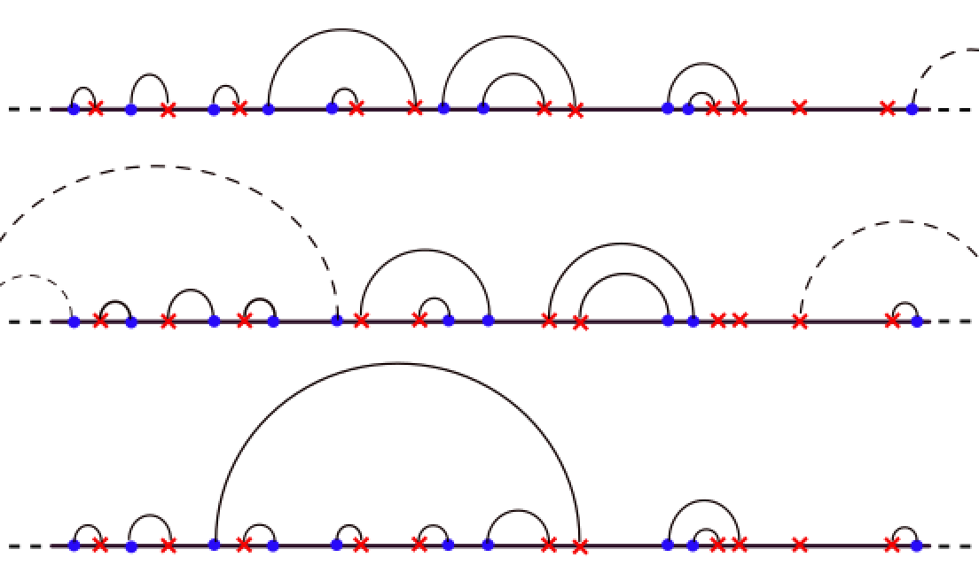
Figure 1. Different matchings between two point processes. Top: forward queue matching $\mathcal{M}_{s}^{+}$, Middle: backward queue matching $\mathcal{M}_{s}^{-}$, Bottom: stable matching $\mathcal{M}_{s}$.

The following are well-known facts about LCFS-PR queues with rate $\lambda$ Poisson arrivals and rate $\mu>\lambda$ i.i.d. exponential service times which are independent of the arrival process. Since $\lambda<\mu$, the queue is stable and each blue point in $\mathcal{B}$ almost surely has a partner in $\mathcal{R}$. Let $x\in\mathcal{B}$ be an arbitrary blue point and let $X^{+}$ be $x$’s matching distance in $\mathcal{M}_{s}^{+}$. It is clear that $X^{+}$ has the same distribution as the busy cycle in the corresponding LCFS-PR queue, where the busy cycle is the duration of time from the arrival of a job at an empty queue to the time the job leaves the queue. It is known (gross1998fundamentals) that the probability density function of the busy cycle is given by

$$f_{\lambda,\mu}(t)=\frac{1}{t\sqrt{\rho}}e^{(\lambda+\mu)t}I_{1}(2t\sqrt{\lambda\mu}),\quad t>0,$$

where $\rho=\frac{\lambda}{\mu}$, and $I_{1}$ is the modified Bessel function of the first kind. Let $B(\lambda,\mu)$ represent this distribution. The average busy cycle duration is $\mathop{\mathbb{E}{}}(X^{+})=1/(\mu-\lambda)$. In the following section we introduce a class of matchings which includes both stable and queue matchings.

4.2. Nested Matching

For any interval $I\in\mathbb{R}$, represent its closure by $\bar{I}$. A matching $\mathcal{M}$ is said to be nested if for any $x,y\in\mathcal{S}$, $x\in I_{\mathcal{M}}(y)$ implies $\mathcal{M}(x)\in\overline{I}_{\mathcal{M}}(y)$. Therefore, in any nested matching if $I_{\mathcal{M}}(x)\cap I_{\mathcal{M}}(y)\neq\emptyset$, then one of the matching segments is nested inside the other one.

Remark. Since the matching segment of an unmatched point $x$ is $(x,\infty)$, there is no matching segment of a matched point in a nested matching which contains an unmatched point.

From the discussion in the previous section it is easy to see that any queue matching is nested. The following lemma proves that the stable matching $\mathcal{M}_{s}$ is also nested.

Lemma 4.2.

The stable matching $\mathcal{M}_{s}$ is nested.

Proof.

See appendix LABEL:stableisnestedproof. ∎

Let $\mathcal{A}$ be the set of all nested matchings between points in $\mathcal{B}$ and $\mathcal{R}$. We say a red point $r$ is a potential match for a blue point $b$, if there exists a nested matching in which $b$ is matched to $r$. For any blue point $b\in\mathcal{B}$ define $\mathcal{P}(b)$ to be the set of all potential matches of $b$,

$$\mathcal{P}(b)=\{r\in\mathcal{R}:\exists\mathcal{M}\in\mathcal{A}\text{~{}s.t.~{}}\mathcal{M}(b)=r\}.$$

The following lemma shows that the set of potential matches of any two blue points are either disjoint or the same.

Lemma 4.3.

For any $b_{1},b_{2}\in\mathcal{B}$, $\mathcal{P}(b_{1})\cap\mathcal{P}(b_{2})\neq\emptyset$ implies $\mathcal{P}(b_{1})=\mathcal{P}(b_{2})$.

Proof.

See appendix LABEL:continuousproofs. ∎

Now define the relation $\sim$ on points in $\mathcal{B}$ as follow:

$$b_{1}\sim b_{2}\Longleftrightarrow\mathcal{P}(b_{1})\cap\mathcal{P}(b_{2})\neq\emptyset.$$

According to Lemma 4.3, for any $b_{1},b_{2}\in\mathcal{B}$, if $\mathcal{P}(b_{1})$ and $\mathcal{P}(b_{2})$ are not disjoint, then they are the same. Therefore, $\sim$ is an equivalence relation on $\mathcal{B}$. For any blue point $b\in\mathcal{B}$, define $[b]$ to be $b$’s equivalence class in $\mathcal{B}$, i.e.,

$$[b]\triangleq\{b^{\prime}\in\mathcal{B}:\mathcal{P}(b^{\prime})=\mathcal{P}(b)\}.$$

Let $N(b)$ represent the size of $b^{\prime}s$ equivalence class, i.e., $N(b)=|[b]|$. Also define $N^{+}(b)=|\{b^{\prime}\in[b],b^{\prime}\geq b\}|$ and $N^{-}(b)=|\{b^{\prime}\in[b],b^{\prime}\leq b\}|$. It is clear that $N(b)=N^{+}(b)+N^{-}(b)-1$. In the following lemma we prove some facts about the structure of the equivalence classes.

Lemma 4.4.

Suppose $\lambda<\mu$ and let $\mathcal{B}$ and $\mathcal{R}$ represent the set of blue and red points in a Poisson matching problem $PM(\lambda,\mu)$, respectively. For any given blue point $b\in\mathcal{B}$ we have

1. there exist $r_{1},r_{2}\in\mathcal{P}(b)$ such that $r_{1}>b$ and $r_{2}<b$, almost surely;

2. there exists exactly one potential red point $r\in\mathcal{P}(b)$ between every two consecutive blue points in $[b]$;

3. $|\mathcal{P}(b)|=N(b)+1$ on $\{|\mathcal{P}(b)|<\infty\}$; and

4. $N^{+}(b)$ and $N^{-}(b)$ are independent geometric random variables with parameter $1-\lambda/\mu$.

Proof.

See appendix LABEL:third. ∎

Let $b\in\mathcal{B}$ be an arbitrary blue point. Since $\lambda<\mu$, then almost surely $|\mathcal{P}(b)|<\infty$. From Lemma 4.4, we can conclude that blue and red points in $[b]\cup\mathcal{P}(b)$ form a finite sequence $\{w_{i}\}$, for $-2N^{-}(b)+1\leq i\leq 2N^{+}(b)-1$, where $b_{0}=b$, $[b]=\{w_{i}:i\text{~{}is even}\}$, and $\mathcal{P}(b)=\{w_{i}:i\text{~{}is odd}\}$. In other words, this sequence starts with a potential red point, alternates between points in $[b]$ and $\mathcal{P}(b)$, and ends with another potential red point. We call the sequence $\{w_{i}\}$ $b$’s potential wave and denote it by $\mathcal{W}(b)$. Figure $2$ shows potential waves of an instance of $PM(\lambda,\mu)$. A key observation here is that in any nested matching, any blue point in $[b]$ should be matched to a red point in $\mathcal{P}(b)$. Therefore, a nested matching first partitions $\mathcal{S}$ into potential waves and then matches points within each wave, separately. In the following section we present our results on the analysis of the matching distance $X$ in the stable matching $\mathcal{M}_{s}$.

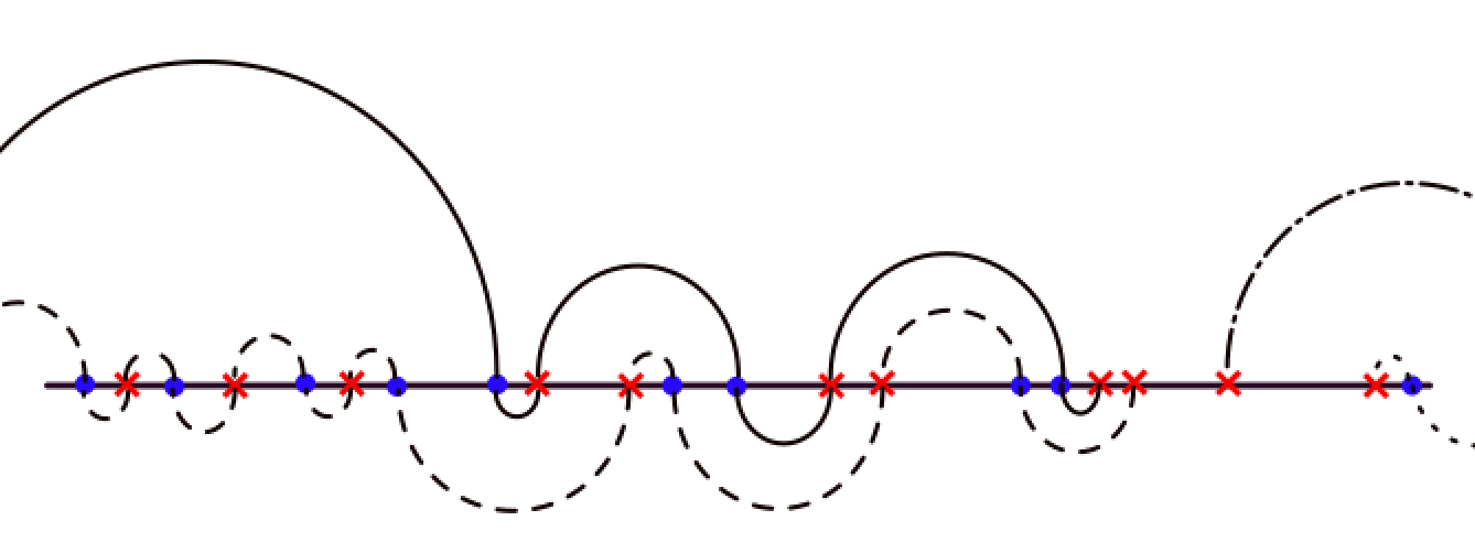
Figure 2. Different potential waves of a sample problem.

4.3. Matching distance, $X$

The following theorem, proves bounds on the distribution of $X$, in terms of busy cycles.

Theorem 4.5.

Consider an instance of a Poisson matching problem $PM(\lambda,\mu)$, where $\lambda<\mu$. Then we have

$$\min\{B_{1},B_{1}^{\prime}\}<X<\max\left\{\sum_{i=1}^{2N-1}B_{i},\sum_{i=1}^{2N^{\prime}-1}B_{i}^{\prime}\right\}$$

where $B_{i}$ and $B_{i}^{\prime}$ are i.i.d. random variables with distribution $B(\lambda,\mu)$, and $N$ and $N^{\prime}$ are i.i.d. geometric random variables with parameter $1-{\lambda}/{\mu}$.

Proof.

See appendix LABEL:boundproof. ∎

Using Theorem 4.5 we can find the following upper bound for the expected matching distance $\mathop{\mathbb{E}{}}(X)$.

Corollary 4.6.

$$\mathbb{E}(X)\leq\left(1+\frac{\mu+\lambda}{\mu-\lambda}\right)\frac{1}{\mu-\lambda}.$$

Proof.

See appendix LABEL:upperboundproof ∎

Remark. Note that the results of Theorem 4.5 and Corollary 4.6 also hold if $X$ is the matching distance in any nested matching.

In the next theorem we improve the upper bound given in Corollary 4.6 for the expected matching distance $\mathop{\mathbb{E}{}}(X)$. The proof of this theorem is extensive and requires some detailed combinatorial arguments. For more details see appendix LABEL:forth.

Theorem 4.7.

For the stable matching $\mathcal{M}_{s}$, we have

$$\mathbb{E}(X)\leq\left(1+\ln\bigl{(}\frac{\mu+\lambda}{\mu-\lambda}\bigr{)}\right)\frac{1}{\mu-\lambda}.$$

Proof.

See appendix LABEL:forth. ∎

In order to evaluate the goodness of the bound in Theorem 4.7, note that for large values of $\mu$ ($\mu\gg\lambda$), with a high probability, each blue point will be matched to the closest red point to it. Therefore, as $\mu/\lambda\to\infty$, $X$ converges to an exponential distribution with rate $2\mu$ (minimum of two i.i.d. exponentials with rate $\mu$) and $\mathop{\mathbb{E}{}}(X)\sim\frac{1}{2\mu}$. However, from Theorem 4.7, in the limit as $\mu/\lambda\to\infty$, $\mathop{\mathbb{E}{}}(X)$ is upper bounded by $\frac{1}{\mu}$.

5. Conclusion

This paper introduced a model for studying matching markets in which preference lists are drawn according to distances in appropriate metric spaces, either between the profiles of participants or between the participants themselves. The model naturally captures several aspects of real world matching markets. Various results regarding the uniqueness and quality of stable matchings were obtained. Specifically, for matchings on the hypercube under the Hamming and Weighted Hamming distances, lower and upper bounds were obtained on the dimension of the hypercube (equal to the number of questions a participant in a dating site needs to answer) so as to obtain unique stable partners or stable matchings. Furthermore, bounds on the distribution and the average value of the matching distance of a typical participant (a measure of the quality of the stable matching) were obtained for stable matchings on the hypercube and on the real line.

We view this work as a first step in studying matching markets in the metric space setting. Several obvious next steps suggest themselves, notably studying the problem under dynamic inputs; i.e., as participants arrive and depart.

Appendix A Appendix

A.1. Proofs omitted from section 3

Proof of Lemma 3.1: Assume, by contradiction, that there exist stable matchings $\mu_{1}$ and $\mu_{2}$ so that for some $z\in\mathcal{S}$, $r_{1}=d_{\mu_{1}}(z)>d_{\mu_{2}}(z)=r_{2}$. Let $r=(r_{1}+r_{2})/2$. For each $x\in\mathcal{S}$, let $P^{\prime}_{x}=\{y\in P_{x}:d(x,y)\leq r\}$ be the preference list $P_{x}$ truncated to contain only those participants who are at a distance less or equal to $r$ from $x$. Let the ordering in the truncated list $P^{\prime}_{x}$ be denoted by $\succ_{x}^{\prime}$. Call the PMP restricted to the truncated preference lists as the “truncated matching problem”. In the truncated matching problem, each person prefers to remain unmatched than to match with a person at a distance greater than $r$ from them. Let $\mu$ be a stable matching for the PMP which has stable partners with a matching distance greater than $r$. Construct the partial matching $\mu^{\prime}$ from $\mu$ by removing all pairs with a distance greater than $r$. We show that $\mu^{\prime}$ is a stable matching for the truncated matching problem. Suppose $m$ and $w$ are not matched to each other in $\mu^{\prime}$. If $d(m,w)>r$, then clearly $(m,w)$ cannot form a blocking pair for the truncated matching problem. Suppose $d(m,w)\leq r$. Since $m$ and $w$ are not matched to each other in $\mu^{\prime}$, they cannot be matched to each other in $\mu$. Moreover, since $\mu$ is stable, either $\mu(m)\succ_{m}w$, or $\mu(w)\succ_{w}m$. Without loss of generality, assume $\mu(m)\succ_{m}w$. Therefore,

$$d\bigl{(}m,\mu(m)\bigr{)}\leq d(m,w)\leq r\Rightarrow\mu(m)\succ_{m}^{\prime}w.$$

This implies $m$ is also matched to $\mu(m)$ in $\mu^{\prime}$; i.e., $\mu^{\prime}(m)=\mu(m)$. Therefore, $\mu^{\prime}(m)\succ_{m}^{\prime}w$ and $(m,w)$ cannot be a blocking pair for $\mu^{\prime}$. This proves that $\mu^{\prime}$ is a stable matching for the truncated matching problem. Now define $S_{r}(\mu)$ to be the set of all users who are matched to someone at a distance greater than $r$ in $\mu$,

$$S_{r}(\mu)\overset{\Delta}{=}\left\{x\in S:d_{\mu}(x)>r\right\}.$$

It is clear that $S_{r}(\mu)$ is the same set of users who are not matched in $\mu^{\prime}$. By the Rural Hospital Theorem, the set of unmatched men and women in the truncated matching problem is the same in all stable matchings. This implies $\mathcal{S}_{r}(\mu)$ does not depend on $\mu$. This contradicts our initial assumption, since $z\in\mathcal{S}_{r}(\mu_{2})$ but $z\notin\mathcal{S}_{r}(\mu_{1})$, proving the lemma. ∎

Consider the RPMP-$k$. Let $\mathcal{M}$ and $\mathcal{W}$ represent the set of $n$ men and $n$ women, respectively. For any profile $\mathbf{a}=(a_{1},...,a_{k})\in Q_{k}$, let $\mathcal{M}_{\mathbf{a}}$ and $\mathcal{W}_{\mathbf{a}}$ be the sets of all men and women whose profiles equal $\mathbf{a}$, respectively. Define $\mathcal{S}_{\mathbf{a}}=\mathcal{M}_{\mathbf{a}}\cup\mathcal{W}_{\mathbf{a}}$.

Lemma A.1.

Fix $\mathbf{a}\in Q_{k}$ and without loss of generality assume $|\mathcal{M}_{\mathbf{a}}|\leq|\mathcal{W}_{\mathbf{a}}|$. We claim that in every stable matching, each man in $\mathcal{M}_{\mathbf{a}}$ will be matched to a woman in $\mathcal{W}_{\mathbf{a}}$.

Proof.

Suppose to the contrary that there is a stable matching $\mu$ and an $m\in\mathcal{M}_{\mathbf{a}}$ such that $\mu(m)\notin\mathcal{W}_{\mathbf{a}}$. Since $|\mathcal{M}_{\mathbf{a}}|\leq|\mathcal{W}_{\mathbf{a}}|$, there should also exist a woman $w\in\mathcal{W}_{\mathbf{a}}$ such that $\mu(w)\notin\mathcal{M}_{\mathbf{a}}$. However, since $d(m,w)=0$, $w\succ_{m}\mu(m)$ and $m\succ_{w}\mu(w)$. Therefore, $(m,w)$ forms a blocking pair for $\mu$, which is a contradiction. ∎

Thus, for any $\mathbf{a}\in Q_{k}$, every stable matching should first try to match men in $\mathcal{M}_{\mathbf{a}}$ with women in $\mathcal{W}_{\mathbf{a}}$ according to their tie-breaking preference lists. Any one unmatched woman in $|\mathcal{W}_{\mathbf{a}}|$ will be matched to someone at a further distance. Define $\mathcal{U}_{\mathbf{a}}$ to be the set of all users with profile $\mathbf{a}$, which are matched to someone with a profile different from $\mathbf{a}$. Note that according to the Rural Hospital Theorem, $\mathcal{U}_{\mathbf{a}}$ is the same for all stable matchings and $|\mathcal{U}_{\mathbf{a}}|=\big{|}|\mathcal{M}_{\mathbf{a}}|-|\mathcal{W}_{\mathbf{a}}|\big{|}$. Define $\mathcal{S}_{\mathbf{a}}=\mathcal{M}_{\mathbf{a}}\cup\mathcal{W}_{\mathbf{a}}$. The following lemma shows that if $k$ is constant, then for any $\mathbf{a}\in Q_{k}$, $|\mathcal{U}_{\mathbf{a}}|=O(\sqrt{n})$.

Lemma A.2.

For any arbitrary profile $\mathbf{a}\in Q_{k}$, as $n\to\infty$,

$$\frac{|\mathcal{M}_{\mathbf{a}}|-|\mathcal{W}_{\mathbf{a}}|}{\sqrt{2p(1-p)n}}\xrightarrow{~{}d~{}}Z_{1}\quad\text{and}\quad\frac{|\mathcal{S}_{\mathbf{a}}|-2np}{\sqrt{2p(1-p)n}}\xrightarrow{~{}d~{}}Z_{2},$$

where $p=2^{-k}$, $Z_{1}$ and $Z_{2}$ are independent standard normal–$\mathcal{N}(0,1)$–random variables, and $\xrightarrow{~{}d~{}}$ represents convergence in distribution.

Proof.

First note that $|\mathcal{M}_{\mathbf{a}}|$ and $|\mathcal{W}_{\mathbf{a}}|$ are i.i.d. with a Binomial$(n,p)$ distribution. From Central Limit Theorem (CLT) we have that as $n\to\infty$,

$$\frac{|\mathcal{M}_{\mathbf{a}}|-np}{\sqrt{np(1-p)}}\xrightarrow{~{}d~{}}{N}_{1},\quad\frac{|\mathcal{W}_{\mathbf{a}}|-np}{\sqrt{np(1-p)}}\xrightarrow{~{}d~{}}{N}_{2},$$

where $N_{1}$ and $N_{2}$ are two independent random variables with a standard normal distribution, i.e., $N_{1},N_{2}\sim\mathcal{N}(0,1)$. Therefore, as $n\to\infty$,

$$\frac{|\mathcal{M}_{\mathbf{a}}|-|\mathcal{W}_{\mathbf{a}}|}{\sqrt{2p(1-p)n}}\xrightarrow{~{}d~{}}\frac{N_{1}-N_{2}}{\sqrt{2}},\quad\frac{|\mathcal{S}_{\mathbf{a}}|-2np}{\sqrt{2p(1-p)n}}\xrightarrow{~{}d~{}}\frac{N_{1}+N_{2}}{\sqrt{2}}.$$

Define $Z_{1}=({N_{1}-N_{2}})/{\sqrt{2}}$ and $Z_{2}=(N_{1}+N_{2})/{\sqrt{2}}$. It is clear that $Z_{1},Z_{2}\sim\mathcal{N}(0,1)$. Moreover, since $N_{1}$ and $N_{2}$ are independent, $Z_{1}$ and $Z_{2}$ are also independent. This completes the proof. ∎

Since Lemma A.1 requires each stable matching $\mu$ to first match men and women in $\mathcal{S}_{\mathbf{a}}$ using their tie-breaking preference lists, the $O(\sqrt{n})$ discrepancy between the number of men and women in $\mathcal{S}_{\mathbf{a}}$ makes this sub-problem significantly unbalanced. Using the approach of ashlagi2014unbalanced, we prove some useful bounds on the number of stable partners in unbalanced matching problems which is true for every $n$.

Lemma A.3.

Let $r\geq 1$ and consider an unbalanced two-sided matching problem with $n$ men and $n+r$ women represented by $\mathcal{M}$ and $\mathcal{W}$, respectively. Suppose the men’s preference lists are generated independently and uniformly at random from the set of all orderings of women in $\mathcal{W}$. Similarly, suppose the women’s preference lists are generated independently and uniformly at random from the set of all orderings of men in $\mathcal{M}$. For any given $x\in\mathcal{M}\cup\mathcal{W}$, let $N(x)$ represent the number of $x$’s stable partners. We have that

$$\mathop{\mathbb{P}}\big{(}N(x)>1\big{)}\leq\frac{1}{r+1}\quad\text{and}\quad\mathop{\mathbb{E}{}}\big{(}N(x)\big{)}\leq 1+\frac{1}{r}.$$

Proof.

Let $\mu_{\mathcal{M}}$ represent the men-optimal stable matching found by running the men-proposing deferred acceptance algorithm, and let $U$ be the set of all women who are not matched in $\mu_{\mathcal{M}}$. According to the Rural Hospital Theorem, the set of women who are unmatched is the same as $U$ for all stable matchings. Let $w\in\mathcal{W}\backslash U$ be an arbitrary woman. In order to find all the stable partners of $w$, we employ the same algorithm that is used in mcvitie1970stable, immorlica2005marriage, and ashlagi2014unbalanced. It has been proved by immorlica2005marriage that the following algorithm outputs all the stable partners of $w$.

Algorithm I

1. Run the men-proposing algorithm to find the men-optimal stable matching $\mu_{\mathcal{M}}$. If $w$ is unmatched in $\mu_{\mathcal{M}}$, output $\emptyset$. Initialze $\mu=\mu_{\mathcal{M}}$ .

2. Set $m=\mu(w)$ and output $m$ as one of the stable partners of $w$. Then have $w$ reject $m$ and remove the pair $(m,w)$ from $\mu$. Set $u=m$. ($u$ represents the current unmatched man.)

3. Let $w^{\prime}$ be the next woman in $u$’s preference list whom he has not proposed to yet. If $w^{\prime}$ is unmatched in $\mu_{\mathcal{M}}$, terminate the algorithm.

4. 1. If $w^{\prime}$ has already received a proposal from someone better than, she simply rejects $u$ and the algorithm continues to step $3$.

   2. If not, $w^{\prime}$ accepts $u$’s proposal. If $w=w^{\prime}$, the algorithm continues to step $2$. Otherwise, set $u=\mu(m^{\prime})$ and the algorithm continues to step $3$.

In order to analyze algorithm I, we use the principle of deferred decision which assumes that the random preference lists are not known in advance and rather unfold step by step in the algorithms when a proposal/rejection happens. Let $t_{i}$ be the time of the $i^{\text{t}h}$ visit of the algorithm at step $3$, and define $u_{i}$ and $w_{i}^{\prime}$ to be the unmatched man and the next woman who $u_{i}$ wants to propose to at time $t_{i}$. Also define $X_{i}$ to be the set of all women who $u_{i}$ has not proposed to yet at time $t_{i}$. Since we are using the principle of deferred decision, at any time $t_{i}$, rankings of women in $X_{i}$ are not yet unfolded in $u_{i}$’s preference list. Therefore, at any time $t_{i}$, every woman in $X_{i}$ has the same chance of ${1}/{|X_{i}|}$ to receive the next proposal from $u_{i}$. Define the events $E_{i}=\left\{w_{i}^{\prime}\in\{w\}\cup U\right\}$. Since the algorithm has not been terminated by time $t_{i}$, $U\subseteq X_{i}$. Therefore, given $E_{i}$, the probability that $u_{i}$ proposes to $w$ is at most $1/(r+1)$, and the probability that the algorithm terminates is at least $r/(r+1)$, i.e.  ,

$$\mathop{\mathbb{P}}(w_{i}^{\prime}=w~{}|~{}E_{i})\leq\frac{1}{r+1},$$

and

$$\mathop{\mathbb{P}}(\text{The algorithm terminates at~{}}t_{i}~{}|~{}E_{i})\geq\frac{r}{r+1}.$$

As the algorithm progresses, woman $w$ finds a new stable partner only if she receives a proposal from an unmatched man at step $3$ of the algorithm. Let $V_{i}$ be the total number of proposals received by woman $w$ from time $t_{1}$ to time $t_{i}$. If $E_{i}$ does not occur then $V_{i+1}=V_{i}$, and if $E_{i}$ occurs then $V_{i+1}=V_{i}+1$ with a probability of at most $1/(r+1)$ and the algorithm terminates with a probability at least $r/(r+1)$. Therefore, if $V$ represents the total number of proposals received by $w$ after time $t_{1}$, V is stochastically dominated by a geometric random variable with rate $p=r/(r+1)$. Thus,

$$\mathop{\mathbb{P}}(V>0)\leq\frac{1}{r+1},$$

and

$$\mathop{\mathbb{E}{}}(V)\leq\frac{1-p}{p}=\frac{1}{r}.$$

Since $\mathcal{N}(w)\leq 1+V$, the proof is complete for any $w\in\mathcal{W}$. It remains to prove the inequalities for $x\in\mathcal{M}$. Fix $x\in\mathcal{M}$. Note that the two events $\{\mathcal{N}(x)>1\}$ and $\{\mathcal{N}(\mu_{\mathcal{M}}(x))>1\}$ are equivalent. Therefore, Since $\mu_{\mathcal{M}}(x)\in\mathcal{W}$,

$$\mathop{\mathbb{P}}\big{(}\mathcal{N}(x)>1\big{)}=\mathop{\mathbb{P}}\big{(}\mathcal{N}(\mu_{\mathcal{M}}(x))>1\big{)}\leq\frac{1}{r+1}.$$

Moreover, since $\sum_{m\in\mathcal{M}}\mathcal{N}(m)=\sum_{w\in\mathcal{W}\backslash U}\mathcal{N}(w)$ (both are equal to the total number of stable partner pairs), from symmetry we have,

$$\mathop{\mathbb{E}{}}\left(N(x)\right)=\frac{1}{n}\sum_{m\in\mathcal{M}}\mathop{\mathbb{E}{}}\left(\mathcal{N}(m)\right)=\frac{1}{n}\sum_{w\in\mathcal{W}\backslash U}\mathop{\mathbb{E}{}}\left(\mathcal{N}(w)\right)\leq 1+\frac{1}{r}.$$

∎

We now prove Theorem 3.2 by using Lemmas A.2 and A.3.

Proof of Theorem 3.2: Part (i). We prove this part of the theorem only for constant profile size $k\geq 1$. The proof for arbitrary profile size $k\leq(1-\epsilon)\log n$ is similar. Fix $n$ and consider an instance of the random profile matching problem with $n$ men and $n$ women represented by $\mathcal{M}^{(n)}$ and $\mathcal{W}^{(n)}$, respectively. Let $x\in\mathcal{M}^{(n)}\cup\mathcal{W}^{(n)}$ be an arbitrary user and let $\mathbf{a}\in Q_{k}$ represent his/her profile. Define $\mathcal{M}_{\mathbf{a}}^{(n)}$, $\mathcal{W}_{\mathbf{a}}^{(n)}$, and $\mathcal{S}_{\mathbf{a}}^{(n)}$ as before. Also define $Z_{1}^{(n)}={(|\mathcal{S}_{\mathbf{a}}^{(n)}|-2np)}/{\sqrt{2np(1-p)}}$ and $Z_{2}^{(n)}={(|\mathcal{W}_{\mathbf{a}}^{(n)}|-|\mathcal{M}_{\mathbf{a}}^{(n)}|)}/{\sqrt{2np(1-p)}}$. According to Lemma A.2, as $n\to\infty$, $Z_{1}^{(n)}\xrightarrow{~{}d~{}}Z_{1}$ and $Z_{2}^{(n)}\xrightarrow{~{}d~{}}Z_{2}$, where $Z_{1},Z_{2}\sim\mathcal{N}(0,1)$, and $Z_{1}$ and $Z_{2}$ are independent. For any $\epsilon>0$ define subsets $A_{\epsilon},B_{\epsilon}\subseteq\mathbb{R}$ as follows,

$$A_{\epsilon}=[-\infty,-\frac{1}{\epsilon}]\cup[\frac{1}{\epsilon},+\infty],\quad B_{\epsilon}=[0,\epsilon]\cup[\frac{1}{\epsilon},+\infty].$$

Let $\delta>0$ be an arbitrary positive number. Choose $\epsilon>0$ small enough to have, ${\mathop{\mathbb{P}}}\left(Z_{1}\in A_{\epsilon}\right)\leq\frac{\delta}{8}$ and ${\mathop{\mathbb{P}}}\left(|Z_{2}|\in B_{\epsilon}\right)\leq\frac{\delta}{8}$. Since $Z_{1}^{(n)}$ and $Z_{2}^{(n)}$ converge in distribution to $Z_{1}$ and $Z_{2}$, respectively, there exists a large number $N_{1}$ such that for any $n>N_{1}$,

$$\bigl{|}\mathop{\mathbb{P}}(Z_{1}\in A_{\epsilon})-\mathop{\mathbb{P}}(Z_{1}^{(n)}\in A_{\epsilon})\bigr{|}<\frac{\delta}{8},\quad\bigl{|}\mathop{\mathbb{P}}(Z_{2}\in B_{\epsilon})-\mathop{\mathbb{P}}(Z_{2}^{(n)}\in B_{\epsilon})\bigr{|}<\frac{\delta}{8}.$$

Therefore, for any $n>N_{1}$ we have,

$$\mathop{\mathbb{P}}\left(Z_{1}^{(n)}\in A_{\epsilon}\text{~{}~{}or~{}~{}}Z_{2}^{(n)}\in B_{\epsilon}\right) \leq\mathop{\mathbb{P}}(Z_{1}^{(n)}\in A_{\epsilon})+\mathbb{P}(Z_{2}^{(n)}\in B_{\epsilon})$$

$$\leq{\mathop{\mathbb{P}}}(Z_{1}\in A_{\epsilon})+\bigl{|}\mathop{\mathbb{P}}(Z_{1}^{(n)}\in A_{\epsilon})-\mathop{\mathbb{P}}(Z_{1}\in A_{\epsilon})\bigr{|}$$

$$+{\mathop{\mathbb{P}}}(Z_{2}\in B_{\epsilon})+\bigl{|}\mathop{\mathbb{P}}(Z_{2}^{(n)}\in B_{\epsilon})-\mathop{\mathbb{P}}(Z_{2}\in B_{\epsilon})\bigr{|}$$

$$\leq\frac{\delta}{2}.$$

Therefore, with a probability of at least $1-{\delta}/{2}$, the following event occurs:

$$E=\Big{\{}|\mathcal{S}_{\mathbf{a}}^{(n)}|\in[2np-C_{1}\sqrt{n},2np+C_{1}\sqrt{n}]\text{~{}~{}and~{}~{}}\big{|}|\mathcal{W}_{\mathbf{a}}^{(n)}|-|\mathcal{M}_{\mathbf{a}}^{(n)}|\big{|}\in[C_{2}\sqrt{n},C_{3}\sqrt{n}]\Big{\}},$$

where $C_{1}=\frac{\sqrt{2p(1-p)}}{\epsilon}$, $C_{2}=\epsilon\sqrt{p(1-p)}$, and $C_{3}=\frac{\sqrt{p(1-p)}}{\epsilon}$. Without loss of generality assume $|\mathcal{M}_{\mathbf{a}}^{(n)}|\leq|\mathcal{W}_{\mathbf{a}}^{(n)}|$ and define $r=|\mathcal{W}_{\mathbf{a}}^{(n)}|-|\mathcal{M}_{\mathbf{a}}^{(n)}|$. The problem of matching men in $\mathcal{M}_{\mathbf{a}}^{(n)}$ and women in $\mathcal{W}_{\mathbf{a}}^{(n)}$ according to preference lists given by $\succ^{P}$ is an unbalanced matching problem with a discrepancy equal to $r$ between the number of men and the number of women. Let $\mathcal{U}_{a}^{(n)}$ represent the set of unmatched women in the men-optimal stable matching for this unbalanced matching problem. Therefore, if $N^{(n)}(x)$ represents the number of $x$’s stable partners, we have,

$${\mathop{\mathbb{P}}}\big{(}N^{(n)}(x)>1\big{)} \leq{\mathop{\mathbb{P}}}{(}E^{o}{)}+{\mathop{\mathbb{P}}}\big{(}N^{(n)}(x)>1\big{|}E\big{)}$$

$$={\mathop{\mathbb{P}}}{(}E^{o}{)}+{\mathop{\mathbb{P}}}\big{(}x\in\mathcal{U}_{a}^{(n)}\big{|}E\big{)}+{\mathop{\mathbb{P}}}\big{(}N^{(n)}(x)>1\big{|}E,x\notin\mathcal{U}_{a}^{(n)}\big{)}$$

$$\leq{\mathop{\mathbb{P}}}{(}E^{o}{)}+\frac{r}{|\mathcal{S}_{\mathbf{a}}^{(n)}|}+\frac{1}{r+1}$$

$$\leq\frac{\delta}{2}+\frac{C_{2}\sqrt{n}}{2np-C_{1}\sqrt{n}}+\frac{1}{C_{1}\sqrt{n}+1},$$

where in the first inequality we used the results of the Lemma A.3, and in the last inequality we used the bounds on $r$ and $|\mathcal{S}_{\mathbf{a}}^{(n)}|$ given by the event $E$. Pick $N_{2}$ large enough to have,

$$\frac{C_{2}\sqrt{n}}{2np-C_{1}\sqrt{n}}+\frac{1}{C_{1}\sqrt{n}+1}<{\delta}/{2},\quad\forall n\geq N_{2}.$$

Define $N=\max\{N_{1},N_{2}\}$. Therefore, for any $n>N$, ${\mathop{\mathbb{P}}}\big{(}N^{(n)}(x)>1\big{)}\leq\delta$. Since $\delta>0$ is arbitrary,

$$\mathop{\mathbb{P}}\big{(}N^{(n)}(x)=1\big{)}\to 1\text{~{}~{}as~{}~{} }n\to\infty.$$

This implies that with high probability the fraction of users with multiple stable partners tends to zero as $n\to\infty$.
Part (ii). In order to prove the second part of the theorem, note that since $|\mathcal{M}_{\mathbf{a}}|$ and $|\mathcal{W}_{\mathbf{a}}|$ are Binomial random variables with parameters $n$ and $p=2^{-k}=1/n$, according to the well-known Poisson limit theorem, both converge to the Poisson$(1)$ distribution as $n$ goes to infinity. Therefore, in the limit, with a positive probability of $c={e^{-2}}/{4}$ there are exactly two men and two women whose profiles are equal to $\mathbf{a}$. On the other hand, it is easy to see that in a random stable matching problem with two men and two women, the probability of having exactly two stable matchings is equal to $1/8$. Therefore, for any given profile $\mathbf{a}\in Q_{k}$, with a positive probability of $\beta={c}/{8}>0$, there are exactly two men and two women with profile $\mathbf{a}$ who have multiple stable partners. This proves that the expected number of users with multiple stable partners is $O(n)$. Moreover, since the number of such profiles is $O(n)$, in expectation there are exponentially many stable matchings. ∎
The following lemma shows that if the preference list of a user is uniquely identified by profile distances and no further tie-breaking is required, then he/she has a unique stable partner.

Lemma A.4.

In a profile matching problem, if the distances of a given user $x$ from all the members of the opposite sex are distinct, then $x$ has a unique stable partner.

Proof.

By contradiction, suppose $x$ has two different stable partners $y_{1}$ and $y_{2}$. According to Lemma 3.1, $y_{1}$ and $y_{2}$ should be at the same distance from $x$. But, this contradicts with the assumption that $x$ has different distances from $y_{1}$ and $y_{2}$. Therefore, $x$ has a unique stable partner. ∎

In order to apply Lemma A.4, $k$ should be large enough to have a unique stable matching without resorting to tie-breaks. Now we prove Theorems 3.3 and 3.4.

Proof of Theorem 3.3: Part (i). Let $x$ be an arbitrary user and without loss of generality, assume $x\in\mathcal{W}$. Suppose $x$ has multiple stable partners and let $y$ and $y^{\prime}$ be two different stable partners of $x$. Since $x$ has multiple sable partners, $y$ also has another stable partner $x^{\prime}$ (different from $x$). According to Lemma 3.1, $d_{h}(x,y^{\prime})=d_{h}(x,y)=d_{h}(x^{\prime},y)$. For any $z\in\mathcal{M}$ define the following event

$$E_{z}=\bigl{\{}\exists x^{\prime}\in\mathcal{W}\backslash\{x\},\exists z^{\prime}\in\mathcal{M}\backslash\{z\};d_{h}(x,z^{\prime})=d_{h}(x,z)=d_{h}(x^{\prime},z)\bigr{\}}.$$

Using the union bound we have,

$$\mathop{\mathbb{P}}(E_{z}) =\mathop{\mathbb{P}}\Bigl{(}\exists x^{\prime}\in\mathcal{W}\backslash\{x\};d_{h}(x,z)=d_{h}(x^{\prime},z)\Bigr{)}\mathop{\mathbb{P}}\Bigl{(}\exists z^{\prime}\in\mathcal{M}\backslash\{z\};d_{h}(x,z)=d_{h}(x,z^{\prime})\Bigr{)}$$

$$\leq\Bigl{(}(n-1)\mathop{\mathbb{P}}\bigl{(}d_{h}(x,m)=d_{h}(x,z)\bigr{)}\Bigr{)}\Bigl{(}(n-1)\mathop{\mathbb{P}}\bigl{(}d_{h}(w,z)=d_{h}(x,z)\bigr{)}\Bigr{)}$$

$$\leq n^{2}\mathop{\mathbb{P}}\bigl{(}d_{h}(x,m)=d_{h}(x,z)\bigr{)}^{2}$$

where $m$ and $w$ are a man and a woman who are chosen randomly from $\mathcal{M}$ and $\mathcal{W}$, respectively. Note that in the last inequality we used the existing symmetry in the problem. Since $d_{h}(x,m)$ has a binomial distribution (as a function of the random variable $m$), the maximum value of $\mathop{\mathbb{P}}\bigl{(}d_{h}(x,m)=d_{h}(x,z)\bigr{)}$ is at $d_{h}(x,z)=\lfloor k/2\rfloor$. Using the Sterling approximation we have:

$${\mathop{\mathbb{P}}}\bigl{(}d_{h}(x,m)=\frac{k}{2}\bigr{)}=\frac{k!}{\frac{k}{2}!\frac{k}{2}!}2^{-k}\simeq\frac{\sqrt{2\pi k}(\frac{k}{e})^{k}}{\pi k(\frac{k}{2e})^{k}}2^{-k}=\sqrt{\frac{2}{\pi}}\frac{1}{\sqrt{k}}.$$

Therefore,

$$\mathop{\mathbb{P}}(x\text{ has multiple stable partners})\leq\mathop{\mathbb{P}}\left(\cup_{z\in\mathcal{M}}E_{z}\right)\leq n^{3}{\frac{2}{\pi k}}.$$

Since $k=\Omega(n^{3})$, the right hand side of the above inequality tends to zero as $n$ goes to infinity. This implies that with high probability the fraction of users with multiple stable partners tends to zero as $n$ goes to infinity. Note that using the union bound, we can conclude that if $k=\Omega(n^{4})$, with high probability, there exists a unique stable matching.
Part (ii). Fix a woman $x\in\mathcal{W}$. For any $y\in\mathcal{M}$, define the event $E_{y}=\{\exists y^{\prime}\in\mathcal{M}\backslash\{y\};d_{h}(x,y)=d_{h}(x,y^{\prime})\}$. Also define $A_{x}$ to represent the event that the distances of $x$ from all men in $\mathcal{M}$ are distinct. Similar to part (i) we have

$$\mathop{\mathbb{P}}(A_{x}^{c})\leq\mathop{\mathbb{P}}\left(\cup_{y\in\mathcal{M}}E_{y}\right)\leq n^{2}\sqrt{\frac{2}{k\pi}}.$$

According to Lemma A.4, if the event $A_{x}$ happens for every $x\in\mathcal{W}$, there is a unique stable matching without resorting to tie-breaking. Therefore,

$$\mathop{\mathbb{P}}(\text{There are multiple stable matchings}) \leq\mathop{\mathbb{P}}\left(\cup_{x\in\mathcal{W}}A_{x}^{c}\right)\leq n^{3}\sqrt{\frac{2}{k\pi}}.$$

Since $k=\Omega(n^{6})$, the probability that there are multiple stable matchings goes to zero as $n$ goes to infinity.
Part (iii). Without loss of generality assume $x\in\mathcal{W}$ and let $X_{i}$ represent the distance of $x$ from man $m_{i}$, i.e., $d_{i}=d_{h}(x,m_{i})$. Clearly, $X_{i}$’s are i.i.d. with Binomial distribution with parameters $k$ and $1/2$. Define $Z=\min_{i}X_{i}$. Clearly $d_{h}(x)\geq Z$. Therefore, for any positive number $r>0$,

$$\mathop{\mathbb{P}}(d_{h}(x)\geq r)\geq\mathop{\mathbb{P}}(Z\geq r)=\mathop{\mathbb{P}}(\min_{i}X_{i}\geq r)=\prod_{i=1}^{n}\mathop{\mathbb{P}}(X_{i}\geq r)=\mathop{\mathbb{P}}(X_{1}\geq r)^{n}.$$

Now, according to the Chernoff’s inequality,

$$\mathop{\mathbb{P}}(X_{1}<r)\leq e^{-\frac{1}{{k}}{(\frac{k}{2}-r)^{2}}}.$$

Therefore,

$$\mathop{\mathbb{P}}(d_{h}(x)\geq r)\geq(1-e^{-\frac{1}{{k}}{(\frac{k}{2}-r)^{2}}})^{n}\geq 1-ne^{-\frac{1}{{k}}{(\frac{k}{2}-r)^{2}}}.$$

Now if we set $r=k/2-\sqrt{\beta k\log n}$ we have,

$$\mathop{\mathbb{P}}\left(d_{h}(x)\geq k/2-\sqrt{\beta k\log n}\right)\geq 1-n^{1-\beta}.$$

∎

Proof of Theorem 3.4: Part (i). Without loss of generality assume $x\in\mathcal{M}$ and suppose $y$ is a stable partner for $x$. If $x$ has multiple stable partners, then $y$ should also have multiple stable partners. Let $x^{\prime}$ be another stable partner of $y$ different from $x$. According to Lemma 3.1, $x$ and $x^{\prime}$ should have the same distance from $y$. However, in the weighted hamming distance metric, if $d_{w}(\mathbf{a}(y),\mathbf{a}(x))=d_{w}(\mathbf{a}(y),\mathbf{a}(x^{\prime}))$, then $x$ and $x^{\prime}$ should have the exact same profiles, i.e., $\mathbf{a}(x)=\mathbf{a}(x^{\prime})$. Therefore, if a man $x$ has multiple stable partners, there should exist another man $x^{\prime}$ with the same profile as him. However, by using union bounds we get

$$\mathop{\mathbb{P}}\left(\exists x^{\prime}\in\mathcal{M};\mathbf{a}(x^{\prime})=\mathbf{a}(x)\right)\leq(n-1)\frac{1}{2^{k}}\leq n^{-\epsilon}.$$

This proves that the probability that $x$ has multiple stable partners is vanishingly small.
Part (ii). We first show that if there are multiple stable matchings, then there are two men (or women) who have the same profile. If there are multiple stable matchings, there should exists a chain $\{c_{i}\}_{i=0}^{2s-1}$ of men and women such that $c_{i}\in\mathcal{M}$ if $i$ is even, and $c_{i}\in\mathcal{W}$ if $i$ is odd. Moreover, in this chain for every $i\in\{0,\dots,2s-1\}$, $c_{i+1}\succ_{c_{i}}c_{i-1}$ ($i-1$ and $i+1$ are taken in mode $2s$). Define $d_{i}=d_{w}(c_{i},c_{i+1})$, $0\leq i<2s$. Let $j$ be the index at which $d_{i}$ is minimum. Now, if the values of $d_{i}$ are all distinct, then $c_{j}\succ_{c_{j+1}}c_{j+2}$ which is a contradiction. Therefore, There should exist an index $i$ such that, $d_{i}=d_{i+1}$. Following our discussion in part (i), this implies that $c_{i}$ and $c_{i+2}$ should have the same profile. However, the probability that two randomly selected men (or women) have the same profile is $2^{-k}$. Using union bound we can conclude that the probability that there are multiple stable matchings is upper bounded by $n^{2}2^{-k}\leq n^{-\epsilon}$.