Malware Lineage in the Wild

Abstract

Malware lineage studies the evolutionary relationships among malware and has important applications for malware analysis. A persistent limitation of prior malware lineage approaches is to consider every input sample a separate malware version. This is problematic since a majority of malware are packed and the packing process produces many polymorphic variants (i.e., executables with different file hash) of the same malware version. Thus, many samples correspond to the same malware version and it is challenging to identify distinct malware versions from polymorphic variants. This problem does not manifest in prior malware lineage approaches because they work on synthetic malware, malware that are not packed, or packed malware for which unpackers are available.

In this work, we propose a novel malware lineage approach that works on malware samples collected in the wild. Given a set of malware executables from the same family, for which no source code is available and which may be packed, our approach produces a lineage graph where nodes are versions of the family and edges describe the relationships between versions. To enable our malware lineage approach, we propose the first technique to identify the versions of a malware family and a scalable code indexing technique for determining shared functions between any pair of input samples. We have evaluated the accuracy of our approach on $13$ open-source programs and have applied it to produce lineage graphs for 10 popular malware families. Our malware lineage graphs achieve on average a $26$ times reduction from number of input samples to number of versions.

I Introduction

Malware lineage studies the evolutionary relationships among malware, which has important security applications in the context of malware analysis. For example, lineage can be a fundamental step for triage, labeling, categorization, threat intelligence, provenance, and authorship attribution. The goal of malware lineage is to produce a lineage graph where nodes are versions of the family and edges describe the ancestor-descendant relationships between versions.

Similar to benign programs, malware families evolve to adapt to changing requirements by adding new functionality, and to improve stability by fixing bugs. However, malware development typically comprises of an extra step not present in benign software development. Once a new version of a malware family is ready, the malware authors pack the resulting executable to hide its functionality and thus bypass detection by commercial malware detectors. The packing process takes as input an executable and produces another executable with the same functionality. The packing process is typically applied many times to the same input executable, creating polymorphic variants (i.e., executables) of exactly the same version, which look different to malware detectors.

An important open problem in malware lineage is identifying the versions of a malware family among a set of input executables belonging to the family. The study of malware lineage goes back over $20$ years and multiple approaches have been proposed [66, 30, 24, 11, 35, 48, 74, 27, 36, 43, 33, 14]. However, a persistent limitation of these approaches is that they consider every input sample a separate malware version. Thus, their output lineage graphs have a node for every input sample. This is problematic because the packing process produces many polymorphic variants of a malware version. Thus, many input samples should be represented by the same node in the lineage graph. This problem does not manifest in prior malware lineage approaches because they are evaluated on synthetic malware, malware that is not packed, or packed malware for which unpackers are readily available (e.g., UPX [70]). But, the majority of malware is packed and malware often uses custom packers for which off-the-shelf unpackers are not available [68]. Thus, version identification needs to be addressed with malware collected in the wild.

Identifying versions among packed samples from a malware family is a novel and challenging problem. This problem differs from program similarity [22] because two versions of the same family may be highly similar, but still different versions. For example, one version may patch the previous one by adding a conditional to fix an error condition. While the two versions may be nearly identical, they need to be represented by different nodes in the lineage graph. We address this problem by considering malware samples with the same set of functions as polymorphic variants, which should be represented by the same node in the lineage graph. Any changes in functionality between two samples such as adding a function, removing a function, or updating an existing function, means that both samples are from different versions, with their own nodes in the lineage graph.

Another challenge with malware collected in the wild is that we do not know how it was developed. Thus, we need a lineage inference algorithm that works independently of the development model used by the malware authors, e.g., straight-line, multiple independent lines, branching and merging. Unfortunately, iLine [33], the state-of-the-art lineage inference algorithm, uses separate algorithms for straight-line and branching and merging development. Thus, iLine requires knowing in advance the development model of the software to select the lineage algorithm. This is problematic with malware since the development model is not known.

In this work, we propose a novel malware lineage approach that works on malware samples collected in the wild. Given a pool of malware executables from the same family, for which no source code is available and which may be packed with an unknown packer, it produces a lineage graph. Our malware lineage approach improves the state-of-art in two ways. First, we propose the first technique to identify the different versions of a malware family present in an input set of potentially packed executables. In our lineage graph, a node identifies a version of the malware family and represents all input samples that are polymorphic variants of that version, which greatly reduces the number of nodes compared to prior approaches that create one node per input sample. Second, we propose a novel lineage inference algorithm that works independently of the development model used by the malware, and that improves the accuracy compared to iLine, the state-of-the-art lineage inference approach.

Performing lineage inference on malware samples collected in the wild requires addressing other challenges such as malware clustering [6, 57, 32, 60], unpacking [49, 62, 34, 17, 8], and disassembly [41, 44]. To address these challenges we adapt existing state-of-the-art solutions. In other words, our goal is not to propose novel malware clustering, unpacking, and disassembly techniques. Rather, we want to understand how far we can get using state-of-the-art techniques and to identify areas where improvements are needed. To this end, we propose two novel metrics to quantify the accuracy of the malware unpacking and disassembly process.

Our approach works as follows: Since malware executables are collected in the wild without labels indicating their family, we first cluster input executables into malware families. Then, each malware sample is unpacked using a generic dynamic unpacker. The unpacker recovers the original code as raw byte sequences in memory snapshots. To enable malware lineage, we need to represent the code in a form that enables further analysis. For this, we disassemble the unpacked malware code by removing code overlaps, identifying function boundaries, and applying dynamic information to improve disassembly results. This process outputs the unpacked and disassembled code as an IDA database [31], which serves as input to the lineage inference module that produces the lineage graph.

We have implemented our malware lineage approach and evaluated its accuracy on open-source programs, before applying it to 10 malware families. Our unpacking and disassembly modules recover up to 81% of the original functions of programs packed with $18$ packers. The missing functions are properly unpacked, but the function identification misses their start addresses preventing their disassembly. We have evaluated our lineage inference module on 631 versions of $13$ open-source programs, covering over $59$ years of software development. Our lineage graphs achieve an average 95% accuracy, which improves on iLine’s results, without requiring apriori knowledge of the malware development model. We also show that our version identification technique has better accuracy and efficiency compared to using BinDiff.

We have also evaluated our approach on 7,793 packed malware samples from 10 malware families. The generated lineage graphs show that our approach can handle different malware development models, i.e., straight line, $k$ independent lines, branching and merging. The lineage graphs succinctly summarize the evolution of a malware family, achieving an average $26$ times reduction from number of input samples to number of versions. For example, the $1,354$ Sytro samples are grouped into $6$ versions in the Sytro lineage graph.

Our contributions are:

• We propose a novel approach for malware lineage that works with malware collected in the wild. It takes as input a set of samples from the same malware family and outputs a lineage graph that describes ancestor-descendant relationships among the family versions.

• We present the first technique for identifying the versions present in a pool of samples from the same malware family. Our technique classifies the input samples into versions, identifying polymorphic variants of the same version.

• We propose a novel lineage inference algorithm that works independently of the development process used by the malware and that improves the accuracy compared to the current state-of-the-art solution.

• We propose two metrics to quantify the accuracy of the unpacking and disassembly process.

• We evaluate the accuracy of our lineage approach on 13 open-source programs, achieving 95% accuracy on the lineage graphs. We apply our approach to 10 malware families achieving a $26$ times reduction from input samples to versions.

II Overview & Problem Definition

Our problem is given a set of malware samples from the same malware family collected in the wild, to build a lineage graph that captures the evolution of the malware family across versions. Section II-A details the challenges introduced by working on malware collected in the wild. Section II-B details the problem. And, Section II-C describes the version identification subproblem.

II-A Challenges

The main requirement for our malware lineage approach is to handle malware samples collected in the wild. This entails the following challenges:

• Unknown versions. We ignore how many versions a malware family has, i.e., we do not know apriori the nodes in the lineage graph. Instead, we need to identify which input samples correspond to different versions and which are polymorphic variants of the same version. This is a key difference from our approach with respect to prior malware lineage approaches [30, 24, 11, 35, 74, 27, 36, 33, 14] that consider each input sample as a distinct version.

• Unknown development model. We ignore how a malware family is developed. The current state-of-the-art malware lineage approach is iLine [33], which proposes different malware lineage algorithms for different development models, e.g., one for straight-line and another for branching and merging. But, with malware we do not know apriori which development model has been used. By contrast, we propose a single lineage inference algorithm that works regardless of the development model used.

• Unpacking. Malware is distributed as executables, i.e., without source code, and those executables are typically packed. Polymorphic variants are created by repacking the same version multiple times. Our approach unpacks the input malware executables to recover the original code.

• Disassembly. Malware disassembly is a difficult problem [41]. Our disassembly module addresses code overlaps, function identification, and uses dynamic information to guide the disassembly. It outputs the unpacked program as an IDA database.

• Unordered samples. The order in which malware samples are collected may not mirror the order in which their versions were developed. Thus, our lineage inference approach does not rely on collection timestamps.

II-B The Lineage Graph

Given a set of malware samples $S=\{s_{1},\dots,s_{n}\}$ belonging to the same malware family, our approach outputs a lineage graph, i.e., a directed acyclic graph (DAG) $G=(V,E,F,L)$. $V$ is the set of nodes and each node $v_{i}\in V$ corresponds to a different version of the malware family. Note that throughout the paper we use node and version interchangeably. $E\subseteq V\times V$ is the set of edges, where an edge $v_{i}\rightarrow v_{j}$ indicates that $v_{j}$ was derived from $v_{i}$. The use of a DAG enables a version to be derived from multiple parent versions, which may happen when two development branches merge.

The function $F:V\rightarrow\mathscr{F}$ labels each node with the set of (unpacked) functions in that version, i.e., $F(v_{i})=\{f_{1},f_{2},\dots,f_{k}\}$. That is, we abstract a node by the set of functions in that version (output by $F$). Two nodes cannot have the same set of functions, i.e., $\forall i\not=j\;F(v_{i})\not=F(v_{j})$. Two nodes connected by an edge share at least one function, i.e., $v_{i}\rightarrow v_{j}\Rightarrow|F(v_{i})\cap F(v_{j})|>0$. Note that the function sharing property is not transitive. Path $v_{i}\rightarrow v_{j}\rightarrow v_{k}$ indicates that $v_{i}$ shares some functions with $v_{j}$ and $v_{j}$ shares some functions with $v_{k}$, but $v_{i}$ may not share any function with $v_{k}$.

The function $L:V\rightarrow 2^{S}$ labels each node with the set of input samples that correspond to that version. Thus, $L$ partitions $S$ into family versions, i.e., $\forall i\not=j\;|L(v_{i})\cap L(v_{j})|=0\wedge\sum_{i}|L(v_{i})|=n$. The number of input samples of a version $|L(v_{i})|$ intuitively captures the type of the version. For example, nodes representing a large number of input samples are likely to be major versions, while nodes representing a few samples may indicate beta versions where some new functionality is being tested.

Figure 1: Picsys lineage graph built using 131 samples. The node label represents the number of distinct functions in the version and number of samples of that version. The edge label is the number of shared functions.

Figure 1 shows the lineage graph our approach builds from 131 input samples from the Picsys malware family. Our lineage graph has 3 nodes, rather than 131 nodes (one per sample) if prior approaches were used. The node labels are $|F(v_{i})|,|L(v_{i})|$, i.e., the number of functions in the version and the number of input samples of that version. The root represents 5 input samples all with the same 16 functions. The version following the root represents 95 samples that have all 16 functions in the root and an additional 351 functions.

II-C Identifying Malware Versions

Our intuition to address the version identification problem is that identifying versions in a pool of packed samples from the same malware family is analogous to finding clusters of semantically equivalent executables. On one hand, if two executables are variants of the same version they should be semantically equivalent, i.e., provide the same functionality, assuming that the compilation and packing toolchains are semantics-preserving. On the other hand, if two executables are semantically equivalent, then they implement exactly the same functionality and thus can be considered the same version. Note that we focus on differences visible in the binary code. If two versions simply refactor the source code by changing indentation or renaming variables, those changes are not visible in the executable. Thus, their executables have the same functionality and we would consider them the same binary version. That is, source versions are considered different binary versions only if they change the program functionality.

Unfortunately, current solutions to check if two executables are semantically equivalent are extremely expensive. In particular, BinHunt [23] requires between 30 minutes and 1 hour to semantically compare two consecutive program versions. Our smallest malware family has 113 samples, which would require over 6 months to be compared by BinHunt. Due to the quadratic number of comparisons, our largest family (4,000 samples) would take over 650 years. Other approaches perform semantic similarity [20, 47], but semantic similarity is not semantic equivalence because two versions of the same family may have highly similar functionality, but still are different versions, e.g., a version may simply add an error condition over the previous version.

To address scalability we leverage that if two functions have the same syntax, then their semantics are the same (but not vice versa). Thus, we perform a normalized syntactic matching between executables to efficiently identify re-packed variants of the same version. For this, we first tried using syntactic similarity tools [7, 9]. But, those tools introduce errors for version identification because, similar to what happens with semantic similarity approaches, two versions of the same family may have highly similar syntax, but still are different versions. Thus, using these tools produces false positives, i.e., different versions identified as being the same. Furthermore, those tools perform pairwise comparisons, which create two problems for lineage inference. First, they do not scale well, e.g., after 8 hours BinDiff only completes 14% of the pairwise comparisons for WinSCP’s 47 versions. Second, to support branching and merging the lineage inference algorithm needs to identify functions that appear in a version, but do not appear in any predecessors (see Section VII). Such queries cannot be performed efficiently using pairwise comparisons, but require an indexing approach.

To address these limitations we use normalized function hashes, which allow us to efficiently identify the same function despite instruction or block reordering and the introduction of padding instructions that are semantically empty. The function hashes can be combined into a program hash that identifies samples that are the same version in $O(1)$. Function hashes also enable lineage inference to work because they allow us to identify in $O(1)$ all versions where a function is present.

Compilation toolchain.

There are two cases in which we may create multiple nodes in the lineage graph for the same program version. First, if the same version is recompiled with different compilers or compilation options. Second, if the same version is packed with different packers. In essence, we consider the compilation and packing toolchains to define a version in addition to the source code. We believe both situations, while possible, are rare with real malware. For example, it makes little sense to use compilation options for evasion (when a packer is already used for this goal) since recompilation does not affect all functions and instructions, and thus may not bypass AV signatures. If malware authors recompile or repack the same version with different toolchains our approach may overestimate the number of versions. Still, compared to prior work, our approach achieves an order of magnitude reduction between number of input executables and number of versions in the lineage graph.

III Related Work

We have already compared with binary similarity approaches in Section II-C. This section describes related approaches on malware lineage, binary code indexing, unpacking, and disassembly.

Malware lineage.

The study of malware lineage goes back over 20 years to the pioneering work of Sorkin [66] and the phylogeny of the Stoned boot sector computer virus by Hull [30]. Most previous research on malware lineage uses a distance-based hierarchical clustering approach that produces a phylogenetic tree [11, 35, 48, 74, 36]. Since phylogenetic trees cannot handle multiple ancestors for a node, other approaches such as by Goldberg et al. [24] and iLine [33] use a DAG. The above approaches analyze malware samples, but lineage can also analyze textual metadata in online threat libraries [27].

There are two fundamental differences between our approach and all prior work in malware lineage. (1) We want to evaluate on real malware samples, which may be packed. All above approaches evaluate on unpacked malware or malware for which unpackers are available (e.g., UPX [70]). (2) We do not know apriori the versions of a malware family, i.e., the set of nodes in the lineage graph. Instead, we classify input samples into versions and identify polymorphic variants of the same version. In addition to those two differences, there are another three differences between our work and iLine, the current state-of-the-art for malware lineage. (3) We assume no apriori knowledge of how the malware was developed and use the same approach regardless of the development model (straight-line, $k$ independent lines, and branching and merging). (4) Our lineage graph is at a finer level of granularity. Rather than using higher level features such as n-grams, individual basic blocks, or API calls observed during execution, we focus on comparing malware samples at the level of individual unpacked functions. This enables identifying what functions are added and removed between two versions and how a version is derived from its predecessors. (5) Malware disassembly is a challenging task, which needs addressing, e.g., iLine bypasses it by compiling the synthetic malware’s source using gcc -S to generate the assembly ground truth.

A related line of work addresses the problem of how to evaluate malware lineage approaches given the lack of ground truth. Hayes et al. [28] propose using artificial malware history generators, while Dumitras and Neamtiu [19] propose evaluating on open-source software. We first evaluate the accuracy of our approach on open-source software, before applying it to malware.

Binary code indexing.

Another line of work indexes binary code to enable efficient code search [29, 37, 51]. Our work also indexes the malware code to enable efficient search. But, those approaches do not tackle malware lineage and also differ in that they index call graphs [29], code fragments inside functions [37], or libraries [51], rather than function and program hashes in our approach.

Unpacking.

Packer identification tools [56, 61] use signatures to identify if a program is obfuscated with a specific packer. Those tools can be used to select a static unpacker, if available. Generic unpackers have been proposed to avoid manually building static unpackers for each packer [62, 49, 34, 8, 69]. Christodorescu et al. [12] and Renovo [34] propose the write-then-execute property to identify unpacking, used by many unpackers. Renovo also introduces the concept of multiple code waves (or simply waves), which are created by writing (i.e., unpacking) new code into memory and then transferring execution to that unpacked code. Code waves were later formalized by Debray et al. [15] and Guizani et al. [25]. Guo et al. [26] study the packer problem and propose heuristics to detect the OEP. Ugarte et al. [68] propose a taxonomy of packer complexity and perform a longitudinal study of custom and off-the-shelf packers. In this work we use the unpacking approach proposed by Bonfante et al. [8].

Disassembly.

Much work has addressed the challenge of disassembling binary code [63, 44, 41, 38, 39, 53, 76, 1], which in general is an undecidable problem [73]. Most related are approaches that address disassembly of malicious code [63, 44, 41]. A challenging step during disassembly is identifying the start and end of functions, which can be performed using a machine learning classifier [5, 65]. In this work we use ByteWeight [5] for function identification and leverage instruction and function addresses observed during program execution to improve the disassembly [10].

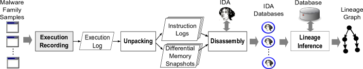
Figure 2: Approach overview. The execution recording and IDA tool are off-the-shelf components not developed in this work.

IV Approach Overview

Figure 2 summarizes our approach. It takes as input a set of program executables that belong to the same family and outputs a lineage graph. If the input malware samples are not labeled, as is often the case, we first cluster them using an off-the-shelf malware clustering approach (not shown in the figure). In this work, we use the AVClass tool [64], which clusters and labels samples into known families using the AV labels in VirusTotal [71] reports. While AV labels are known to be noisy [4, 50], AVClass successfully removes noise by performing label normalization, generic token detection, and alias detection. AVClass outputs for each sample the most likely family name and a confidence based on the agreement across AV engines.

Each family for which we want to analyze its lineage goes through processing depicted in Figure 2. For each sample in the family, our processing produces an output IDA database with the unpacked version of the sample’s code. The first step in the processing of each sample is to run it using an execution recording module, which performs a lightweight recording of the execution that can be deterministically replayed as many times as desired. For this, we use the off-the-shelf QEMU-based PANDA record and replay platform [54]. PANDA’s recording takes a snapshot of the VM state before execution and records non-deterministic changes to the CPU state and memory during execution. Such recording produces small changelogs and does not significantly slow down the VM (10%–20%), which limits time-related effects (e.g. network timeouts) on the target application. Using a record-and-replay platform enables separating the malware execution from the malware analysis. The small logs enable efficient storage of malware executions and the unpacking can be rerun every time an improvement is available.

The recording is used as input to the unpacking (Section V) and disassembly (Section VI) modules. The unpacking module replays the recorded execution, while monitoring the instructions executed and the memory writes they perform. Every time a memory area is written and then executed it identifies a wave and takes a snapshot of the memory of the program. For each wave, the unpacking module outputs 2 wave files: a differential memory snapshot that stores the content of the memory regions overwritten and an instruction log with the unique instructions executed in the wave. Programs with only one wave are not packed.

The disassembly module takes as input the wave files produced by the unpacking and outputs an IDA database with the unpacked code. It comprises of 3 steps: code region identification, function identification, and instruction disassembly. For each wave, it first loads the memory ranges in the differential memory snapshot into the IDA database, relocating them to a different address if that range is already occupied by previously unpacked content. Then, it applies function identification to find the start address of functions present in the differential memory snapshot. Finally, it informs IDA to disassemble inside each loaded range starting at the instruction addresses in the instruction log, and to create functions at the addresses identified by the function identification module.

The IDA databases for all samples in the family are input to the lineage inference module, which outputs the lineage graph (Section VII). The lineage inference module comprises of 3 phases. First, it computes the hashes of all functions in each IDA database and produces a program hash for each sample by hashing the concatenation of the function hashes. Second, it builds a lineage tree with the most likely parent for each node. Finally, it adds cross-edges to the lineage tree, by identifying if any node has additional parent nodes from which it inherits functions. This last step transforms the lineage tree into a lineage graph.

We have implemented our malware lineage approach using over 11K lines of C/C++ and scripts (Python and Bash), as measured by CLOC [13], i.e., without comments or blank lines. Of those, 5.8K lines correspond to the PANDA unpacking plugin, 1.5K to the IDA disassembly plugin, 3K to the lineage module, and 1K to scripts that glue the end-to-end processing.

V Unpacking

We desire four properties from our unpacking module: (1) Support for both off-the-shelf (e.g., Armadillo, PESpin) and custom packers. (2) Support for packers of different complexity (as defined by Ugarte et al. [68]). Specifically we want to support packers for which the unpacked original code may not be fully available in memory at any point of the execution, and samples that unpack code using multiple processes. However, we focus on packers that do not modify the original code, which excludes virtualization-based packers (e.g., Themida, VMProtect). (3) Maximize coverage, i.e., recover as much original code as possible. (4) Minimize noise, i.e., output as little code not part of the original code as possible.

We use the unpacking approach proposed by Bonfante et al. [8], which satisfies the first three properties mentioned above and to which we add differential memory snapshots to support the fourth property. Their approach runs the program and takes a memory snapshot before the first program instruction executes and at each wave change. Their wave semantics define when wave changes happen and guarantee that any code unpacked during execution will be present in a memory snapshot. Note that the unpacked code is a superset of the executed code, i.e., the memory snapshots typically contain much “dormant” original code, which was unpacked but not executed. For example, wave $W_{i}$ may unpack a function that contains a conditional. Only one branch of the conditional may be executed, but the code reachable through the other branch is also present in the memory snapshot taken before $W_{i+1}$ starts.

There are two main differences between [8] and our unpacking module. First, their unpacking code is not available and was built on top of Pin [46]. In contrast, our unpacking module is implemented as a plugin for the PANDA record and replay platform [54], which enables us to separate malware execution recording (which can be performed on dedicated malware farms [72, 40]) from the unpacking. It also provides better malware isolation and allows the future support of other QEMU-supported architectures. Second, our unpacking minimizes the noise by producing a differential memory snapshot for each wave, in contrast with the process-level snapshot produced by Bonfante et al. The motivation for this is that a wave’s snapshot shares much content with the snapshot of the prior wave. For example, the execution may first unpack a function $f_{1}$ and execute it (first wave), then unpack another function $f_{2}$ and execute it (second wave). In this case, the first snapshot contains $f_{1}$, while the second snapshot contains both $f_{1}$ and $f_{2}$. Removing the redundancy between snapshots reduces the noise in the IDA database output by the unpacking and disassembly modules.

Unpacking overview.

The unpacking module takes as input the execution log that records a run of a potentially packed program $P$. It replays the execution log and uses the wave semantics to identify waves in the list of tracked processes, which is initialized with the input process $P$ and to which any new process created (or injected from) a tracked process is added. At the beginning of the execution of each tracked process, a full memory snapshot of the process address space is taken. New waves are detected by monitoring, for each instruction executed by a tracked process, the memory ranges it may overwrite and whether previously overwritten bytes are being executed. For each new wave of a tracked process, the unpacking outputs a differential memory snapshot and a wave instruction log. The differential memory snapshot of wave $W_{i}$ stores the memory contents modified by the previous $W_{i-1}$ wave. It includes modified bytes in the main module, other modules, the heap, and the stack. The wave instruction log contains the instructions executed during the wave and marks instructions following calls as function entry points.

VI Disassembly

The unpacking module guarantees that the code the program unpacked during execution is present in the differential memory snapshots. However, it is present as part of a long sequence of raw bytes, which is not particularly useful. The goal of the disassembly module is given as input the instruction logs and differential memory snapshots produced by the unpacking, to output an IDA database where the instructions and functions in the unpacked code have been identified. IDA is arguably the most widely used reverse-engineering tool and already used by most malware analysts. Furthermore, popular IDA plugins exist for diffing two unpacked executables such as BinDiff [7] and Diaphora [16].

Next, we detail the three disassembly steps: memory range loading, function identification, and instruction disassembly.

Memory range loading.

The disassembly combines all the unpacked code into the same IDA database. This includes code unpacked by all the waves observed during execution, from the original process executed as well as from any child process it may create. Intuitively, if all the code comes from the same input packed executable, then it should be available together to the analyst as if the input executable was not packed. Loading the contents of the differential memory snapshots into the IDA database comprises of three substeps: removing duplicate ranges, (optionally) selecting ranges, and relocating overlapping ranges. The use of differential memory snapshots prevents a memory range unpacked in wave $W_{i}$ to appear in the snapshots of waves $W_{i+1},\dots,W_{n}$. But, some packers (e.g., YodaProtector) unpack the same content on the same memory range again and again. This behavior would introduce many duplicates of the same content in the IDA database. To prevent this, when a memory range is loaded into the IDA database, its original address and the hash of its contents are logged. If a range has the same original address and contents of another range already loaded, it is a duplicate and can be skipped.

By default, all (non-duplicate) memory ranges in the differential memory snapshots are loaded into the IDA database. This includes ranges in the regions of the main module, other modules, heap, and stack. Some of those ranges may only contain data. An analyst, depending on the end application, may prefer to exclude data ranges to reduce the size of the final IDA database. The disassembly module allows an analyst to specify filters on which ranges should be loaded. For example, an analyst could specify that ranges on the stack or the heap should not be loaded, or that only ranges in pages with execution permission should be loaded.

While loading the selected memory ranges, the disassembly module monitors if two memory ranges overlap. If so, one of them needs to be relocated because IDA does not support having multiple contents at the same memory range. Internally, IDA uses a linear address space where analysts can create segments, which represent contiguous chunks in the linear address space. Creating a segment requires the start and end addresses of the segment in the linear address space, and the segment base. The segment base is used to compute virtual addresses for the segments, which are the addresses an analyst sees. The conversion from linear to virtual addresses is: $VirtualAddress=LinearAddress-(SegmentBase<<4)$. The disassembly module loads each range in each wave of each tracked process as a separate segment. It starts by creating a segment at the base address of the main module of the initial malware process, which corresponds to the contents of the packed malware sample. For each wave of the initial malware process, it creates another segment following the previous one in the linear address space, adjusting the segment base so that virtual addresses in the new segment follow virtual addresses in the prior segment. When a wave is relocated, the disassembly module scans the disassembled instructions and rewrites any addresses found in the disassembled code to point to the same location as before the relocation. Once all waves of the initial process have been loaded, the memory range loading repeats for any other tracked processes.

Function identification.

An important step when disassembling a program is identifying functions. Our disassembly module uses two techniques to locate function entry points and instructs IDA to create functions at those addresses. First, it uses the instructions marked in the wave instruction log to have followed a call instruction. This helps identify targets of indirect calls that appeared in the execution. Second, it uses ByteWeight [5] to locate the start address of functions in each of the regions loaded into the IDA database. This method can identify the entry point of functions that did not execute during unpacking. However, ByteWeight identifies functions in the text section of an input executable. Instead, we want to identify functions in the raw regions of memory contained in the differential memory snapshots. Thus, we have modified ByteWeight to take as input a sequence of assembly instructions, rather than a full executable. Our disassembly module first disassembles 10 instructions starting at each offset in a region and inputs those instructions to the modified ByteWeight, which outputs a score between 0 and 1 indicating how likely the disassembled instructions correspond to a function start. As recommended in [5], the address of any sequence of instructions with a score higher than 0.5 is considered a function start.

Instruction disassembly.

The instruction disassembly leverages the function start addresses identified by ByteWeight and dynamic information from the execution, e.g., to identify targets of executed indirect jumps. First, our disassembly module instructs IDA to start disassembling at every identified function start address. Then, it instructs IDA to start disassembling at every instruction in the wave instruction logs. For this, the information in the instruction log is used to identify which wave unpacked the instruction, which is used to locate the IDA segment where the instruction has been loaded. Note that when IDA is instructed to disassemble at an address, it performs a recursive disassembly to find as much code as possible. Thus, it also disassembles dormant code captured in the differential memory snapshots, which did not execute during the execution recording.

VII Lineage Inference

The lineage inference module takes as input the IDA databases of the family samples with the unpacked and disassembled code and produces the lineage graph. It comprises of three phases. The first phase identifies the nodes in the lineage graph (Section VII-A) and also constructs the $L$ and $F$ functions (see Section II). The other two phases identify the edges in the lineage graph. The second phase builds a lineage tree starting with a selected root and greedily inserting the most similar node, not yet in the tree, to any node already in the tree (Section VII-B). In the lineage tree each node has at most one parent. The third phase identifies whether some nodes inherit code from multiple nodes and thus need to have more than one parent (Section VII-C). The complexity analysis of the three phases is provided in Appendix -A.

VII-A Phase I: Identifying Versions

Identifying the set of nodes in the lineage graph requires finding which input samples correspond to each family version. In our approach, two input samples are the same version if they have the same set of functions. To uniquely identify a function we use a function hash. The use of a function hash is critical for scalability. It enables identifying all samples that contain a specific function in $O(1)$, a fundamental step in phase III.

Our approach works with different function hashes. Each hash can have different properties and may produce a different set of nodes for the lineage graph. Overall, we seek function hashes that determine that two functions are the same with low false positives, and are efficient to compute and index. Currently, our approach supports two such function hashes:

Raw hash.

Performs an MD5 hash of the sequence of raw byte values from function start to function end. Two functions with the same raw hash have the same bytes and thus are the same function. This hash does not require disassembly and should not produce false positives. On the other hand, it can have high false negatives when modifications have been applied to the function that do not affect its functionality, e.g., semantics-preserving instruction reordering. We use this hash as baseline for comparison.

SPP-NOP hash.

The small prime product (SPP) assigns to each instruction mnemonic a small prime number. The hash corresponds to the product of the primes of all mnemonics of the instructions in the disassembled function [18]. We have modified the SPP hash computation to ignore instructions used for padding that do not affect the function semantics, e.g., the no-op (NOP) instruction and a move from a register to the same register. The advantage of SPP-NOP over the raw hash is that it can detect the same function despite instruction reordering, block reordering, and instruction padding.

This phase first iterates on all the functions in each input IDA database, computing both the raw and SPP-NOP function hashes, and storing them in a central database. Short functions with at most two instructions are ignored. Then, it computes a raw program hash and a SPP-NOP program hash for each sample by sorting the (raw or SPP-NOP) function hashes for the sample, concatenating them separated by a delimiter, and hashing the concatenation using MD5. Each program hash represents one version in the lineage graph. Samples with the same program hash are polymorphic variants of the same version.

The raw and SPP-NOP hashes may produce different sets of nodes for the lineage graph. The raw hash gives an upper bound on the number of nodes since it should not have false positives. Thus, the number of nodes using the SPP-NOP hash is always less than or equal to the number of nodes using the raw hash. While they can produce different node sets, both hashes often agree. Specifically, in 10 out of 13 open-source programs and in 1 out of 10 malware families evaluated, both hashes produce the same set of nodes.

Input: Family versions $V=\{v_{1},v_{2},\dots,v_{n}\}$

Output: Lineage tree T

1 begin

2       T $\leftarrow(\{\},\{\})$

3       // Pick smallest node as root

4       v $\leftarrow$ minNode(V)

5       T.addNode(v)

6       V.remove(v)

7      

8      // Greedily insert nodes

9       while $V\not=\{\}$ do

10             // $p\in T.V,v\in V$

11             (p,v) $\leftarrow$ findMostSimilarPair(T,V)

12             T.addEge(p,v)

13             V.remove(v)

14            

15       end while

16      return(T)

17      

18 end

19

Algorithm 1 Lineage graph inference phase II.

VII-B Phase II: Building a Lineage Tree

Given the nodes identified in Phase I, Phase II greedily builds a lineage tree where each node has a single parent. Its processing is described in Algorithm 1. Starting with an empty tree, it first inserts as root the node that minimizes the sum of its size (i.e., number of functions) and the average distance to all other nodes. This root selection is inspired by Lehman’s 6 software evolution law (“Continuing growth”), which states that programs tend to grow over time [42]. Then, it iterates inserting at each step the node, not yet in the tree, with the highest number of shared functions to any node already in the tree. The iteration terminates when all nodes have been inserted.

The function findMostSimilarPair greedily selects the next edge to insert and needs to handle two classes of ties. First, there could be multiple candidate nodes not yet in the tree that share the same number of functions with a node already in the tree. Here, the candidate with highest number of instructions shared with a node in the tree is selected. Second, the node to be inserted could share the same number of functions (or instructions) with multiple nodes already in the tree. Among those, the node latest inserted in the tree is picked as parent.

An special case happens when the remaining nodes, not yet in the tree, share very few (or no) functions with nodes already in the tree (we use an experimentally determined threshold of less than 2% similarity). This may indicate independent development lines or a large refactoring of the code. In this case, the algorithm picks the smallest node not yet in the tree as the next to insert, rather than the one most similar to a node in the tree (since none remaining are similar to those in the tree). An edge is added between the selected node and the most similar node in the tree. If the number of shared functions is zero, phase III will later remove those edges, thus introducing multiple independent lines.

Input: Lineage tree T

Output: Lineage graph $G$

1

2begin

3       G $\leftarrow$ T.removeZeroSimilarityEdges()

4       V $\leftarrow$ topologicalSort(G.V)

5       foreach $v\in V$ do

6             // Find added functions (not in parent)

7             p $\leftarrow$ G.findParent(v)

8             $F_{a}\leftarrow$ F(v) $\setminus$ F(p)

9             // Find candidate parents for cross-edge

10             C = G.V $\setminus$ (G.successors(v) $\cup$ G.predecessors(v))

11             // Find cross-edges

12             X = findCrossEdges($F_{a}$,C)

13             // Add cross-edges to graph

14             foreach $(p,c)\in X$ do

15                   G.addEdge(p,c)

16                  

17             end foreach

18            

19       end foreach

20      return(G)

21      

22 end

23

Algorithm 2 Lineage graph inference phase III.

VII-C Phase III: Adding Cross-Edges

Each node in the lineage tree has at most one parent. However, it is possible for a version to descend from multiple versions, e.g., when a development branch is merged back into the trunk. Phase III identifies versions with multiple parents.

Algorithm 2 describes this phase. The first step is to remove any edges with zero shared functions. This removal introduces additional roots, identifying independent development lines. Then, it iterates on the nodes in topological order. For the current node, it first computes the set of added functions, i.e., functions in this version that are not inherited from the parent version. Then, it selects the candidate parents for a cross-edge, which are the nodes that are not successors or predecessors of the current node. Successors are ignored because a cross-edge from them would introduce a cycle in the graph. Predecessors are ignored because they already influence the current node. Function findCrossEdges picks among the parent candidates the one that shares the most added functions with the current node. Then it removes those functions from the set of added functions and picks the next node that shares the most remaining added functions. The process terminates when no candidates share more than a threshold $t$ of functions, which we have determined experimentally to be 3. Once findCrossEdges returns, the cross-edges are added to the graph. Note that the use of a function hash is fundamental in findCrossEdges because it allows us to query in $O(1)$ time if a function in the set of added functions is present in any candidate parent.

VIII Evaluation on Benign Programs

In this section we evaluate the accuracy of our approach on benign open-source programs for which we have ground truth. Section VIII-A presents the accuracy metrics, Section VIII-B the unpacking and disassembly results, and Section VIII-C the lineage inference results. The evaluation on malware is in Section IX.

Packer	Version	$|P|$	FC			FNR
			Min	Avg	Max	Min	Avg	Max
ACProtect	2.0	21	48.68%	68.73%	79.79%	23.74%	39.57%	76.00%
Armadillo	8.20	2	61.22%	61.74%	62.26%	32.65%	35.71%	38.78%
ASPack	2.12	21	46.91%	70.48%	81.53%	16.62%	24.18%	40.35%
eXPressor	1.8.0.1	21	47.01%	70.58%	81.53%	16.74%	24.79%	43.33%
FSG	2.0	21	46.91%	70.48%	81.53%	15.69%	21.49%	30.73%
MEW 11 SE	1.2	21	46.91%	70.48%	81.53%	16.47%	22.60%	31.14%
MoleBox	2.5.13	21	48.78%	68.63%	79.79%	27.87%	46.28%	86.55%
MPRESS	2.19	21	49.14%	69.46%	80.14%	15.23%	22.24%	33.33%
Packman	1.0	21	46.91%	70.48%	81.53%	15.84%	21.77%	30.87%
PECompact	1.71	21	46.91%	70.48%	81.53%	16.08%	22.58%	33.33%
PELock	2.04	21	48.78%	69.25%	79.79%	25.81%	36.61%	47.73%
PESpin	1.33	21	48.68%	67.49%	79.44%	20.26%	29.25%	55.74%
Petite	2.4	21	47.01%	70.48%	81.53%	15.97%	22.28%	32.00%
RLPack	1.21	21	48.62%	69.10%	79.79%	17.02%	24.55%	39.29%
UPX	3.91	21	47.01%	70.48%	81.53%	15.66%	21.16%	30.73%
WinUPack	0.39	21	46.91%	70.48%	81.53%	15.69%	21.39%	30.73%
YodaCrypter	1.3	20	48.68%	69.14%	79.79%	16.79%	24.31%	41.18%
YodaProtector	1.03	21	48.68%	68.74%	79.79%	22.37%	34.69%	71.96%
All		21	46.91%	69.26%	81.53%	15.23%	27.53%	86.55%

TABLE I: Unpacking and disassembly accuracy evaluation on all SPEC CPU 2006 C programs with SPP-NOP, each packed with 18 packers. For each packer it shows the number of programs evaluated, function coverage, and function noise ratio.

VIII-A Accuracy Metrics

No prior unpacking approach proposes metrics to scientifically quantify the quality of the unpacking. Quoting a recent unpacking work: “we recognize that we have not been able to define a metric that allow us to adequately determine code coverage” [8]. We propose to evaluate the accuracy of the unpacking and disassembly process by measuring how similar the original program (before packing) is to its unpacked representation. For this, we compare the IDA database of the original program, disassembled using symbol information to prevent errors, with the IDA database output after packing the program, and processing the packed program with the unpacking and disassembly modules.

We propose two new metrics that separately quantify the amount of original code recovered and the amount of noise. We denote the set of functions in the original program database $F_{o}$ and in the unpacked program database $F_{u}$. We denote the set of correctly unpacked original functions as $F^{o}_{u}\subseteq F_{u}$. Correctly unpacked functions are the unpacked functions also present in the original code, i.e., $F^{o}_{u}=F_{u}\cap F_{o}$. Intuitively, unpacked functions that are not original code can be considered noise, i.e., $F^{n}_{u}=F_{u}\setminus F^{o}_{u}$. This noise includes, among others, unpacking functions and falsely identified functions during disassembly. Given the original and noise functions in the unpacked output, we define two metrics to evaluate accuracy: function coverage (FC) and function noise ratio (FNR).

Function coverage.

The fraction of original functions the unpacking recovers over the number of functions in the original program. Ranges from zero (no original functions recovered) to one (all original functions recovered):

$$FC=\frac{|F^{o}_{u}|}{|F_{o}|}=\frac{|F_{u}\cap F_{o}|}{|F_{o}|}$$ (1)

Function noise ratio.

The fraction of noise functions over the total number of functions in the unpacked representation of the program. Ranges from zero (no noise) to one (all noise, no original functions recovered):

$$FNR=\frac{|F^{n}_{u}|}{|F_{u}|}=\frac{|F_{u}\setminus F^{o}_{u}|}{|F_{u}|}$$ (2)

When computing FC and FNR we identify a function by its SPP-NOP hash, and we ignore short functions, i.e., those with at most two instructions, since those can cause spurious matches.

VIII-B Unpacking & Disassembly Accuracy

We evaluate the accuracy of the unpacking and disassembly modules using a dataset of 21 programs for which we have the source code: 19 C programs from the SPEC CPU 2006 benchmark [67] and 2 C++ programs from the Olden benchmark [45]. We compile them using Visual Studio with optimization level -O2 and debugging symbols, producing an executable and a PDB symbols file. We use IDA to disassemble them providing the PDB symbols file as input. Next, we pack the executables with 18 off-the-shelf packers and examine that they work. We find that the SPEC CPU 2006 programs do not work after packing with Armadillo, but the 2 Olden benchmark programs work. There is also one SPEC CPU 2006 program that does not work after being packed with YodaCrypter. We input the correctly packed executables to the unpacking and disassembly modules, which output an IDA database with the recovered code.

Table I summarizes the accuracy results using the metrics described in Section VIII-A. Overall, our unpacking and disassembly modules achieve an average function coverage of 69% and an average function noise ratio of 27%. Manual analysis of the results shows that: (a) all original functions are present in the differential memory snapshots and thus in the unpacked IDA database, (b) the same functions are missed in a program regardless of the packer, (c) the disassembly process fails to identify always the start of the same functions, and (d) the vast majority of additional functions (i.e., noise) are added by the packing process to perform the unpacking at runtime. Thus, all the original code is present in the differential memory snapshots output by the unpacking, but, regardless of the packer, the disassembly process fails to identify the entry point of the same functions. Next, we analyze this issue in more detail using the BHBmk program from the Olden benchmark. We observe the same causes in other programs.

For BHBmk, the analysis reveals that ByteWeight only finds 37 original functions (i.e., misses 15 functions) despite all functions being present in the differential memory snapshots provided as input to ByteWeight. Manual analysis on the missed functions shows two reasons. First, 9 functions are wrappers to other functions. These wrappers start with a sequence of push instructions followed by a call to the wrapped function, which is a common sequence in the middle of functions and thus not detected by ByteWeight as a function entry point. Second, 6 functions have uncommon preambles not in the ByteWeight model. Note that even if ByteWeight misses a function start, IDA may still identify the function if there is a direct call to it. Of the 15 BHBmk functions missed by ByteWeight, IDA identifies 10 this way. There are also 4 functions whose start address ByteWeight finds, but IDA refuses to create a function at that address. There are two reasons for this. First, IDA may run into a disassembly error inside the function failing to find the function’s boundary. Second, IDA may have already marked that code as belonging to another function and refuses to create a new function there.

To conclude, the unpacking module properly outputs all original code into the differential memory snapshots, but not all original functions would be available to the lineage inference because the disassembly misses some functions. Most of the missed functions are due to ByteWeight and we plan to either improve it or replace it in our next release. Most of the additional functions (i.e., noise) implement the unpacking process and we plan to identify those as a next step.

			Reference			SPP-NOP				Raw				iLine (PO)		BinDiff
Program	First	Last	Type	Rel.	$|V|$	$|V|$	$|R|$	$|X|$	PO	$|V|$	$|R|$	$|X|$	PO	DAG	SL	$|V|$
FileZilla	3.0.0	3.24.0	S	121	119	119	1	18	99%	121	1	20	97%	96%	100%	118
Fzputtygen	3.0.8	3.24.0	S	108	19	19	1	0	100%	30	1	0	96%	51%	99%	18
Fzsftp	3.0.0	3.24.0	S	118	50	50	1	0	91%	52	1	2	34%	38%	48%	43
Notepad++	1.0	7.3	D	70	70	70	1	6	64%	70	1	14	71%	76%	71%	70
Pageant	0.50	0.67	S	18	18	18	1	0	93%	18	1	0	97%	84%	99%	18
Plink	0.50	0.67	S	18	18	18	1	0	98%	18	1	1	90%	84%	99%	17
ProcessHacker	1.0	2.39	2-S	52	52	52	2	1	99%	52	2	8	79%	86%	100%	52
PSCP	0.48	0.67	S	20	20	20	1	1	99%	20	1	1	73%	96%	99%	19
PSFTP	0.52	0.67	S	16	16	16	1	0	99%	16	1	0	88%	95%	99%	15
PuTTY	0.46	0.67	S	22	22	22	1	2	100%	22	1	0	92%	98%	99%	21
PuTTYgen	0.51	0.67	S	17	16	16	1	0	99%	16	1	0	75%	87%	99%	16
PuTTYtel	0.49	0.52	S	4	4	4	1	1	100%	4	1	0	50%	100%	100%	4
WinSCP	4.2.6	5.9.3	S	47	47	47	1	1	99%	47	1	8	94%	99%	100%	47

TABLE II: Lineage inference evaluation on 13 open-source programs. For each program, it first shows the earliest and last versions analyzed. Then, the expected lineage graph type (S for straight-line, 2-S for two straight lines, and D for DAG), the number of releases, and the number of expected binary versions (i.e., ground truth). Next, for the lineage graph generated using each hash: the number of nodes ($|V|$) and root nodes ($|R|$), the number of cross-edges ($|X|$), and the partial order (PO) agreement. The next two columns show the PO agreement using iLine’s DAG and straight-line (SL) algorithms. The final column shows the number of versions identified using BinDiff.

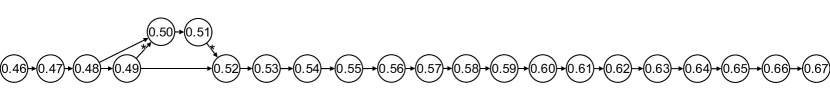
Figure 3: PuTTY lineage graph. Cross-edges are marked with asterisk.

Figure 4: Fzputtygen lineage graph.

VIII-C Lineage Inference Accuracy

To evaluate the lineage inference we use 631 release versions of 13 open-source Windows programs. Seven of the programs are part of the PuTTY distribution [59] (PuTTY, PuTTYgen, PuTTYtel, PSFTP, PSCP, Plink, Pageant), three are part of FileZilla [21] (FileZilla, Fzputtygen, Fzsftp), and the other three are WinSCP [75], Notepad++ [52], and ProcessHacker [58]. We are interested in evaluating the lineage inference as a stand-alone module. Thus, we evaluate on the released (i.e., unpacked) executables. To evaluate a program, we generate an IDA database for the executable of each version and input these IDA databases to the lineage inference module to produce the lineage graph. Then, we compare the lineage graph to the expected lineage graph built using the version numbers.

We manually identify the number of binary versions among the input releases. There are three main reasons why consecutive source releases may not create a new binary version. First, some versions do not modify the source code, but only auxiliary files (e.g., configuration files, images). This happens, for example, between FileZilla 3.9.0 and 3.9.0.1. Second, some versions perform source code modifications that do not affect the final executable, e.g., variable renaming. Third, in distributions with multiple programs, source code changes may affect some programs, but not others. For example, the changes between 0.61 and 0.62 affected PuTTY and PuTTYtel, but not PuTTYgen. Thus, PuTTYgen 0.61 and 0.62 are the same binary version.

Table II summarizes the results. For each program it shows the first and last versions analyzed. Then, it shows the expected lineage graph type, the number of releases, and the number of binary versions (i.e., ground truth). The type can be S for straight-line, 2-S for two straight lines, and D for branching and merging, i.e., DAG. Next, it shows for the lineage graph generated using each hash: the number of nodes and root nodes, the number of cross-edges, and the partial order agreement, a measure of lineage graph accuracy proposed in iLine [33]. Finally, it shows the PO agreement using iLine’s DAG and straight-line algorithms.

The results for Phase I show that the versions identified by the SPP-NOP hash match the expected binary versions for all 13 programs, while the raw hash identifies the correct binary versions for 9 programs. For the 3 FileZilla programs, the number of nodes identified by the SPP-NOP and raw hashes differs, with the raw hash identifying a larger number of binary versions. In all cases, when a node in the lineage graph represents multiple releases (each with a different executable hash), those releases are consecutive. These results indicate that the SPP-NOP hash is better at identifying versions than the raw hash.

Analysis of the phase II results shows that the generated lineage tree is more accurate with the SPP-NOP hash in 9 programs and has the same accuracy with both hashes in 4 programs. Thus, the SPP-NOP hash works better than the raw hash also in this phase. The most common error is that a version $x$ is more similar to version $x+2$ than to version $x+1$. These errors happen in all but one program and manifest in two cases: two consecutive versions swap their positions or a version has two successors one creating a branch with a single node and no merging point. An example of the first case is PuTTYgen where version 0.58 is followed by 0.60, which is followed by 0.59. An example of the second case is Fzsftp version 3.0.6, which is followed by both 3.0.7.1 and 3.0.8.1. The latter is followed by all other versions, while 3.0.7.1 is in a branch by itself. Another error affecting 2 programs is that the wrong root is chosen, i.e., the chosen root is not the earliest version, but the second earliest.

All programs have the correct number of roots, one for straight line or DAG development, and two for ProcessHacker that has two separate lines. For the 12 programs with straight-line (or 2-straight) development, phase III can only introduce errors as there is no branching and merging. But, our algorithm should identify those cases and avoid inserting cross-edges. The results show that cross-edges are inserted for 7 programs. In 5 of those programs only 1 or 2 cross-edges are inserted and these typically are inserted where there was an error in Phase II. For example, Figure 3 shows the final lineage graph for PuTTY. Version 0.48 is followed by versions 0.49 and 0.50 after Phase II, and phase III inserts cross-edges between 0.49 and 0.50 and between 0.51 and 0.52. If 0.50 had followed 0.49 after Phase II, no cross-edge would have been inserted as 0.49 would be a predecessor of 0.50 and thus not included in the list of candidate parents. The same applies to the cross-edge from 0.51 to 0.52. Figure 4 shows the final lineage graph for Fzputtygen. In this case, the lineage graph has no errors and perfectly matches its straight-line development.

Comparison with iLine.

We compare our lineage inference algorithm with iLine, the current state-of-the-art lineage inference approach. iLine proposes two different lineage inference algorithms for straight-line code and branching and merging, and assumes the analyst knows which of the algorithms should be used (or which results to trust if both algorithms are used). Since iLine is not publicly available we have re-implemented both of its algorithms. The two rightmost columns in Table II show the results for iLine’s DAG and straight-line (SL) algorithms using as symmetric distance the number of differing functions between both samples according to the SPP-NOP hash. This allows us to compare iLine’s algorithms with our algorithm using similar features. To measure accuracy, we use the partial ordering agreement (PO) metric proposed in iLine. For ProcessHacker, we first split versions into both development lines and apply iLine’s SL algorithm in each line separately. Our lineage inference module using SPP-NOP achieves an average 95% PO over the 13 programs, compared to 84% for iLine’s DAG and 93% for iLine’s straight line. Thus, our algorithm outperforms both of iLine’s algorithms despite using no apriori knowledge about the development model, which is fundamental when operating with malware. The best results for iLine are obtained by assuming straight-line development, but this means that a wrong (straight-line) lineage graph would be produced for any program using branching and merging.

Comparison with BinDiff.

We compare our Phase I results with BinDiff. Pairwise comparison of all versions does not finish in 8 hours for WinSCP and FileZilla. To address this, we first partition the executables by number of functions (i.e., executables with differing number of functions should be different versions) and only perform pairwise comparisons inside each partition. After aligning two executables with BinDiff we consider they are the same version if BinDiff successfully aligns all the functions in both executables and the similarity value for each function is over 0.9. The righmost column in Table II shows that in 7 out of 13 programs, this approach would introduce errors, i.e., incorrectly identifying similar versions as being the same. Furthermore, note that we cannot use BinDiff in Phase III of our algorithm because it cannot check if a function appears in any of the predecessor nodes. We need function hashes for that.

Figure 5: Lineage graph for PuTTY when each version is packed with a different packer.

Packed evaluation.

To evaluate the lineage inference accuracy with packed executables, we perform the following experiment. We pack each version of PuTTY using a randomly selected packer and then apply the unpacking, disassembly, and lineage inference modules to build the lineage graph. This allows us to evaluate our lineage inference approach when different packers are used by the same program, as well as to check the impact on the lineage graph of any functions missed by the unpacking and disassembly modules. Figure 5 shows the produced lineage graph, which is identical to the unpacked version in Figure 3.

In summary, our evaluation has shown that: the SPP-NOP hash outperforms the raw hash both in node and edge identification; the lineage graphs produced using the SPP-NOP hash are more accurate than those produced by iLine, without assuming a specific development model was used; our version identification improves on BinDiff; and the lineage graphs are accurate despite the use of different packers.

		Unpacking										Disassembly
Family	EXE	Instructions (M)			Processes			Waves			Time	$|F_{u}|$			Time
		Min	Avg	Max	Min	Avg	Max	Min	Avg	Max	Avg(s)	Min	Avg	Max	Avg(s)
Allaple	4,000	0.006	3.1	497.7	1	1.00	1	1	4.00	5	399	11	25	458	59
IRCbot	365	0.1	54.5	655.9	1	1.99	3	1	3.87	5	460	5	655	700	114
Klez	750	6.8	7.8	11.6	1	1.00	1	1	4.93	5	126	5	749	810	65
Loring	216	36.2	49.6	51.9	2	2.00	2	2	3.99	4	361	84	697	700	164
Memery	113	172.2	282.6	298.5	1	1.00	1	2	2.00	2	1,483	127	127	128	27
Picsys	131	7.8	11.0	11.3	1	1.00	1	1	1.96	2	513	24	698	737	109
Simbot	214	29.7	101.0	202.1	1	2.00	3	2	4.29	5	671	18	85	160	56
Sytro	1,354	2.6	4.5	8.2	1	1.00	1	1	1.87	2	119	21	702	810	33
Urelas	206	0.006	252.8	924.1	1	3.61	7	1	9.29	215	860	57	2,171	5,951	366
VtFlooder	444	0.006	1,379.5	3,439.3	1	1.00	1	1	2.26	6	1,927	10	138	1,058	36

TABLE III: Unpacking and disassembly results on packed malware. For each family, it shows the executables analyzed, instructions (in millions) traced for all malware processes, malware processes traced; waves for all malware processes, unpacking runtime, number of unpacked functions in the IDA databases, and disassembly runtime.

IX Evaluation on Malware

This section evaluates our lineage approach on 10 malware families. We first describe our dataset, then in Section IX-A we present the unpacking and disassembly results, and in Section IX-B the lineage inference results.

Dataset.

The PANDA team periodically records malware executions on a sandbox and makes these recordings publicly available [55]. The malware in those recordings is unlabeled, i.e., its family is unknown. To classify the malware, we first collect the AV labels for the samples using VirusTotal (VT) [71], an online service that analyzes files and URLs submitted by users. We use the AV labels as input to AVClass [3], an open-source malware labeling tool. AVClass outputs for each sample the most likely family name and a confidence factor based on the agreement across AV engines [64]. To compute the lineage graph we need a significant number of samples for the same family. Thus, we select 10 malware families for which more than 100 samples are labeled with high confidence by AVClass: Allaple, IRCbot, Klez, Loring, Memery, Picsys, Simbot, Sytro, Urelas, and VtFlooder. In total we evaluate on 7,793 malware samples. The largest number of family samples is 4,000 for Allaple and the smallest 113 for Memery.

IX-A Unpacking and Disassembly

Table III details the unpacking and disassembly results for the 10 malware families. For each family, it shows: the number of executables analyzed; the number of instructions (in millions) traced for all malware processes; the number of malware processes traced; the number of waves for all malware processes; the unpacking runtime (in seconds); the total number of unpacked functions in the IDA databases (including short and external functions that IDA counts); and the disassembly runtime (in seconds).

For 6 families all samples have a single process, for Loring all samples have 2 processes, and the remaining three (i.e., IRCbot, Simbot, Urelas) have samples with different number of processes. The number of waves ranges from 1 (i.e., not packed) up to 215 for a Urelas sample. Surprisingly, 7 families have a few samples that are not packed (e.g., 5 out of 131 samples in Picsys), which may be due to the developers forgetting to pack some samples or to early versions not being packed. On average, replaying a recording takes 11 minutes, the slowest being VtFlooder with an average of 32 minutes per recording. The disassembly runtime takes on average 103 seconds per sample, of which 82% is due to the ByteWeight function identification.

		$|V|$		$|E|$		$max(|L(v_{i})|)$		$|L(v_{i})=1|$		$max(|F(v_{i})|)$		$min(|F(v_{i})|)$		$|\bigcup F(v_{i})|$
Family	EXE	spp	raw	spp	raw	spp	raw	spp	raw	spp	raw	spp	raw	spp	raw
Allaple	4,000	6	311	5	310	2,742	2,742	0	278	12	301	11	10	2,387	5,847
IRCbot	365	11	12	4	5	338	338	8	9	510	545	2	2	700	980
Klez	750	64	66	63	68	585	585	47	49	619	667	5	5	691	1,114
Loring	216	2	3	1	2	215	127	1	1	510	545	60	61	521	726
Memery	113	9	9	8	8	65	65	3	3	121	123	120	122	130	134
Picsys	131	3	4	2	3	95	95	0	1	379	473	16	16	387	736
Simbot	214	37	110	36	109	65	48	23	94	67	72	17	17	126	1,989
Sytro	1,354	6	7	5	4	811	811	0	0	618	667	13	13	758	1,509
Urelas	206	123	130	213	179	22	22	105	115	3,702	4,420	42	44	7,725	78,408
VtFlooder	444	32	95	39	95	228	228	16	82	905	945	10	10	5,324	9,397

TABLE IV: Lineage graph details. For each hash, it details the number of versions, edges, the maximum number of samples in a version, the number of singleton versions representing a single sample, the maximum and minimum number of functions in a version, and the total number of functions across all versions.

Figure 6: Lineage graph for Sytro built using 1,354 samples. The node label indicates the number of functions in the version and the number of samples of that version. The edge label is the number of shared functions.

IX-B Lineage Inference

Table IV details the final lineage graphs output for the 10 malware families. The table shows the number of executables for each family and for each hash: the number of nodes and edges, the maximum number of samples in a version, the number of singleton versions representing only one sample, the maximum and minimum number of functions in a version, and the total number of functions across all versions.

We focus on the SPP-NOP hash results as Section VIII-C demonstrates that it outperforms the raw hash. The largest number of SPP-NOP versions is for Urelas with 123 and the smallest for Loring with 2. For 9 families, the number of versions using both hashes differs. Overall, we identify 293 SPP-NOP versions across the 10 families, compared to 7,793 input samples, a 26 times reduction (10x reduction for the raw hash). Thus, our lineage graph is a succinct summary of family evolution, achieving over an order of magnitude reduction in nodes compared to prior approaches where each input sample is a node.

The results show that some versions are more popular than others in terms of samples. For example, 99% of Loring and 92% of IRCbot samples are derived from one version. On the other hand, 51% of Urelas samples correspond to singleton versions, which may be due to a large amount of experimentation in the family, or to limited coverage of our input samples for some versions. The code of a family can significantly evolve over time. For example Urelas versions range from 42 up to 4,420 functions. We also observe different code base sizes across families. The most complicated malware families are Urelas and VtFlooder with 7.7K and 5.3K functions across all versions, respectively. The simplest malware family is Simbot with a total of 126 functions in 216 samples.

Of the 10 malware families, 3 have straight-line development (Allaple, Loring, Picsys). Figure 1 shows the final Picsys lineage graph. Memery and Sytro have mostly straight development with only one node having two branches, one of them leading to a single node, as illustrated in the lineage graph for Sytro in Figure 6. Simbot has mostly straight development with 4 nodes having two branches. IRCbot has multiple straight lines, although 98% of the input samples belong to the same line. Finally, the lineage graphs of 3 families (Klez, Urelas, VtFlooder) are DAGs. These results show the variety of development models malware families may use and the difficulty of predicting the development model apriori.

To conclude the results show that the lineage graph is a succinct summary of the evolution of a malware family, which reduces the number of input samples to a much smaller (i.e., 26 times smaller) number of versions. The 10 malware families show varying development models that are captured by our lineage inference algorithm.

X Discussion

This section discusses some limitations of our work and directions for future investigation.

Packers that modify the original code.

Our unpacking module handles packers where the original code is recovered at runtime. However, packers may transform the original code, so that it is no longer present in the packed executable. For example, virtualization-based packers such as Themida and VMProtect convert assembly into bytecode interpreted by a VM. One approach to handle such packers is analyzing the executable code output by the interpreter. We leave the support of such packers as future work.

Evasion.

Similar to other dynamic analysis approaches, our unpacking can be evaded by techniques that detect the presence of a VM or emulator. We ameliorate this problem by incorporating countermeasures for specific anti-VM checks, but our countermeasures are not complete. Interestingly, we observe that anti-VM checks are typically packed themselves to avoid their presence flagging the executable as malware. If the anti-VM checks are unpacked simultaneously with the original code, by the time the malware executes the anti-VM checks our unpacking has already captured the original code in a differential memory snapshot.

Code semantics.

Our approach enables comparing the functions added and removed across versions of a malware family. However, the analyst still needs to examine the added and removed functions to understand their functionality. In future work, we plan to provide the analyst with summaries of the semantics of those functions to further reduce the malware analysis effort.

Function identification.

Most disassembly errors in our evaluation are due to missed functions. Our system currently uses ByteWeight [5] for function identification, but could use other tools. We are currently evaluating Nucleus [2], which should improve on ByteWeight results, but have not finished integrating it into our toolchain yet.

XI Conclusion

We have presented a novel malware lineage approach that works on malware collected in the wild. Given a pool of malware executables from the same family, it produces a lineage graph where nodes are family versions and edges describe their descendant relationships. We have proposed the first technique to identify different versions of a malware family and a scalable code indexing technique for efficiently identifying functions shared between any pair of versions. We have evaluated the accuracy of our approach on 13 benign programs and produced lineage graphs for 10 malware families, showing that the produced lineage graphs are a succinct representation of the evolution of a malware family.

-A Complexity Analysis

Let the set of malware samples be $S=\{s_{1},\cdots,s_{n}\}$ and $\mathcal{F}$ be the set of functions appearing in all malware samples in $S$. Let $F:S\rightarrow 2^{\mathcal{F}}$ label each malware with the set of functions appearing in it (e.g., $F(s_{2})=\{f_{5},f_{8}\}$ means that functions $f_{5}$ and $f_{8}$ appear in $s_{2}$). Our algorithm is divided into three phases.

Phase I (clustering): The goal of this phase is to find a coarsest partition $\mathcal{P}\;=\;\{G_{1},G_{2},\cdots,G_{k}\}$ of $S$ such that $s_{i}$ and $s_{j}$ are in the same group iff $F(s_{i})=F(s_{j})$. Using hashing, the cost of finding this partition is $O(n)$. We overload the function $F$, and use $F(G_{i})$ to be $F(s)$ for some $s\in G_{i}$ (since all $s\in G(s_{i})$ have the same label $F(s)$, picking an arbitrary $s$ does not create an issue.)

Phase II (Lineage Tree): This tree $T=(V,E)$ has $k$ vertices $\{1,\cdots,k\}$, where vertex $i$ corresponds to group $G_{i}$. Let $\mbox{inst}(s_{i},s_{j})$ be the number of instructions common between $s_{i}$ and $s_{j}$. We say that $G_{i}\prec G_{j}$ iff $F(i)\subset F(j)$. For each $j\in V$, define $\mbox{dist}(i,j)$ (for $i\in V$) to be the $2$-tuple $\langle|F(G_{i})\cup F(G_{j})|,\mbox{inst}(s_{i},s_{j})\rangle$. We say that $\langle n,m\rangle<\langle n^{\prime},m^{\prime}\rangle$ iff $n<n^{\prime}$ or ($n=n^{\prime}\;\wedge\;m<m^{\prime}$) (i.e., we use lexicographical ordering on the $2$-tuple). Let $\mbox{MIN}(j)\subseteq V-\{j\}$ be all the minimal elements according to the metric dist (i.e., $i\in\mbox{MIN}(j)$ iff there does no exist a $k\in V-\{j\}$ such that $\mbox{dist}(k,j)<\mbox{dist}(i,j)$). We add an edge $(i,j)\in E$ where $i$ is the highest index in the set $\mbox{MIN}(j)$. Assuming that all the metrics have been pre-computed, computing edges in $E$ takes at most $O(k^{2})$ time.

Phase III (Adding cross-edges): Next we add cross-edges to the tree $T=(V,E)$ constructed in phase II. Le the set of cross-edges $E_{c}\subseteq V\times V$. Let $F_{T}:V\rightarrow\mathcal{F}$ be a such that $F_{T}(i)$ is $F(i)$ minus the labels of the parent of $i$ and children of $i$ (if the parent or children of $i$ don’t exist, then we do subtract anything from $F(i)$). For each $j\in V$, let $\mbox{Z}(j)$ be all $i\in V$ that satisfy the following conditions: $i\not=j$ and $i$ is not the parent or child of $j$ in the lineage tree $T$. We want to find a set of indices of minimal size $I(j)\subseteq\mbox{Z}(j)$, such that $F_{T}(j)\subseteq\bigcup_{i\in I(j)}F(i)$ (in other words we want to find the minimal cover for the set $F_{t}(j)$ using sets whose indices are in $\mbox{Z}(j)$. Finding the minimal cover is NP-hard, so we rely on iterative algorithm to “approximate” $I(j)$. We add $I(j)\times\{j\}$ to the set of cross-edges $E_{c}$. Our iterative algorithm to pick $I(j)$ takes time $O(k)$ for each $j$. Therefore, the entire running time of this phase is $O(k^{2})$.

References

- [1] D. Andriesse, X. Chen, V. van der Veen, A. Slowinska, and H. Bos, “An In-Depth Analysis of Disassembly on Full-Scale x86/x64 Binaries,” in USENIX Security Symposium, 2016.
- [2] D. Andriesse, A. Slowinska, and H. Bos, “Compiler-Agnostic Function Detection in Binaries,” in European Symposium on Security & Privacy, 2017.
- [3] “AVClass,” 2016, https://github.com/malicialab/avclass.
- [4] M. Bailey, J. Oberheide, J. Andersen, Z. M. Mao, F. Jahanian, and J. Nazario, “Automated Classification and Analysis of Internet Malware,” in International Symposium on Recent Advances in Intrusion Detection, 2007.
- [5] T. Bao, J. Burket, M. Woo, R. Turner, and D. Brumley, “BYTEWEIGHT: Learning to Recognize Functions in Binary Code,” in USENIX Security Symposium, 2014.
- [6] U. Bayer, P. M. Comparetti, C. Hlauschek, C. Kruegel, and E. Kirda, “Scalable, Behavior-Based Malware Clustering,” in Network and Distributed System Security, 2009.
- [7] “BinDiff,” 2017, https://www.zynamics.com/bindiff.html.
- [8] G. Bonfante, J. Fernandez, J.-Y. Marion, B. Rouxel, F. Sabatier, and A. Thierry, “CoDisasm: Medium scale concatic disassembly of self-modifying binaries with overlapping instructions,” in ACM conference on Computer and Communications Security, October 2015.
- [9] M. Bourquin, A. King, and E. Robbins, “BinSlayer: Accurate Comparison of Binary Executables,” in ACM SIGPLAN Program Protection and Reverse Engineering Workshop, 2013.
- [10] J. Caballero, N. M. Johnson, S. McCamant, and D. Song, “Binary Code Extraction and Interface Identification for Security Applications,” in Network and Distributed System Security Symposium, San Diego, CA, February 2010.
- [11] E. Carrera and G. Erdelyi, “Digital Genome Mapping - Advanced Binary Malware Analysis,” in Virus Bulletin Conference, 2004.
- [12] M. Christodorescu, S. Jha, and S. Katzenbeisser, “Malware Normalization,” University of Wisconsin, Madison, WI, USA, Tech. Rep., November 2005.
- [13] “CLOC,” 2017, http://cloc.sourceforge.net/.
- [14] C. Darmetko, S. Jilcott, and J. Everett, “Inferring Accurate Histories of Malware Evolution from Structural Evidence,” in Florida Artificial Intelligence Research Society Conference, 2013.
- [15] S. K. Debray, K. P. Coogan, and G. M. Townsend, “On the Semantics of Self-Unpacking Malware Code,” University of Arizona, AR, USA, Tech. Rep., July 2008.
- [16] “Diaphora,” 2017, http://diaphora.re/.
- [17] A. Dinaburg, P. Royal, M. Sharif, and W. Lee, “Ether: Malware Analysis via Hardware Virtualization Extensions,” in ACM conference on Computer and Communications Security, 2008.
- [18] T. Dullien and R. Rolles, “Graph-based Comparison of Executable Objects,” in Symposium Sur La Securite Des Technologies De L’Information Et Des Communications, 2005.
- [19] T. Dumitras and I. Neamtiu, “Experimental Challenges in Cybersecurity: a Story of Provenance and Lineage for Malware,” in Workshop on CyberSecurity Experimentation and Test, 2011.
- [20] M. Egele, M. Woo, P. Chapman, and D. Brumley, “Blanket Execution: Dynamic Similarity Testing for Program Binaries and Components,” in USENIX Security Symposium, 2014.
- [21] “FileZilla,” 2017, https://sourceforge.net/projects/filezilla/.
- [22] H. Flake, “Structural comparison of executable objects,” in Detection of Intrusions and Malware & Vulnerability Assessment, 2004.
- [23] D. Gao, M. K. Reiter, and D. Song, “BinHunt: Automatically Finding Semantic Differences in Binary Programs,” in International Conference on Information and Communications Security, 2008.
- [24] L. A. Goldberg, P. W. Goldberg, C. A. Phillips, and G. B. Sorkin, “Constructing computer virus phylogenies,” in Annual Symposium on Combinatorial Pattern Matching, 1996.
- [25] W. Guizani, J.-Y. Marion, and D. Reynaud-Plantey, “Server-Side Dynamic Code Analysis,” in International Conference on Malicious and Unwanted Software, 2009.
- [26] F. Guo, P. Ferrie, and T.-C. Chiueh, “A Study of the Packer Problem and Its Solutions,” in International Symposium on Recent Advances in Intrusion Detection, 2008.
- [27] A. Gupta, P. Kuppili, A. Akella, and P. Barford, “An Empirical Study of Malware Evolution,” in International Conference on Communication Systems and Networks, 2009.
- [28] M. Hayes, A. Walenstein, and A. Lakhotia, “Evaluation of Malware Phylogeny Modelling Systems Using Automated Variant Generation,” Journal in Computer Virology, vol. 5, no. 4, pp. 335–343, 2009.
- [29] X. Hu, T. cker Chiueh, and K. G. Shin, “Large-scale malware indexing using function-call graphs,” in ACM Conference on Computer and Communications Security, 2009.
- [30] D. B. Hull, “Computer viruses: naming and classification, part II,” in Virus Bulletin Conference, October 1995.
- [31] “IDA,” 2017, https://www.hex-rays.com/products/ida/.
- [32] J. Jang, D. Brumley, and S. Venkataraman, “BitShred: Feature Hashing Malware for Scalable Triage and Semantic Analysis,” in ACM Conference on Computer and Communications Security, 2011.
- [33] J. Jang, M. Woo, and D. Brumley, “Towards Automatic Software Lineage Inference,” in USENIX Security Symposium, 2013.
- [34] M. G. Kang, P. Poosankam, and H. Yin, “Renovo: A Hidden Code Extractor for Packed Executables,” in ACM Workshop on Recurring Malcode, 2007.
- [35] M. E. Karim, A. Walenstein, A. Lakhotia, and L. Parida, “Malware Phylogeny Generation Using Permutations of Code,” Journal of Computer Virology, vol. 1, no. 1-2, 2005.
- [36] W. M. Khoo and P. Lió, “Unity in Diversity: Phylogenetic-Inspired Techniques for Reverse Engineering and Detection of Malware Families,” in SysSec Workshop, 2011.
- [37] W. M. Khoo, A. Mycroft, and R. Anderson, “Rendezvous: a Search Engine for Binary Code,” in Working Conference on Mining Software Repositories, 2013.
- [38] J. Kinder and H. Veith, “Jakstab: A Static Analysis Platform for Binaries,” in International Conference on Computer Aided Verification, July 2008.
- [39] J. Kinder, F. Zuleger, and H. Veith, “An Abstract Interpretation-Based Framework for Control Flow Reconstruction from Binaries,” in International Conference on Verification, Model Checking, and Abstract Interpretation, January 2009.
- [40] C. Kreibich, N. Weaver, C. Kanich, W. Cui, and V. Paxson, “GQ: Practical containment for measuring modern malware systems,” in ACM Internet Measurement Conference, 2011.
- [41] C. Kruegel, W. Robertson, F. Valeur, and G. Vigna, “Static Disassembly of Obfuscated Binaries,” in USENIX Security Symposium, August 2004.
- [42] M. M. Lehman and J. F. Ramil, “Rules and Tools for Software Evolution Planning and Management,” Annals of software engineering, vol. 11, no. 1, pp. 15–44, 2001.
- [43] M. Lindorfer, A. Di Federico, F. Maggi, P. M. Comparetti, and S. Zanero, “Lines of Malicious Code: Insights into the Malicious Software Industry,” in Annual Computer Security Applications Conference, 2012.
- [44] C. Linn and S. Debray, “Obfuscation of Executable Code to Improve Resistance to Static Disassembly,” in ACM Conference on Computer and Communications Security, 2003.
- [45] G. Lomow, J. Cleary, B. Unger, and D. West, “A Performance Study Of Time Warp,” in SCS Multiconference on Distributed Simulation, 1988.
- [46] C.-K. Luk, R. Cohn, R. Muth, H. Patil, A. Klauser, G. Lowney, S. Wallace, V. J. Reddi, and K. Hazelwood, “Pin: Building Customized Program Analysis Tools with Dynamic Instrumentation,” ACM Sigplan Notices, vol. 40, no. 6, pp. 190–200, 2005.
- [47] L. Luo, J. Ming, D. Wu, P. Liu, and S. Zhu, “Semantics-Based Obfuscation-Resilient Binary Code Similarity Comparison with Applications to Software Plagiarism Detection,” in ACM SIGSOFT International Symposium on Foundations of Software Engineering, 2014.
- [48] J. Ma, J. Dunagan, H. J. Wang, S. Savage, and G. M. Voelker, “Finding Diversity in Remote Code Injection Exploits,” in ACM Internet Measurement Conference, 2006.
- [49] L. Martignoni, M. Christodorescu, and S. Jha, “OmniUnpack: Fast, Generic, and Safe Unpacking of Malware,” in Annual Computer Security Applications Conference, 2007.
- [50] A. Mohaisen and O. Alrawi, “AV-Meter: An Evaluation of Antivirus Scans and Labels,” in Detection of Intrusions and Malware, and Vulnerability Assessment, 2014.
- [51] B. H. Ng and A. Prakash, “Expose: Discovering Potential Binary Code Re-use,” in IEEE Computer Software and Applications Conference, 2013.
- [52] “NotePad++,” 2017, https://notepad-plus-plus.org/.
- [53] R. Paleari, L. Martignoni, G. Fresi Roglia, and D. Bruschi, “N-Version Disassembly: Differential Testing of x86 Disassemblers,” in International Symposium on Software Testing and Analysis, 2010.
- [54] “PANDA: Platform for Architecture-Neutral Dynamic Analysis,” 2017, https://github.com/moyix/panda.
- [55] “PANDA Malware Recordings (Giant),” 2017, http://panda.gtisc.gatech.edu/malrec/.
- [56] “PEiD,” 2017, https://www.aldeid.com/wiki/PEiD.
- [57] R. Perdisci, W. Lee, and N. Feamster, “Behavioral Clustering of HTTP-Based Malware and Signature Generation Using Malicious Network Traces,” in USENIX Symposium on Networked Systems Design and Implementation, 2010.
- [58] “Process Hacker,” 2017, http://processhacker.sourceforge.net/.
- [59] “PuTTY,” 2017, ftp://ftp.chiark.greenend.org.uk/users/sgtatham/.
- [60] M. Z. Rafique and J. Caballero, “FIRMA: Malware Clustering and Network Signature Generation with Mixed Network Behaviors,” in International Symposium on Research in Attacks, Intrusions and Defenses, 2013.
- [61] “RDG Packer Detector,” 2017, http://www.rdgsoft.net/.
- [62] P. Royal, M. Halpin, D. Dagon, R. Edmonds, and W. Lee, “PolyUnpack: Automating the Hidden-Code Extraction of Unpack-Executing Malware,” in Annual Computer Security Applications Conference, December 2006.
- [63] B. Schwarz, S. Debray, and G. Andrews, “Disassembly of Executable Code Revisited,” in Working Conference on Reverse Engineering, October 2002.
- [64] M. Sebastián, R. Rivera, P. Kotzias, and J. Caballero, “AVClass: A Tool for Massive Malware Labeling,” in International Symposium on Research in Attacks, Intrusions and Defenses, September 2016.
- [65] E. C. R. Shin, D. Song, and R. Moazzezi, “Recognizing Functions in Binaries with Neural Networks,” in USENIX Security Symposium, 2015.
- [66] G. B. Sorkin, “Grouping Related Computer Viruses into Families,” Proceedings of the IBM Security ITS, 1994.
- [67] “SPEC CPU 2006 benchmark,” 2017, https://www.spec.org/cpu2006/.
- [68] X. Ugarte-Pedrero, D. Balzarotti, I. Santos, and P. G. Bringas, “SOK: Deep packer inspection: A longitudinal study of the complexity of run-time packers,” in IEEE Symposium on Security & Privacy, May 2015.
- [69] X. Ugarte Pedrero, D. Balzarotti, I. Santos, and P. G. Bringas, “RAMBO: Run-time packer analysis with multiple branch observation,” in Conference on Detection of Intrusions and Malware & Vulnerability Assessment, July 2016.
- [70] “UPX: the Ultimate Packer for eXecutables,” 2017, https://upx.github.io/.
- [71] “VirusTotal,” 2017, http://www.virustotal.com/.
- [72] M. Vrable, J. Ma, J. Chen, D. Moore, E. Vandekieft, A. C. Snoeren, G. M. Voelker, and S. Savage, “Scalability, Fidelity, and Containment in the Potemkin Virtual Honeyfarm,” ACM SIGOPS Operating Systems Review, vol. 39, no. 5, pp. 148–162, 2005.
- [73] R. Wartell, Y. Zhou, K. W. Hamlen, M. Kantarcioglu, and B. Thuraisingham, “Differentiating Code from Data in x86 Binaries,” in Joint European Conference on Machine Learning and Knowledge Discovery in Databases, 2011.
- [74] S. Wehner, “Analyzing Worms and Network Traffic using Compression,” Journal of Computer Security, vol. 15, no. 3, pp. 303–320, 2007.
- [75] “WinSCP,” 2017, https://winscp.net/.
- [76] M. Zhang and R. Sekar, “Control Flow Integrity for COTS Binaries,” in USENIX Security Symposium, 2013.