A graphical, scalable and intuitive method
for the placement and the connection of biological cells

Abstract

We introduce a graphical method originating from the computer graphics domain that is used for the arbitrary and intuitive placement of cells over a two-dimensional manifold. Using a bitmap image as input, where the color indicates the identity of the different structures and the alpha channel indicates the local cell density, this method guarantees a discrete distribution of cell position respecting the local density function. This method scales to any number of cells, allows to specify several different structures at once with arbitrary shapes and provides a scalable and versatile alternative to the more classical assumption of a uniform non-spatial distribution. Furthermore, several connection schemes can be derived from the paired distances between cells using either an automatic mapping or a user-defined local reference frame, providing new computational properties for the underlying model. The method is illustrated on a discrete homogeneous neural field, on the distribution of cones and rods in the retina and on a coronal view of the basal ganglia.

Keywords: Stippling, Voronoi, Riemann mapping, topology, topography, cells, neurons, spatial computation, connectivity, neural networks.

1 Introduction

The spatial localization of neurons in the brain plays a critical role since their connectivity patterns largely depends on their type and their position relatively to nearby neurons and regions (short-range or/and long-range connections). Interestingly enough, if the neuroscience literature provides many data about the spatial distribution of neurons in different areas and species (e.g. [25] about the spatial distribution of neurons in the mouse barrel cortex, [20] about the neuron spatial distribution and morphology in the human cortex, [4] about the spatial distribution of neurons innervated by chandelier cells), the computational literature exploiting such data is rather scarce and the spatial localization is hardly taken into account in most neural network models (be it computational, cognitive or machine learning models). One reason may be the inherent difficulty in describing the precise topography of a population such that most of the time, only the overall topology is described in term of layers, structures or groups with their associated connectivity patterns (one to one, one to all, receptive fields, etc.). One can also argue that such precise localization is not necessary because for some model, it is not relevant (machine learning) while for some others, it may be subsumed into the notion of cell assemblies [13] that represent the spatiotemporal structure of a group of neurons wired and acting together. Considering cell assemblies as the basic computational unit, one can consider there is actually few or no interaction between assemblies of the same group and consequently, their spatial position is not relevant. However, if cell assemblies allows to greatly simplify models, it also brings implicit limitations whose some have been highlighted in [23]. To overcome such limitations, we think the spatial localization of neurons is an important criterion worth to be studied because it could induces original connectivity schemes from which new computational properties can be derived as it is illustrated on figure 2.

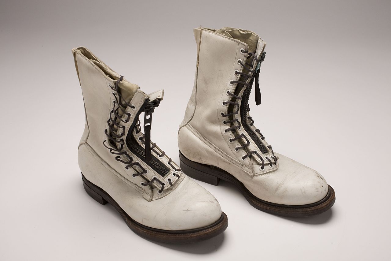
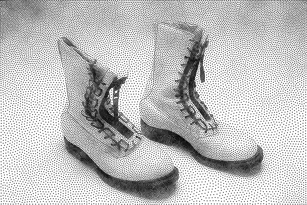
Figure 1: Stippling. According to Wikipedia, Stippling is the creation of a pattern simulating varying degrees of solidity or shading by using small dots. Such a pattern may occur in nature and these effects are frequently emulated by artists. The pair of boots (left part) have been first converted into a gray-level image and processed into a stippling figure (right part) using the weighted Voronoi stippling technique by [29] and replicated in [27]. Image from [27] (CC-BY license).

However, before studying the influence of the spatial localisation of neurons, it is necessary to design first a method for the arbitrary placement of neurons. This article introduces a graphical, scalable and intuitive method for the placement of neurons (or any other type of cells actually) over a two-dimensional manifold and provides as well the necessary information to connect neurons together using either an automatic mapping or a user-defined function. This graphical method is based on a stippling techniques originating from the computer graphics domain for non-photorealistic rendering as illustrated on figure 3.

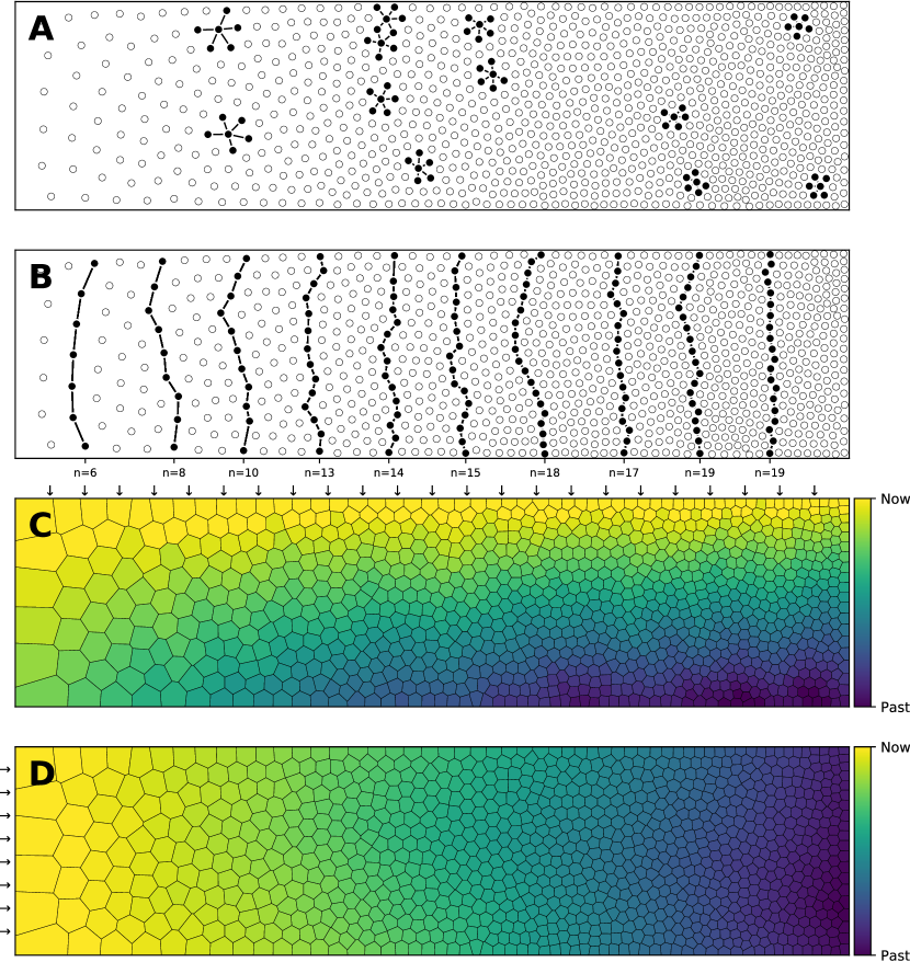
Figure 2: Influence of spatial distribution on signal propagation. A. A k-nearest neighbours (k=5) connectivity pattern shows mid-range connection lengths in low local density areas (left part) and short-range connection lengths in high density areas (right part). B. Shortest path from top to bottom using a k-nearest neighbours connectivity pattern (k=5). The lower the density, the shorter the path and the higher the density, the longer the path. On the far left, the shortest path from top to bottom is only 6 connections while this size triples on the far right to reach 19 connections. Said differently, the left part is the fast pathway while the right part is the slow pathway relatively to some input data that would feed the architecture from the top. C. Due to the asymmetry of cells position, a signal entering on the top side (materialized with small arrows) travels at different speeds and will consequently reach the bottom side at different times. This represents a spatialization of time. D. Due to the asymmetry of cells position, a signal entering on the left side (materialized with small arrows) slows down while traveling before reaching the right side. This represents a compression of time and may serve as a short-term working memory.

2 Methods

Blue noise [31] is an even, isotropic yet unstructured distribution of points [22] and has minimal low frequency components and no concentrated spikes in the power spectrum energy [35]. Said differently, blue noise (in the spatial domain) is a type of noise with intuitively good properties: points are evenly spread without visible structure (see figure 3 for the comparison of a uniform distribution and a blue noise distribution). This kind of noise has been extensively studied in the computer graphic domain and image processing because it can be used for object distribution, sampling, printing, half-toning, etc. One specific type of spatial blue noise is the Poisson disc distribution that is a 2D uniform point distribution in which all points are separated from each other by a minimum radius (see right part of figure 3). Several methods have been proposed for the generation of such noise, from the best in quality (dart throwing [8]) to faster ones (rejection sampling [6]), see [18] for a review. An interesting variant of the Poisson disk distribution is a non isotropic distribution where local variations follow a given density function as illustrated on figure 3 where the density function has been specified using the image gray levels. On the stippling image on the right, darker areas have a high concentration of dots (e.g. boots sole) while lighter areas such as the background display a sparse number of dots. There exist several techniques for computing such stippling density-driven pattern (optimal transport [22], variational approach [7], least squares quantization [19], etc.) but the one by [29] is probably the most straightforward and simple and has been recently replicated in [27].

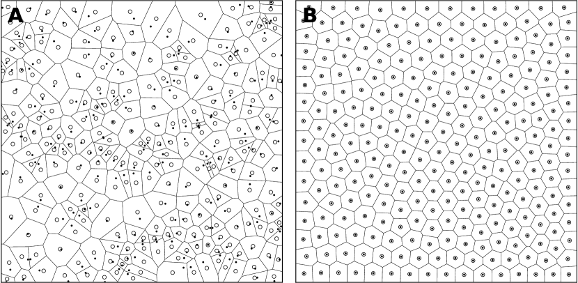
Figure 3: Centroidal Voronoi Tesselation. A. Voronoi diagram of a uniform distribution (n=256) where black dots represent the uniform distribution and white circles represent the centroids of each Voronoi cells. B. Centroidal Voronoi diagram where the point distribution matches the centroid distribution.

2.1 Distribution

The desired distribution is given through a bitmap RGBA image that provides two types of information. The three color channels indicates the identity of a cell (using a simple formula of the type $identity=256\times 256\times R+256\times G+B$ for $0\leq R,G,B<256$) and the alpha channel indicates the desired local density. This input bitmap has first to be resized (without interpolation) such that the mean pixel area of a Voronoi cell is 500 pixels. For example, if we want a final number of 1000 cells, the input image needs to be resized such that it contains at least 500x1000 pixels. For computing the weighted centroid, we apply the definition proposed in [29] over the discrete representation of the domain and use a LLoyd relaxation scheme.

$${\bf C}_{i}=\frac{\int_{A}{\bf x}\rho({\bf x})dA}{\int_{A}\rho({\bf x})}$$

More precisely, each Voronoi cell is rasterized (as a set of pixels) and the centroid is computed (using the optimization proposed by the author that allow to avoid to compute the integrals over the whole set of pixels composing the Voronoi cell). As noted by the author, the precision of the method is directly related to the size of the Voronoi cell. Consequently, if the original density image is too small relatively to the number of cells, there might be quality issues. We use a fixed number of iterations ($n=50$) instead of using the difference in the standard deviation of the area of the Voronoi regions as proposed in the original paper. Last, we added a threshold parameter that allows to perform a pre-processing of the density image: any pixel with an alpha level above the threshold is set to the threshold value before normalizing the alpha channel. Figure 4 shows the distribution of four populations with respective size 1000, 2500, 5000 and 10000 cells, using the same linear gradient as input. It is remarkable to see that the local density is approximately independent of the total number of cells.

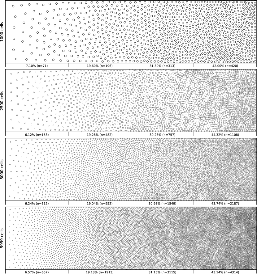
Figure 4: Non-uniform distribution (linear gradient). Different population distribution (size of 1000, 2500, 5000 and 10000 cells) using the same linear gradient as input have been computed. Each distribution has been split into four equal areas and the respective proportion and number of cells present in the area is indicated at the bottom of the area. The proportion of cells present in each areas is approximately independent ($\pm$2.5%) of the overall number of cells.

2.2 Connection

Most computational models need to define the connectivity between the different populations that compose the model. This can be done by specifying projections between a source population and a target population. Such projections correspond to the axon of the source neuron making a synaptic contact with the dendritic tree of the target neuron. In order to define the overall model connectivity, one can specify each individual projection if the model is small enough (a few neurons). However, for larger models (hundreds, thousands or millions of neurons), this individual specification would be too cumbersome and would hide any structure in the connectivity scheme. Instead, one can use generic connectivity description [11] such as one-to-one, one-to-all, convergent, divergent, receptive fields, convolutional, etc. For such connectivity scheme to be enforced, it requires either a well structured populations (e.g. grid) or a simple enclosing topology [26] such as a rectangle or a disc. In the case of arbitrary shapes as shown on figure 5, these methods cannot be used directly. However, we can use an indirect mapping from a reference shape such as the unit disc and take advantage of the Riemann mapping theorem that states (definition from [5]):

Riemann mapping theorem (from [5]). Let $\Omega$ be a (non empty) simply connected region in the complex plane that is not the entire plane. Then, for any $z_{0}\in\Omega$, there exists a bianalytic (i.e. biholomorphic) map $f$ from $\Omega$ to the unit disc such that $f(z0)=0$ and $f^{\prime}(z0)>0$.

Such mapping is conformal, that it, it preserves angles while isometric mapping preserves lengths (developable surfaces) and equiareal mapping preserves areas. [17] introduced a method to compute the Riemann mapping function using the Szegö kernel that is numerically stable while [30] introduced numerical methods for solving the more specific conformal Schwarz-Christoffel transformation (conformal transformation of the upper half-plane onto the interior of a simple polygon). Furthermore, a Matlab toolkit is available in [12] as well as a Python translation (https://github.com/AndrewWalker/cmtoolkit) that has been used to produce the figure 5 that shows some examples of arbitrary shapes and the automatic mapping of the polar and Cartesian domains.

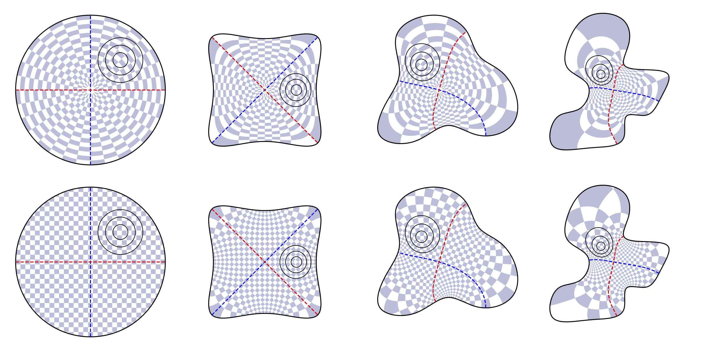
Figure 5: Conformal mappings. Examples of conformal mappings on arbitrary spline shapes using the conformal Riemann mapping via the Szegö kernel [17]. Top line shows conformal mapping of the polar domain, bottom line show conformal mapping of the Cartesian domain.

However, even if automatic, this mapping can be perceived as not intuitive. Provided the shape are not too distorted, we’ll see in the results section that ad-hoc mapping can also be used.

2.3 Visualization

Having now a precise localization for each cell of each population, we have several ways of visualizing the activity within the model. The most straightforward way is to simply draw the activity of a cell at its position using a disc of varying color (a.k.a. colormap) or varying size, correlated with cell activity. This requires the total number of cells to be not too large or the display would be cluttered. For a moderate number of cells, we can take advantage of the dual Voronoi diagram of the cell position as illustrated on figure 2, using a colormap to paint the Voronoi cell. Finally, if the number of cells is really high, A two-dimensional histogram of the mean activity (with a fixed number of bins) can be used as shown on figure 8C using a bicubic interpolation filter.

3 Results

We’ll now illustrate the use of the proposed method on three different cases.

3.1 Case 1: Retina cells

The human retina counts two main types of photoreceptors, namely rods, and cones (L-cones, M-cones and S-cones). They are distributed over the retinal surface in an non uniform way, with a high concentration of cones (L-cones and M-cones) in the foveal region while the rods are to be found mostly in the peripheral region with a peak density at around 18-20^∘ of foveal eccentricity. Furthermore, the respective size of those cells is different, rods being much smaller than cones. The distribution of rods and cells in the human retina has been extensively studied in the literature and is described precisely in a number of work [10, 1]. Our goal here is not to fit the precise distribution of cones and rods but rather to give a generic procedure that can be eventually used to fit those figures, for a specific region of the retina or the whole retina. The main difficulty is the presence of two types of cells having different sizes. Even though there exist blue-noise sampling procedures taking different size into account [35], we’ll use instead the aforementioned method using a two stage procedure as illustrated on figure 6.

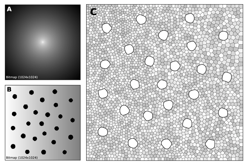
Figure 6: Cones and rods distribution. A. The density map for cones placement (n=25) is a circular and quadratic gradient with highest density in the center. B. The density map for rods placement (n=2500) is built using the rods distribution. Starting from a linear density, “holes” with different sized are created at the location of each cone, preventing rods to spread over these areas during the stippling procedure. C. Final distribution of cones and rods. Cones are represented as white blobs (splines) while rods are represented as Voronoi regions using random colors to better highlight the covered area.

A first radial density map is created for the placement of 25 cones and the stippling procedure is applied for 15 steps to get the final positions of the 25 cones. A linear rod density map is created where discs of varying (random) sizes of null density are created at the position of the cones. These discs will prevent the rods to spread over these areas. Finally, the stippling procedure is applied a second time over the built density map for 25 iterations. The final result can be seen on figure 6C where rods are tightly packed on the left, loosely packed on the left and nicely circumvent the cones.

3.2 Case 2: Neural field

Neural fields describe the dynamics of a large population of neurons by taking the continuum limit in space, using coarse-grained properties of single neurons to describe the activity [34, 33, 2, 9]. In this example, we consider a neural field with activity $u$ that is governed by an equation of the type:

$$\tau\frac{\partial u(x,t)}{\partial t}=-u(x,t)+\int_{-\infty}^{+\infty}w(x,y)f(u(y,t))dy+I(x)+h$$

The lateral connection kernel $w$ is a difference of Gaussian (DoG) with short range excitation and long range inhibition and the input $I(x)$ is constant and noisy. In order to solve the neural field equation, the spatial domain has been discretized into $40\times 40$ cells and the temporal resolution has been set to $10ms$. On figure 7A, one can see the characteristic Turing patterns that have formed within the field. The number and size of clusters depends on the lateral connection kernel. Figure 7B shows the discretized and homogeneous version of the DNF where each cell has been assigned a position on the field, the connection kernel function and the parameters being the same as in the continuous version. The result of the simulation shown on figure 7B is the histogram of cell activities using $40\times 40$ regular bins. One can see the formation of the Turing patterns that are similar to the continuous version. On figure 7C however, the position of the cells have been changed (using the proposed stippling method) such that there is a torus of higher density. This is the only difference with the previous model. While the output can still be considered to be Turing patterns, one can see clearly that the activity clusters are precisely localized onto the higher density regions. Said differently, the functional properties of the field have been modified by a mere change in the structure. This tends to suggest that the homogeneous condition of neural fields (that is the standard hypothesis in most works because it facilitates the mathematical study) is actually quite a strong limitation that constrains the functional properties of the field.

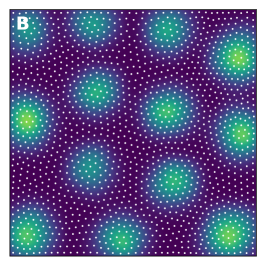
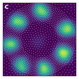
Figure 7: Non-homogeneous discrete neural field. A. Turing patterns resulting from a continuous and homogeneous neural field with constant and noisy input. B. Turing patterns resulting from a discrete and homogeneous neural field with constant and noisy input. White dots indicate the position of the cells. Mean activity is compute from the histogram of cells activity using $40\times 40$ bins. C. Localized Turing patterns resulting from a discrete and non-homogeneous neural field with constant and noisy input. White dots indicate the position of the cells. Mean activity is computed from the histogram of cells activity using $40\times 40$ bins.

3.3 Case 3: Basal ganglia

The basal ganglia is a group of sub-cortical nuclei (striatum, globus pallidus, subthamalic nucleus, subtantia nigra) associated with several functions such as motor control, action selection and decision making. There exists a functional dissociation of the ventral and the dorsal part of the striatum (caudate, putamen and nucleus accumbens) that is believed to play an important role in decision making [24, 3, 21] since these two regions do not receive input from the same structures. For a number of models, this functional dissociation results in the dissociation of the striatum into two distinct neural groups even though such anatomical dissociation does not exist per se (see [14]). Without any proper topography of the striatal nucleus, it is probably the most straightforward way to proceed. However, if each group would possess its own topography, it would become possible to distinguish the ventral from the dorsal part of the BG, as illustrated on figure 8 on a coronal view of the BG. We do not pretend this simplified view is sufficient to give account on all the intricate connections between the different nuclei composing the basal ganglia, but it might nonetheless help to have better understanding of the structure because it becomes possible to link external input to specific part of this or that structure (eg. ventral or dorsal part of the striatum). This could lead to differential processing in different part of the striatum and may reconcile different theories regarding the role of the ventral and the dorsal part.

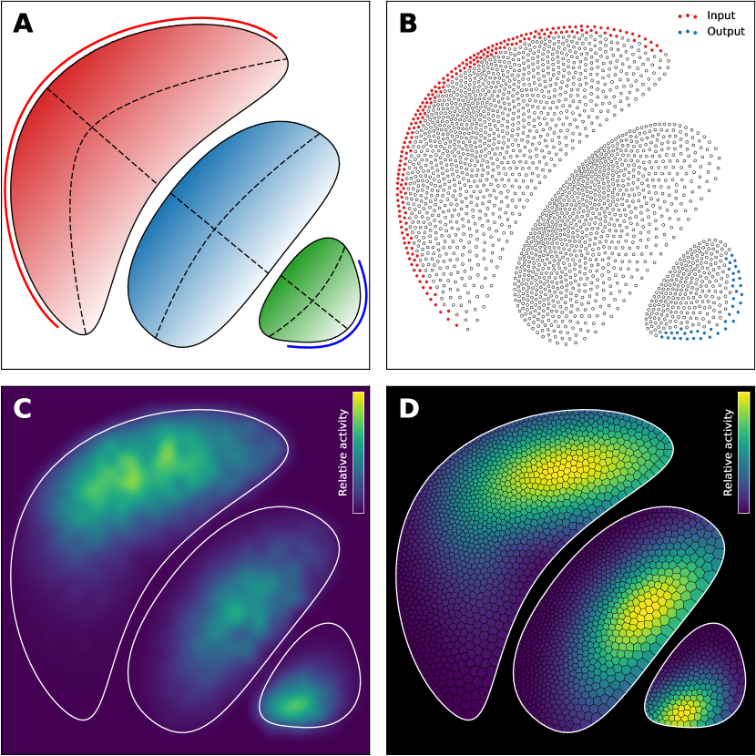
Figure 8: Coronal view of the basal ganglia. A. Scalable Vector Graphic (SVG) source file defining each structure in terms of border (solid black lines), major and minor axis (dashed lines), input (red line) and output (blue line). Local density is given by the alpha channel and structure identity is given by the color. In this coronal view of the basal ganglia, the Caudate is red (RGB=(0.83,0.15,0.15)), the GPe is blue (RGB=(0.12,0.46,0.70)) and the GPi is green (RGB=(0.17,0.62,0.17)). B. Distribution of 2500 neurons respecting the local density and structural organization (Caudate: 1345 cells, GPe: 884 cells, GPi: 271 cells). Neurons receiving input are drawn in red, neurons sending output are drawn in blue. Each neuron possesses two set of coordinates: one global Cartesian coordinate set and a local curvilinear coordinates set defined as the distances to the major and the minor axis of the structure the neuron belongs to. C. Mean activity histogram of the different structures using 32x32 bins and a bi-cubic interpolation filter. Each bin includes from zero to several neurons. D. Cell activities represented using the dual Voronoi diagram of the cell position. Each Voronoi region is painted according to the activity of the corresponding centroid (i.e. neuron).

4 Discussion

We’ve introduced a graphical, scalable and intuitive method for the placement and the connection of biological cells and we illustrated its use on three use-cases. We believe this method, even if simple and obvious, might be worth to be considered in the design of a new class of model, in between symbolic model and realistic model. Our intuition is that such topography may be an important aspect that needs to be taken into account and studied in order for the model to benefit from structural functionality. Furthermore, the proposed specification of the architecture as an SVG file associated with the scalability of the method could guarantee to some extent the scalability of the properties of the model.

Notes: All figures were produced using the Python scientific stack, namely, SciPy [16], Matplotlib [15] and NumPy [32]. All sources are available on GitHub [28]

References

- [1] Peter K Ahnelt and Helga Kolb “The mammalian photoreceptor mosaic-adaptive design” In Progress in Retinal and Eye Research 19.6 Elsevier BV, 2000, pp. 711–777 DOI: 10.1016/s1350-9462(00)00012-4
- [2] Shun-Ichi Amari “Dynamics of pattern formation in lateral-inhibition type neural fields” In Biological Cybernetics 27.2 Springer Nature, 1977, pp. 77–87 DOI: 10.1007/bf00337259
- [3] B.. Balleine, M.. Delgado and O. Hikosaka “The Role of the Dorsal Striatum in Reward and Decision-Making” In Journal of Neuroscience 27.31 Society for Neuroscience, 2007, pp. 8161–8165 DOI: 10.1523/jneurosci.1554-07.2007
- [4] Lidia Blazquez-Llorca et al. “Spatial distribution of neurons innervated by chandelier cells” In Brain Structure and Function 220.5 Springer Nature, 2014, pp. 2817–2834 DOI: 10.1007/s00429-014-0828-3
- [5] Michael Bolt, Sarah Snoeyink and Ethan Van Andel “Visual representation of the Riemann and Ahlfors maps via the Kerzman–Stein equation” In Involve, a Journal of Mathematics 3.4 Mathematical Sciences Publishers, 2010, pp. 405–420 DOI: 10.2140/involve.2010.3.405
- [6] Robert Bridson “Fast Poisson disk sampling in arbitrary dimensions” In ACM SIGGRAPH 2007 sketches on - SIGGRAPH ’07 ACM Press, 2007 DOI: 10.1145/1278780.1278807
- [7] Zhonggui Chen et al. “Variational Blue Noise Sampling” In IEEE Transactions on Visualization and Computer Graphics 18.10 Institute of ElectricalElectronics Engineers (IEEE), 2012, pp. 1784–1796 DOI: 10.1109/tvcg.2012.94
- [8] Robert L. Cook “Stochastic sampling in computer graphics” In ACM Transactions on Graphics 5.1 Association for Computing Machinery (ACM), 1986, pp. 51–72 DOI: 10.1145/7529.8927
- [9] “Neural Fields” Springer Berlin Heidelberg, 2014 DOI: 10.1007/978-3-642-54593-1
- [10] Christine A. Curcio, Kenneth R. Sloan, Robert E. Kalina and Anita E. Hendrickson “Human photoreceptor topography” In The Journal of Comparative Neurology 292.4 Wiley-Blackwell, 1990, pp. 497–523 DOI: 10.1002/cne.902920402
- [11] Mikael Djurfeldt, Andrew P. Davison and Jochen M. Eppler “Efficient generation of connectivity in neuronal networks from simulator-independent descriptions” In Frontiers in Neuroinformatics 8 Frontiers Media SA, 2014 DOI: 10.3389/fninf.2014.00043
- [12] Tobin A. Driscoll “Algorithm 756, a MATLAB toolbox for Schwarz-Christoffel mapping” In ACM Transactions on Mathematical Software 22.2 Association for Computing Machinery (ACM), 1996, pp. 168–186 DOI: 10.1145/229473.229475
- [13] Donald O. Hebb “The Organization of Behavior: a Neuropsychological Theory” New York: Wiley, 1949
- [14] Mark D. Humphries and Tony J. Prescott “The ventral basal ganglia, a selection mechanism at the crossroads of space, strategy, and reward.” In Progress in Neurobiology 90.4 Elsevier BV, 2010, pp. 385–417 DOI: 10.1016/j.pneurobio.2009.11.003
- [15] J.. Hunter “Matplotlib: A 2D graphics environment” In Computing In Science & Engineering 9.3 IEEE COMPUTER SOC, 2007, pp. 90–95 DOI: 10.1109/MCSE.2007.55
- [16] Eric Jones, Travis Oliphant and Pearu Peterson “SciPy: Open source scientific tools for Python”, 2001 URL: http://www.scipy.org
- [17] Norberto Kerzman and Manfred R. Trummer “Numerical conformal mapping via the Szegö kernel” In Journal of Computational and Applied Mathematics 14.1-2 Elsevier BV, 1986, pp. 111–123 DOI: 10.1016/0377-0427(86)90133-0
- [18] Ares Lagae and Philip Dutré “A Comparison of Methods for Generating Poisson Disk Distributions” In Computer Graphics Forum 27.1 Wiley-Blackwell, 2008, pp. 114–129 DOI: 10.1111/j.1467-8659.2007.01100.x
- [19] S. Lloyd “Least squares quantization in PCM” In IEEE Transactions on Information Theory 28.2 Institute of ElectricalElectronics Engineers (IEEE), 1982, pp. 129–137 DOI: 10.1109/tit.1982.1056489
- [20] B.H. McCormick, R.W. DeVaul, W.R. Shankle and J.H. Fallon “Modeling neuron spatial distribution and morphology in the developing human cerebral cortex” In Neurocomputing 32-33 Elsevier BV, 2000, pp. 897–904 DOI: 10.1016/s0925-2312(00)00258-7
- [21] Matthijs AA Meer and A David Redish “Ventral striatum: a critical look at models of learning and evaluation” In Current Opinion in Neurobiology 21.3 Elsevier BV, 2011, pp. 387–392 DOI: 10.1016/j.conb.2011.02.011
- [22] Soham Uday Mehta, Brandon Wang and Ravi Ramamoorthi “Axis-aligned filtering for interactive sampled soft shadows” In ACM Transactions on Graphics 31.6 Association for Computing Machinery (ACM), 2012, pp. 1 DOI: 10.1145/2366145.2366182
- [23] Bhargav Teja Nallapu, Bapi Raju Surampudi and Nicolas P. Rougier “The art of scaling up : A computational account on action selection in basal ganglia” In 2017 International Joint Conference on Neural Networks (IJCNN) IEEE, 2017 DOI: 10.1109/ijcnn.2017.7965835
- [24] J. O’Doherty “Dissociable Roles of Ventral and Dorsal Striatum in Instrumental Conditioning” In Science 304.5669 American Association for the Advancement of Science (AAAS), 2004, pp. 452–454 DOI: 10.1126/science.1094285
- [25] Joseph F. Pasternak and Thomas A. Woolsey “The number, size and spatial distribution of neurons in Lamina IV of the mouse SmI neocortex” In The Journal of Comparative Neurology 160.3 Wiley-Blackwell, 1975, pp. 291–306 DOI: 10.1002/cne.901600303
- [26] Hans Ekkehard Plesser and Håkon Enger “NEST Topology user manual”, 2015 URL: http://www.nest-simulator.org/wp-content/uploads/2015/04/Topology_UserManual.pdf
- [27] Nicolas P. Rougier “[Re] Weighted Voronoi Stippling” In ReScience 3.1, 2017 DOI: 10.5281/zenodo.802285
- [28] Nicolas P. Rougier “Spatial Computation”, 2017 DOI: 10.5281/zenodo.1012306
- [29] Adrian Secord “Weighted Voronoi stippling” In Proceedings of the second international symposium on Non-photorealistic animation and rendering - NPAR ’02 ACM Press, 2002 DOI: 10.1145/508530.508537
- [30] Lloyd N. Trefethen “Numerical Computation of the Schwarz–Christoffel Transformation” In SIAM Journal on Scientific and Statistical Computing 1.1 Society for Industrial & Applied Mathematics (SIAM), 1980, pp. 82–102 DOI: 10.1137/0901004
- [31] Robert Ulichney “Digital Halftoning” Cambridge, MA, USA: MIT Press, 1987
- [32] Stéfan Walt, S Chris Colbert and Gaël Varoquaux “The NumPy Array: A Structure for Efficient Numerical Computation” In Computing in Science & Engineering 13.2 Institute of ElectricalElectronics Engineers (IEEE), 2011, pp. 22–30 DOI: 10.1109/mcse.2011.37
- [33] Hugh R. Wilson and Jack D. Cowan “A mathematical theory of the functional dynamics of cortical and thalamic nervous tissue” In Kybernetik 13.2 Springer Nature, 1973, pp. 55–80 DOI: 10.1007/bf00288786
- [34] Hugh R. Wilson and Jack D. Cowan “Excitatory and Inhibitory Interactions in Localized Populations of Model Neurons” In Biophysical Journal 12.1 Elsevier BV, 1972, pp. 1–24 DOI: 10.1016/s0006-3495(72)86068-5
- [35] Sen Zhang et al. “Capacity constrained blue-noise sampling on surfaces” In Computers & Graphics 55 Elsevier BV, 2016, pp. 44–54 DOI: 10.1016/j.cag.2015.11.002