Fingerprints of spin-orbital polarons and of their disorder
in the photoemission spectra of doped Mott insulators with orbital degeneracy

Abstract

We explore the effects of disordered charged defects on the electronic excitations observed in the photoemission spectra of doped transition metal oxides in the Mott insulating regime by the example of the $R_{1-x}$Ca_xVO₃ perovskites, where $R=$ La, $\dots$, Lu. A fundamental characteristic of these vanadium $d^{2}$ compounds with partly filled $t_{2g}$ valence orbitals is the persistence of spin and orbital order up to high doping, in contrast to the loss of magnetic order in high-$T_{c}$ cuprates at low defect concentration. We demonstrate that the disordered electronic structure of doped Mott-Hubbard insulators can be obtained with high precision within the unrestricted Hartree-Fock approximation. In particular: (i) the atomic multiplet excitations in the inverse photoemission spectra and the various defect-related states and satellites are well reproduced, (ii) a robust Mott gap survives up to large doping, and (iii) we show that the defect states inside the Mott gap develop a soft gap at the Fermi energy. The soft defect states gap, that separates the highest occupied from the lowest unoccupied states, can be characterized by a shape and a scale parameter extracted from a Weibull statistical sampling of the density of states near the chemical potential. These parameters provide a criterion and a comprehensive schematization for the insulator-metal transition in disordered systems. We demonstrate that charge defects trigger small spin-orbital polarons, with their internal kinetic energy responsible for the opening of the soft defect states gap. This kinetic gap survives disorder fluctuations of defects and is amplified by the long-range $e$-$e$ interactions, whereas in the atomic limit we observe a Coulomb singularity. The small size of spin-orbital polarons is inferred by an analysis of the inverse participation ratio which explains the origin of the robustness of spin and orbital order. Using realistic parameters for the perovskite vanadate system La_1-xCa_xVO₃, we show that its soft gap is well reproduced as well as the marginal doping dependence of the position of the chemical potential relative to the center of the lower Hubbard band. The present theory uncovers also the reasons why the $d^{1}\rightarrow d^{0}$ satellite excitations, which directly probe the effect of the random defect fields on the polaron state, are not well resolved in the available experimental photoemission spectra for La_1-xCa_xVO₃.

I Introduction

In this work, we deal with transition metal oxides that are in their intrinsic state Mott insulators as a result of strong electron repulsions and not due to band structure effects as in semiconductors Imada et al. (1998); Hwang et al. (2012). Mott insulating materials typically display different realizations of quantum magnetism and some give rise to rare quantum spin liquid states Balents (2010); Sachdev and Keimer (2011); Savary and Balents (2017); Zhou et al. (2017). Doping Mott insulators can have striking consequences. For example, doping the two-dimensional (2D) antiferromagnetic (AF) Mott insulator La₂CuO₄ with Sr, Ba or Ca gives rise to high-$T_{c}$ superconductivity Lee et al. (2006); Alloul et al. (2009); Berg et al. (2011); Avella (2014), with an insulator to superconductor transition and the disappearance of AF order at very low doping Ellman et al. (1989); Khaliullin and Horsch (1993); Kastner et al. (1998). Manganites are paradigmatic examples of systems characterized by spin, orbital and charge degrees of freedom that are controlled by spin-orbital superexchange interactions Kugel and Khomskii (1982); Tokura and Nagaosa (2000); Oleś et al. (2005); Khaliullin (2005); Horsch (2007); Oleś (2012). Doping the Mott insulator LaMnO₃, for instance, leads to a variety of insulating spin-, orbital-, and charge- ordered phases Kilian and Khaliullin (1999); Feiner and Oleś (1999); Weisse and Fehske (2004); Daghofer et al. (2004); Geck et al. (2005); Oleś and Khaliullin (2011); Snamina and Oleś (1999), as well as to a metallic regime that displays a colossal magnetoresistance Dagotto et al. (2001); Dagotto (2005); Tokura (2006).

A very interesting class of materials where the orbital degree of freedom plays an important role are the $3d$-electron systems with active $t_{2g}$ degrees of freedom that drive orbital fluctuations Khaliullin (2005); De Raychaudhury et al. (2007). In the titanium perovskites, they play a prominent role in the spin-orbital order or may even trigger a disordered state Khaliullin and Maekawa (2000); Mochizuki (2002); Khaliullin and Okamoto (2003); Ishihara (2004); Cheng et al. (2008); Ulrich et al. (2015), while superconductivity was discovered at SrTiO₃ interfaces Schooley et al. (1964); Kozuka et al. (2009); Li et al. (2011); Gabay and Triscone (2013). We shall focus here on the vanadium perovskites $R$VO₃, where $R$=La,$\dots$,Lu, which reveal temperature-induced magnetization reversals Ren et al. (1998) as a result of the coupling of spin and orbital degrees of freedom of the $t_{2g}$ valence electrons Ren et al. (2000); Khaliullin et al. (2001); Horsch et al. (2003); Ulrich et al. (2003); Sirker and Khaliullin (2003); Sirker et al. (2008). This class of compounds has interesting phase diagrams with two complementary spin-orbital ordered phases and a pure orbital-ordered phase Miyasaka et al. (2003, 2006); Fujioka et al. (2010); Miyasaka et al. (2007); Sage et al. (2007); Reehuis et al. (2011); Lindfors-Vrejoiu et al. (2017). Remarkably, the $C$-type spin and $G$-type orbital ordered phase in La_1-xSr_xVO₃, Pr_1-xCa_xVO₃ and Y_1-xCa_xVO₃ is robust up to high-doping concentrations and also the metal-insulator transition takes place only at quite substantial doping Miyasaka et al. (2000); Fujioka et al. (2005, 2008); Reehuis et al. (2016). This striking robustness of the spin-orbital ordered state against doping as compared to the fragile AF state in the cuprates is one of the motivations for our work.

The combination of spin and orbital degrees of freedom triggers spin-orbital (SO) polarons Daghofer et al. (2006); Wohlfeld et al. (2009); Berciu (2009); Bieniasz et al. (2017). We shall discuss in this work why small SO polarons in the insulating regime of cubic vanadates Avella et al. (2015); Reehuis et al. (2016) are much more strongly bound to charge defects than spin polarons in high-$T_{c}$ materials Chen et al. (1991, 2009). The reduced mobility of doped holes or electrons inside the SO polarons implies a weaker screening of defect potentials by the doped charge carriers and thus provides an explanation for the shift of the insulator to metal transition towards high doping concentrations in the vanadates. Here, we shall support these conclusions by a careful analysis of the doping dependence of the density of states, i.e., relevant for photoemission (PES) and inverse photoemission (IPES). We explore the localization of defect states wave functions, the defect states gap inside the Mott-Hubbard (MH) gap, and finally the reduction of spin and orbital order and its relation to the many-body SO polaron wavefunction and their binding to defects.

The cubic vanadates represent a class of compounds with quantum fluctuating orbitals and spins, even in the absence of doping. In contrast to the manganites, the cubic vanadates have very small Jahn-Teller interactions, a consequence of the $t_{2g}$ nature of their valence electrons. Therefore, orbital occupations are not rigid even in the ordered phases, but fluctuate Khaliullin et al. (2001); Horsch et al. (2003, 2008). Several peculiar features can be traced back to orbital quantum fluctuations, such as ferromagnetism driven by orbital singlet fluctuations Khaliullin et al. (2001) and orbital Peierls dimerization Ulrich et al. (2003); Horsch et al. (2003); Sirker and Khaliullin (2003); Sirker et al. (2008). Indeed, the joint spin and orbital fluctuations are particularly strong in the ordered $C$-type AF and $G$-type alternating orbital (AO), i.e., $C$-AF/$G$-AO phase, realized in these compounds when they are doped Horsch and Oleś (2011). Furthermore, it was shown that charged defects tend to enhance orbital Peierls dimerization Horsch and Oleś (2011). An important motivation for the investigation of the cubic vanadates is a large experimental data base for these systems, which includes the phase diagrams of many undoped compounds Miyasaka et al. (2003, 2006); Fujioka et al. (2010) and their pressure dependence Bizen et al. (2012), as well as the doping dependence of the optical conductivity for several systems Fujioka et al. (2008). In this work, our focus is on the doping dependence of the PES spectra of the vanadium perovskites Maiti et al. (1998); Maiti and Sarma (2000); Pen et al. (1999).

Solving this problem involves, for example, answering questions like: (i) What is the nature of defect states in a strongly correlated system, i.e., to what extent are such defect states different from those in usual semiconductors or band insulators Gantmakher (2005); Drabold and Estreicher (2007)? (ii) What happens to the MH gap in the presence of defects? (iii) Which are the different features of defect states in MH insulators with orbital degeneracy within $t_{2g}$ transition metal oxides as compared to those in doped high-$T_{c}$ superconductors? (iv) Which methods, among those capable to yield reliable results for MH insulators, can be efficiently extended to take into account defects and disorder? To answer these questions is a formidable challenge, as defects greatly influence the subtle interplay of spin, orbital, lattice and charge degrees of freedom.

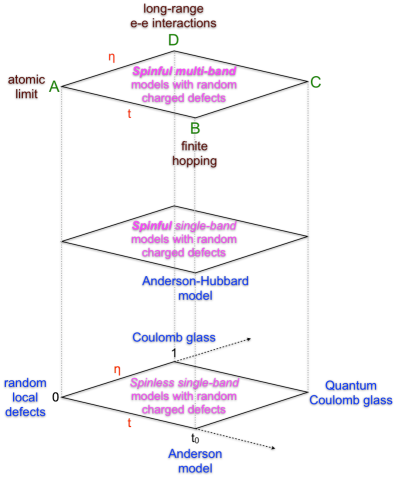
Figure 1: Schematic hierarchy of typical models for systems with disorder: On the lowest floor, generic models with a single orbital per site and no spin are shown. These models are further distinguished depending on whether they involve long-range $e$-$e$ interactions ($\eta$-scale) and/or kinetic energy ($t$-scale). By adding spin to charge carriers one finds single orbital Hubbard-type models shown on the second floor. On the third top floor, reside models with spin and orbital degrees of freedom of interest in this paper, designed for doped spin-orbital systems. The labels A, B, C, and D refer to models explained and investigated in following Sections.

The calculation of the electronic structure of a disordered system with charged defects and long-range $e$-$e$ interactions is a difficult optimization problem even for the simplest models for the defect states in the gap of semiconductors, e.g., the Coulomb glass (CG) model Gantmakher (2005). The effect of disorder and the resulting localization of electron states has a long history Anderson (1958); Lee and Ramakrishnan (1985). The reason for the calculational complexity of the insulating phase is the absence of metallic screening, and therefore the energy and occupation of a defect state depends on that of far distant random defects because of the long-range Coulomb interaction Lee and Ramakrishnan (1985). In contrast, in the metallic state, because of the presence of a Fermi surface, perturbative diagrammatic techniques can be applied to deal with multiple scattering corrections leading to a Coulomb anomaly in the density of states (DOS) $N(\omega)$ Altshuler and Aronov (1979). For the insulating phase, it was argued by Pollak Pollack (1970) that $e$-$e$ interactions should lead to a depletion of $N(\omega)$ at the chemical potential in systems with disorder. For the CG model, Efros et al. Efros and Shklovskii (1975); Efros (1976); Efros et al. (2011) could show, using some simplifying criteria, that the Coulomb interaction generates at a soft gap at the chemical potential in $N(\omega)\propto|\omega|^{\nu}$, with an exponent $\nu=d-1$ determined by the spatial dimension $d$. This is called the Coulomb gap Efros and Shklovskii (1975). Recently, Shinoaka and Imada Shinaoka and Imada (2009, 2010) reported unconventional soft gaps for models with only short-range interactions. Furthermore, a disorder-induced Coulomb or zero-bias anomaly was observed by Epperlein et al. Epperlein et al. (1997) for the quantum CG model and by Yun Song et al. Song et al. (2009) for an extended Anderson-Hubbard model.

We base our study on a generic spinful three-band model for the $t_{2g}$ electrons on the vanadium ions Avella et al. (2015) that provides a complete description of the magnetic and orbital ordered phases. The model includes the local Hubbard-Hund interactions and thereby describes the atomic multiplet structure of the V ions. Moreover, the model contains the long-range $e$-$e$ interactions, and thereby it includes the dielectric screening of the $t_{2g}$ electrons, and it contains the Coulomb potentials of the random defects. Finally, there is the flavor conserving kinetic energy of $t_{2g}$ electrons, and moreover crystal field and Jahn-Teller interactions. All these interactions together yield spin-orbital superexchange and pure orbital interactions that determine the different spin- and orbital ordered phases Khaliullin et al. (2001); Horsch et al. (2008). This model can be simplified by the elimination of degrees of freedom and by the removal of terms, such as the kinetic energy or the Hubbard interaction for instance, to obtain simpler models that have been used in the study of disorder. For instance, one may arrive at the CG Efros and Shklovskii (1975) or at the quantum CG Pollack (1970); Epperlein et al. (1997) models after elimination of spin and orbital degrees of freedom, or at the Anderson-Hubbard model Shinaoka and Imada (2009) after elimination of the orbital degrees of freedom (see Fig. 1).

It requires highly efficient methods like the Hartree, the Hartree-Fock Mizokawa et al. (2000); Barreteau et al. (2000); Chen et al. (2009); Schickling et al. (2011a); Horsch and Oleś (2011), or the density functional method Solovyev (2008); Carrasco et al. (2006); Pavlenko et al. (2012) to analyze systems with defects and disorder. Besides disorder, the calculations of the electronic structure and excitations of the spinful multiband models with charged defects are complicated by the fact that our systems are Mott insulators. We have already demonstrated that the Hartree-Fock method is also capable to describe faithfully the atomic multiplet structure in the spin-orbital degenerate case provided the system has a broken spin and orbital symmetry and one can apply the unrestricted Hartree Fock (uHF) version of the method Horsch and Oleś (2011); Avella et al. (2013). In presence of local off-diagonal terms, the Hubbard-Hund interaction has to be expressed in rotational invariant form in spin and orbital space. The uHF method Mizokawa and Fujimori (1995, 1997); Weng and Terakura (2010), is known to be reliable for systems with spontaneously broken symmetries as, for instance, multiband models for manganites Mizokawa et al. (2000); Solovyev (2009), or the iron-based superconductors Kubo and Thalmeier (2009); Schickling et al. (2011b); Luo et al. (2013); Luo and Dagotto (2014) or clusters of transition metals with magnetic ground states Barreteau et al. (2000). The uHF method designed and used in this paper is capable to treat simultaneously phenomena that arise at distinct energy scales: the high energy scale of $\sim 1$ eV related to the (on-site and intersite) Coulomb interactions in proximity of the defects and the low energy scale of $\sim 0.1$ eV that is characteristic of the orbital physics and controls the electronic transport in doped materials. Accordingly, the method is able to address the onset of the orbital order and its remarkable robustness in doped La_1-xSr_xVO₃ and Y_1-xCa_xVO₃.

Figure 2 displays PES and IPES data of Maiti and Sarma Maiti and Sarma (2000) for the undoped reference compound LaVO₃. The data provides evidence that the system is a Mott insulator. One recognizes the LHB in PES and one also sees the UHB in IPES, where the theoretically expected multiplet bands have some correspondence with features in the experiment. The fact that the Hubbard gap in the vicinity of $\omega=0$ appears as a soft gap suggests that the sample contained possibly some defects at the surface Chen et al. (2009). The experimental data is compared with the uHF calculation, where the DOS $N(\omega)$ is broadened with an extra linewidth of $\gamma=0.5$ eV. This has the consequence that the multiplets of the UHB are no longer resolved in the theoretical DOS $N(\omega)$.

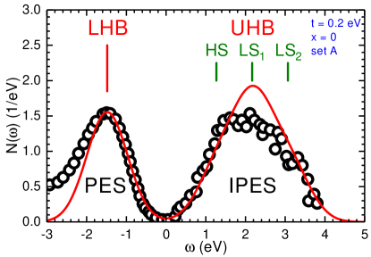
Figure 2: Photoemission (PES) and inverse photoemission (IPES) spectra for undoped LaVO₃ in the vicinity of the chemical potential, which is located at $\omega=0$. Experimental data (black hollow circles) were obtained by Maiti and Sarma Maiti and Sarma (2000); the solid (red) curve was obtained from the theory reported in Sec. IV, with the three peaks of the UHB marked as HS, LS₁, and LS₂ standing for the high-spin and the two low-spin excitations, respectively.

A surprising feature of the electronic structure of cubic vanadates is the persistence of the MH gap up to high doping concentrations Horsch and Oleś (2011). This has been demonstrated most clearly by optical conductivity experiments Fujioka et al. (2008) in La_1-xSr_xVO₃ and Y_1-xCa_xVO₃ for doping concentrations up to $x=0.1$ and 0.17, respectively. Our uHF calculations of the statistically averaged DOS $N(\omega)$ reproduces this robustness of the MH bands beyond doping concentrations of 50%, despite the fact that substantial spectral weight is transferred from the Hubbard bands to defect states. The latter appear as satellites and as states inside the MH gap. We shall discuss the energetics of these states, the sum rules and the spectral weight transfers.

Our main focus is on the defect states that appear in the MH gap and that themselves form a defect states (DS) gap at the chemical potential. The DS gap depends both on the kinetic energy parameter $t$ and the $e$-$e$ interactions strength which we can tune with a coupling constant $\eta\in[0,1]$, where $\eta=0$ corresponds to the absence of $e$-$e$ interactions and $\eta=1$ to the estimated typical strength for these interactions in vanadates. We perform a statistical analysis of the power law behavior of the DS gap in the DOS $N(\omega)\propto|\omega|^{\nu}$ in the vicinity of of the chemical potential. The exponent $\nu$ is nonuniversal and depends on $t$ and $\eta$. It has been shown that the kinetic energy of the $t_{2g}$ electrons plays a fundamental role for the formation of the DS gap in the cubic vanadates Avella et al. (2015). This mechanism is distinct from the Coulomb gap mechanism. We furthermore show that, with increasing $\eta$, $e$-$e$ interactions of Coulomb type do increase the DS gap. Yet in the atomic limit, that is without kinetic energy ($t=0$), we found that $e$-$e$ interactions alone are not strong enough in the cubic vanadates to open a Coulomb gap.

We investigate the localization of defect states by means of the inverse participation number (IPN) Bell and Dean (1970); Thouless (1974); Wegner (1980). We have generalized this concept here to the case with spin- and orbital- degeneracy. We find that at moderate doping, all wave functions are well localized. The states in the Hubbard bands are less localized than the defect states inside the Mott gap that contribute to the soft gap. These states are typically localized on 1-2 sites with tiny admixtures from further neighbors. Interestingly, we observe a discontinuity in the localization of the wave functions below and above the chemical potential when $e$-$e$ interactions are switched on. The small participation number ($<2$) for the doped hole states can be taken as an unambiguous sign that holes are in small spin-orbital polaron states that are strongly bound to the charge defects, i.e., basically on a single bond. This leads to a reduction of spatial symmetry Avella et al. (2015). The strong localization of wave functions appears consistent with experiments by Nguyen and Goodenough Nguyen and Goodenough (1995) who analyzed the magnetic properties of the La_1-xCa_xVO₃ system, and who concluded that carriers are in trapped small polaron states. Moreover, in a recent combined x-ray and neutron diffraction study of Pr_1-xCa_xVO₃, Reehuis et. al. Reehuis et al. (2016) found signatures for spin-orbital polarons from the change of spin and orbital correlations close to the insulator-metal transition at $x\simeq 0.23$.

In PES experiments of gapped systems, the position of the chemical potential $\mu$ is a subtle issue as it is determined by defects Damascelli et al. (2003); Comin and Damascelli (2016). For the doped cubic vanadates, we find that $\mu$ lies in the center of the DS states gap that forms inside the MH gap. We find that the distance of $\mu$ from the center of the LHB scales with the binding strength of the Ca defect and is basically unchanged by doping up to 50%, consistent with the PES study of Maiti and Sarma Maiti et al. (1998); Maiti and Sarma (2000) for La_1-xCa_xVO₃. We interpret this as manifestation of small polaron physics. Furthermore, we show that $d^{1}\rightarrow d^{0}$ satellites in PES spectra can provide a precise fingerprint of the state of spin-orbital polarons and the strength and variance of the random defect fields acting on it.

The paper is organized as follows. In Sec. II, we introduce the triply degenerate Hubbard model for $t_{2g}$ electrons in the doped perovskite vanadates, such as La_1-xCa_xVO₃ with Ca²⁺ charged defects replacing randomly some La³⁺ ions. The model includes local (on-site) and long-range Coulomb interactions, as well as the Coulomb potentials induced by Ca defects, which increase the energies of the $t_{2g}$ electrons located close to the defects taking also into account the contributions of more distant defects at random positions. We treat the $e$-$e$ interactions in the uHF approximation and consider two parameter sets for La_1-xCa_xVO₃ motivated by the experimental data in Sec. III. Using this approach and performing self-consistent calculations for realistic $t_{2g}$ hopping integral, $t=0.2$ eV, we obtained the one-particle DOSs presented in Sec. IV.1. They are interpreted using the generic structure of the PES and IPES spectra in a doped system with orbital degeneracy derived from the atomic limit in Sec. IV.2. We analyze the multiplet structure and comment on the PES and IPES data obtained for the undoped LaVO₃ Maiti and Sarma (2000). The numerical spectral weights near the atomic limit confirm the exact calculations, as shown in Sec. IV.3. Furthermore, using the results simulating the atomic limit (i.e., for a very low value of the hopping integral $t=0.01$ eV) we extract the effects that arise due to finite kinetic energy and emphasize the role played by active bonds in Sec. IV.4. While the excitations for the active bonds can be resolved from the spectra, we also analyze the sum rules obeyed by the structures seen in the PES. In Sec. V, we elucidate the kinetic mechanism of the gap in the present system and perform the Weibull analysis Avella et al. (2015). The electronic states that contribute to the spectral functions have various degrees of localization, which is universal for various defect realizations, as we show in detail in Sec. VI. Actually, more localized states appear at the edges of Hubbard bands. In Sec. VII, we explain gradual changes of spin-orbital order with increasing doping within the polaron picture. Finally, in Sec. VIII, we briefly address the experimental results for PES and IPES in doped systems and demonstrate that the large defect potential is responsible for the overall scenario consistent with the experiments. The final discussion and summary are presented in Sec. IX. The technical details of the present calculations are reported in two appendices: in Appendix A one finds a general discussion of the algorithm for a system with random defects, while in Appendix B it is explained what one can learn by a perturbative analysis in terms of spin-orbital polarons.

II Mott insulator with charged defects

We shall describe the doped $R_{1-x}$Ca_xVO₃ compounds (here $R$ stands either for yttrium Y or for lanthanum La) by means of a multiband Hubbard model describing the subspace of $t_{2g}$-states at vanadium ions. Previous studies Khaliullin (2005); Khaliullin et al. (2001); Horsch et al. (2003); Khaliullin et al. (2004); Horsch (2007) have shown that $t_{2g}$ orbitals are crucial for the description of the perovskite vanadates as Mott insulators. Each dopant – calcium Ca²⁺ ions randomly replacing Y³⁺ or La³⁺ones in this specific case – is equivalent to an effective charged defect sourcing a long range Coulomb potential. The degree of randomness of the dopants’ locations is controlled, in principle, by the annealing procedure used (or not used: full randomness as in the case we analyze here) during the fabrication of the samples and leads to a quite general disorder problem in the Mott insulating regime. The sequence of terms in the following Hamiltonian is selected to highlight the crucial role played by the charged defects and the long-ranged $e$-$e$ interaction in the present system Avella et al. (2015),

$${\cal H}_{t_{2g}} =\sum_{i}h_{i}n_{i}+\frac{1}{2}\sum_{i\neq j}V_{ij}n_{i}n_{j}$$

$$+{\cal H}_{{\rm kin}}+{\cal H}_{{\rm int}}+{\cal H}_{\mathrm{CF}}+{\cal H}_{\mathrm{JT}},$$ (1)

where $n_{i}=\sum_{\alpha\sigma}n_{i\alpha\sigma}$ and $n_{i\alpha\sigma}=d_{i\alpha\sigma}^{\dagger}d_{i\alpha\sigma}$ are the electron density operator and the partial electron density operator for orbital $\alpha$ and spin $\sigma=\uparrow,\downarrow$, respectively, at site $i$ of a cubic Bravais lattice.

If we would restrict the Hamiltonian (1) to the single-orbital case, the first two terms would represent the CG model Efros and Shklovskii (1975) with randomly distributed local levels $\{h_{i}\}$ and long-range $e$-$e$ interactions of Coulomb type. A very important difference though between the model we propose and those usually encountered in the literature resides in the realization of the disorder: We use a fully random distribution of charged defects leading to a realistic distribution of energy levels that depends on the analyzed crystal structure and on the level of doping, and is very structured, that is, very far from the uniform or Gaussian distributions usually used [see Fig. (14)]. The additional inclusion of a nearest neighbor hopping term would lead to the quantum CG Pollack (1970); Epperlein et al. (1997). Without long-range $e$-$e$ interactions, but with a finite nearest neighbor hopping term between random levels, one would instead get the Anderson model, see Fig. 1. The strongly correlated cousins of these models involve in addition the local Hubbard interaction between electrons with opposite spins that could lead to the opening of a Mott gap. One representative model of this class is the Anderson-Hubbard model Shinaoka and Imada (2009) that belongs to the next level of sophistication in the hierarchy of models with disorder, see Fig. 1.

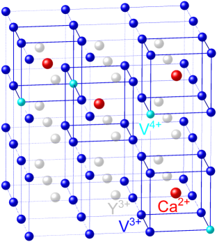
Figure 3: Cubic vanadium lattice of the doped perovskite vanadate compound $R_{1-x}$Ca_xVO₃ with random Ca²⁺ defects replacing Y³⁺ ions (O-ions are not shown). Doped holes occupy V⁴⁺ ions in the cubic V³⁺ lattice and are attracted by the Ca²⁺ ions on the cubes surrounding the defects.

As we shall see below in greater detail than what already announced above, crucial to our analysis are the random fields,

$$h_{i}=\sum_{m}V_{im}^{{\rm D}},$$ (2)

due to the electron-defect interaction $V_{im}^{{\rm D}}$, where $m$ runs over the random defect sites that are located in the center of the Vanadium cubes, see Fig. 3, and the $e$-$e$ interaction $V_{ij}$. These interactions are screened by the dielectric constant $\epsilon_{c}$ of the core electrons and depend on the distance $r$ through the function,

$$v(r)=\frac{e^{2}}{\epsilon_{c}\,r}\equiv V_{D}\,\frac{d}{r}.$$ (3)

The contribution of the $t_{2g}$ states to the screening of the interactions is not considered in the determination of $\epsilon_{c}$, but it is included explicitly in the Hamiltonian (1). A typical value for the core dielectric constant of the perovskite vanadates is $\epsilon_{c}\simeq 5$ Tsvetkov et al. (2004). In the following, we shall consider the potential energy $V_{{\rm D}}\equiv e^{2}/\epsilon_{c}\,d$ as an independent parameter, instead of $\epsilon_{c}$. Here $d=\sqrt{3}a$ is the distance between the defect ion and its closest vanadium neighbors and $a$ is the vanadium cubic lattice constant, i.e., the distance between the closest vanadium ions (see Fig. 3).

The screened interaction $v(r)$ (3) defines both the $e$-$e$ interaction and the defect potential in case of defects with a net charge of one as in the present case, i.e.,

$$V_{im}^{{\rm D}}=v(r_{im}),\quad V_{ij}=\eta v(r_{ij}),$$ (4)

where $r_{im}$ and $r_{ij}$ represent the distances between a V ion at site $i$ and a Ca defect at site $m$ ($r_{im}$) or another V ion at site $j$ ($r_{ij}$), respectively. We have introduced the parameter $\eta\in[0,1]$ in $V_{ij}$ in Eq. (4) in order to to explore the importance of $e$-$e$ interactions and the resulting dielectric screening through the $t_{2g}$ electrons. In the physical case $\eta=1$, the system is charge neutral and, as a result, the negatively charged defect and the positively charged bound hole act overall as a dipole. In the case of an insulator to metal transition, the screening due to $t_{2g}$ electrons will switch from that of a semiconductor to that of a metal, where defect charges are perfectly screened. For $\eta=0$ instead, the monopolar potential of the negatively charged defects is unscreened as the polarization processes coming from the $t_{2g}$ electrons (and holes) are not active.

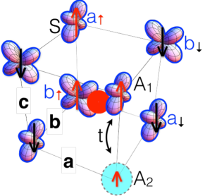
Figure 4: Occupied vanadium $t_{2g}$ orbitals of a V-cube surrounding a Ca defect (red ball) display $G$-type orbital order with alternating $\{a,b\}$ orbitals in all three directions (the occupied $c$ orbitals at the V-ions are not shown). Spins $S=1$ (red/black arrows) reflect $C$-type AF order and the strong Hund’s coupling between $\{a,b\}$ and $c$ electrons at V ions. Due to the kinetic energy ($\propto t$), the doped hole (blue circle) at site $A_{2}$, where the spin $s=1/2$ of the $c$ electron is marked, and the $a$ electron at site $A_{1}$ strongly fluctuate on the FM active bond ($A_{1}$-$A_{2}$) along the $c$ direction.

For the $t_{2g}$ electrons of the vanadium perovskites, the kinetic energy is defined as

$${\cal H}_{{\rm kin}}=-t\sum_{\alpha}\sum_{\left\langle ij\right\rangle\perp\alpha}\sum_{\sigma}\left(d_{i\alpha\sigma}^{\dagger}d_{j\alpha\sigma}+{\rm H.c.}\right),$$ (5)

where we adopt a simplified notation for the $t_{2g}$ orbital basis states Khaliullin and Maekawa (2000):

$$|a\rangle\equiv|yz\rangle,\hskip 14.22636pt|b\rangle\equiv|zx\rangle,\hskip 14.22636pt|c\rangle\equiv|xy\rangle.$$ (6)

The orbital with flavor $\alpha\in\{a,b,c\}$ lies in the plane perpendicular to the cubic crystal axis $\alpha$. In order to fully understand the implications of the actual expression for the kinetic energy (5), one has to take into account that the hopping between two V ions occurs along $\sigma$ bonds via oxygen $p$ orbitals. Due to the spatial symmetry of the V $t_{2g}$ and the O $p$ orbitals, the hopping: (i) conserves the orbital flavor $\alpha$ and (ii) is finite only between $\alpha$ orbitals along bonds $\langle ij\rangle||\gamma$ perpendicular to the direction $\alpha$: $t_{ij}^{\alpha\beta}=t(1-\delta_{\alpha\gamma})\delta_{\alpha\beta}$ and $t>0$. Thus the hopping of $t_{2g}$ electrons is effectively 2D Khaliullin et al. (2001); Harris et al. (2003); Daghofer et al. (2008); Li (2015).

The most relevant Hamiltonian terms to the charge, spin and orbital site occupations are the on-site Hubbard ($U$) and Hund’s exchange ($J_{H}$) interactions (${\cal H}_{{\rm int}}$) for the triply degenerate $t_{2g}$ orbitals Oleś (1983); Daghofer et al. (2010),

$${\cal H}_{{\rm int}} =U\sum_{i\alpha}n_{i\alpha\uparrow}n_{i\alpha\downarrow}-J_{H}\sum_{i}\sum_{\alpha\neq\beta}\mathbf{S}_{i\alpha}\cdot\mathbf{S}_{i\beta}$$

$$+\frac{1}{2}\left(U-\frac{5}{2}J_{H}\right)\sum_{i}\sum_{\alpha\neq\beta}n_{i\alpha}n_{i\beta}$$

$$+J_{H}\sum_{i}\sum_{\alpha\neq\beta}d_{i\alpha\uparrow}^{\dagger}d_{i\alpha\downarrow}^{\dagger}d_{i\beta\downarrow}d_{i\beta\uparrow}.$$ (7)

It is the predominance of the Hubbard and of Hund’s on-site interactions over the kinetic energy that establishes the Mott insulating ground state and the characteristic multiplet structure of states [see top panel of Fig. 1], which is determined by the hierarchy of the charge excitations. The multiplet structure can be considered as the fingerprint of the strong correlations characterizing these systems, and determines ultimately the magnetic properties via the spin-orbital superexchange interactions Oleś et al. (2005).

Finally, there are additional small but nevertheless relevant terms that control the spin-orbital states in these compounds, that is, they determine the anisotropy in the orbital or spin sector, respectively. The last two terms in Eq. (1) reflect small deviations from the cubic symmetry of the cubic vanadates Khaliullin et al. (2001); Horsch et al. (2003); Horsch (2007), where

$${\cal H}_{{\rm CF}}=-\Delta_{c}\sum_{i\sigma}n_{i\sigma c},$$ (8)

is the crystal field that splits the $t_{2g}$ orbitals favoring the $c$ orbital at each site ($\Delta_{c}>0$) Ren et al. (2000). The remaining electron can then occupy either one of the degenerate $a$ and $b$ orbitals. The small Jahn-Teller (JT) interaction acting in the orbital space

$${\cal H}_{{\rm JT}} =\frac{1}{4}V_{ab}\sum_{\langle ij\rangle{\parallel}ab}(n_{ia}-n_{ib})(n_{ja}-n_{jb})$$

$$-\frac{1}{4}V_{c}\sum_{\langle ij\rangle{\parallel}c}(n_{ia}-n_{ib})(n_{ja}-n_{jb}).$$ (9)

favors alternating $\{a,b\}$ orbitals and AO order in the $ab$ plane ($V_{ab}>0$) and the ferro $\{a,b\}$ orbital order along the $c$ crystal axis ($V_{c}>0$) Khaliullin et al. (2001).

So far, the three-band $t_{2g}$ Hamiltonian includes the interactions with charged defects, $e$-$e$ interactions, i.e., short- and long- range, and it provides a faithful description of the magnetic and orbital interactions. The latter is an immediate consequence of the proper description of the atomic multiplet structure. Hence, this model can describe the generic magnetic and orbital ordered phases appearing in the $R$VO₃ perovskites Fujioka et al. (2010), namely two complementary spin-orbital structures: the $C$-AF spin with $G$-AO order and the $G$-type AF spin with $C$-type AO order, as well as a pure AO ordered phase Fujioka et al. (2010).

In the above list of interactions, for the sake of simplicity and clarity of our multiband model, we have omitted certain terms. Among the neglected terms one finds: (i) The relativistic spin-orbit interaction, although small in $3d$ transition metals like vanadium, provides additional orbital fluctuations and contributes to orbital moment formation Horsch et al. (2003, 2008). (ii) The orbital polarization leads to the rotation of orbitals in the proximity of defects and to flavor mixing Horsch and Oleś (2011); Avella et al. (2013). Both terms influence the spin-orbital order and the metal-insulator transition, and would be relevant for a quantitative study of the phase diagram of doped vanadates, which is however not our intention here.

III Hartree-Fock approximation

The main aim of this paper is to analyze the evolution of the spectral weights in the PES and the IPES of strongly correlated spin-orbital system with random charged defects. This is very challenging as it is necessary to treat simultaneously and on equal footing (i) the strong correlation problem (Hubbard) in a multi-orbital system (Hund’s off-diagonal terms and constrained hopping) in presence of strong coupling to the lattice (Jahn-Teller) and of strong fluctuations of all such degrees of freedom, (ii) the local perturbations introduced by the defects into the electronic structure and the long-range nature of their Coulomb potential, which can lead to a potential landscape that can be tuned continuously between monopolar and dipolar, as well as (iii) the randomness of the locations of the defects that necessarily requires a statistical treatment. We demonstrate here that the uHF approach provides an efficient calculation scheme that is able to reproduce the essence of the variations in the spectral weights of the Hubbard bands, provided one deals with a system with broken symmetry as here happens in the spin-orbital sector.

Given the above prescriptions, the derivation of the uHF equations is standard and we do not present it here in extenso; more details can be found, for instance, in Refs. Mizokawa and Fujimori (1995, 1997); Barreteau et al. (2000); Avella et al. (2013). The essence of the derivation is that the $e$-$e$ interactions are replaced by the terms containing mean fields acting on the single-particle electron densities. Following this procedure, one arrives at an effective single-electron Hamiltonian,

$${\cal H}_{{\rm HF}} = \sum_{i\alpha\sigma}\varepsilon_{i\sigma}^{\alpha}n_{i\alpha\sigma}+\sum_{i}\sum_{\alpha\beta\sigma}\gamma_{i\sigma}^{\alpha\beta}d_{i\alpha\sigma}^{\dagger}d_{i\beta\sigma},$$ (10)

$$+ \sum_{ij}\sum_{\alpha\beta\sigma}t_{ij}^{\alpha\beta}d_{i\alpha\sigma}^{\dagger}d_{j\beta\sigma}\,.$$

This Hamiltonian can be diagonalized numerically and the mean fields appearing in the parameters (see below) and the HF states can be determined self-consistently within an iterative procedure. More details on the actual calculation scheme can be found in Appendix A, together with the treatment of the randomness in the present problem.

Following Ref. Avella et al. (2013), we emphasize that Fock terms become active only if their off-diagonal mean fields are finite. This happens only if a single-particle term in the original Hamiltonian (a source for the specific off-diagonal mean fields) induces a finite value for them. Consequently, we adopt here only those Fock terms that couple the same orbitals at neighboring sites (as in the kinetic energy). The terms which couple different orbitals at the same site are inactive in the present study (1) as such terms do not appear in the Hamiltonian Eq. (1) Avella et al. (2013).

Apart from the single-particle tight-binding terms that are treated rigorously, the Hamiltonian (1) includes the JT terms, $e$-$e$ intersite interactions $\propto V_{ij}$, and on-site terms $\propto U$ and $\propto J_{H}$ in Eq. (7). Note that the JT terms in ${\cal H}_{{\rm JT}}$ are effective density-density interactions generated by the JT distortions and, as such, they should be treated in the Hartree approximation. As these and other terms obtained in the Hartree approximation are rather straightforward to evaluate, they will not be listed here and we address below only the Fock terms. The latter terms originate from the $e$-$e$ interactions $\propto V_{ij}$ and contribute effectively to the nearest neighbor hopping terms,

$$-\sum_{\left\langle ij\right\rangle}\sum_{\alpha\sigma}V_{ij}\left\langle d_{i\alpha\sigma}^{\dagger}d_{j\alpha\sigma}\right\rangle\left(d_{i\alpha\sigma}^{\dagger}d_{j\alpha\sigma}+d_{j\alpha\sigma}^{\dagger}d_{i\alpha\sigma}\right).$$ (11)

Formally, such terms appear also for pairs of more distant vanadium ions, but the hopping is limited to nearest neighbors in the model Hamiltonian (1), so they will vanish automatically in the self-consistent solution. Finally, the on-site Coulomb interaction $H_{{\rm int}}$ (7) generates both Hartree and Fock terms, and one finds

$$n_{i\alpha\sigma}n_{i\beta\sigma}\simeq\langle n_{i\alpha\sigma}\rangle\,n_{i\beta\sigma}+n_{i\alpha\sigma}\,\langle n_{i\beta\sigma}\rangle-\langle n_{i\alpha\sigma}\rangle\,\langle n_{i\beta\sigma}\rangle$$

$$-\langle d_{i\alpha\sigma}^{\dagger}d_{i\beta\sigma}\rangle\,d_{i\beta\sigma}^{\dagger}d_{i\alpha\sigma}-d_{i\alpha\sigma}^{\dagger}d_{i\beta\sigma}\,\langle d_{i\beta\sigma}^{\dagger}d_{i\alpha\sigma}\rangle$$

$$+\langle d_{i\alpha\sigma}^{\dagger}d_{i\beta\sigma}\rangle\,\langle d_{i\beta\sigma}^{\dagger}d_{i\alpha\sigma}\rangle,$$ (12)

$$S_{i\alpha}^{+}S_{i\beta}^{-}=d_{i\alpha\uparrow}^{\dagger}d_{i\alpha\downarrow}d_{i\beta\downarrow}^{\dagger}d_{i\beta\uparrow}\simeq$$

$$-\langle d_{i\alpha\uparrow}^{\dagger}d_{i\beta\uparrow}\rangle\,d_{i\beta\downarrow}^{\dagger}d_{i\alpha\downarrow}-d_{i\alpha\uparrow}^{\dagger}d_{i\beta\uparrow}\,\langle d_{i\beta\downarrow}^{\dagger}d_{i\alpha\downarrow}\rangle$$

$$+\langle d_{i\alpha\uparrow}^{\dagger}d_{i\beta\uparrow}\rangle\,\langle d_{i\beta\downarrow}^{\dagger}d_{i\alpha\downarrow}\rangle,$$ (13)

$$d_{i\alpha\uparrow}^{\dagger}d_{i\alpha\downarrow}^{\dagger}d_{i\beta\downarrow}d_{i\beta\uparrow}\simeq\langle d_{i\alpha\uparrow}^{\dagger}d_{i\beta\uparrow}\rangle\,d_{i\alpha\downarrow}^{\dagger}d_{i\beta\downarrow}$$

$$+d_{i\alpha\uparrow}^{\dagger}d_{i\beta\uparrow}\,\langle d_{i\alpha\downarrow}^{\dagger}d_{i\beta\downarrow}\rangle-\langle d_{i\alpha\uparrow}^{\dagger}d_{i\beta\uparrow}\rangle\,\langle d_{i\alpha\downarrow}^{\dagger}d_{i\beta\downarrow}\rangle.$$ (14)

Note however that these latter Fock terms, mixing the orbitals, are included here only to exhaust the approximate treatment of $H_{{\rm int}}$ (7). They would be active, for instance, if the orbitals were optimized locally by a finite orbital polarization interaction Avella et al. (2013), that is not considered here though. Therefore, we do not include them in our analysis as it suffices to decouple the individual terms in Eq. (7) using Hartree approximation.

The uHF calculations in this work are performed for three different sets $\{A,B,C\}$ of fundamental interaction parameters $U$, $J_{H}$ and $V_{D}$ listed in Table 1 for convenience. They have been motivated by different experimental results and/or considerations as parameters relevant for $R$VO₃. Set $A$ is deduced in this work from PES data for the undoped LaVO₃ compound Maiti and Sarma (2000) and gives the positions of the LHB and the UHB multiplet structure in qualitative agreement with the PES and IPES spectra of Maiti and Sarma Maiti and Sarma (2000), see Fig. 2. Set $B$ was deduced from the optical spectroscopy and the magnetic properties of YVO₃ Khaliullin et al. (2004) and was used before to: (i) analyze the magnetic transition from $G$-AF to $C$-AF phase in YVO₃ Horsch and Oleś (2011), and (ii) study the defects in Y_1-xCa_xVO₃ Avella et al. (2013, 2015). Set $C$ is dictated by a simplified analysis of the PES and IPES data in Ref. Maiti et al. (1998), as explained in more detail in Sec. IV.2. Otherwise, we consider $\eta=1$ in Eq. (4) and vary the doping in the range $x\in(0,0.5]$.

Sets $A$ and $C$ are rather similar concerning the most important feature, namely the distance of the centers of LHB and UHB given by $(U-3J_{H})=2.75$ and 3.0 eV, respectively. Set $B$ instead was determined from a model Hamiltonian with only local Hubbard-Hund type interactions, the missing excitonic corrections Mayr and Horsch (2006); Matiks et al. (2009) to the optical gap require in this case a significantly smaller value $(U-3J_{H})=2.2$ eV. An analysis of the parameter $V_{D}$ that defines the defect potential strength as well as the $e$-$e$ interaction will be given in Section VIII. Although our work focuses on the role played by $e$-$e$ interactions, we present in the following calculations both for the realistic set $C$ and for the set $B$, because set $B$ displays features that are somewhat hidden in the spectra calculated using set $C$.

Table 1: The three parameter sets for the interactions in Hamiltonian (1) used in the numerical uHF calculations; all parameters are given in eV. The set $A$ refers to LaVO₃ and was used to obtain the theoretical spectrum in Fig. 2; the remaining sets are for doped systems and include a finite defect potential $V_{{\rm D}}$ (3).

set	$\Delta_{c}$	$U$	$J_{H}$	$V_{ab}$	$V_{c}$	$V_{{\rm D}}$
$A$	0.1	4.1	0.45	0.03	0.05	—
$B$	0.1	4.0	0.6	0.03	0.05	1.0
$C$	0.1	4.5	0.5	0.03	0.05	2.0

IV Doping dependence of the density of states

IV.1 Multiplet structure and sum rules

In this Section, we begin our study of the doped Mott insulator with the DOS $N(\omega)$ of the multiband model in the phase with $C$-type spin and $G$-type orbital order (i.e., $C$-AF/$G$-AO phase). Within the uHF method, $N(\omega)$ describes processes that correspond to the addition of an electron for $\omega>\mu$ and to the removal of an electron for $\omega<\mu$, where $\mu$ is the chemical potential. Thus, $N(\omega)$ provides information relevant for the interpretation of PES and IPES or tunneling experiments Damascelli et al. (2003); Comin and Damascelli (2016). The numerical results presented in this paper are obtained for a cluster of $N_{a}=8\times 8\times 8$ vanadium ions with periodic boundary conditions, after averaging over $M=100$ randomly chosen different Ca defect realizations $\{s\}$ (i.e., sets of randomly chosen Ca defect locations) at a given doping $x\in(0,0.5]$. We use as standard parameters set $B$ of Table 1 and $t=0.2$ eV Khaliullin et al. (2001). For each defect realization $s$, we determine the $6\times N_{a}$ eigenvalues $\{\epsilon_{s,l}\}$ and the value of the Fermi energy $\mu_{s}$. Next, we calculate the final averaged DOS $N(\omega)$, representative for the whole system with $N_{a}$ sites and $xN_{a}$ randomly distributed defects, as an average over the $M$ defect realizations,

$$N\left(\omega\right)\equiv\frac{1}{M}\sum_{s=1}^{M}\left[\frac{1}{N_{a}}\sum_{l=1}^{6N_{a}}\delta(\omega+\mu_{s}-\epsilon_{s,l})\right].$$ (15)

The shapes of the structures arising in the LHB and the UHB are somewhat different in each of the defect realizations $s$, but all of them show the characteristic maxima to be discussed below, see Fig. 5.

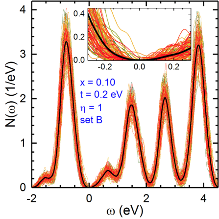
Figure 5: Statistical average of $t_{2g}$ DOS $N(\omega)$ (15) (thick solid black line) as obtained from $M=100$ random defect realizations (thin solid green-to-red lines) for $t=0.2$ eV and including $e$-$e$ interactions ($\eta=1$) at doping concentration $x=0.1$. Other parameters as in set $B$ of Table 1. Inset shows the zoom of the DOS near the Fermi energy at $\omega=0$.

Each charged defect adds a hole to the system, thus the averaging over the different defect realizations is performed for an electron density $n=N_{0}/N_{a}=2-x$ per V ion, and the chemical potential is determined as $\mu_{s}=(\epsilon_{s,N_{0}}+\epsilon_{s,N_{0}+1})/2$. The obtained DOS satisfies the sum rule:

$$\int_{-\infty}^{\infty}d\omega\,N(\omega)=6,$$ (16)

and determines the total number of $t_{2g}$ electrons per site,

$$\int_{-\infty}^{0}d\omega\,N(\omega)=n,$$ (17)

where the overall chemical potential is at $\omega=0$. To control the gradual change of the spectral weights found for the particular structures observed in the DOS, it is convenient to introduce the integrated DOS $n(\omega)$ defined as follows,

$$n(\omega)\equiv\int_{-\infty}^{\omega}d\omega^{\prime}\,N(\omega^{\prime}).$$ (18)

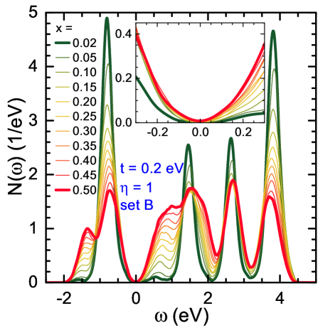
Figure 6: Doping dependence of $t_{2g}$ DOS $N(\omega)$ (15) as obtained from $M=100$ random defect realizations for $t=0.2$ eV and including $e$-$e$ interactions ($\eta=1$) for increasing doping $x\in[0.02,0.50]$. Other parameters as in set $B$ of Table 1. Inset shows the zoom of the DOS near the Fermi energy at $\omega=0$.

Undoped YVO₃ (or LaVO₃) is a Mott insulator and its DOS consists of a LHB and a UHB, separated by a wide MH gap, shown in Fig. 6. The reference here are the data obtained at the lowest value of doping $x=0.02$. The LHB is given by a single maximum with total spectral weight $w_{{\rm LHB}}=2$ in the undoped system, which corresponds to possible one-electron excitations in the PES, see Fig. 2. In contrast, the UHB has three distinct maxima, which reflect the multiplet structure of the excitations accessible in the IPES for the undoped system, as discussed for the two-flavor model in Ref. Horsch and Oleś (2011). We observe that the full width $W$ (at half maximum) of all these structures and of the LHB is $W\simeq 0.5$ eV at low and moderate doping. One could argue that this broadening originates from the incoherence expected for hole (electron) polaron motion in a system with broken symmetry. However, one would expect for a free polaron a width $W_{{\rm inc}}=4\sqrt{z-1}\,t$ Brinkman and Rice (1970), where the number of neighbors for the effective 2D hopping of $t_{2g}$ electrons is $z=4$. This would suggest a much larger value $W_{{\rm inc}}\approx 1.4$ eV. We take this as an indication that the doped holes or polarons are immobile and bound to defects. Hence the broadening is predominantly due to the distribution of the local energies due to the random defect potemtials (see Sec. IV.4). We have shown before that the width of the LHB is $\sim 1.0$ eV in the absence of $e$-$e$ interactions, and is reduced to $\sim 0.5$ eV in the presence of long-range Coulomb interactions Avella et al. (2015), due to the screening of the defect potentials resulting from $t_{2g}$ electrons.

A particularly exciting feature is the persistence of a soft gap right at the chemical potential $\omega=0$ in Fig. 6. Although many defect states fill into the MH gap with increasing doping $x$, it appears that there is a mechanism at work resulting in the highest occupied states and the lowest unoccupied states repelling each other. This is reminiscent of the Peierls effect, but also of the Coulomb gap mechanism. The detailed analysis of the origin of the DS gap in our model is a central issue in this and the following Sections.

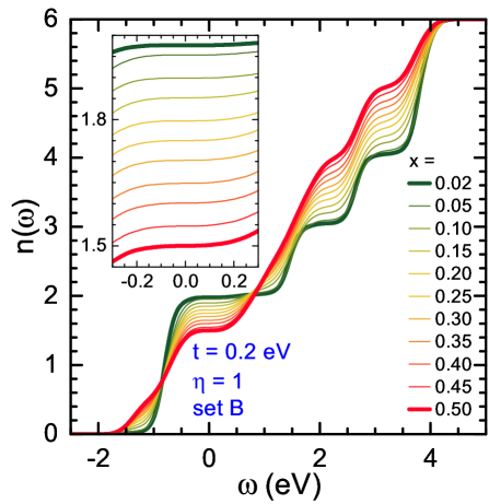
Figure 7: Integrated density of states $n(\omega)$ (18) for different doping concentration $x\in[0.02,0.50]$ obtained for the spectra presented in Fig. 6 for $t=0.2$ eV and including $e$-$e$ interactions ($\eta=1$). Other parameters as in set $B$ of Table 1. Inset shows the zoom of the $n(\omega)$ near the Fermi energy at $\omega=0$.

The DOS obtained for doped $R_{1-x}$Ca_xVO₃ systems preserves the main features seen at $x=0$: the LHB and the UHB are separated by the MH gap, see Fig. 6. With increasing doping $x>0$, the spectral weights below (above) the Fermi energy change in a systematic way. In particular, the fundamental splitting of the MH gap $(U-3J_{H})$ persists up to surprisingly high doping. There arise also new features due to defect states with intensities growing with doping $x$ — one finds a second structure in the LHB at low energy, see Fig. 6. A similar structure with a faster increase of the spectral weight as a function of doping $x$ is observed inside the MH gap at the low-energy edge of the first maximum in the UHB. At the same time, the Hubbard subbands found at $x=0$ persist, but show decreasing spectral intensities with increasing $x$. We analyze these changes in the next Section.

It is insightful to analyze the evolution of the spectra in Fig. 6 by considering the integrated DOS $n(\omega)$ (18). At small doping $x=0.02$, $n(\omega)$ is characterized by several steps that reflect the wide MH gap (wide plateau around $\omega=0$) and the minima of $N(\omega)$ that separate three different states in the UHB (two narrow plateaus), see Fig. 7. With increasing $x$ the plateaus shrink due to the appearance of more and more defect states inside the different gaps. The DOS integrated up to the Fermi energy $\omega=0$ gives the total electron density, $n(0)=n$. That is, the weight of the LHB including the low energy satellite of the LHB is $(2-x)$. A minute increase just above $\omega=0$ indicates that the MH gap is accompanied by a small maximum, arising at finite doping, just above the Fermi energy. For increasing $x$, the maximum above the Fermi energy extends over a broader range, $0.2<\omega<2.0$, suggesting that all structures arising at finite doping are all absorbed within this broader and broader maximum. We turn back to this discussion below in Sec. IV.4.

IV.2 Atomic limit: Exact solution

It is convenient to recall first the main features of the one-particle spectra for the nondegenerate Hubbard model. One of its main successes was to elucidate the variation of the electronic structure in a strongly correlated electronic system with increasing/decreasing electron density and to provide its explanation. It captures the evolution of spectral weights within the individual Hubbard bands Eskes et al. (1991); Meinders et al. (1993); Fujimori et al. (1992); Dagotto et al. (1992); Eskes and Oleś (1994); Eskes et al. (1994); de’Medici et al. (2005). Indeed, in a Mott insulator described by the nondegenerate Hubbard model, the DOS consists of two Hubbard bands, the LHB and the UHB, with equal spectral weights at half filling. These weights however change rather fast in a hole doped insulator when the number of unoccupied states at energies just above the Fermi energy increases — these states belong to the LHB in a system without charged defects Eskes et al. (1991); Meinders et al. (1993); Fujimori et al. (1992); Dagotto et al. (1992). A similar behavior is found for electron doping by applying the particle-hole symmetry. The evolution of spectral weights with increasing doping has been explained within a systematic expansion in $(t/U)$ in the Hubbard model Eskes et al. (1994), but frequently it is sufficient to use only the leading terms of this expansion, which stem from the atomic limit and are written in terms of the electron density. For the nondegenerate Hubbard model at hole doping $x$ this approximation predicts that the LHB has altogether $(1+x)$ states, with $(1-x)$ states below and $2x$ (unoccupied) states above the Fermi energy.

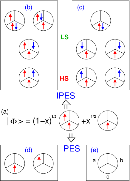
Figure 8: Artist’s view of possible PES (hole doping, bottom) and IPES (electron doping, top) excitations in doped $R_{1-x}$Ca_xVO₃ compounds, as obtained in the HF approximation. In (a), we show a representative ground state $|\Phi\rangle$ with $\uparrow$-spin electron(s) (red arrows) which includes both $|c{\uparrow}a{\uparrow}\rangle$ and $|c{\uparrow}\rangle$ local states in a doped system with amplitudes $\sqrt{1-x}$ and $\sqrt{x}\,$ — we select a V ion on the $\uparrow$-spin sublattice with local undoped (doped) $|c{\uparrow}a{\uparrow}\rangle$ ($|c{\uparrow}\rangle$) state. Adding an electron in IPES (UHB) (blue arrows) generates in this ground state either: (b) four possible $t_{2g}^{3}$ final states with probabilities $(1-x)$ each, or (c) five possible $t_{2g}^{2}$ final states with probabilities $x$ each (with some modifications, see the main text). The states excited in IPES are either HS or LS, with their energies listed in Table 2. Removing an electron (replacing an arrow by a hole) in PES reduces the spin by $1/2$ and gives: (d) either the two $t_{2g}^{1}$ excited states with probabilities $(1-x)$ in the LHB, or (e) an empty $t_{2g}^{0}$ final state with probability $x$. In each panel, three $t_{2g}$ orbitals are labeled as $\{a,b,c\}$ (6), with the convention shown in (e).

In the following, we adopt the atomic perspective and analyze the $C$-AF/$G$-AO states with broken symmetry, addressing also possible deviations resulting from the finite kinetic energy $\propto t$ and from the uHF. For a vanadium perovskite with charged defects the holes added to vanadium ions generate local $t_{2g}^{1}$ configurations with probability $x$, while the $t_{2g}^{2}$ states occur with probability $(1-x)$ in a doped system. This is schematically represented by the ground state wave function $|\Phi\rangle$ for a vanadium ion in Fig. 8(a). In the case depicted in Fig. 8 doping has removed an $|a{\uparrow}\rangle$ electron which has a higher energy than the $|c{\uparrow}\rangle$ electron due to the small crystal field $\Delta_{c}=0.1$ eV, see also Fig. 4. We start from these states to explain the possible PES and IPES excitations, that result from electron removal and addition processes, and lead to final states in the LHB and the UHB, respectively, but also to various defect states.

Table 2: Spectral weights $w_{n}$ and atomic excitation energies $\varepsilon_{n}$ in IPES and PES processes available in doped $R_{1-x}$Ca_xVO₃, leading to final states shown in Fig. 8, as found in the uHF approximation (HF). The energies that involve a doped ion are increased by the energy $V_{{\rm D}}$. The energies found in HF (HF) are compared with those found in the atomic limit (exact) where quantum fluctuations are also included; the spectral weights $w_{n}$ are as in uHF. The HF approach reproduces exact results for PES and for HS IPES states, where only a single energy is shown. For convenience, the PES excitation energy for the host is taken as a reference, $\varepsilon_{{\rm LHB}}=0$ (here, the small crystal-field splitting $\Delta_{c}$ is ignored).

IPES	final state	spin	$w_{n}$	$\varepsilon_{n}$
				HF	exact
$d^{2}\rightarrow d^{3}$	$|c{\uparrow}a{\uparrow}b{\uparrow}\rangle$	HS	$1-x$	$U-3J_{H}$
	$|c{\uparrow}a{\uparrow}b{\downarrow}\rangle$	LS	$1-x$	$U-J_{H}$	$U$
	$|c{\uparrow}a{\uparrow}c{\downarrow}\rangle$	LS	$1-x$	$U+J_{H}$	$U$
	$|c{\uparrow}a{\uparrow}a{\downarrow}\rangle$	LS	$1-x$	$U+J_{H}$	$U+2J_{H}$
$d^{1}\rightarrow d^{2}$	$|c{\uparrow}a{\uparrow}\rangle$	HS	$x$	$V_{{\rm D}}$
	$|c{\uparrow}b{\uparrow}\rangle$	HS	$x$	$V_{{\rm D}}$
	$|c{\uparrow}b{\downarrow}\rangle$	LS	$x$	$V_{{\rm D}}+J_{H}$	$V_{{\rm D}}+2J_{H}$
	$|c{\uparrow}a{\downarrow}\rangle$	LS	$x$	$V_{{\rm D}}+J_{H}$	$V_{{\rm D}}+2J_{H}$
	$|c{\uparrow}c{\downarrow}\rangle$	LS	$x$	$V_{{\rm D}}+3J_{H}$	$V_{{\rm D}}+5J_{H}$
PES	final state	$-$	$w_{n}$	$\varepsilon_{n}$
$d^{2}\rightarrow d^{1}$	$|c{\uparrow}\rangle$	$-$	$1-x$	$0$
	$|a{\uparrow}\rangle$	$-$	$1-x$	$0$
$d^{1}\rightarrow d^{0}$	$|0\rangle$	$-$	$x$	$V_{{\rm D}}-(U-3J_{H}$)

In IPES, one electron is added in the $d^{n}\rightarrow d^{n+1}$ process, either to the $|c{\uparrow}a{\uparrow}\rangle$ initial configuration ($n=2$), see Fig. 8(b), or at a V ion with a hole in the $|c{\uparrow}\rangle$ initial state ($n=1$), see Fig. 8(c). As the doped sites are typically direct neighbors of a charge defect, the electron energies at these sites are increased by $V_{{\rm D}}$ (3). Thus the HS states generated by $d^{1}\rightarrow d^{2}$ IPES transitions appear as in-gap states above the Fermi energy. But there is also a multiplet structure of the $d^{2}$ final states that overlaps partially with the $t_{2g}^{3}$ multiplet states of the UHB as can be infered from Fig. 8. Altogether, the IPES excited states are quite numerous, four and five for the two cases listed above, and their spin is either increased by 1/2 in HS states, or decreased by 1/2 in LS excited states. Their exact energies are given in Table 2.

Taking all the states generated in IPES one finds their total weight of $(4+x)$ which is a generalization of the $(1+x)$ found in the nondegenerate Hubbard model Meinders et al. (1993) and the $(3+x)$ for the two-flavor model in Ref. Horsch and Oleś (2011). The UHB obtained for $d^{2}\rightarrow d^{3}$ excitations has three subbands corresponding to the atomic multiplet structure with energies $(U-3J_{H})$, $U$, and $(U+2J_{H})$ as given in Table II. They are found from the exact solution treating rigorously the Coulomb interactions for $t_{2g}^{3}$ excited states in the atomic limit. In a doped system, the initial $t_{2g}^{2}$ state occurs in the wave function $|\Phi\rangle$ with the probability $(1-x)$, see Fig. 8(a). Therefore, the weights of these excitations are: $(1-x)$, $2(1-x)$, and $(1-x)$. This weight distribution is modified when quantum fluctuations are neglected, see below.

Let us compare first the results obtained for the PES and IPES spectra with the experimental results for undoped LaVO₃ shown in Fig. 2. The spectrum consists of two distinct structures, the LHB and the UHB separated by a broad MH gap. From the experimental spectra one learns that the distance that separates the LHB and the HS excitation in the UHB is $3.0$ eV. This gives the first experimental constraint on the on-site Coulomb interaction parameters $\{U,J_{H}\}$ — this energy difference obtained in the theory is $(U-3J_{H})$, see Table 2. Furthermore, for the undoped LaVO₃, the HF theory predicts three peaks in the UHB, with the HF energies of $(U-3J_{H})$, $(U-J_{H})$, and $(U+J_{H})$ for the HS, LS₁, and LS₂ excitations, see Table II. The energetic separation of the LS₂ and the HS states is thus $4J_{H}$ that determines the lower bound for the width of the UHB, to be still enhanced by the experimental broadening. Note that the same result would be obtained in the electronic structure calculations implementing the leading part of local Coulomb interactions Vaugier et al. (2012).

As explained above, the highest excitation energy for the LS₂ states is doubly degenerate in HF which gives here twice larger spectral weight than that of the other two excitations, HS and LS₁. In contrast, the LS₁ state is doubly degenerate when quantum effects are included (see Table 2) and the correct weights’ distribution is 1:2:1 for the HS, LS₁, and LS₂ states. In Fig. 2, we have adjusted the spectral weights of the uHF spectra accordingly to achieve a better agreement with experiment. Unfortunately, the individual excitations within the UHB cannot be resolved in the data Maiti and Sarma (2000). The whole spectrum formed by the LHB and UHB are reproduced well by the theory, see Fig. 2, after adjusting the two characteristic parameters $\{U,J_{H}\}$ that define the position of the maximum seen in the UHB at the energy $(U-J_{H})$ of the LS₁ state, i.e., relative to the energy of the LHB. The best fit was obtained with $U=4.1$ eV and $J_{H}=0.45$ eV that defines the set $A$ of Table 1. Apart from a somewhat decreasing overall experimental spectral weight with increasing excitation energy $\omega$, which cannot be reproduced without additional information about the matrix elements, the agreement between the experiment and the theory predictions is indeed very satisfactory and demonstrates the presence of a multiplet structure within the UHB.

The analysis of the IPES excitations summarized in Table 2 elucidates additional features generated in the spectra by doping. For the $|c{\uparrow}\rangle$ component of the ground state wave function $|\Phi\rangle$ [Fig. 8(a)], with a hole in the initially occupied $a$ orbital, two HS states and three LS states may be generated by IPES, see Fig. 8(c). Each of these states will have a spectral weight $x$. In contrast to the excitations occurring in the host shown in Fig. 8(b), the HS excitations at a doped site include two final $t_{2g}^{2}$ states, either $|c{\uparrow}a{\uparrow}\rangle$ or $|c{\uparrow}b{\uparrow}\rangle$, with the same local Coulomb energy $(U-3J_{H})$ as for $t_{2g}^{2}$ host states. Thus, these excitation energies $\varepsilon_{n}$ do not include the intraatomic Coulomb $U$ or exchange $J_{H}$ and would appear just above the LHB in the absence of a defect potential (i.e., at $V_{{\rm D}}=0$) Meinders et al. (1993). However, in reality the $d^{1}\rightarrow d^{2}$ excitation energy is enhanced by large $V_{{\rm D}}$ near the charged impurity in the center of the cube occupied by the defect (Fig. 4) and these unoccupied states appear deep within the MH gap. The defect potential $V_{{\rm D}}$ acts on any local state and enhances its excitation energy, see Table 2. The two LS states with two different orbitals singly occupied have the final energies of $(U-J_{H})$, so the excitation energies are $2J_{H}$. The excitation involving double occupancy $|c{\uparrow}c{\downarrow}\rangle$ is more subtle: This state itself is not an eigenstate of $H_{\rm int}$ (7) as a double occupancy couples by the term $\propto J_{H}$ to $|a{\uparrow}a{\downarrow}\rangle$ or $|b{\uparrow}b{\downarrow}\rangle$ state. As a result, the highest excitation energy $(V_{{\rm D}}+5J_{H})$ is obtained only for one (fully symmetric with respect to orbital permutations) eigenstate while the energy $(V_{{\rm D}}+2J_{H})$ for the other two. Eventually, the configuration $|c{\uparrow}c{\downarrow}\rangle$ shown in Fig. 8(c) is found with the probability of $1/3$ in each of these eigenstates. Hence, by performing the corresponding projections, one finds that the final exact atomic spectral weights for the energies $(V_{{\rm D}}+2J_{H})$ and $(V_{{\rm D}}+5J_{H})$ are $8x/3$ and $x/3$.

Here again quantum fluctuations contribute and the HF energies of two interorbital LS states, $|c{\uparrow}a{\downarrow}\rangle$ and $|c{\uparrow}b{\downarrow}\rangle$, are lower by $J_{H}$, i.e., by the same amount as found for the final LS states in the case of $d^{2}\rightarrow d^{3}$ excitations. The other states are given by the double occupancies that are here eigenstates at energy $U$, so the excitation energy for the accessible $|c{\uparrow}c{\downarrow}\rangle$ state is $(V_{{\rm D}}+3J_{H})$, see Table II. The HF spectral weights for the LS₁ and LS₂ states are thus $2x$ and $x$.

The PES excitations are much simpler than the IPES ones as just one electron is removed from either component of the ground state wave function shown in Fig. 8(a) and the spin is then reduced by $1/2$. The $d^{2}\rightarrow d^{1}$ excitations in the host have approximately the same excitation energy taken here as the reference, $\varepsilon_{n}=\varepsilon_{{\rm LHB}}=0$ (we neglect again the crystal-field term $\propto\Delta_{c}$). In contrast, a PES excitation at the hole site, $d^{1}\rightarrow d^{0}$, starts from the $|c{\uparrow}\rangle$ state, so the energy of the $d^{2}$ reference configuration is subtracted from $V_{{\rm D}}$ in Table 2.

IV.3 Spectral weight distribution in the atomic limit

To illustrate the above theory, we determined the individual structures in PES/IPES spectra and their evolution with increasing doping $x\in[0.02,0.50]$ for $t=0.01$ eV. Here, the kinetic energy is chosen to be very small indeed to generate the results representative for the atomic limit. In Fig. 9, one observes that the MH gap persists in doped systems. The LHB is well separated from the HS excitation in the UHB by the MH gap for the entire doping regime. The states arising within the MH gap do not close this gap but develop a novel kinetic gap analyzed in more detail in the next Sec. V.

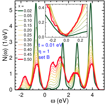
Figure 9: Doping dependence of $t_{2g}$ DOS $N(\omega)$ (15) as obtained from $M=100$ random defect realizations for $t=0.01$ eV and including $e$-$e$ interactions ($\eta=1$) for increasing doping $x\in[0.02,0.50]$. Other parameters as in set $B$ in Table 1. Inset shows the zoom of the DOS near the Fermi energy at $\omega=0$.

PES excitations (at $\omega<0$) are seen in the spectra as two structures: (i) the LHB corresponding to individual $d^{2}\rightarrow d^{1}$ transitions at V sites that are not nearest neighbors of defects; (ii) a satellite below the LHB at energy $\sim-2.0$ eV, i.e., originating from $d^{1}\rightarrow d^{0}$ processes at sites occupied by doped holes, see Fig. 9. When the doping $x$ increases, the spectral weight of the PES part is altogether $\sim(2-x)$, which consists of the main peak representing the LHB $\sim(2-2x)$ and a satellite generated by the excitations at the hole sites with growing spectral weight $\sim x$. This agrees with the spectral weights of the PES states listed in Table II. The satellite moves gradually towards the LHB, reaching energy $\sim-1.7$ eV at $x=0.45$. Excitations from undoped sites near defects are close to the Fermi energy and can be well resolved from the main maximum in the LHB.

The three multiplet transitions $d^{2}\rightarrow d^{3}$ that appear in the IPES part of the uHF spectra are surprisingly well resolved even at high doping. The spectral weights of these UHB states of the host compound are $(1-x)$, $(1-x)$, and $2(1-x)$ for the HS, LS₁ and LS₂ states, see Fig. 9. The defect related features in the IPES part ($\omega>0$) due to $d^{1}\rightarrow d^{2}$ excitations are better resolved here than in case of $t=0.2$ eV (Fig. 6). There are two distinct peaks that grow with doping within the MH gap, at energies $\sim 0.6$ eV and $\sim 1.2$ eV. While the weight of the lower maximum accumulates the weight $\sim 2x$, the weight if the second maximum appears even somewhat larger. We recall that the weight of the satellite below the LHB is $\sim x$, see Table II. The third maximum induced by doping falls near the minimum separating the HS from the LS₁ excitation in the reference multiplet structure of the UHB (for these parameters) and has a lower weight $\sim x$. In addition, a spectacular evolution of pseudogap in $N(\omega)$ close to $\omega=0$ is found (see inset). The highly asymmetric spectrum changes gradually to an almost symmetric one with increasing $x$.

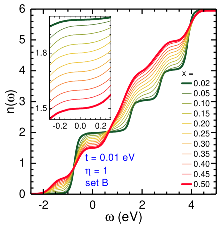
Figure 10: Integrated density of states $n(\omega)$ (18) for different doping $x\in[0.02,0.50]$ obtained for the spectra presented in Fig. 9 at $t=0.01$ eV and including $e$-$e$ interactions ($\eta=1$). Other parameters as in set $B$ in Table 1. Inset shows the zoom of the $n(\omega)$ near the Fermi energy at $\omega=0$.

The modifications of the DOS $N(\omega)$ with increasing doping $x$ shown in Fig. 9 can be even better appreciated by analyzing the integrated DOS, see Fig. 10. First of all, one finds an almost flat plateau in the integrated DOS at $n(\omega)\simeq 1.98$ at low doping $x=0.02$, and the plateau at $\omega=0$ persists at higher doping. At $x=0.02$, large steps of $(1-x)$ are found for the energies of the HS and LS₁ states in the UHB, and of $2(1-x)$ at energy of the LS₂ state. Note that this latter excitation is well separated from the structures generated by excitations at sites doped by holes as the former energies are lower. Most importantly, the excitation energies are constant and are not influenced by increasing doping, reflecting the robust local character of both $d^{2}\rightarrow d^{3}$ and $d^{1}\rightarrow d^{2}$ processes.

At the lowest doping $x=0.02$, one is sufficiently close to the reference undoped system characterized by the LHB at $\omega\sim-0.8$ eV, and the weak satellite feature with low intensity arises at $\omega\simeq-2.0$ eV, identified by finite $n(\omega)$ for $-2.0<\omega<-1.0$ eV. By removing a single electron one gains here the energy $V_{{\rm D}}$ as this electron before the removal feels the potential of the charged defect $V_{{\rm D}}$ in the center of the cube, see Table II. Indeed, this latter excitation energy is lower than that at the center of the LHB, as observed in Fig. 9. Faster increase of $n\left(\omega\right)$ follows close to $\omega=-0.8$ eV and afterwards the integrated weight grows again very slowly. Finally, the spectral features that grow with increasing doping in Fig. 9 are responsible for the dramatic deformation of a distinct step structure seen in Fig. 10 at $x=0.02$ towards an almost steady increase of $n(\omega)$ from the onset of the LHB to the top of the UHB, except for a quite narrow plateau near the Fermi energy shown in the inset.

We also observe a remarkable feature in Fig. 10: Independently of actual doping $x$, the integrated DOS reaches the value of two electrons per site at $\omega\simeq 0.7$ eV. This shows that the spectral weight missing in the PES part is compensated by the HS $d^{1}\rightarrow d^{2}$ excitations which have an approximately constant energy above the Fermi level in the entire doping regime. A similar point is found at $\omega\simeq-0.8$ eV and the filling of $n(\omega)=0.8$ — here it falls around the maximum of the LHB. These points are quite reminiscent of the isosbestic point found in the specific heat of correlated systems Vollhardt (1997); Greger et al. (2013). Here the two isosbestic points originate from the doping dependent spectral weight tranfers between the host Hubbard bands and the defect states, that correspond to the final states of the $d^{1}\rightarrow d^{0}$ and $d^{1}\rightarrow d^{2}$ transitions, respectively.

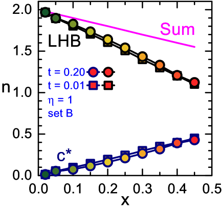
Figure 11: Doping dependence of the total spectral weight below the Fermi energy (Sum, magenta line), of the LHB (LHB, black symbols) originating from undoped V sites and from the satellite arising due to PES excitations at V doped ions $|c_{i\sigma}^{*}|0\rangle$ ($c^{*}$, blue symbols) bound by a charged defect, as obtained near the atomic limit for $t=0.01$ eV (squares) and at the value $t=0.2$ eV realistic for Y_1-xCa_xVO₃ (circles). Other parameters as in set $B$ in Table 1.

Summarizing, by analyzing the data in Figs. 6 and 9, one concludes that the spectral weights found in the numerical calculations both confirm those found in the atomic limit, see Table 2. The total spectral weight of the occupied part of the DOS, $2-x$, reproduces the average electron density below the Fermi energy. This weight consists of that of the LHB, represented by the main peak in the spectra, which corresponds to $d^{2}\rightarrow d^{1}$ transitions at undoped sites with the total intensity $2(1-x)$, and that of the satellite growing at low energy with the weight of $x$ as it reflects the $d^{1}\rightarrow d^{0}$ excitations at the V ions with doped holes in bound states near the defects. The predicted linear behavior $\propto x$ is indeed reproduced at $t=0.01$ eV, see Fig. 11, while only a small deviation from it is observed for $t=0.2$ eV. One finds that the spectral weight in the LHB is somewhat enhanced at the expense of the $d^{1}\rightarrow d^{0}$ satellite. This behavior is reminiscent of the kinetic spectral weight transfer in the nondegenerate Hubbard model Eskes et al. (1991); Meinders et al. (1993).

IV.4 Active bond and satellite of the LHB

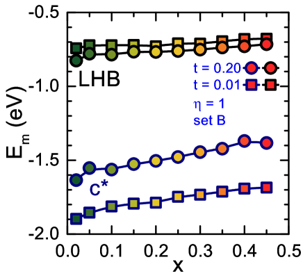
Figure 12: Excitation energies $E_{m}$ assigned to the LHB $d^{2}\rightarrow d^{1}$ and the satellite $c^{*}$ attributed to $d^{1}\rightarrow d^{0}$ excitations arising from hole-like small polarons, where the doped holes (or $d^{1}$ configurations) are localized at V-ions close to a charged Ca defect. Data for $R_{1-x}$Ca_xVO₃ is shown for $t=0.2$ eV (circles) and for the atomic limit $t=0.01$ eV (squares). Other parameters as in set $B$ of Table 1.

We emphasize that the satellite structure arising from the $d^{1}\rightarrow d^{0}$ excitation is well separated from the remaining states in the LHB only in a particular range of parameters and in addition when the hopping is small, $t=0.01$ eV. For such an immobile hole the excitation energy is practically the same as in the atomic limit, see Table 2,

$$E_{m}^{(0)}=E_{{\rm LHB}}+V_{{\rm D}}-(U-3J_{H}).$$ (19)

Thus, to get the excitation energies in the case of $t=0.01$ eV one has to include the energy corresponding to the center of the LHB, being $E_{{\rm LHB}}=-0.7$ eV in Fig. 12, and combine it with the energy of the $d^{1}\rightarrow d^{0}$ excitation $(V_{{\rm D}}-U+3J_{H})$, and one arrives at the excitation energy $E_{m}^{(0)}=-1.9$ eV shown in Fig. 12 for the low doping $x=0.02$.

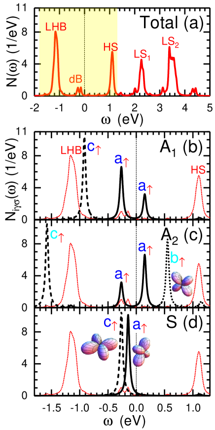
Figure 13: Single particle excitations: (a) Multiplet structure (Total) in the presence of well annealed, or equivalently short-range-potential random, charged defects, in yellow the energy region reported in the other panels; (b-c) Partial spectral weights $N_{i\gamma\sigma}(\omega)$ for vanadium ions $A_{1}$ and $A_{2}$, respectively, that belong to the active bond, and (d) for an occupied spectator site $S$ as defined in Fig. 4. The hole is predominantly at $A_{2}$. In (b-d), the thin dashed red curves represent the total DOS (from panel a) and is given as reference. Parameters as in set $B$ of Table 1 and $t=0.2$ eV.

Consider now a doped site $i$ at finite and increasing $t$. The hole as well as the other occupied V neighbors closest to a given Ca²⁺ defect (on a cube $\mathcal{C}_{m}$ surrounding a defect at site $m$) feel the potential $V_{{\rm D}}$ Avella et al. (2013). The hole delocalizes partly along the active FM bond $\langle ij\rangle{\parallel}c$ axis, and electronic configurations at sites $i$ and $j$ change from $(b{\uparrow})^{0}$ and $(b{\uparrow})^{1}$ to $(b{\uparrow})^{\delta}$ and $(b{\uparrow})^{1-\delta}$ (with $\delta<0.5$ and $(c{\uparrow})^{1}$ electron at each site). This results in the modification of excitation energies at both sites and one finds instead of Eq. (19):

$$E_{m}^{(i)} = E_{{\rm LHB}}+V_{{\rm D}}-(U-3J_{H})\,(1-\delta),$$ (20)

$$E_{m}^{(j)} = E_{{\rm LHB}}+V_{{\rm D}}-(U-3J_{H})\,\delta.$$ (21)

This is illustrated through a calculation for well annealed, or equivalently short-range-potential random, charged defects shown in Fig. 13. In this figure, together with the reference overall multiplet structure (panel a), the partial DOS $N_{i\gamma\sigma}(\omega)$ at three V sites of the defect cube (see Fig. 4) are displayed. Namely, sites $A_{1}$ (panel b) and $A_{2}$ (panel c) that belong to the FM active bond that basically accommodates the doped hole, and, for comparison, at a site with two electrons which we call a spectator ($S$) site, see Fig. 4(d). In the latter case, both electrons $a$ and $c$ feel the Hubbard interaction $(U-3J_{H})$. The remaining single $a$ electron on the active bond forms a bonding state, whose polarity is determined by several factors: (i) the interplay of kinetic energy and JT-fields and (ii) in the long-range-potential case with random defects, the random fields of the other defects. Even in absence of random defect potentials a hole distribution polarized along the $c$ axis is expected, favored by the JT potentials in the symmetry broken $G$-AO state.

The energies of the occupied $c$ levels at sites $A_{1}$ and $A_{2}$ in Fig. 13 are very different, as they are controlled by the distribution of the single $a$-electron on the active bond $\langle A_{1},A_{2}\rangle$. In Fig. 13, the hole is mainly at site $A_{2}$ and, therefore, the $c$ electron there is at a lower energy as it does not acquire the Hubbard interaction $(U-3J_{H})$ due to the smaller density of $a$-electrons at site $A_{2}$. The position of the satellite $c^{*}$ coincides with the occupied $c$-level at site $A_{2}$ and therefore monitors the polarity of the active bond and, in the disordered case, the random fields of the further distant defects.

Hole delocalization on the active bond with increasing $t$ reduces the energetic distance between the LHB and the satellite state $c^{*}$, see Fig. 12. As we have explained above, see Eq. (20), this $\delta$-dependent energy shift by $[V_{{\rm D}}-(U-3J_{H})(1-\delta)]$ is a fraction of the Coulomb energy $(U-3J_{H})$ and is therefore much higher than $t$ itself. In the considered example in Fig. 12, one finds the value $E_{m}^{(1)}\simeq-1.6$ eV for $t=0.2$ eV which implies a hole delocalization on the active bond corresponding to $\delta\approx 0.3$. Thus the distance of the $c^{*}$-excitation can be used to probe the delocalization of the doped hole on the active bond. As the delocalization is controlled by the interplay of the kinetic matrix element $t$ and the random defect fields, the $d^{1}\rightarrow d^{0}$ excitation energies provide a direct measure of the strength and the fluctuations of the random fields.

So far we have focused on the multiplet structure and on the $d^{1}$ defect state that gives rise to a satellite on the low energy side of the LHB, and should appear as $d^{1}\rightarrow d^{0}$ transition in PES. The observation of the satellite would yield valuable information about the defect structure and the disorder strength. In the next Section, we turn to further defect related transitions, namely the $d^{2}\rightarrow d^{1}$ transitions in PES and $d^{1}\rightarrow d^{2}$ transitions in IPES. The corresponding electron removal and addition energies fall inside the fundamental MH gap and lie below and above the chemical potential, respectively.

V Mechanisms for defect states gap

The most important features triggered by the presence of charged defects in the system are the (defect) states that appear within the MH gap as they determine the position of the chemical potential and the transport properties of the material. Such states originate from the LHB and, being repelled by effectively negative defects (for instance, Ca²⁺ ions substituting La³⁺ ones), are pushed upwards in energy into the MH gap. The distribution $N_{0}(\omega)$ of the bare electron energies $h_{i}$, as defined in Eq. (2), is determined by the Coulomb potentials of the random Ca²⁺ impurities. An example is shown for doping $x=10$% in Fig. 14(a). The total distribution of electron energies $N_{0}(\omega)$ [see Fig. 14(a)] can be decomposed into the distribution $N_{d}(\omega)$ of energies of the V sites that are direct neighbors of at least one defect, i.e., within distance $d$, while the remaining V sites contribute to the second distribution $N_{nd}(\omega)$ that lies at lower energy, as shown in Figs. 14(c-d), respectively.

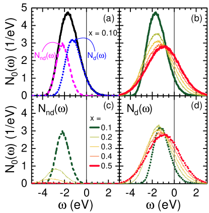
Figure 14: Distribution of the local energies $h_{i}$ due to the random defect potentials. (a) The total distribution of levels $N_{0}(\omega)$ (solid black line) for a doping concentration $x=10$% is subdivided in a distribution $N_{d}(\omega)$ of energy levels of V sites that are direct neighbor of at least one defect (dotted blue line) and a remaining distribution $N_{nd}(\omega)$ of levels related to V sites that are not nearest neighbor of a defect (dashed magenta line). (b) $N_{0}(\omega)$ , (c) $N_{nd}(\omega)$ and (d) $N_{d}(\omega)$ for doping concentrations $x$ from 10% to 50% (green to red lines). The chemical potential $\mu$ (corresponding to $\omega=0$) lies in the high energy tail of the level distribution $N_{d}(\omega)$ related to V sites that are nearest neighbor of a defect.

Figure 14 highlights three important points: (i) as there are 8 vanadium sites close to each defect, but only a single hole per defect, the number of defect states is much larger than the number of doped holes; (ii) hence, the chemical potential $\mu$ lies in the high energy tail of the defect state distribution $N_{d}(\omega)$ [see Fig. 14(d)]; (iii) the defect states distribution below $\mu$ is not well separated from the states of the original LHB. The latter point, namely that the defect states in the Hubbard gap below $\mu$ and the LHB states cannot be easily distinguished, is a common feature of $N_{0}(\omega)$ and of the total DOS $N(\omega)$ of the system studied in the previous Section (see Fig. 6). On the contrary, above $\mu$, that is in the IPES regime, the defect states and the HS Hubbard band states appear well separated in energy.

The opening of a soft DS gap at the chemical potential $\mu$ in $N(\omega)$ is the most striking difference with respect to the bare DOS $N_{0}(\omega)$. Figure 6 displays the pronounced depletion of the DOS $N(\omega)$ right at the chemical potential (i.e., within the defect states band) for a system with long-range $e$-$e$ interactions ($\eta=1$) and several doping concentrations. One well-known mechanism for the opening of a soft gap is the combined action of long range $e$-$e$ interactions and disorder as pioneered by Pollak Pollack (1970) and by Efros and Sklovskii Efros and Shklovskii (1975); Efros (1976) and denoted as the Coulomb gap Efros and Shklovskii (1975). The Coulomb gap arises from a subtle optimization of the occupation of randomly distributed localized electron states, viz. the CG model, where the total energy is minimized by the formation of a soft gap around the chemical potential.

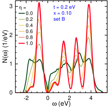
Figure 15: Variation of the density of states and of the defect states gap for parameter set $B$ of Table 1 as function of the strength of $e$-$e$ interactions $\eta=0,0.2,0.4,0.6,0.8,1.0$ and $t=0.2$ eV.

An alternative mechanism for the formation of a gap in cubic oxides in the presence of charged defects was reported in a recent study Avella et al. (2013, 2015). In these systems, the gap arises because the doped holes: (i) are bound to the defects by the defect potential whereas the spin-orbital order greatly reduces the already constrained (2D) mobility; (ii) are confined to one of the vertical bonds of the defect cube hosting them by the in-plane AF spin order; (iii) can gain kinetic energy, leading to a splitting of the topmost occupied states, delocalizing over that vertical bond. That is, the system gains energy by opening a gap at the chemical potential as in the Peierls effect. However, here the splitting does not arise from an induced lattice distortion, but from the formation of bonding and anti-bonding states on the FM active bond $\langle A_{1},A_{2}\rangle$ close to a defect in the presence of a doped hole, as it is depicted in Fig. 13. The formation of a kinetic gap between the $|a{\uparrow}\rangle$ states in Fig. 13 is controlled by an interplay of doped holes with spin and orbital degrees of freedom, and most importantly it is controlled by the random potentials of the defects and the $e$-$e$ interaction. Furthermore, it was found that the kinetic gap is not destroyed by disorder if $t$ is large enough Avella et al. (2015).

For a general case, it was pointed out that the kinetic and the Coulomb gap mechanisms, the latter emerging from $e$-$e$ interactions, enhance jointly the DS gap in the vanadates Avella et al. (2013). We note that this is in contrast to the Anderson-Hubbard model with long-range $e$-$e$ interactions where the kinetic energy suppresses the DS gap Epperlein et al. (1997).

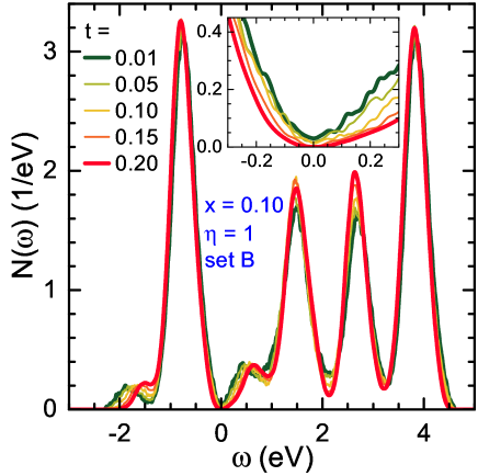
Figure 16: Variation of the density of states and of the defect states gap for parameter set $B$ of Table 1 for $t=0.01,0.05,0.10,0.15$, and $0.20$ eV, and $\eta=1$. Inset shows the zoom of the DOS near the Fermi energy at $\omega=0$.

Here, we present a systematic analysis of how the $e$-$e$ interactions and the kinetic-gap mechanism jointly contribute to the formation of the DS gap. In Fig. 15, for a system with doping $x=10$%, we investigate how the DOS $N(\omega)$ varies when the $e$-$e$ interaction is switched on while keeping the value of the hopping integral $t=0.2$ eV fixed. This is done by changing the $\eta$ parameter from zero to one; notice that this corresponds to the line BC in Fig. 1. At $\eta=0$, the quite large width of the Hubbard bands is due to the effective distribution of the levels generated by the Coulomb potentials of the random defects (see Fig. 14). With increasing $\eta$, such monopolar potentials ($\propto 1/r$) are more and more compensated by the $e$-$e$-interaction. In the case $\eta=1$, i.e., in the physical case, each single defect and the related bound hole act overall as a dipole ($\propto 1/r^{2}$) and, as a consequence, the effective distribution of the random energy levels gets narrower while keeping the defect positions unchanged. In Fig. 15, there is already a kinetic gap even in the complete absence of $e$-$e$ interactions ($\eta=0$). This gap is approximately linear in $\omega$ as we shall see in the statistical analysis below. With increasing $\eta$, a pronounced soft gap evolves, that can be attributed to the Coulomb gap mechanism.

In Fig. 16, we study the $t$ dependence at $\eta=1$, i.e., in presence of $e$-$e$ interactions, for doping $x=10$%. This corresponds to the line DC in Fig. 1. The DOS changes only slightly as a function of $t$ as the width of the Hubbard bands is essentially determined by the disorder. The evolution of the DS gap is amplified in the inset of Fig. 16. Surprisingly, we see here that, at small values of $t$, the Coulomb gap mechanism in these systems is not strong enough to create a soft gap. In a certain range $t\leq t^{*}$, the data in the inset suggests that the DOS at $\mu$ is finite. As there is nevertheless a strong suppression of the DOS we call this a pseudogap. With increasing $t$, the pseudogap changes into a soft gap with $N(\mu)=0$. We shall see below by a rigorous statistical analysis that for small $t$ values there is in fact a weak singularity with $N(0)=0$ hidden in this data. As a side remark, we note that, with increasing $t$, the satellite $c^{*}$ gradually moves upward. The upward shift is connected with the increasing delocalization of the hole on the active bond, as discussed above.

To analyze the behavior of the soft gap in $N(\omega)$ without suffering from the unavoidable broadening of delta functions, we consider the averaged integrated DOS $n(\omega)$ Eq. (18) that can be studied without artificial broadening. It is worth noting the following key features of $n(\omega)$ in the vicinity of the Fermi energy: (i) at the chemical potential there is an evident gap/plateau for $t=0.2$ eV and $\eta=1$ [see Fig. 7], but not for $t=0.01$ eV, and (ii) on decreasing the screening $\eta\rightarrow 0$, the gap/plateau disappears even for $t=0.2$ eV.

In order to establish the statistical behavior of $N\left(\omega\right)$ at low energy in the limit of an infinite number of defect realizations $M\to\infty$, we use that $N\left(\omega\right)$ is proportional to the probability distribution function $P^{*}\left(\omega\right)$ that the topmost occupied state (the lowest unoccupied state) in a generic defect realization $s$ has energy $\omega=\Delta_{s}\left(-\Delta_{s}\right)$ relative to its Fermi energy $\mu_{s}$. This is equivalent to the distribution of the nearest neighbor level spacings $2\Delta_{s}$ across the chemical potential. In Ref. Avella et al. (2015), it has been shown that a generic defect realization features a gap of size $E$ with a probability governed by a Weibull probability distribution function,

$$P_{W}(E)=\theta\!\left(E-\zeta\right)\,\frac{k}{\lambda}\,\left(\frac{E-\zeta}{\lambda}\right)^{k-1}\mathrm{e}^{-\left(\frac{E-\zeta}{\lambda}\right)^{k}},$$ (22)

with shape parameter $k$, scale parameter $\lambda$ and location parameter $\zeta$. Accordingly, if $\zeta=0,$ we have $P^{*}\left(\omega\right)=\frac{k}{\lambda^{k}}\left|\omega\right|^{k-1}$ and $N\left(\omega\right)\propto\left|\omega\right|^{k-1}$ both for $\left|\omega\right|\ll\lambda$. The exponent $k$ allows to distinguish the following cases: a soft gap for $k>2$, a linear gap for $k=2$, a pseudogap (or singular gap) regime for $1<k<2$ and no gap for $k=1$.

Moreover, if $\zeta>0$ the Weibull probability distribution describes a real gap, that is in this case we have $N\left(\omega\right)=0$ for $\left|\omega\right|\leq\zeta$ and $N\left(\omega\right)\propto\left(\left|\omega\right|-\zeta\right)^{k-1}$ for $\zeta<\left|\omega\right|\ll\lambda$. Thus, $P_{W}\left(E\right)$ results in a robust scheme to determine the behavior of $N\left(\omega\right)$ close to the Fermi energy, that is, the presence and type of the overall gap in the system (through $k$ and $\zeta$) as well as the typical scale of the microscopic gap developing locally in the system because of all microscopic mechanisms at work (through $\lambda$).

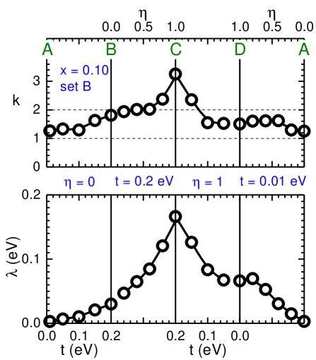
Figure 17: Shape $k$ (top) and scale $\lambda$ (bottom) parameters of the Weibull distribution (22) that characterizes the soft gap at $\mu$ as function of $e$-$e$-interaction strength $\eta$ for $t=0.2$ eV (BC) and $t=0.01$ eV (DA), and as function of $t$ for $\eta=0$ (AB) and $\eta=1$ (CD), respectively. For labels A-D see Fig. 1.

The numerical data for the exponent $k$ and the scale parameter $\lambda$ obtained from the statistical analysis of $M=100$ defect realizations are summarized in Figs. 17 (top panel) and 17 (bottom panel), respectively. The odd panels show the $t$ dependence for $\eta=0$ (panel AB) and 1 (panel CD), respectively, and the even panels — $\eta$ dependence for $t=0.2$ eV (panel BC) and $t=0.01$ eV (panel DA), respectively. The parameters $k$ and $\lambda$ are determined by a statistical least-squares fit to $P_{W}(E)$ of the actual distribution of gaps ($2\Delta_{s}$) among $100$ defect realizations and yield for all cases a vanishing real gap, i.e., $\zeta=0$. In the top panel of Fig. 17, we recognize a strong variation of the exponent $\nu=k-1$, which determines the low frequency ($\omega\ll\lambda$) behavior of the DOS: $N(\omega)\propto\omega^{\nu}$, with the increasing/descresing hopping or $e$-$e$ interactions, $t$ and $\eta$. This is in striking contrast to the CG studied by Efros and Sklovskii Efros and Shklovskii (1975); Efros (1976), where $\nu=d-1$ is determined by the spatial dimension $d$ alone.

The size of the pseudogap is controlled by the scale parameter $\lambda$ in Fig. 17 (bottom panel). In the absence of $e$-$e$ interactions $\eta=0$ (interval AB), the disorder is very strong indeed leading to a complete suppression of the soft gap in the entire range of $t$ and to the vanishing of $\lambda$ scale in the limit $t\rightarrow 0$. In panel BC, that is on increasing $e$-$e$ interactions, we see an increase of $k$ from 2 at B, which corresponds to a gap linear in $|\omega|$, as seen in the DOS in Fig. 15, to a soft gap with $k\approx 3$ at C. The increase of $\lambda$ from D to C, that is on increasing $t$, displays the kinetic gap mechanism. Panel DA ($t=0.01$ eV) shows that $e$-$e$ interactions (in the realistic range) are not strong enough to open a soft gap when approaching the atomic limit. When approaching the point A (at $\eta=0$) $\nu$ tends to zero, although our result for $t=0.01$ eV is not exactly zero.

Yet as the scale parameter $\lambda\rightarrow 0$ we conclude that in the absence of $e$-$e$ interactions there is a constant DOS at $\mu$ in the atomic limit. It is worth noting that, for a range of $\eta$ values and $t$ values at $\eta=1$ around the D point (panels CD and DA), we find a pseudogap with an exponent $\nu\simeq 0.5-0.6$. This Coulomb anomaly for a 3D system is a feature distinct from the soft gap in the Efros-Sklovskii theory for the Coulomb glass and reminiscent of the Coulomb anomalies discussed for the electron gas by Altshuler and Aronov Altshuler and Aronov (1979).

In this Section, we have seen that even in the absence of $e$-$e$ interactions a sufficiently large hopping $t$ can open a gap in the defect states that survives the disorder fluctuations. However, we also found that $e$-$e$ interaction alone may not be strong enough in the vanadium perovskites for the emergence of a soft DS gap with a vanishing DOS at $\mu$. The Weibull exponent $k$ is the largest when both mechanisms, i.e., kinetic gap formation and $e$-$e$ interactions, act together. In contrast to the Efros and Sklovskii theory, we found here that the soft gap exponent $\nu=k-1$ of the DOS at the chemical potential is nonuniversal but depends both on $t$ and $\eta$. Next, we shall explore in detail the localization of electron states in the presence of charged defects and, in particular, the role of $e$-$e$ interactions.

VI Inverse participation number and Localization

In this Section, we determine the degree of localization of the electronic wave functions quantitatively. As useful measure of the localization of a single particle wave function $\psi({\bf r})$, the inverse participation number (IPN), $P^{-1}=\sum_{i}|\langle\psi|i\rangle|^{4}$, has been introduced for models with one orbital and one spin per site $i$, where the wave function $\psi({\bf r})$ is assumed to be normalized. The participation number $P$ provides a measure of the number of sites over which the single particle wave function $\psi({\bf r})$ roughly extends Guhr et al. (1998). The IPN was first considered by Bell and Dean Bell and Dean (1970) in the context of the localization of lattice vibrations and subsequently explored by Thouless Thouless (1974), Wegner Wegner (1980) and others Ono et al. (1989); Epperlein et al. (1997); Evers and Mirlin (2008) in the context of the Anderson localization of electronic states. The IPN has also been employed in studies related to quantum spin chains Misguich et al. (2016) and many-body localization Luitz et al. (2015).

For systems with spin and orbital degeneracy, which are of interest here, we shall define the IPN as,

$$P^{-1}=\sum_{i}\bigg{(}\sum_{\alpha,\sigma}|\langle\psi|i,\alpha,\sigma\rangle|^{2}\bigg{)}^{2},$$ (23)

where the internal sums in $\alpha$ and $\sigma$ are over local orbital and spin degrees of freedom, respectively, while the remaining sum in $i$ is over all $N$ sites in the system. The wave function is assumed to be normalized, i.e., $\sum_{i,\alpha,\sigma}|\langle\psi|i,\alpha,\sigma\rangle|^{2}=1$. For a localized state $\psi({\bf r})$ that extends over few sites, the participation number $P$ is a small number slightly larger than 1, whereas for an (almost) completely delocalized state (e.g. a Bloch state), it is of order $N$, the number of sites in the system.

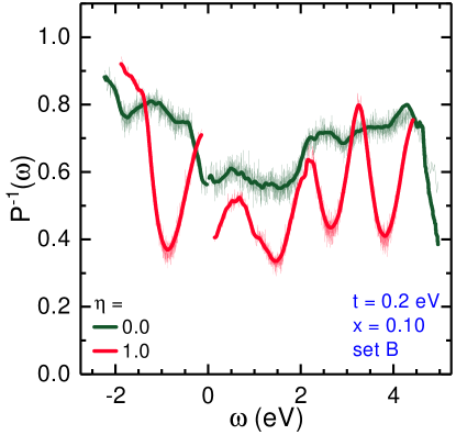
Figure 18: Spectral function of the inverse participation number $P^{-1}(\omega)$ (24) for parameter set $B$ of Table 1 and $t=0.2$ eV at $x=10$%. The thick red curve stands for the fully screened case $\eta=1$ and reveals the spatial extension jump at $\mu$, whereas, in the absence of $e$-$e$ interactions ($\eta=0$, thick green curve), the states directly below and above $\mu$ have the same spatial extension. Thin lines stand for the average $P_{n}^{-1}\left(\omega\right)$ vs $\omega=\langle\omega_{n}\rangle$.

Here, we are interested in the localization of the $n$-th HF eigenstate $\psi_{n,s}({\bf r})$ corresponding to the $n$-th HF eigenenergy $\omega_{n,s}$ both computed for the defect realization $s$. Therefore we shall explore the spectral function representing the statistically averaged IPN,

$$P^{-1}(\omega)=\frac{1}{M}\sum_{s=1}^{M}\left[\frac{1}{N_{s}(\omega)}\sum_{n}P_{n,s}^{-1}\delta(\omega-\omega_{n,s})\right],$$ (24)

where $P_{n,s}^{-1}$ is the IPN computed for $\psi_{n,s}({\bf r})$ and $N_{s}(\omega)$ is the DOS of the $s$ defect realization. It is worth noting that the division by $N_{s}(\omega)$ is problematic in regions with small DOS, which are of particular interest to us. Therefore, we analyze the essentially equivalent quantity,

$$P_{n}^{-1}\left(\omega=\langle\omega_{n}\rangle\right)=\frac{1}{M}\sum_{s=1}^{M}P_{n,s}^{-1},$$ (25)

where $\langle\omega_{n}\rangle=\frac{1}{M}\sum_{s=1}^{M}\omega_{n,s}$. This quantity has the great advantage to avoid the pathological division by the DOS $N_{s}(\omega)$ and displays in addition the fluctuations due to the many defect realizations in $\left\{P_{n,s}^{-1}\right\}$ and in $\left\{\omega_{n,s}\right\}$.

The fluctuations of the inverse participation number $P_{n}^{-1}$ for close-by energies $\langle\omega_{n,s}\rangle$ turn out surprisingly small as can be seen in Fig. 18 which displays two data sets, one without ($\eta=0$) and another with ($\eta=1$) $e$-$e$-interactions. At first glance, it is clear that both sets represent well localized wave functions over the whole spectrum. Note that a value $P^{-1}\approx 0.5$ corresponds to a wave function delocalized over two sites. It is important to note here that the localization is entirely due to the disorder, as a calculation without any defects yields $P^{-1}\approx 1/L^{2}$ (not shown), where $L$ is the linear dimension of our cluster. The $1/L^{2}$-dependence is consistent with the 2D nature of Bloch states of the $t_{2g}$ electrons in our system.

The striking difference of the two data sets in Fig. 18 reflects the absence or presence of the screening by $t_{2g}$ electrons. Without $e$-$e$-interactions, the monopolar defect potentials are not screened and hence the disorder effect is stronger; this is already manifest in the larger width of the LHB in the DOS. In the screened case instead, the Hubbard bands are much narrower both in the DOS, but also in the IPN distribution. The smaller values of IPN in the center of the Hubbard bands for $\eta=1$ indicate that these states are definitely more delocalized when the defect potentials are screened. In the $\eta=1$ case, it is worth noting that the defect states are much more localized, for instance in the energy region of the $c^{*}$ satellite, in comparison to the states in the center of the Hubbard bands, which are less affected by the random defect potentials and therefore show a smaller IPN.

The IPN of defect states inside the MH gap shows several interesting features. In the unscreened case $\eta=0$, the inverse participation number is approximately constant ($P^{-1}\approx 0.6$) for the states close to the chemical potential. This case corresponds to the DOS linear in $\omega$ in Fig. 15. For the screened case $\eta=1$, however, we observe a pronounced discontinuity in the degree of localization of defect states right below and above $\mu$, as seen in Fig. 18. The discontinuity in the degree of localization of the defect states at the chemical potential reflects the different nature of the electron removal and addition states in presence of $e$-$e$ interactions. It is evident from Fig. 18 that the removal states are more localized than the addition states.

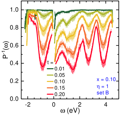
Figure 19: Spectral function of the inverse participation number $P^{-1}(\omega)$ (24) for parameter set $B$ of Table 1, $t=0.01$, 0.05, 0.10, 0.15, and 0.20 eV (green to red) and $\eta=1$ at $x=10$% (thick lines). Thin lines stand for the average $P_{n}^{-1}\left(\omega\right)$ vs $\omega=\langle\omega_{n}\rangle$.

In Fig. 19, we explore the $t$ dependence of the IPN for the case with $e$-$e$ interactions ($\eta=1$). We recognize that in the regime of small $t$ (close to the atomic limit) $P^{-1}\approx 1$. That is the electron states are perfectly localized at a single site, as one expects for the classical case $t=0$. The upper limit $P^{-1}=1$ shows that our definition of the IPN in the spin and orbital degenerate case is correct. The choice of a small finite hopping $t=0.01$ eV in Fig. 19 is dictated by the dependence on $t$ of the computation time: the smaller $t$ is the longer it takes to reach convergence. We see that the defect states close to $\mu$ and those at the bottom of the LHB are slightly more delocalized. For these defect states, IPN is in the range $P^{-1}\in(0.8,1.0)$. This weak delocalization at small $t$ is a consequence of the motion of the holes on the active bonds and increases with increasing $t$. We also see that the states in the center of the various Hubbard subbands delocalize faster with increasing $t$ than the defect states in between the Hubbard multiplets. Thus, we can conclude that all states remain well localized even at the moderate doping concentration of $x=10$% and for the typical value $t=0.2$ eV of the hopping integral in these materials.

VII Spin-orbital polarons and reduction of magnetic and orbital order

From the study of the IPN in the previous Section, it naturally follows that: (i) the defect states must be visualized as localized small polaron states that are tightly bound to defects and (ii) the symmetry of each polaron state relative to the closest defect must be strongly broken. It is important to contrast here two distinct physical sources of localization in condensed matter physics:

• Wave functions localize (i.e., their spatial extension undergoes an extreme reduction) due to the presence of defects or of any kind of disorder, as it happens, for instance, to the single particle states in the Anderson localization scenario Anderson (1958); Lee and Ramakrishnan (1985).

• On the other hand, electrons localize also due to strong (local) $e$-$e$ interactions as in the half-filled Hubbard model, that is in the absence of disorder Mott (1974).

In general, the Anderson and the Mott routes to localization, as listed above, are expected to combine in very non-trivial ways Braganca et al. (2015). In the regime of strong correlations, $t\ll U$, the ground state of the Hubbard model at half-filling is a Mott insulator with AF spin correlations. Added holes create spin defects while moving in the AF spin background, and form spin polarons Martinez and Horsch (1991); Wróbel et al. (2008). The motion of the hole inside the polaron cloud represents the main kinetic energy. Yet, as found for instance in the high-$T_{c}$ materials, the entire polaron may in addition perform a coherent motion on the magnetic energy scale $J\propto t^{2}/U$ Martinez and Horsch (1991).

In the case of orbital polarons in a state with AO order, the holes have an even stronger tendency towards localization, for instance in systems with $t_{2g}$ orbital degrees of freedom Daghofer et al. (2008); Wohlfeld et al. (2008); Wróbel and Oleś (2010). A similar analysis of individual hopping processes as for spin polarons Bała and Horsch (2005); Wróbel et al. (2008) is possible and provides a good insight both into the optical excitations Wróbel et al. (2012) and the spectral properties van den Brink et al. (2000); Daghofer et al. (2004); Brzezicki et al. (2014); Bieniasz et al. (2016) of orbital systems. More demanding is the theoretical description of a charge added to a system where both spin and orbital order alternates and excitations of both types of degrees of freedom may contribute to the polaron cloud Zaanen and Oleś (1993); Bieniasz et al. (2017). Results depend on the actual symmetry of the spin and orbital order realized in the ground state. Theoretical studies have shown that single SO polarons in systems where both spins and $t_{2g}$ orbitals alternate, as in the $(a,b)$ planes of the vanadium perovskites, tend to localize Wohlfeld et al. (2009); Berciu (2009).

Experimentally, such polarons were first identified in half-doped manganites for $e_{g}$ orbital degrees of freedom Kim et al. (2002); Yamauchi and Picozzi (2013), but exist also in doped cobaltates Daghofer et al. (2006) and in the cubic vanadates Reehuis et al. (2016). In the latter case, being of interest here, the doped holes move in the spin-orbital ordered $C$-AF/$G$-AO state and the emerging SO polarons perturb both spin and orbital order. These polarons are bound to the charged defects: this eliminates any coherent motion and the perturbation of the spin-orbital order in the system can be described by means of a detailed analysis of the nature and of the structure of the polaron cloud, see below. Thus, the polaron cloud provides a many-body measure of the reduction of the spin- and orbital- order parameter as function of doping. In this Section, our aim is to define the SO polaron wave function and to explore the spatial extension, or the IPN of the SO polaron.

In the spin- and orbital- ordered state, it is convenient to expand the polaron wave function $|\psi_{n}({i})\rangle$ in a string basis,

$$|\psi_{n}({i})\rangle=\sum_{{\mathbf{\delta}},\alpha}a_{n,\alpha}({\mathbf{\delta}})|{i+\delta};S_{\alpha}({\mathbf{\delta}})\rangle,$$ (26)

where the label $n$ distinguishes polaron states that may differ by their spatial symmetry and their spin. However, in the following, we shall consider only the polaron state with the minimal energy. The wave function of the polaron $|\psi_{n}({i})\rangle$ is centered or has its largest amplitude at the vanadium site $i$. Its kinetic energy involves the neighboring sites $\{i+\delta\}$, on varying ${\bf\delta}=\sum_{m=1}^{n(\alpha)}{\bf\delta}_{m}$, as the hole propagates along different paths, $S_{\alpha}({\delta})=\{{\mathbf{\delta}}_{1},{\mathbf{\delta}}_{2},\dots,{\mathbf{\delta}}_{n(\alpha)}\}$, where ${\bf\delta}_{m}=\pm e_{\nu}$ and $\nu=x,y,z$ are the unit vectors of the cubic lattice. A string state, $|{i+\delta};S_{\alpha}({\mathbf{\delta}})\rangle$ in Eq. (26), corresponds to the state of a hole after it has moved along a particular path $S_{\alpha}(\delta)$ from site $i$ to site $i+\delta$ and, therefore, it automatically contains information about the spin and orbital defects created along that particular path. Next, we proceed as in the case of the localization of single particle wave functions and define the IPN for the many-body wave functions of SO polarons as

$$P_{n}^{-1}=\sum_{{\bf\delta}}\left(\sum_{\alpha}|a_{n,\alpha}(\delta)|^{2}\right)^{2}.$$ (27)

As each path $S_{\alpha}({\bf\delta)}$ corresponds to a sequence of spin-flips and/or orbital changes relatively to the underlying spin-orbital ordered background, the energy of a string state increases with the length of the related path and only short paths and related string states contribute effectively as long as the system is not close to a phase transition.

In the dilute case (i.e., small density $x=n_{h}/N_{a}$ of doped holes), the overall reduction of the local magnetic order parameter $m^{s}$ can be calculated from the spin deviation $m^{sP}$, with respect to the underlying spin-orbital ordered background associated with a single polaron,

$$m^{s}\simeq m_{0}^{s}-xm^{sP},$$ (28)

where $m_{0}^{s}$ is the local magnetization in the undoped ground state, as we can imagine that the interactions between polarons are negligible. Then, $m^{sP}$ can be computed by means of the many-body wave function of the SO polaron,

$$m^{sP}=\langle\psi_{0}|\hat{m}^{s}({Q})|\psi_{0}\rangle-\langle\psi({i})|\hat{m}^{s}({Q})|\psi({i})\rangle.$$ (29)

Here, $|\psi_{0}\rangle$ is the $N$-particle ground state of the underlying spin-orbital ordered background and $|\psi(i)\rangle$ is a single-polaron wave function in the space of $(N-1)$ particles.

In this Section, we analyze the localization from the strong correlation perspective. It is evident from the uHF results for the IPN in Fig. 19 that all states of the system are perfectly localized in the limit $t\rightarrow 0$. With increasing $t$ the states become gradually more extended. Accordingly, an important probe for the delocalization is the decrease of spin and orbital order parameters $m^{s}$ and $m^{o}$, respectively. The staggered spin order of the $C$-AF structure, for example, is measured by

$$\hat{m}_{\nu}^{s}(Q)\equiv\sum_{j}\hat{m}_{j,\nu}^{z}e^{iQ\cdot j},$$ (30)

where $j$ and $\nu=a,b,c$ are site and orbital flavor indices, respectively. In the following, we use the convention $\hat{m}^{z}=2\hat{S}^{z}$, where $\hat{S}^{z}$ is the $z$-component of a spin-$1/2$ operator. The staggered orders of $C$ and $G$ states are measured by modulation vectors $Q_{C}=(\pi,\pi,0)$ and $Q_{G}=(\pi,\pi,\pi)$, respectively. Furthermore, within the uHF approach, it is straightforward to distinguish the contributions from $ab$- and $c$- electrons to the order parameters, respectively. Thus

$$m^{s}=m_{ab}^{s}+m_{c}^{s},$$ (31)

where $m_{\nu}^{s}=\langle\hat{m}_{\nu}^{s}({Q_{C}})\rangle$ for $C$-type spin order. Similar construction applies for the $G$-type orbital order parameter, $m_{\nu}^{o}=\langle\hat{m}_{\nu}^{o}({Q_{G}})\rangle$.

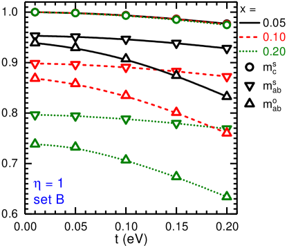
Figure 20: Self-consistent uHF results for the spin-order parameters $m_{c}^{s}$ and $m_{ab}^{s}$ and the orbital-order parameter $m_{ab}^{o}$ for the $C$-AF/$G$-AO ordered phase resulting from electrons in $a/b$ and $c$ orbitals, respectively, as functions of the hopping parameter $t$ and for different doping concentrations $x=0.05,0.10,0.20$.

In Fig. 20, the $t$ dependence of the spin-order parameters $m_{ab}^{s}$ and $m_{c}^{s}$ and of the orbital-order parameter $m_{ab}^{o}$ are shown. As we already explained above, hole doping concerns the $\{a,b\}$ orbital doublet and the magnetic moment component $m_{ab}^{s}$ is thus reduced by $x$ at $t=0$, whereas $m_{c}^{s}=1$ remains unchanged as there is no doping into $c$ orbitals. On increasing $t$, holes move and the spin and orbital order are further reduced. This effect is particularly small for $c$ orbitals, as their motion involves only doubly occupied $c^{2}$ configurations and, therefore, costs the intraorbital Hubbard repulsion $U$. The contribution of such processes is small in comparison to that of the virtual processes involving $a$ and $b$ electrons. In Fig. 20, one recognizes a strong reduction of the orbital order $m_{ab}^{o}$, both as a function of $x$ and $t$. In fact, the kinetic processes have a stronger effect on the $G$-type orbital order parameter $m_{ab}^{o}$ than on the $C$-type spin order $m_{ab}^{s}$. This may be seen as a precursor of the trend observed in the experiments performed on La_1-xSr_xVO₃ Miyasaka et al. (2000) where the $G$-AO order melts at a lower doping than the $C$-AF spin order.

Next, we shall use the order parameter expressions, derived in Appendix B by assuming non-interacting small SO polarons, for the interpretation of the uHF results. The central assumption is the linearity in $x$ of the order parameter corrections, which is confirmed by the present uHF results in a wide doping range, see Appendix B. It is important to recognize that in the insulating regime that we are considering, each small polaron is bound to and strongly deformed by the central charged defect. Thus, the number of relevant paths for the doped holes are significatively reduced in comparison to those available for a polaron not attached to a defect. Furthermore, the polaron state is strongly influenced by the random fields resulting from the other more-distant defects.

The expressions for the spin and orbital deviations associated with a single polaron are derived by considering the polaron cloud of a hole located on an active bond close to a defect. It is the FM correlations along the $c$-direction in $C$-AF structure in combination with the defect potential, which defines the direction of the active bond, that yields the dominant gain of kinetic energy for the hole. The virtual motion of holes in $a$ or $b$ direction is instead quenched by AF correlations. Thus, the polaron wave function is characterized by two physical parameters, namely: (i) the polarity parameter of the active bond $\delta_{c}$, where $\delta_{c}=0$ describes a hole localized on a single site, as for $t=0$, and $\delta_{c}=1/2$ an equal partition between the two sites of the active bond, as in the case of large $t$ and screened far-defect potentials ($\eta=1$); (ii) the activation energy $e_{0}$ of the virtual string excitations. We focus here on the spin- and orbital- order parameter due to $a/b$ orbitals that show the strongest dependence on doping:

$$m_{ab}^{s} \cong 1-x\left[1+\frac{2\left(t/e_{0}\right)^{2}}{1+\left(t/e_{0}\right)^{2}}\right],$$

$$m_{ab}^{o} \cong 1-x\left[1+2\delta_{c}+\frac{2\left(t/e_{0}\right)^{2}}{1+\left(t/e_{0}\right)^{2}}\right].$$ (32)

For an isolated single defect, the activation energy $e_{0}$ is given by Hund’s coupling $J_{H}$, whereas $\delta_{c}$ is controlled primarily by $t$ and the Jahn-Teller coupling. In the presence of disorder, the potentials due to the random far defects affect quite strongly both the activation energy $e_{0}$ and the polarity parameter $\delta_{c}$. Accordingly, these parameters are taken here as natural variational parameters. When we apply these relations to the uHF results, obtained as a statistical average over many defect realizations, we obtain for $\delta_{c}$ and $e_{0}$ the values of a typical bound small polaron.

Figure 21 shows the typical polaron parameters obtained by fitting the uHF results shown in Fig. 20 for the spin and orbital order parameters, $m_{ab}^{s}$ and $m_{ab}^{o}$, see Eqs. 32 (see also Appendix B). We find a significant increase of the activation energy $e_{0}$ from $0.33$ eV at $x=5$% to $0.82$ eV at $x=25$%. This increase can be attributed to the increase of the overall random potential strength on the single defect cube when the concentration of defects becomes larger and larger. We note that Hund’s exchange, which is the energy scale $e_{0}$ for an isolated defect as already mentioned above, is $J_{H}=0.6$ eV for parameter set B of Table 1.

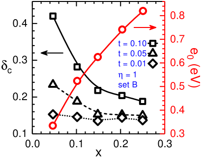
Figure 21: Doping dependence of the polaron superexchange energy scale $e_{0}$ and of the polarity parameter $\delta_{c}$ of a typical active bond for different values of $t$ (in eV) and parameter set B of Table 1. The lines are simply guides to the eye.

The interpretation of the data for the polarity parameter $\delta_{c}$ is more subtle. Here we determine $\delta_{c}$ directly from the data in Fig. 20 via the difference of $m_{ab}^{o}$ and $m_{ab}^{s}$ using Eqs. (32). The parameter $\delta_{c}$ naturally depends on $x$ and on $t$; large $t$ favors an equal distribution on the active bond, that is $\delta_{c}=0.5$. At small doping, this is almost realized for $t=0.1$ in Fig. 21 since the random polarization fields (i.e., the far-defect potentials) are quite small in this case. It is worth noting that, in the low doping regime, the small Jahn-Teller potentials, which naturally lead to an imbalance, become also relevant.

By means of the same small-polaron wave function for a hole on an active bond, we obtain for the IPN, with the help of the definition in Eq. (27),

$$P_{a}^{-1}\cong\left(1-2\delta_{c}+2\delta_{c}^{2}\right)\left[1-\frac{2\left(t/e_{0}\right)^{2}}{1+\left(t/e_{0}\right)^{2}}\right].$$ (33)

The finite polarity parameter $\delta_{c}$ explains the deviation of the IPN from $1$ in the small $t$ case for the states in the soft gap close to the chemical potential (see Fig. 19). The overall $t$-dependence of the IPN close to $\mu$ is determined both by the $t$-dependence of the polarity parameter $\delta_{c}(x,t)$ and by the virtual-string contributions in the polaron wave function. Interestingly, the nonlinear corrections driven by the random polarization fields via the $x$-dependence of $e_{0}$ and $\delta_{c}$ are particularly pronounced at small $x$ values (see also Appendix B).

In this Section, we have focused on the microscopic character of the defect states that are responsible for the formation of the soft gap and the reduction of spin and orbital order. We have shown that the SO polaron states inside the MH gap have a reduced spatial symmetry and are more strongly localized than the states in the center of the Hubbard bands. The polaron states in the soft gap are controlled by the randomness of the defect locations and by the interplay of kinetic energy and $e$-$e$ interactions.

VIII Relation to the PES of La_1-xCa_xVO₃

Now, we turn to the questions how the structure of the DS gap is affected by strength of the defect potential $V_{D}$ and whether we can identify characteristic defect-related features in the doping dependence of existing PES data. We shall explore here the PES spectra of La_1-xCa_xVO₃ since for this system Maiti and Sarma Maiti et al. (1998) have measured the doping dependence up to $x=0.5$, and moreover both PES and IPES spectra exist for the parent compound LaVO₃ Maiti and Sarma (2000). The latter yields clear evidence of the multiplet structure and provides an estimate for Hund’s exchange $J_{H}$ (see Fig. 2). Moreover, these spectra give us a measure for the principal parameter for the Mott gap $U-3J_{H}\approx 2.7-3.0$ eV between the centers of the LHB and the HS multiplet of the UHB. In the following study, we shall use $U-3J_{H}=3.0$ eV as determined after Maiti et al. Maiti and Sarma (2000) (set $C$ of Table 1). Another important energy scale that follows from PES experiments is the distance of the chemical potential from the center of the LHB, $\mu-E_{\rm LHB}$. Surprisingly, over the whole doping range in La_1-xCa_xVO₃, up to $x=0.5$, this scale is approximately constant, $\mu-E_{\rm LHB}\approx 1.5$ eV. Since it is the repulsive defect potential that pulls the $d^{2}$ defect states upward out of the LHB, we expect also an upward shift of the chemical potential. Therefore the distance of the chemical potential from the LHB center is expected to scale with the parameter $V_{D}$ in the Hamiltonian Eq. (1).

At this point, it is interesting to note that the pioneering work of Mott Mott (1974) in the 1970s on the metallic and nonmetallic states of strongly correlated matter was to some extent stimulated by the experiments of Dougier and Hagenmuller Dougier and Hagenmuller (1975), who explored the electrical conductivity of LaVO₃ doped with strontium. The metal-insulator transition in this compound at $x_{c}\approx 0.23$ was attributed to an Anderson type transition between localized and delocalized states in an impurity band. The option of a Mott gap in the defect band was ruled out Mott (1989). The presence of a soft gap with $N(\mu)=0$ in the insulating regime has not been considered.

So far, we have analyzed spectral functions in Secs. IV.1-VI using parameter set $B$ of Table 1. They have the advantage that satellite structures are well resolved, representing the atomic multiplet excitations. Interestingly, we see from spectra in Fig. 6, calculated with inclusion of $e$-$e$ interactions, that the LHB center remains at a fixed distance relative to the chemical potential for all doping concentrations, as required by the above experiments. However, parameter set $B$ implies $U-3J_{H}=2.2$ eV and $\mu-E_{{\rm LHB}}\simeq 0.8$ eV being both too small and thus not appropriate for the La_1-xCa_xVO₃ compounds.

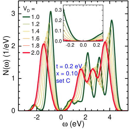
Figure 22: Density of states for $x=10$% and six different defect potentials $V_{{\rm D}}\in[1.0,2.0]$ eV. The data shows that the distance between the LHB and the chemical potential (at $\omega=0$) is increasing with $V_{{\rm D}}$ while the distance between the LHB and the HS state of the UHB stays constant. Parameters are $t=0.2$ eV and set $C$ of Table 1. The defect potential is of Coulomb type and $e$-$e$ interactions are included ($\eta=1$).

In Fig. 22, we display the $V_{D}$ dependence of the DOS for $U-3J_{H}=3.0$ eV appropriate for La_1-xCa_xVO₃ (set $C$ of Table 1) at $x=10$% doping. The resulting $N(\omega)$ spectra depend strongly on the $V_{D}$ parameter, Eq. (3), which determines both the strength of the Coulomb like defect potentials and the strength of $e$-$e$ interactions, Eq. (4), guaranteeing charge neutrality. On increasing $V_{D}$ from 1.0 to 2.0 eV, we recognize: (i) the DS gap becomes wider and softer; (ii) the characteristic energy scale $\mu-E_{\rm LHB}$ increases; (iii) the $d^{1}\rightarrow d^{0}$ satellite moves closer to the LHB and gets gradually absorbed. Moreover, (iv) the defect states right above the chemical potential ($\mu=0$), which are well separated from the HS UHB at $V_{D}=1$ eV, merge with this latter for $V_{D}=2$ eV; and (v) the gaps between the multiplets of the UHB get gradually filled with defect states as $V_{D}$ increases. Finally, we see that it requires a value $V_{D}\approx 2$ eV until one reaches the experimental value $\mu-E_{\rm LHB}\approx 1.5$ eV. One also notices in Fig. 22 that the energy between the center of LHB and the HS state of the UHB remains unchanged $U-3J_{H}=3.0$ eV for the different values of $V_{D}$, as expected from Table 2. That is, the intra-atomic excitations and multiplet splittings are not affected by the disorder.

The $V_{D}$ dependence of several characteristic single particle excitations $\omega_{m}$ relative to the chemical potential ($\mu=0$) are plotted in Fig. 23. The characteristic energies $\omega_{{\rm LHB}}=E_{\rm LHB}-\mu$ as well as the satellite energies, $\omega_{c^{*}}$ and $\omega_{S}$ have been determined by a fit with three Gaussians to the spectra in Fig. 22 at negative energy. The linewidths are indicated by shading. In order to understand the variation of $\omega_{{\rm LHB}}=E_{{\rm LHB}}-\mu$ we need an estimate for the dependence of $E_{{\rm LHB}}$ and $\mu$ on the defect potential $V_{D}$. The center of the LHB corresponds to a $d^{2}\rightarrow d^{1}$ transition. In uHF, this energy is connected with the removal of the topmost occupied $a$ (or $b$) electron of a $d^{2}$ configuration far away from a defect,

$$E_{{\rm LHB}}\simeq\epsilon_{a}+U-3J_{H}.$$ (34)

The chemical potential can be approximated by a similar excitation in the direct neighborhood of a defect, that is at a spectator site. Hence

$$\mu\approx\epsilon_{a}+U-3J_{H}+V_{D},$$ (35)

and therefore

$$\omega_{{\rm LHB}}=E_{{\rm LHB}}-\mu\approx-V_{D}.$$ (36)

This simple estimate reproduces qualitatively the trend of the full self-consistent uHF result in Fig. 23 that is $\omega_{{\rm LHB}}\approx-0.8V_{D}$. The small deviation is not unexpected since both $E_{{\rm LHB}}$ and $\mu$ will acquire upward shifts from the long-range tails of the defect potentials leading to a small positive correction proportional to $V_{D}$ in $E_{{\rm LHB}}-\mu$.

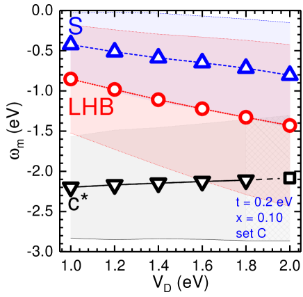
Figure 23: Characteristic energies $\omega_{m}$ of the spectral features resolved below the chemical potential $\mu$ ($\omega=0$) as functions of the defect potential $V_{{\rm D}}\in[1.0,2.0]$ eV: the center of gravity of the LHB (LHB, red circles), the filled defect states (S, blue up-triangles), and the satellite due to hole states ($c^{*}$, black down-triangles and square). The energies and the linewidths (indicated by the shaded areas colored according to the symbol colors) were determined by fitting the data in Fig. 22 with three Gaussians, respectively. The $c*$ data for $V_{D}=2.0$ eV (black square) has been obtained by linear fitting the data for $V_{D}<2.0$ eV as there was no possibility to resolve such peak within the overall LHB peak.

The satellite $c^{*}$ corresponds to a $d^{1}\rightarrow d^{0}$ transition and is a fingerprint of the spin-orbital polaron state. As we discussed before the doped hole selects an active FM bond $\langle i,j\rangle$ parallel to $c$ next to a defect. The random defect fields tend to localize the hole on a single site $i$ leading to a configuration $|c_{i},(c_{j}a_{j})\rangle$ where the single $a$ electron is on site $j$ of the active bond. This is described by the polarization parameter $\delta_{c}=0$. If the kinetic energy (i.e., $t$) is strong enough, the $a$ electron delocalizes on the active bond leading to $\delta_{c}=0.5$. The annihilation energies of $c$-electrons in the two configurations relative to the chemical potential $\mu$ are

$$\omega_{c^{*}} \simeq \epsilon_{c}-\epsilon_{a}-(U-3J_{H})(1-\delta_{c}),$$ (37)

$$\omega_{S} \simeq \epsilon_{c}-\epsilon_{a}-(U-3J_{H})\delta_{c}.$$ (38)

Most importantly, in the expression of $\omega_{c^{*}}$, the dependence on the polarization parameter $\delta_{c}$ contributes with a large prefactor $U-3J_{H}$. Therefore, the delocalization of the remaining $a$-electron in the small polaron is reflected in a large energy shift of the $c^{*}$ satellite. That is, the state of the $a$ electron can be probed by annihilation of $c$-electrons. Comparing the expression $\omega_{c^{*}}$ with the data in Fig. 22 yields $\delta_{c}\simeq 0.3(0.33)$ at $V_{D}=1(2)$ eV, respectively. There is no direct $V_{D}$ dependence in these expressions. The origin of the small change of $\delta_{c}$ observed above is unclear.

As one can see in Figs. 22 and 23, the widths of both the LHB and the UHB increase with increasing defect potential $V_{{\rm D}}$. Since the corresponding spectra are calculated for fixed doping $x=0.1$ and constant kinetic energy parameter $t$, the broadening can be directly attributed to the increasing randomness resulting from the stronger long-range disorder potentials. Moreover, we see that, at small $V_{{\rm D}}\simeq 1.0$ eV, the $d^{1}\rightarrow d^{0}$ satellite excitations $\omega_{c^{*}}$ are well separated from the $d^{2}\rightarrow d^{1}$ excitations at $\omega_{{\rm LHB}}$ that define the LHB. Due to the $V_{D}$ dependence of the LHB, see Eq. (36), the $c^{*}$ satellite penetrates the LHB at $V_{D}\approx 1.6$ eV. In other words, the $d^{0}$ final state on the active bond becomes unstable and changes into a $d^{1}$ state by a simultaneous $d^{2}\rightarrow d^{1}$ transition at a vanadium host site not belonging to the defect cube. With the onset of the delocalization of holes, we come to the borderline of the regime of well localized spin-orbital polarons. The delocalization of holes has severe consequences for the uHF algorithm and leads to a slowing-down of convergence of the algorithm, that is, for large $V_{D}$ when the $c^{*}$ satellite disappears in the LHB.

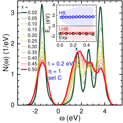
Figure 24: Density of states $N(\omega)$ as a function of increasing doping concentration $x\in[0.02,0.50]$ for set $C$ of Table 1 including $e$-$e$ interactions ($\eta=1$) and for $t=0.2$ eV. Inset displays the small variation with $x$ of the distance of the peak of LHB from chemical potential $\mu$ ($\omega=0$): experimental results of Maiti and Sarma for La_1-xCa_xVO₃ Maiti et al. (1998) (black squares); theoretical data for the LHB (red circles) and the HS state of the UHB (blue pentagons). The shaded areas colored according to the symbol colors give a measure of the linewidths of the related multiplet structures.

The doping dependence of the uHF DOS for La_1-xCa_xVO₃ is displayed in Fig. 24. These calculations were performed using long-range $e$-$e$ interactions ($\eta=1$) and interaction parameters, $U-3J_{H}=3.0$ eV and $V_{D}=2.0$ eV (see parameter set $C$ in Table I). As most important features on the PES side of the spectra we note: (i) the persistence of a soft DS gap up to large doping, and (ii) the essentially doping independent distance of the chemical potential from the center of the LHB, as found in the experimental data of Maiti and Sarma Maiti et al. (1998). Unfortunately, the existing experimental data do not allow to draw a conclusion with any certainty concerning the existence of a $c^{*}$ satellite. Thus, it remains as a challenge for future higher resolution experiments to see whether this feature can be resolved. The inset highlights the independence on doping of $\mu-E_{\rm LHB}\approx 1.4$ eV and of the fundamental Hubbard gap $(U-3J_{H})$. The decrease of the spectral weights with doping is consistent with the sum rules discussed in Sec. IV.

We observe a pronounced shift of spectral weight in the UHB towards lower energies as a function of doping, i.e., resulting in an increase of the spectral weight in the regime of HS excited states. At large doping, the multiplet structures of the UHB begin to merge and, as a consequence, the UHB becomes almost featureless. The multiplet excitations lose their distinct character as (for these parameters) these excitation processes are degenerate with $d^{1}\rightarrow d^{2}$ excitations at hole sites. Moreover, we note that the $d^{1}\rightarrow d^{2}$ transitions have a narrower width of their multiplet structure compared to that for the $d^{2}\rightarrow d^{3}$ transitions of the host.

In Fig. 24, we recognize a moderate increase of the width of the LHB with increasing defect and doping concentration. This one may have expected since there are two prevailing mechanism that contribute to an additional broadening of the LHB when the doping concentration is increased. Namely, (i) there are the growing satellites $c^{*}$ and $S$ that contribute to the increase overall width of the LHB, and (ii) due to the increasing doping concentration, the defects get closer and thereby the disorder fluctuations are expected to increase. There is, however, also a counteracting effect due to an increased screening resulting from the defect states and the narrowing of the soft gap. We note that this screening, which is still non-metallic, is fully included in our calculation, due to the finite field method we are using. We also remark that, in terms of an alternative random phase many-body theory, our treatment of $e$-$e$ interactions for the $t_{2g}$ subsystem would correspond to the calculation of the full dielectric matrix Horsch and von der Linden (1988) for an inhomogeneous and random system. The complex dielectric matrix would then yield a quite similar or even the same polarization charge density induced by the defect potentials as in our uHF calculations. This perspective highlights that the dielectric screening in systems with defect states and soft gaps is rather involved and, to the best of our knowledge, it has not been addressed yet by any many-body theoretical approach.

IX Discussion and summary

This work elucidates the inherent complexity of charged defect states in orbitally-degenerate Mott insulators. We have studied a generic three-band model representing the $t_{2g}$ electrons of the vanadium ions that guarantees a faithful description of the magnetic and orbital ordered phases of the vanadium perovskites such as LaVO₃ or YVO₃. The model developed here includes the local Hubbard-Hund interactions and the long-range $e$-$e$ interactions. Therefore, it describes the dielectric screening of the Coulomb potentials of the random charged defects due to the $t_{2g}$ electrons explicitly in the regime of strong electron correlations. Nevertheless, there are relevant interactions that we have omitted, such as spin-orbit and orbital polarization interactions, as discussed in Sec. II. We have neglected such terms to achieve a closer correspondence to the generic models used in studies of disorder such as the quantum Coulomb glass or the Anderson-Hubbard model. Our model may be thus seen as multiflavor generalization of these models.

The calculation of the one-particle excitation spectra of a Mott insulator with orbital degeneracy and random defects is a complex task that was only possible to undertake within the unrestricted Hartree-Fock approximation. We stress that this is the only scheme able to: (i) control simultaneously the strong correlations, the Coulomb interactions and the randomness of defects even at high doping and (ii) reproduce the essence of Mott physics, i.e., the atomic multiplet structure and the variation of the spectral weights in the Hubbard bands. A more detailed description of the algorithm used for the treatment of disorder is given in Appendix A. There, we also display a subtle convergency test for our algorithm and show that the gradual switching on and off of $e$-$e$ interactions leads basically to the same statistical average for the density of states $N(\omega)$ as for the initial state.

An important feature of the vanadium perovskites is the robustness of the Mott-Hubbard gap and of the spin and orbital order up to high doping concentrations. Our unrestricted Hartree-Fock results for the single particle density of states $N(\omega)$ reveal the persistence of the atomic multiplet structure of V-ions up to doping concentrations as large as 50% in photoemission and inverse photoemission spectra. At the same time, there is a strong spectral weight transfer from the Hubbard bands into the Mott-Hubbard gap and into satellite structures of the lower Hubbard band and the multiplets of the upper Hubbard band. We have analyzed the energetics and the doping dependence of spectral weights of the different excitations in the atomic limit that provides valuable information for the insightful interpretation of photoemission spectra.

The opening of a gap in the defect states at the chemical potential $\mu$ inside the Mott gap is a subtle feature in doped Mott insulators. We have presented a very detailed analysis how $e$-$e$ interactions and the kinetic gap mechanism jointly contribute to the formation of the gap in defect states. As we have shown, the states in the defect states gap can be understood as small spin-orbital polaron states bound to defects. Note that, in the presence of $e$-$e$ interactions, these objects are electric dipoles that interact effectively via dipole-dipole interactions. The kinetic energy gain of the doped hole moving within the spin-orbital polaron on a ferromagnetic active bond is the origin of a level splitting at $\mu$ and thereby of the kinetic mechanism for the defect states gap formation. We have demonstrated that the defect states gap survives the disorder average and typically yields a soft gap.

Central role for the quantitative description of the insulating state is played here by a statistical analysis of the gap using a Weibull distribution as introduced in Ref. Avella et al. (2015). Using this tool we have shown that the exponent $\nu$ of the soft gap in $N(\omega)\propto|\omega|^{\nu}$ at the chemical potential is nonuniversal, that is, it depends sensitively on: (i) the strength of $e$-$e$ interactions and (ii) on the hopping parameter $t$ which controls the kinetic energy. In particular, we note here that in the atomic limit ($t=0$), $e$-$e$ interactions are not strong enough to produce a Coulomb gap in the vanadium perovskites, as one might expect on the basis of Efros-Shlovskii theory. Instead, we find in this regime exponents that rather correspond to a Coulomb or zero-bias anomaly $0<\nu<1$.

We have investigated the degree of localization of the unrestricted Hartree-Fock wave functions quantitatively. We used here as a measure the inverse participation number, which we have generalized for systems with spin and orbital flavors. In particular, we have found that the defect states in the soft gap are typically localized on one up to two sites, and they are more strongly localized than the states inside the Hubbard bands. This feature is surprising and the inverse participation number provides an independent proof for small spin-orbital polarons bound to defects. Interestingly, we observed a strong discontinuity in the localization of states right below and above $\mu$ in the presence of $e$-$e$ interactions, whereas in their absence no discontinuity could be found.

Using the unrestricted Hartree-Fock, we have calculated the doping dependence of spin- and orbital- order parameters in the $C$-AF/$G$-AO phase. Our results reveal a faster decrease of the orbital order as compared to the spin order. The ordered state persists beyond $x=0.5$ in our calculations. This robustness is an independent sign that doped holes form small polarons. Starting from the atomic limit, we have constructed the many-body wave function of a spin-orbital polaron bound to a defect. We have then established that the reduction of spin and orbital order obtained by unrestricted Hartree-Fock is consistent with that calculated with help of the many-body spin-orbital polaron state. We note that, for a quantitative comparison with existing experimental data for the reduction of spin and orbital order and the insulator to metal transition Fujioka et al. (2005); Reehuis et al. (2016), the inclusion of spin-orbit interaction and orbital polarization terms Avella et al. (2013) is required.

In photoemission experiments of gapped systems, the position of the chemical potential $\mu$ is determined by defects. For the doped cubic vanadates we find that $\mu$ lies in the center of the defect states gap that forms inside the Mott-Hubbard gap. The defect potential $V_{{\rm D}}$, which basically confines doped holes to a cube formed by the V ions being the nearest neighbors of a charged defect, provides a measure of the upward shift of the in-gap defect states relative to the lower Hubbard band Horsch and Oleś (2011). We found here that the distance of $\mu$ from the center of the lower Hubbard band scales linearly with $V_{D}$. Moreover, we found that this distance is basically unchanged by doping up to 50%, i.e., consistent with the photoemission study by Maiti and Sarma Maiti et al. (1998); Maiti and Sarma (2000) for La_1-xCa_xVO₃. We interpret this as a manifestation of small spin-orbital polaron physics. Furthermore, we have shown that the intensity of the $d^{1}\rightarrow d^{0}$ satellite of the lower Hubbard band, that grows proportional to the doping concentration $x$, provides a direct fingerprint of the trapped spin-orbital polarons. The position in energy of this satellite relative to the lower Hubbard band and its width yields detailed information about the polarization of the SO polaron and the strength of random defect fields. For the La_1-xCa_xVO₃ system, we found that the satellite is not well separated from the lower Hubbard band and thus has not been resolved in the existing PES experiments so far. Certainly, it would be very interesting to have high resolution photoemission or tunneling experiments carried out on this compound.

It is important to stress that our model, which includes simultaneously the defect Coulomb potential and the $e$-$e$ interactions, is qualitatively different from the Coulomb glass type of models not just because it contains orbital and spin degrees of freedom. The Coulomb glass model contains only a random distribution of defect state energies, thus the dipole (negative defect charge and positive bound hole) formation cannot take place. It is just this latter feature that makes an important difference between the results obtained by these two types of defect modelization (ours being definitely more realistic) and that leads to a weakening of the disorder with increasing $e$-$e$ interactions. Instead, for Coulomb glass type of models, $e$-$e$ interactions enhance localization Pollak (2012).

Summarizing, we have demonstrated a systematic redistribution of the spectral weights with increasing doping by charged defects in Mott insulators using the example of $R_{1-x}$Ca_xVO₃. Even when doping is rather high, these systems remain insulating and the large Mott-Hubbard gap accommodate the spectral weight due to defect states, with the filled and unfilled defect states separated by a kinetic gap. We have also shown that the treatment of defects in strongly correlated materials with orbital degrees of freedom requires important extensions of the Hubbard-Anderson model. We designed a well motivated model for systems with orbital degrees of freedom to uncover the origin of the satellite structures that appear in doped systems and to explain the corresponding sum rules. In this way, the interpretation of photoemission and inverse photoemission experiments on Mott insulators doped with charged defects becomes possible. We have also explained why the spectral features, which arise from different excitation processes, can be energetically very close or overlap with one another, making them unresolvable in the experimental spectra.

Finally, one may ask whether there is any fundamental difference between doping into the vanadadium perovskites and the cuprate high-$T_{c}$ transition metal oxides. In both cases the formal charge of the defects and the distance to the relevant electrons to the Cu or V ions, respectively, are similar. Nevertheless, in the cuprates, defects form shallow impurity states, whereas in the vanadates they are deep inside the gap. Our analysis shows that the additional orbital degree of freedom makes an important difference. The confinement of spin-orbital polarons in vanadates is typically on a single active bond, and thus is much stronger than the localization of spin polarons in cuprates. This also implies that the screening of defect potentials at low energy due to the defect states is weaker in vanadates, effectively leading to stronger binding of carriers and to a shift of the insulator-to-metal transition to much higher doping concentrations than in high-$T_{c}$ materials.

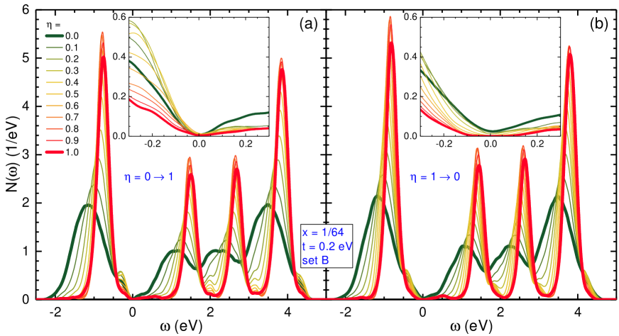
Figure 25: $t_{2g}$ DOS $N(\omega)$ as obtained for $t_{2g}$ states from $M=100$ random defect realizations for $t=0.2$ eV at doping $x=1/64$, and for: (a) increasing value of $e$-$e$ interaction (4) in steps of $0.1$ from $\eta=0$ (thick green line) to $\eta=1.0$ (thick red line), and (b) decreasing value of $e$-$e$ interaction (4) from $\eta=1.0$ (thick red line) to $\eta=0$ (thick green line). Insets show zooms of $N(\omega)$ near the Fermi energy at $\omega=0$. Other parameters as in set $B$ of Table 1.

Appendix A The algorithm to determine stable configurations with random defects

As we described in Sec. IV.1, we present results obtained by averaging over $100$ randomly chosen defect realizations. Any random defect realization is a configuration of defects defined by a set of randomly-chosen positions within the $R$ lattice of doped $R_{1-x}$Ca_xVO₃ that host the Ca defects. Such positions, in terms of Cartesian coordinates, are obtained by subsequent calls to a pseudo-random number generator. No constraint is imposed (e.g., no minimal distance between the defects is required) except for the obvious hard-core constraint that any site is singly occupied, either by an $R$ ion or by a Ca defect ion. The number of positions/defects in the set defines the degree of doping of the system $x$.

The employed Hartree-Fock self-consistency procedure is based on recursion: the values of all single-particle correlation functions appearing in the Hamiltonian are computed at each iteration after diagonalizing the Hamiltonian where the values computed at the previous iteration have been plugged in. The first iteration obviously requires externally-provided starting values (initialization), which are supplied on the basis of an educated guess. The recursion stops after a finite number of steps when all values in two subsequent iterations differ (actually the relative difference is used: $|x_{n-1}-x_{n}|/|x_{n-1}|$) at most by a chosen amount (i.e., $10^{-3}$). In order to speed up the convergence and to avoid long cycles involving states with almost identical energies and slightly different values of the single-particle correlation functions characterizing them, the actual new values at each iteration are built as a linear combination of the old ones and the ones effectively obtained by diagonalizing the Hamiltonian. The proportion among the two components starts quite low in favor of the old values (0.1) and increases steadily with the iterations up to exclude the old values from the combination within 200 steps.

The size of the system ($N_{a}=8\times 8\times 8$), the number of orbital and spin degrees of freedom per site ($6=3\times 2$), and the number of random defect realizations to statistically average upon (100) make the numerical calculations very demanding and unavoidable to parallelize the code in order to keep the convergence for a set of Hamiltonian parameters within one day. In the finite system of $N_{a}$ sites (atoms) considered here, we can change the defect concentration in steps of 1/512. For instance, the low doping of $x=1/64$ used in Fig. 25 corresponds to 8 random defects. Each of these defects defines a cube of V ions around it and, at the very beginning, one hole is doped to each cube. A priori, we have no information about the ultimate doped holes’ configuration for a given distribution of random defects, but the lowest energy configuration is self-consistently chosen to minimize the random fields acting on each hole.

The procedure developed to find this configuration is the following one: (i) we start from a neutral configuration (homogeneous doping of 1/8) at each corner of any cube surrounding a defect at $\eta=0$; (ii) increasing $e$-$e$ interactions we reach $\eta=1.0$ with full convergence at each value of $\eta$ along the path in the parameter space for each starting configuration of random defects; (iii) starting from the final point of (ii) [and, therefore, exactly for all the same random defect configurations] we reach $\eta=0$ with again full convergence at each value of $\eta$ along this path. But, in (ii) and/or in (iii), if the convergence was lost along the way [for a value of $\eta\in(0.0\to 1.0\to 0.0)$], a new random configuration was used. Accordingly, if one looks carefully and, in particular, in the zoomed inset, one will see that also $\eta=1.0$ is slightly different between the two panels (i.e., the two pathways) because of the last requirement.

The rebooting procedure is necessary to stabilize the final results: When a set of values for a given Hamiltonian parameter is explored, if the convergence is not reached from the initial value of the set to the final value of it, we generated another random defect realization and reboot the search in order to get a smooth progression per each random defect realization. This rebooting procedure allows one to avoid taking into account random defect realizations with extremely weird relative positions of the defects that would hinder the convergence and that would be anyway discarded by nature.

The algorithm described above is unbiased, but rather involved. Therefore, we present here a test of convergence carried out by performing the calculations at low doping, $x=1/64$ , and $t=0.2$ eV in two ways: (i) starting with the case of absent $e$-$e$ interactions ($\eta=0$) and gradual switching on the screening interactions up to $\eta=1.0$, and (ii) starting from the screened $e$-$e$ interactions at $\eta=1.0$ and reducing the screening down to $\eta=0$. It is worth noting that the calculation performed starting from monopole interactions ($\eta=0$) and reaching the state with screened $e$-$e$ interactions ($\eta=1.0$) leads to a physically very different state controlled effectively by dipolar interactions between defect centers, see Fig. 25(a). It is remarkable that the subsequent switching off of $e$-$e$ interactions leads back to essentially the same initial state, see Fig. 25(b). For such a complex landscape we are dealing with here, this is indeed a great result.

In fact, one finds very similar results independently of whether the $e$-$e$ interactions are increased or reduced, see Figs. 25(a) and 25(b). In both cases, the system is an insulator, with distinct structures representing the LHB and UHB. If $e$-$e$ interactions are absent ($\eta=0$), the maxima corresponding to the LHB and the HS/LS excitations in the UHB are wide and the states that correspond to the excitations at sites occupied by holes cannot be resolved from these peaks. When the $e$-$e$ interactions increase towards fully screened ones ($\eta=1.0$), the defect states appear instead at the lower edges of both the LHB and the HS subband in the UHB. Both figures are remarkably similar even for the zoomed DOS near the Fermi energy, where a broader gap is visible at $\eta=1.0$. This test confirms that the entire procedure, which includes the averaging over $M=100$ random defect realizations, is reliable and gives well converged and reproducible results.

Appendix B Bound spin-orbital polarons

In this Appendix, we shall analyze the reduction of the spin and orbital order parameters as functions of the doping $x$ and of the kinetic energy parameter $t$ in the frame of the spin-polaron theory. This strong coupling approach rests on the idea that, in the dilute limit, polaron-polaron interactions should be negligible due to the local nature of the polarons. This implies that the overall reduction of the order parameters can be determined in terms of the reduction induced by the polaron cloud of a single polaron, whose size scales with the kinetic energy parameter $t$. Accordingly, the overall reduction of the orders scales linearly with $x$, as in Eq. (28). Here, we shall first test up to which concentration $x$ and to which kinetic energy parameter $t$, the independent polaron picture holds by inspecting the uHF results for the respective order parameters. Next, we shall derive the wave function for a spin polaron bound to a defect using the string basis introduced in Sec. VII. Finally, we shall compare the $t$-dependence of the spin-polaron cloud with the order parameters calculated by the uHF method including the disorder. This will provide the basis for a qualitative and quantitative interpretation of the uHF results in the frame of the spin-orbital polaron theory emerging from the strong correlation picture.

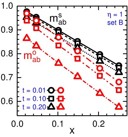
Figure 26: Contributions from electrons in $a/b$ orbitals to spin and orbital order parameters $m_{ab}^{s}$ and $m_{ab}^{o}$ , respectively, in the $C$-AF/$G$-AO ordered phase. The results from uHF theory are plotted as function of doping $x$ for different hopping parameters $t=0.01$, 0.10 and $0.20$ eV. Parameters as in Fig. 20.

Figure 26 displays the doping dependence of spin and orbital order parameters $m_{ab}^{s}$ and $m_{ab}^{o}$, respectively, that are due to the electrons in $a$ and $b$ orbitals. The figure highlights an approximate linearity in $x$ of the uHF results up to high doping concentrations. This is a clear evidence that the small-polaron picture applies for the values of $t$ considered in Fig. 26 and suggests that the interactions among polarons are of minor importance and, therefore, negligible in first approximation. Moreover, the uHF results show that the decrease of the spin moments $m_{ab}^{s}$ with $t$ is much slower as compared to that of the orbital-order parameter $m_{ab}^{o}$. This confirms that the spin order in doped systems is more robust Miyasaka et al. (2000) as the FM polarization along the active bonds is not affected when the orbital order is locally disturbed. Nevertheless, in Fig. 26, one notices small nonlinearities in $m_{ab}^{s}$ at small values of $x$, which we attribute to the random far-defect potentials.

The spatial symmetry of the polaron depends on the magnetic and the orbital order. For instance, a hole in the AF CuO₂ planes of high-$Tc$ superconductors takes the form of a Zhang-Rice singlet, that is, a combination of the Cu $d_{x^{2}-y^{2}}$ orbital and of a $d$-wave admixture of the $2p$ states from the four oxygen neighbors. The symmetry of the wave function is $C_{2}$ relative to the $c$-axis (but $C_{4}$ for the probability distribution). A spin polaron in the $C$-AF/$G$-AO state has a $C_{2}$ symmetry for both the wave function and its probability distribution. Since these SO polarons are bound to the defect, their symmetry is further reduced due to the strong Coulomb attraction of the charged defect.

Figure 27: String representation of the dominant contributions to the polaron wave function for a hole created by the annihilation of an occupied $b$ orbital at site 1 close to the defect D. The hole delocalizes differently depending on the electron hopping in: (a) $a$ or $b$ orbitals and (b) $c$ orbitals. The polarity $\delta_{c}$ of the active FM bond $\langle 1,2\rangle$ is mainly controlled by an interplay of the hopping amplitude $t$ on that bond and the difference of random potentials between the sites 1 and 2.

Figure 27 shows the most important string states that contribute to the bound polaron wave function for a hole created at the V site 1 by annihilation of a $b$ electron with spin up in the undoped ground state $|\Phi_{0}\rangle$:

$$|\Phi_{0}\rangle=|c{\uparrow},b{\uparrow};c{\uparrow},a{\uparrow};c{\downarrow},a{\downarrow};c{\downarrow},b{\downarrow}\rangle,$$ (39)

The vacuum state $|\Phi_{0}\rangle$ indicates the occupied orbitals and spin orientations consistent with the $C$-AF/$G$-AO order for the ions sited at sites 1, 2, 3 and 4 [see Fig. 27(a)]. Due to the strong attraction of the defect D the relevant string states 1, 2, 3 and 4 are all on the defect cube. Moreover, the selected strings reflect the constraints due to the spin- and orbital- order and the flavor conserving constrained hopping processes. Figures 27(a) and 27(b) distinguish strings for electrons in $a/b$ and $c$ orbitals, respectively. We shall discuss here only the contributions that stem from $a$ and $b$ orbitals that have the largest effect on the order parameters. The relevant string states are:

$$|\Phi_{1}\rangle = |c{\uparrow},0;c{\uparrow},a{\uparrow};c{\downarrow},a{\downarrow};c{\downarrow},b{\downarrow}\rangle,$$

$$|\Phi_{2}\rangle = |c{\uparrow},a{\uparrow};c{\uparrow},0;c{\downarrow},a{\downarrow};c{\downarrow},b{\downarrow}\rangle,$$

$$|\Phi_{3}\rangle = |c{\uparrow},a{\downarrow};c{\uparrow},a{\uparrow};c{\downarrow},0;c{\downarrow},b{\downarrow}\rangle,$$

$$|\Phi_{4}\rangle = |c{\uparrow},a{\uparrow};c{\uparrow},b{\downarrow};c{\downarrow},a{\downarrow};c{\downarrow},0\rangle.$$ (40)

Here $|\Phi_{1}\rangle$ is the original configuration arising from the annihilation of an up-spin electron in a $b$ orbital at the V-site 1. In state $|\Phi_{2}\rangle$, the $a$ electron has moved along the FM bond from site 2 to site 1. This interchange results in an orbital excitation at site 1. Since the Jahn-Teller energy is small, the kinetic energy will mix these two states. However, the active bond 1-2 is further controlled by the random far-defect potentials. Therefore, it is useful to characterize the distribution of electrons (or holes) on the active bond by the polarity parameter $\delta_{c}$:

$$|\Psi_{1}(\delta_{c})\rangle=\sqrt{1-\delta_{c}}|\Phi^{\prime}_{1}\rangle+\sqrt{\delta_{c}}|\Phi^{\prime}_{2}\rangle,$$ (41)

where for $n=1$ and 2:

$$|\Phi^{\prime}_{n}\rangle=\frac{|\Phi_{n}\rangle+\frac{t}{e_{0}}|\Phi_{n+2}\rangle}{\sqrt{1+\left(\frac{t}{e_{0}}\right)^{2}}}.$$ (42)

These states contain admixtures from strings 1 and 2, and 3 and 4, respectively, which involve low-spin excitations with excitation energy $e_{0}=J_{H}$. According to Eq. (41), the polaron state for $\delta_{c}=0$ corresponds to a hole at site 1 and for $\delta_{c}=1$ to a hole at site 2, in combination with an orbital excitation at site 1. Increasing the kinetic energy parameter $t$ will eventually push $\delta_{c}$ towards $1/2$.

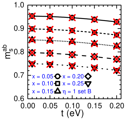
Figure 28: Contributions from electrons in $a/b$ orbitals to spin order parameter $m_{ab}^{s}$ as function of $t$ as calculated by the uHF method (black symbols). Parameters as in Fig. 20. A fit of $m_{ab}^{s}$ to the polaron theory Eq. (44) for doping concentrations $x=5,10,15,20$ and $25$% is marked by red crosses.

By means of the spin-polaron wave function $|\Psi_{1}(\delta_{c})\rangle$ we can evaluate the reduction of the spin and orbital order due to a single polaron (see Eq. (7.4))

$$m_{ab}^{sP} \cong 1+\frac{2\left(t/e_{0}\right)^{2}}{1+\left(t/e_{0}\right)^{2}},$$

$$m_{ab}^{oP} \cong 1+2\delta_{c}+\frac{2\left(t/e_{0}\right)^{2}}{1+\left(t/e_{0}\right)^{2}}.$$ (43)

We note that the potential of the random far defects will modify the excitation energy $e_{0}$. Moreover, the polarity parameter $\delta_{c}$ too is determined by the interplay of the kinetic energy parameter $t$ and the same far-defect random potentials.

The total reduction of spin- and orbital- order associated with $a/b$ electrons is then (Eq.(7.3)):

$$m_{ab}^{s} \cong 1-x\left[1+\frac{2\left(t/e_{0}\right)^{2}}{1+\left(t/e_{0}\right)^{2}}\right],$$

$$m_{ab}^{o} \cong 1-x\left[1+2\delta_{c}+\frac{2\left(t/e_{0}\right)^{2}}{1+\left(t/e_{0}\right)^{2}}\right].$$ (44)

In Fig. 28, we report a least-square fit of the uHF results for the spin order parameter $m_{ab}^{s}$ to the above polaron expression with a single variational parameter, namely the activation energy $e_{0}$. Since the uHF results represent a statistical average over many defect realizations, the resulting activation energy $e_{0}(x)$ characterizes a typical spin-orbital polaron bound state. It is worth noting that $m_{ab}^{s}$ does not depend on the active bond parameter $\delta_{c}$. This is distinct from the orbital order since the motion of the hole on the active bond creates an orbital defect yet no spin defect (see discussion in Sec. VII).

Our results show that even up to a doping concentration of $x=25$%, the reduction of both order parameters is approximately linear, this holds true even when $t=0.2$ eV, i.e., for a typical value of the kinetic energy parameter for the vanadate compounds. It is worth noting that the uHF is able to describe also the interaction between polarons, which appears however irrelevant in the data range shown in Fig. 28. That the independent polaron ansatz works so well for such huge doping concentrations may appear really surprising. On the other hand, one may have expected this given the extreme localization of the defect states we have inferred by exploring the inverse participation number in Sec. VI.

References

- Imada et al. (1998) M. Imada, A. Fujimori, and Y. Tokura, Metal-Insulator Transitions, Rev. Mod. Phys. 70, 1039 (1998).
- Hwang et al. (2012) H. Y. Hwang, Y. Iwasa, M. Kawasaki, B. Keimer, N. Nagaosa, and Y. Tokura, Emergent phenomena at oxide interfaces, Nature Materials 11, 103 (2012).
- Balents (2010) L. Balents, Spin liquids in frustrated magnets, Nature 464, 199 (2010).
- Sachdev and Keimer (2011) S. Sachdev and B. Keimer, Quantum criticality, Physics Today 64, 29 (2011).
- Savary and Balents (2017) L. Savary and L. Balents, Quantum spin liquids: A review, Reports on Progress in Physics 80, 016502 (2017).
- Zhou et al. (2017) Y. Zhou, K. Kanoda, and T.-K. Ng, Quantum spin liquid states, Rev. Mod. Phys. 89, 025003 (2017).
- Lee et al. (2006) P. A. Lee, N. Nagaosa, and X.-G. Wen, Doping a Mott Insulator: Physics of High-Temperature Superconductivity, Rev. Mod. Phys. 78, 17 (2006).
- Alloul et al. (2009) H. Alloul, J. Bobroff, M. Gabay, and P. J. Hirschfeld, Defects in correlated metals and superconductors, Rev. Mod. Phys. 81, 45 (2009).
- Berg et al. (2011) E. Berg, E. Fradkin, S. A. Kivelson, and J. M. Tranquada, Striped Superconductors: how Spin, Charge and Superconducting Orders Intertwine in the Cuprates, New J. Phys 11, 115004 (2011).
- Avella (2014) A. Avella, Composite Operator Method Analysis of the Underdoped Cuprates Puzzle, Advances in Condensed Matter Physics 2014, 515698 (2014).
- Ellman et al. (1989) B. Ellman, H. M. Jaeger, D. P. Katz, T. F. Rosenbaum, A. S. Cooper, and G. P. Espinosa, Transport studies of La2-xSrxCuO4 near the insulator-metal-superconductor transition, Phys. Rev. B 39, 9012 (1989).
- Khaliullin and Horsch (1993) G. Khaliullin and P. Horsch, Doping dependence of long-range magnetic order in the t-J model, Phys. Rev. B 47, 463 (1993).
- Kastner et al. (1998) M. A. Kastner, R. J. Birgeneau, G. Shirane, and Y. Endoh, Magnetic, transport, and optical properties of monolayer copper oxides, Rev. Mod. Phys. 70, 897 (1998).
- Kugel and Khomskii (1982) K. I. Kugel and D. I. Khomskii, The Jahn-Teller Effect and Magnetism: Transition Metal Compounds, Sov. Phys. Usp. 25, 231 (1982).
- Tokura and Nagaosa (2000) Y. Tokura and N. Nagaosa, Orbital Physics in Transition-Metal Oxides, Science 288, 462 (2000).
- Oleś et al. (2005) A. M. Oleś, G. Khaliullin, P. Horsch, and L. F. Feiner, Fingerprints of Spin-Orbital Physics in Cubic Mott Insulators: Magnetic Exchange Interactions and Optical Spectral Weights, Phys. Rev. B 72, 214431 (2005).
- Khaliullin (2005) G. Khaliullin, Orbital Order and Fluctuations in Mott Insulators, Prog. Theor. Phys. Suppl. 160, 155 (2005).
- Horsch (2007) P. Horsch, Orbital Physics in Transition Metal Oxides: Magnetism and Optics, in Handbook of Magnetism and Advanced Magnetic Materials, edited by H. Kronmueller and S. Parkin (Wiley, New York, 2007).
- Oleś (2012) A. M. Oleś, Fingerprints of Spin-Orbital Entanglement in Transition Metal Oxides, J. Phys. Condens. Matter 24, 313201 (2012).
- Kilian and Khaliullin (1999) R. Kilian and G. Khaliullin, Orbital Polarons in the Metal-Insulator Transition of Manganites, Phys. Rev. B 60, 13458 (1999).
- Feiner and Oleś (1999) L. F. Feiner and A. M. Oleś, Electronic Origin of Magnetic and Orbital Ordering in Insulating LaMnO3, Phys. Rev. B 59, 3295 (1999).
- Weisse and Fehske (2004) A. Weisse and H. Fehske, Microscopic Modelling of Doped Manganites, New J. Phys 6, 158 (2004).
- Daghofer et al. (2004) M. Daghofer, A. M. Oleś, and W. von der Linden, Orbital polarons versus itinerant electrons in doped manganites, Phys. Rev. B 70, 184430 (2004).
- Geck et al. (2005) J. Geck, P. Wochner, S. Kiele, R. Klingeler, P. Reutler, A. Revcolevschi, and B. Buchner, Orbital Polaron Lattice Formation in Lightly Doped La1-xSrxMnO3, Phys. Rev. Lett. 95, 236401 (2005).
- Oleś and Khaliullin (2011) A. M. Oleś and G. Khaliullin, Dimensional Crossover and the Magnetic Transition in Electron Doped Manganites, Phys. Rev. B 84, 214414 (2011).
- Snamina and Oleś (1999) M. Snamina and A. M. Oleś, Spin-Orbital Order in the undoped Manganite LaMnO3 at finite Temperature, Phys. Rev. B 59, 3295 (1999).
- Dagotto et al. (2001) E. Dagotto, T. Hotta, and A. Moreo, Colossal Magnetoresistant Materials: The Key Role of Phase Separation, Phys. Rep. 344, 1 (2001).
- Dagotto (2005) E. Dagotto, Open Questions in CMR Manganites, Relevance of Clustered States and Analogies with Other Compounds Including the Cuprates, New J. Phys 7, 67 (2005).
- Tokura (2006) Y. Tokura, Critical Features of Colossal Magnetoresistive Manganites, Rep. Prog. Phys. 69, 797 (2006).
- De Raychaudhury et al. (2007) M. De Raychaudhury, E. Pavarini, and O. K. Andersen, Orbital Fluctuations in the Different Phases of and , Phys. Rev. Lett. 99, 126402 (2007).
- Khaliullin and Maekawa (2000) G. Khaliullin and S. Maekawa, Orbital Liquid in Three-Dimensional Mott Insulator: LaTiO3, Phys. Rev. Lett. 85, 3950 (2000).
- Mochizuki (2002) M. Mochizuki, Spin and orbital states and their phase transitions of the perovskite-type Ti oxides: Weak coupling approach, J. Phys. Soc. Jpn. 71, 2039 (2002).
- Khaliullin and Okamoto (2003) G. Khaliullin and S. Okamoto, Theory of orbital state and spin interactions in ferromagnetic titanates, Phys. Rev. B 68, 205109 (2003).
- Ishihara (2004) S. Ishihara, Orbital wave and its observation in orbital-ordered titanates and vanadates, Phys. Rev. B 69, 075118 (2004).
- Cheng et al. (2008) J.-G. Cheng, Y. Sui, J.-S. Zhou, J. B. Goodenough, and W. H. Su, Transition from Orbital Liquid to Jahn-Teller Insulator in Orthorhombic Perovskites , Phys. Rev. Lett. 101, 087205 (2008).
- Ulrich et al. (2015) C. Ulrich, G. Khaliullin, M. Guennou, H. Roth, T. Lorenz, and B. Keimer, Spin-Orbital Excitation Continuum and Anomalous Electron-Phonon Interaction in the Mott Insulator , Phys. Rev. Lett. 115, 156403 (2015).
- Schooley et al. (1964) J. F. Schooley, W. R. Hosler, and M. L. Cohen, Superconductivity in Semiconducting SrTi, Phys. Rev. Lett. 12, 474 (1964).
- Kozuka et al. (2009) Y. Kozuka, M. Kim, C. Bell, B. G. Kim, Y. Hikita, and H. Y. Hwang, Two-dimensional normal-state quantum oscillations in a superconducting heterostructure, Nature 462, 487 (2009).
- Li et al. (2011) L. Li, C. Richter, J. Mannhart, and R. C. Ashoori, Coexistence of magnetic order and two-dimensional superconductivity at LaAlO3/SrTiO3 interfaces, Nature Phys. 7, 762 (2011).
- Gabay and Triscone (2013) M. Gabay and J. M. Triscone, Hund rules with a twist, Nature Physics 9, 610 (2013).
- Ren et al. (1998) Y. Ren, T. T. M. Palstra, D. I. Khomskii, E. Pellegrin, A. A. Nugroho, A. A. Menovsky, and G. A. Sawatzky, Temperature-induced magnetization reversal in a YVO3 single crystal, Nature 396, 441 (1998).
- Ren et al. (2000) Y. Ren, T. T. M. Palstra, D. I. Khomskii, A. A. Nugroho, A. A. Menovsky, and G. A. Sawatzky, Magnetic properties of YVO3 single crystals, Phys. Rev. B 62, 6577 (2000).
- Khaliullin et al. (2001) G. Khaliullin, P. Horsch, and A. M. Oleś, Spin Order due to Orbital Fluctuations: Cubic Vanadates, Phys. Rev. Lett. 86, 3879 (2001).
- Horsch et al. (2003) P. Horsch, G. Khaliullin, and A. M. Oleś, Dimerization versus Orbital-Moment Ordering in a Mott Insulator YVO3, Phys. Rev. Lett. 91, 257203 (2003).
- Ulrich et al. (2003) C. Ulrich, G. Khaliullin, J. Sirker, M. Reehuis, M. Ohl, S. Miyasaka, Y. Tokura, and B. Keimer, Magnetic Neutron Scattering Study of YVO3: Evidence for an Orbital Peierls State, Phys. Rev. Lett. 91, 257202 (2003).
- Sirker and Khaliullin (2003) J. Sirker and G. Khaliullin, Entropy driven dimerization in a one-dimensional spin-orbital model, Phys. Rev. B 67, 100408 (2003).
- Sirker et al. (2008) J. Sirker, A. Herzog, A. M. Oleś, and P. Horsch, Thermally Activated Peierls Dimerization in Ferromagnetic Spin Chains, Phys. Rev. Lett. 101, 157204 (2008).
- Miyasaka et al. (2003) S. Miyasaka, Y. Okimoto, M. Iwama, and Y. Tokura, Spin-orbital phase diagram of perovskite-type RVO3 (=rare-earth ion or Y), Phys. Rev. B 68, 100406 (2003).
- Miyasaka et al. (2006) S. Miyasaka, J. Fujioka, M. Iwama, Y. Okimoto, and Y. Tokura, Raman study of spin and orbital order and excitations in perovskite-type (, Nd, and Y), Phys. Rev. B 73, 224436 (2006).
- Fujioka et al. (2010) J. Fujioka, T. Yasue, S. Miyasaka, Y. Yamasaki, T. Arima, H. Sagayama, T. Inami, K. Ishii, and Y. Tokura, Critical Competition between two Distinct Orbital-Spin Ordered States in Perovskite Vanadates, Phys. Rev. B 82, 144425 (2010).
- Miyasaka et al. (2007) S. Miyasaka, T. Yasue, J. Fujioka, Y. Yamasaki, Y. Okimoto, R. Kumai, T. Arima, and Y. Tokura, Magnetic Field Switching between the Two Orbital-Ordered States in , Phys. Rev. Lett. 99, 217201 (2007).
- Sage et al. (2007) M. H. Sage, G. R. Blake, C. Marquina, and T. T. M. Palstra, Competing orbital ordering in compounds: High-resolution x-ray diffraction and thermal expansion, Phys. Rev. B 76, 195102 (2007).
- Reehuis et al. (2011) M. Reehuis, C. Ulrich, K. Proke?, S. Mat’a?, J. Fujioka, S. Miyasaka, Y. Tokura, and B. Keimer, Structural and Magnetic Phase Transitions of the Orthovanadates VO3 (=Dy,Ho,Er) as seen via Neutron Diffraction, Phys. Rev. B 83, 064404 (2011).
- Lindfors-Vrejoiu et al. (2017) I. Lindfors-Vrejoiu, L. Jin, C. Himcinschi, J. Engelmayer, F. Hensling, C.-L. Jia, R. Waser, R. Dittmann, and P. H. M. van Loosdrecht, Structure and orbital ordering of ultrathin LaVO3 probed by atomic resolution electron microscopy and Raman spectroscopy, Phys. Status Solidi – Rapid Research Letters 11, 1600350 (2017).
- Miyasaka et al. (2000) S. Miyasaka, T. Okuda, and Y. Tokura, Critical Behavior of Metal-Insulator Transition in La1-xSrxVO3, Phys. Rev. Lett. 85, 5388 (2000).
- Fujioka et al. (2005) J. Fujioka, S. Miyasaka, and Y. Tokura, Orbital disordering and the metal-insulator transition with hole doping in perovskite-type vanadium oxides, Phys. Rev. B 72, 024460 (2005).
- Fujioka et al. (2008) J. Fujioka, S. Miyasaka, and Y. Tokura, Doping Variation of Anisotropic Charge and Orbital Dynamics in Y1-xCaxVO3: Comparison with La1-xSrxVO3, Phys. Rev. B 77, 144402 (2008).
- Reehuis et al. (2016) M. Reehuis, C. Ulrich, P. M. Abdala, P. Pattison, G. Khaliullin, J. Fujioka, S. Miyasaka, Y. Tokura, and B. Keimer, Spin and orbital disordering by hole doping in Pr1-xCaxVO3, Phys. Rev. B 94, 104436 (2016).
- Daghofer et al. (2006) M. Daghofer, P. Horsch, and G. Khaliullin, Magnetic Properties of Spin-Orbital Polarons in Lightly Doped Cobaltates, Phys. Rev. Lett. 96, 216404 (2006).
- Wohlfeld et al. (2009) K. Wohlfeld, A. M. Oleś, and P. Horsch, Orbitally induced string formation in the spin-orbital polarons, Phys. Rev. B 79, 224433 (2009).
- Berciu (2009) M. Berciu, Challenging a Hole to Move through an Ordered Insulator, Physics 2, 55 (2009).
- Bieniasz et al. (2017) K. Bieniasz, M. Berciu, and A. M. Oleś, Orbiton-magnon interplay in the spin-orbital polarons of and , Phys. Rev. B 95, 235153 (2017).
- Avella et al. (2015) A. Avella, A. M. Oleś, and P. Horsch, Defects, Disorder, and Strong Electron Correlations in Orbital Degenerate, Doped Mott Insulators, Phys. Rev. Lett. 115, 206403 (2015).
- Chen et al. (1991) C. Y. Chen, R. J. Birgeneau, M. A. Kastner, N. W. Preyer, and T. Thio, Frequency and magnetic-field dependence of the dielectric constant and conductivity of , Phys. Rev. B 43, 392 (1991).
- Chen et al. (2009) W. Chen, G. Khaliullin, and O. P. Sushkov, Coulomb disorder effects on angle-resolved photoemission and nuclear quadrupole resonance spectra in cuprates, Phys. Rev. B 80, 094519 (2009).
- Horsch et al. (2008) P. Horsch, A. M. Oleś, L. F. Feiner, and G. Khaliullin, Evolution of Spin-Orbital-Lattice Coupling in the VO3 Perovskites, Phys. Rev. Lett. 100, 167205 (2008).
- Horsch and Oleś (2011) P. Horsch and A. M. Oleś, Defect States and Spin-Orbital Physics in Doped Vanadates Y1-xCaxVO3, Phys. Rev. B 84, 064429 (2011).
- Bizen et al. (2012) D. Bizen, H. Nakao, K. Iwasa, Y. Murakami, T. Osakabe, J. Fujioka, T. Yasue, S. Miyasaka, and Y. Tokura, Magnetic Phase Diagrams of YVO3 and TbVO3 under High Pressure, J. Phys. Soc. Jpn 81, 024715 (2012).
- Maiti et al. (1998) K. Maiti, P. Mahadevan, and D. D. Sarma, Evolution of Spectral Function in a Doped Mott Insulator: Surface vs Bulk Contributions, Phys. Rev. Lett. 80, 2885 (1998).
- Maiti and Sarma (2000) K. Maiti and D. D. Sarma, Spectroscopic investigations of the electronic structure and metal-insulator transitions in a Mott-Hubbard system La1-xCaxVO3, Phys. Rev. B 61, 2525 (2000).
- Pen et al. (1999) H. F. Pen, M. Abbate, A. Fuijmori, Y. Tokura, H. Eisaki, S. Uchida, and G. A. Sawatzky, Electronic structure of studied by high-energy spectroscopies, Phys. Rev. B 59, 7422 (1999).
- Gantmakher (2005) V. F. Gantmakher, Electrons and Disorder in Solids (Clarendon Press, Oxford, 2005).
- Drabold and Estreicher (2007) D. A. Drabold and S. K. Estreicher, eds., Theory of Defects in Semiconductors (Springer, Berlin Heidelberg, 2007).
- Anderson (1958) P. W. Anderson, Absence of Diffusion in Certain Random Lattices, Phys. Rev 109, 1492 (1958).
- Lee and Ramakrishnan (1985) P. A. Lee and T. V. Ramakrishnan, Disordered electronic systems, Rev. Mod. Phys. 57, 287 (1985).
- Altshuler and Aronov (1979) B. L. Altshuler and A. A. Aronov, Zero bias anomaly in tunnel resistance and electron-electron interaction, Solid State Commun. 30, 115 (1979).
- Pollack (1970) M. Pollack, Effect of carrier-carrier interactions on some transport properties in disordered semiconductors, Discuss. Faraday Soc. 50, 20 (1970).
- Efros and Shklovskii (1975) A. L. Efros and B. I. Shklovskii, Coulomb gap and low temperature conductivity of disordered systems, J. Phys. C 8, L49 (1975).
- Efros (1976) A. L. Efros, Coulomb gap in disordered systems, J. Phys. C 9, 2021 (1976).
- Efros et al. (2011) A. L. Efros, B. Skinner, and B. I. Shklovskii, Coulomb gap in the one-particle density of states in three-dimensional systems with localized electrons, Phys. Rev. B 84, 064204 (2011).
- Shinaoka and Imada (2009) H. Shinaoka and M. Imada, Single-particle excitations under coexisting electron correlation and disorder: a numerical study of the Anderson-Hubbard model, J. Phys. Soc. Jpn 78, 094708 (2009).
- Shinaoka and Imada (2010) H. Shinaoka and M. Imada, Theory of electron transport near Anderson-Mott transition, J. Phys. Soc. Jpn 79, 113703 (2010).
- Epperlein et al. (1997) F. Epperlein, M. Schreiber, and T. Vojta, Quantum Coulomb glass within a Hartree-Fock approximation, Phys. Rev. B 56, 5890 (1997).
- Song et al. (2009) Y. Song, S. Bulut, R. Wortis, and W. A. Atkinson, Effects of strong correlations on the disorder-induced zero-bias anomaly in the extended Anderson–Hubbard model, Journal of Physics: Condensed Matter 21, 385601 (2009).
- Mizokawa et al. (2000) T. Mizokawa, D. I. Khomskii, and G. A. Sawatzky, Charge and orbital ordering in underdoped , Phys. Rev. B 61, R3776 (2000).
- Barreteau et al. (2000) C. Barreteau, R. Guirado-Lopez, D. Spanjaard, M. C. Desjonqueres, and A. M. Oleś, spd tight-binding model of magnetism in transition metals: Application to Rh and Pd clusters and slabs, Phys. Rev. B 61, 7781 (2000).
- Schickling et al. (2011a) T. Schickling, F. Gebhard, and J. Bonemann, Antiferromagnetic Order in Multiband Hubbard Models for Iron Pnictides, Phys. Rev. Lett. 106, 146402 (2011a).
- Solovyev (2008) V. I. Solovyev, Combining DFT and many-body methods to understand correlated materials, J. Phys. Condens. Matter 20, 293201 (2008).
- Carrasco et al. (2006) J. Carrasco, F. Illas, N. Lopez, E. A. Kotomin, Y. F. Zhukovskii, R. A. Evarestov, Y. A. Mastrikov, S. Piskunov, and J. Maier, First-principles calculations of the atomic and electronic structure of F centers in the bulk and on the (001) surface of SrTiO3, Phys. Rev. B 73, 064106 (2006).
- Pavlenko et al. (2012) N. Pavlenko, T. Kopp, E. Y. Tsymbal, J. Mannhart, and G. A. Sawatzky, Oxygen vacancies at titanate interfaces: Two-dimensional magnetism and orbital reconstruction, Phys. Rev. B 86, 064431 (2012).
- Avella et al. (2013) A. Avella, P. Horsch, and A. M. Oleś, Defect States and Excitations in a Mott Insulator with Orbital Degrees of Freedom: Mott-Hubbard Gap versus Optical and Transport Gaps in Doped Systems, Phys. Rev. B 87, 045132 (2013).
- Mizokawa and Fujimori (1995) T. Mizokawa and A. Fujimori, Unrestricted Hartree-Fock study of transition-metal oxides: Spin and orbital ordering in perovskite-type lattice, Phys. Rev. B 51, 12880 (1995).
- Mizokawa and Fujimori (1997) T. Mizokawa and A. Fujimori, Hartree-Fock study of charge-ordered states in La2-xSrxCuO4 and La2-xSrxNiO4, Phys. Rev. B 56, 11920 (1997).
- Weng and Terakura (2010) H. Weng and K. Terakura, Phase diagram of LaVO3 under epitaxial strain: Implications for thin films grown on SrTiO3 and LaAlO3 substrates, Phys. Rev. B 82, 115105 (2010).
- Solovyev (2009) V. I. Solovyev, Long-Range Magnetic Interactions Induced by the Lattice Distortions and the Origin of the E-Type Antiferromagnetic Phase in the Undoped Orthorhombic Manganites, J. Phys. Soc. Jpn. 78, 054710 (2009).
- Kubo and Thalmeier (2009) K. Kubo and P. Thalmeier, Multiorbital Effects on Antiferromagnetism in Fe Pnictides, J. Phys. Soc. Jpn. 78, 083704 (2009).
- Schickling et al. (2011b) T. Schickling, F. Gebhard, and J. Bünemann, Antiferromagnetic Order in Multiband Hubbard Models for Iron Pnictides, Phys. Rev. Lett. 106, 146402 (2011b).
- Luo et al. (2013) Q. Luo, A. Nicholson, J. Rincón, S. Liang, J. Riera, G. Alvarez, L. Wang, W. Ku, G. D. Samolyuk, A. Moreo, and E. Dagotto, Magnetic states of the two-leg-ladder alkali metal iron selenides Fe2Se3, Phys. Rev. B 87, 024404 (2013).
- Luo and Dagotto (2014) Q. Luo and E. Dagotto, Magnetic phase diagram of a five-orbital Hubbard model in the real-space Hartree-Fock approximation varying the electronic density, Phys. Rev. B 89, 045115 (2014).
- Bell and Dean (1970) R. J. Bell and P. Dean, Atomic vibrations in vitreous silica, Discussions of the Faraday Society 50, 55 (1970).
- Thouless (1974) D. J. Thouless, Electrons in disordered systems and the theory of localization, Phys. Rep 13, 93 (1974).
- Wegner (1980) F. Wegner, Inverse participation ratio in 2+ dimensions, Z. Physik B 36, 209 (1980).
- Nguyen and Goodenough (1995) H. C. Nguyen and J. B. Goodenough, Localized-itinerant electronic transition in the perovskite system La1-xCaxVO3, Phys. Rev. B 52, 8776 (1995).
- Damascelli et al. (2003) A. Damascelli, Z. Hussain, and Z.-X. Shen, Angle-resolved photoemission studies of the cuprate superconductors, Rev. Mod. Phys. 75, 473 (2003).
- Comin and Damascelli (2016) R. Comin and A. Damascelli, Resonant X-Ray Scattering Studies of charge order in cuprates, Annu. Rev. Condens. Matter Phys. 7, 369 (2016).
- Khaliullin et al. (2004) G. Khaliullin, P. Horsch, and A. M. Oleś, Theory of Optical Spectral Weights in Mott Insulators with Orbital Degrees of Freedom, Phys. Rev. B 70, 195103 (2004).
- Tsvetkov et al. (2004) A. A. Tsvetkov, F. P. Mena, P. H. M. van Loosdrecht, D. van der Marel, Y. Ren, A. A. Nugroho, A. A. Menovsky, I. S. Elfimov, and G. A. Sawatzky, Structural, electronic, and magneto-optical properties of YVO3, Phys. Rev. B 69, 075110 (2004).
- Harris et al. (2003) A. B. Harris, T. Yildirim, A. Aharony, O. Entin-Wohlman, and I. Y. Korenblit, Unusual Symmetries in the Kugel-Khomskii Hamiltonian, Phys. Rev. Lett. 91, 087206 (2003).
- Daghofer et al. (2008) M. Daghofer, K. Wohlfeld, A. M. Oleś, E. Arrigoni, and P. Horsch, Absence of Hole Confinement in Transition-Metal Oxides with Orbital Degeneracy, Phys. Rev. Lett. 100, 066403 (2008).
- Li (2015) Y. Li, Exact results for itinerant ferromagnetism in a -orbital system on cubic and square lattices, Phys. Rev. B 91, 115122 (2015).
- Oleś (1983) A. M. Oleś, Antiferromagnetism and Correlation of Electrons in Transition Metals, Phys. Rev. B 28, 327 (1983).
- Daghofer et al. (2010) M. Daghofer, A. Nicholson, A. Moreo, and E. Dagotto, Three orbital model for the iron-based superconductors, Phys. Rev. B 81, 014511 (2010).
- Mayr and Horsch (2006) M. Mayr and P. Horsch, Domain-wall excitations and optical conductivity in one-dimensional Wigner lattices, Phys. Rev. B 73, 195103 (2006).
- Matiks et al. (2009) Y. Matiks, P. Horsch, R. K. Kremer, B. Keimer, and A. V. Boris, Exciton Doublet in the Mott-Hubbard Insulator Identified by Spectral Ellipsometry, Phys. Rev. Lett. 103, 187401 (2009).
- Brinkman and Rice (1970) W. F. Brinkman and T. M. Rice, Single-Particle Excitations in Magnetic Insulators, Phys. Rev. B 2, 1324 (1970).
- Eskes et al. (1991) H. Eskes, M. B. J. Meinders, and G. A. Sawatzky, Anomalous transfer of spectral weight in doped strongly correlated systems, Phys. Rev. Lett. 67, 1035 (1991).
- Meinders et al. (1993) M. B. J. Meinders, H. Eskes, and G. A. Sawatzky, Spectral-weight transfer: Breakdown of low-energy-scale sum rules in correlated systems, Phys. Rev. B 48, 3916 (1993).
- Fujimori et al. (1992) A. Fujimori, I. Hase, H. Namatame, Y. Fujishima, Y. Tokura, H. Eisaki, S. Uchida, K. Takegahara, and F. M. F. de Groot, Evolution of the spectral function in Mott-Hubbard systems with configuration, Phys. Rev. Lett. 69, 1796 (1992).
- Dagotto et al. (1992) E. Dagotto, A. Moreo, F. Ortolani, D. Poilblanc, and J. Riera, Static and dynamical properties of doped Hubbard clusters, Phys. Rev. B 45, 10741 (1992).
- Eskes and Oleś (1994) H. Eskes and A. M. Oleś, Two Hubbard Bands: Weight Transfer in Optical and One-Particle Spectra, Phys. Rev. Lett. 73, 1279 (1994).
- Eskes et al. (1994) H. Eskes, A. M. Oleś, M. B. J. Meinders, and W. Stephan, Spectral properties of the Hubbard bands, Phys. Rev 50, 17980 (1994).
- de’Medici et al. (2005) L. de’Medici, A. Georges, and S. Biermann, Orbital-selective Mott transition in multiband systems: Slave-spin representation and dynamical mean-field theory, Phys. Rev. B 72, 205124 (2005).
- Vaugier et al. (2012) L. Vaugier, H. Jiang, and S. Biermann, Hubbard and Hund exchange in transition metal oxides: Screening versus localization trends from constrained random phase approximation, Phys. Rev. B 86, 165105 (2012).
- Vollhardt (1997) D. Vollhardt, Characteristic Crossing Points in Specific Heat Curves of Correlated Systems, Phys. Rev. Lett. 78, 1307 (1997).
- Greger et al. (2013) M. Greger, M. Kollar, and D. Vollhardt, Isosbestic points: How a narrow crossing region of curves determines their leading parameter dependence, Phys. Rev. B 87, 195140 (2013).
- Guhr et al. (1998) T. Guhr, A. Muller-Groeling, and H. A. Weidenmuller, Random-matrix theories in quantum physics: Common concepts, Phys. Rep. 299, 190 (1998).
- Ono et al. (1989) Y. Ono, T. Ohtsuki, and B. Kramer, Inverse Participation Number and Fractal Dimensionality of Electronic States in a Two Dimensional System in Strong Perpendicular Magnetic Field, J. Phys. Soc. Jpn. 58, 1705 (1989).
- Evers and Mirlin (2008) F. Evers and A. D. Mirlin, Anderson transitions, Rev. Mod. Phys. 80, 1355 (2008).
- Misguich et al. (2016) G. Misguich, V. Pasquier, and J.-M. Luck, Inverse participation ratios in the XXZ spin chain, Phys. Rev. B 94, 155110 (2016).
- Luitz et al. (2015) D. J. Luitz, N. Laflorencie, and F. Alet, Many-body localization edge in the random-field Heisenberg chain, Phys. Rev. B 91, 081103 (2015).
- Mott (1974) N. F. Mott, Metal-Insulator Transition (Taylor and Francis, London, 1974).
- Braganca et al. (2015) H. Braganca, M. C. O. Aguiar, J. Vucicević, D. Tanasković, and V. Dobrosavljević, Anderson localization effects near the Mott metal-insulator transition, Phys. Rev. B 92, 125143 (2015).
- Martinez and Horsch (1991) G. Martinez and P. Horsch, Spin polarons in the t-J model, Phys. Rev. B 44, 317 (1991).
- Wróbel et al. (2008) P. Wróbel, W. Suleja, and R. Eder, Spin-polaron band structure and hole pockets in underdoped cuprates, Phys. Rev. B 78, 064501 (2008).
- Wohlfeld et al. (2008) K. Wohlfeld, M. Daghofer, A. M. Oleś, and P. Horsch, Spectral properties of orbital polarons in Mott insulators, Phys. Rev. B 78, 214423 (2008).
- Wróbel and Oleś (2010) P. Wróbel and A. M. Oleś, Ferro-Orbitally Ordered Stripes in Systems with Alternating Orbital Order, Phys. Rev. Lett. 104, 206401 (2010).
- Bała and Horsch (2005) J. Bała and P. Horsch, Spin-orbital physics in the optical conductivity of quarter-filled manganites, Phys. Rev. B 72, 012404 (2005).
- Wróbel et al. (2012) P. Wróbel, R. Eder, and A. M. Oleś, Optical conductivity due to orbital polarons in systems with orbital degeneracy, Phys. Rev. B 86, 064415 (2012).
- van den Brink et al. (2000) J. van den Brink, P. Horsch, and A. M. Oleś, Photoemission Spectra of Controlled by Orbital Excitations, Phys. Rev. Lett. 85, 5174 (2000).
- Brzezicki et al. (2014) W. Brzezicki, M. Daghofer, and A. M. Oleś, Mechanism of hole propagation in the orbital compass models, Phys. Rev. B 89, 024417 (2014).
- Bieniasz et al. (2016) K. Bieniasz, M. Berciu, M. Daghofer, and A. M. Oleś, Green’s function variational approach to orbital polarons in KCuF3, Phys. Rev. B 94, 085117 (2016).
- Zaanen and Oleś (1993) J. Zaanen and A. M. Oleś, Carriers binding to excitons: Crystal-field excitations in doped Mott-Hubbard insulators, Phys. Rev. B 48, 7197 (1993).
- Kim et al. (2002) M. W. Kim, J. H. Jung, K. H. Kim, H. J. Lee, J. Yu, T. W. Noh, and Y. Moritomo, Spin-Orbital Pattern Dependent Polaron Absorption in Manganites, Phys. Rev. Lett. 89, 016403 (2002).
- Yamauchi and Picozzi (2013) K. Yamauchi and S. Picozzi, Mechanism of Ferroelectricity in Half-Doped Manganites with Pseudocubic and Bilayer Structure, J. Phys. Soc. Jpn 82, 113703 (2013).
- Dougier and Hagenmuller (1975) Dougier and Hagenmuller, Evolution des proprietes cristallographiques, electriques et magnetiques au sein du systeme La1-xSrxVO3 , J. Sol. State Chem. 15, 158 (1975).
- Mott (1989) N. F. Mott, Doped antiferromagnetic insulators : a model for high temperature superconductivity, J. Phys. France 50, 2811 (1989).
- Horsch and von der Linden (1988) P. Horsch and W. von der Linden, On dielectric response and quasiparticles in semiconductors and insulators, Physica Scripta 38, 613 (1988).
- Pollak (2012) M. Pollak, Extension of Anderson’s Localization Theory to Interacting Systems, Journal of Physics: Conference Series 376, 012012 (2012).