Asymptotic enumeration of perfect matchings in $m$-barrel fullerene graphs

Abstract

A connected planar cubic graph is called an $m$-barrel fullerene and denoted by $F(m,k)$, if it has the following structure: The first circle is an $m$-gon. Then $m$-gon is bounded by $m$ pentagons. After that we have additional k layers of hexagons. At the last circle $m$-pentagons connected to the second $m$-gon. In this paper we asymptotically count by two different methods the number of perfect matchings in $m$-barrel fullerene graphs, as the number of hexagonal layers is large, and show that the results are equal.

2010 Mathematics Subject Classification. 05C30, 05C70, 15A15.

Keywords. perfect matchings, fullerene graph, m-barrel fullerene

1 Introduction

A fullerene graph is a cubic, planar, 3-connected graph with only pentagonal and hexagonal faces. It follows easily from the Euler’s formula that there must be exactly 12 pentagonal faces, while the number of hexagonal faces can be zero or any natural number greater than one. The smallest possible fullerene graph is the dodecahedron on 20 vertices, while the existence of fullerene graphs on an even number of vertices greater than 22 follows from a result by Grünbaum and Motzkin [Grünbaum and Motzkin(1963)]. Classical fullerene graphs have been intensely researched since the discovery of buckminsterfullerene in the fundamental paper [Kroto et al.(1985)Kroto, Heath, Obrien, Curl, and Smalley], which appeared in 1985, and gave rise to the whole new area of fullerene science.

A connected $3$-regular planar graph $G=(V,E)$ is called an $m$-generalized fullerene if exactly two of its faces are $m$-gons and all other faces are pentagons and/or hexagons. (We also count the outer (unbounded) face of $G$.) In the rest of the paper we only consider $m\geq 3$; note that for $m=5,6$ an $m$-generalized fullerene graph is a classical fullerene graph. As for the classical fullerenes it is easy to show that the number of pentagons is fixed, while the number of hexagons is not determined. The smallest $m$-generalized fullerene has $4m$ vertices and no hexagonal faces. By inserting $k\geq 0$ layers of $m$ hexagons between two layers of pentagons we reach the symmetric class of m-generalized fullerenes called $m$-barrel fullerenes.

The $m$-barrel fullerene with $k$ layers of hexagons, denoted by $F(m,k)$, can be defined as a sequence of concentric layers as follows: the first circle is an $m$-gon. This $m$-gon is bounded by $m$ pentagons. After that we have additional $k$ layers of $m$ of hexagon. Then one again has a circular layer with $m$-pentagons connected to the second $m$-gon, represented by the outer face. $m$-barrell fullerenes can be neatly represented graphically using a sequence of $k+3$ concentric circles with monotonically increasing radii such that the innermost and the outermost circle each have $m$ vertices (representing, hence, two $m$-gons), while all other circles have $2m$ vertices each, connecting alternatively to vertices of the larger or smaller circle to create hexagonal an pentagonal faces. An example is shown in Figure 1.

Figure 1: The $m$-barrel fullerene $F(8,2)$.

The $m$-barrel fullerenes are the main subjects of the present paper, since their highly symmetric structure allows for obtaining good bounds and even exact results on their quantitative graph properties. For example Kutnar and Marušič in [Kutnar and Marušič(2008)] studied Hamiltonicity and cyclic edge-conectivity of $F(5,k)$. See also [Behmaram et al.(2016)Behmaram, Došlić, and Friedland] for some structural results about $m$-barrel fullerene graphs, such as the diameter, Hamiltonicity and the leapfrog transformation.

A matching $M$ in a graph $G$ is a collection of edges of $G$ such that no two edges of $M$ share a vertex. If every vertex of $G$ is incident to an edge of $M$, the matching $M$ is said to be perfect. A perfect matching is also often called a dimer configuration in mathematical physics and chemestry. Perfect matchings have played an important role in the chemical graph theory, in particular for benzenoid graphs, where their number correlates with the compound’s stability. Although it turned out that for fullerenes they do not have the same role as for benzenoids, there are many results concerning their structural and enumerative properties. See [Behmaram and Friedland(2013), Andova et al.(2012)Andova, Došlić, Krnc, Lužar, and Škrekovski, Došlić(2008), Došlić(2009), Kardoš et al.(2009)Kardoš, Král’, Miškuf, and Sereni] for more result on perfect matchings in fullerenes. We denote by $\Phi(G)$ the number of perfect matchings of $G$.

The goal of this paper is to compute the growth constant $\rho(m)$ for the number of perfect matchings for the family of graphs $F(m,k)$ for a fixed $m$, as $k$ goes to infinity:

$$\rho(m)=\lim_{k\to\infty}\Phi(F(m,k))^{1/k}.$$ (1.1)

Behmaram, Doslic and Friedland in [Behmaram et al.(2016)Behmaram, Došlić, and Friedland] obtained some exact results for the number of perfect matching for the values of $m\leq 5$, using the transfer matrix method, described in Section 3, allowing in particular for a direct computation of the growth $\rho(m)$ for $m\in\{3,4,5\}$, see Theorem 3.1.

In this paper, we estimate the number of perfect matchings of $F(m,k)$ for large $k$, and compute exactly $\rho(m)$ for any $m$.

Theorem 1.1.

Let $m\geq 3$. The growth constant for the family of $m$-barrel fullerenes is equal to

$$\rho(m)=\prod_{j=1}^{\lfloor\frac{m+1}{3}\rfloor}\left(2\cos\frac{\pi(2j-1)}{m}\right)^{2}.$$

We propose two proofs using two different methods from combinatorics:

• the transfer matrix approach (Section 3), which is explicitly diagonalized using (a baby version) of the Bethe Ansatz [Bethe(1931)], method from integrable systems to diagonalize the Hamiltonian of integrable spin chains for example;

• an approach using coding with non-intersecting paths, counted by determinants via the Lindström-Gessel-Viennot lemma.

These two approaches are classical in some branches of combinatorics, and believe that they can be of great use to study properties of fullerene graphs, especially those with some symmetry.

Before we introduce these methods, we apply some transformations to the graph $F(m,k)$ to see it as piece of the hexagonal lattice wrapped on the cyclinder, with specific boundaray conditions, in order to finally reformulate the question of perfect matchings on $F(m,k)$ as a problem of tilings with rhombi.

2 Perfect matchings on $m$-barrel fullerenes and tilings of cylinders with rhombi

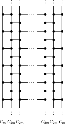
Figure 2: Left: an $m$-barrel fullerene, represented on the cylinder. The top and bottom are identified to create the cylinder. The cycles $C_{m}$ on the extremities are the boundary of the cylinder and correspond to the boundaries of the $m$-gons in the representation of Figure 1. Right: the same graph on the cylinder, slightly deformed so that hexagonal faces are regular.

To begin with, instead of presenting the graph on the sphere, as on Figure 1, we draw it on the cylinder, where now the $m$-gons represent the two components of the boundary of this cylinder. These two cycles of size $m$ are separated by $k+1$ cycles of size $2m$ winding around the cylinder, each of them connected to their left and right neighboring cycle by $m$ horizontal edges to create the pentagonal/hexagonal faces, arranged in a brickwall pattern on the cylinder. See Figure 2 (left). This brickwall pattern can in turn be deformed so that the hexagonal faces are now regular polygonal, so that the bulk of the graph looks like the regular honeycomb lattice wrapped on a cylinder. See Figure 2 (right).

It is obvious that perfect matchings such a hexagonal graph on the cylinder with pentagonal faces on the boundary are in bijection with tilings of the cylinder with unit rhombi, where some of the rhombi are allowed to stick out of the boundary. See Figure 3.

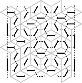
Figure 3: The correspondence between perfect matchings on $F(6,5)$ (left) and rhombi tiling on the cylinder. Recall that the graph is drawn on a cylinder, so that the edges at the top are connected to vertices at the bottom.

In the sequel, we will use indifferently the language of perfect matchings and tilings with rhombi. In particular horizontal edges in a perfect matching of $F(m,k)$ correspond exactly to horizontal rhombi in the tiling picture. Note that as long as there is at least a horizontal rhombus in the tiling, the position of all horizontal rhombi is sufficient to reconstruct the whole tiling. On the other hand, the two other types of rhombi (with vertical edges) form non-interesecting paths connecting the left and right boundaries. The collection of these paths also characterize the whole tiling.

In the next two sections, we present two methods to count the number of perfect matchings of $F(m,k)$: the transfer matrix method, which uses the horizontal rhombi, and a method using the collection of non-intersecting paths.

3 The transfer matrix method

The first method we present, using a transfer matrix, is well suited to count the number of perfect matchings on graphs with some regularity or periodicity, which is indeed the case here.

Before introducing the transfer matrix, we need to fix some notation. For $j\in\{1,..,k\}$, denote by $E_{j}$ the subset of horizontal edges of $F(m,k)$ between the $j$th and the $(j+1)$th cycle $C_{2m}$. Extend this definition to $E_{0}$ (resp. $E_{k+1}$) to be the subset of horizontal edges before the first (resp. after the last) cycle $C_{2m}$, which come from the pentagons at the left (resp. right) end.

Figure 4: Labeling of the horizontal edges of $F(m,k)$.

We label the edges of $E_{j}$ by $e_{j,l}$, $l\in\{0,\dots,m-1\}$. Indices $l$ increase when going “up”, and they should be thought modulo $m$, so that $e_{j,l+m}$ is the same as $e_{j,l}$. For consistency of the labeling between different layers of horizontal edges, we take the convention that $e_{j,l}$ has on its left $e_{j-1,l}$ just below and $e_{j-1,l+1}$ just above. See Figure 4. Subsets of $E_{j}$ are thus in bijection of subsets of $I_{m}=\{0,\dots,m-1\}$.

Given two subsets $S_{j-1}$ and $S_{j}$ of respectively $E_{j-1}$ and $E_{j}$, let $a_{j}(S_{j-1},S_{j1})$ be the number of perfect matchings of the $j$-th cycle where we removed vertices attached to the edges in $S_{j-1}\cup S_{j}$. Because of invariance by translation, this number does not really depend on $j$, but only on the subsets $S,T\subset I_{m}$ in bijection with $S_{j-1}$ and $S_{j}$ respectively. We store all these numbers in a matrix $A=(a_{S,T})_{S,T\subset I_{m}}$. This matrix $A$ (which implicitly depends on $m$) is called the transfer matrix of the model.

It will be convenient to use the bra and ket notation from quantum mechanics. The matrix $A$ is thought as the matrix of a linear operator on a vector space in the orthonormal basis $(|T\rangle)_{T\subset I_{m}}$ of some vector space of dimension $2^{m}$, indexed by subsets of $I_{m}$.

The dual basis $(\langle S|)_{S\subset I_{m}}$ satisfies that for all $S,T\subset I_{m}$,

$$\langle S|T\rangle=\begin{cases}1&\text{if $S=T$,}\\ 0&\text{otherwise.}\end{cases}$$

With these notations, we have $A=\sum_{S,T}a_{S,T}|S\rangle\langle T|$ and $a_{S,T}=\langle S|A|T\rangle$.

Let us make a few remarks on this matrix $A$:

• $A$ is invariant by “vertical translation”.

• because of the left/right and top/bottom symmetry, we have $\langle S|A|T\rangle=\langle T|A|S\rangle$: in this basis, $A$ is symmetric, thus diagonalisable, with orthogonal eigenspaces.

• Due to geometric constraints of the problem, two sets $S_{j-1}$ and $S_{j}$ coming from a perfect matching should interlace. In particular if $|S|\neq|T|$, $\langle S|A|T\rangle=0$. If we write down the matrix, with subsets indexing rows and columns ordered according to their cardinal, then $A$ has a block diagonal structure.

• Perron-Frobenius theorem guarantees, that on each block, the largest eigenvalue is non-degerate, and associated with an eigenvector wich can be chosen with all its entries in that block to be positive.

In this vector space, one can also define a boundary vector $|\Omega\rangle$, corresponding to a formal linear combination of possible configurations coming from possible perfect matchings of $F(m,k)$. Then it is a simple observation that the number of perfect matchings $\Phi(F(m,k))$ of $F(m,k)$ can be expressed with $A$ and $|\Omega\rangle$ as follows

$$\Phi(F(m,k))=\langle\Omega|A^{k+1}|\Omega\rangle,$$ (3.1)

as there are $k+1$ transitions between $E_{j-1}$ and $E_{j}$, for $1\leq j\leq k+1$, each of of them being encoded by a matrix $A$.

Computing explicitly the reduced form of $A$ for $m=3,4$ and $5$, the authors of [Behmaram et al.(2016)Behmaram, Došlić, and Friedland] gave an exact formula for $\Phi(F(3,k)$, $\Phi(F(4,k)$, and $\Phi(F(5,k)$:

Theorem 3.1 ([Behmaram et al.(2016)Behmaram, Došlić, and Friedland]).

let $\Phi(F(m,k))$ denote the number of perfect matching in $F(m,k)$ then for m=3,4,5 we have:

$$\Phi(F(3,k)) =3^{k+2}+1,$$

$$\Phi(F(4,k)) =2(2+\sqrt{2})^{k+1}+2(2-\sqrt{2})^{k+1}+2^{k+3}+1,$$

$$\Phi(F(5,k)) =5^{k+2}+5\left[\left(\frac{5+\sqrt{5}}{2}\right)^{k}+\left(\frac{5-\sqrt{5}}{2}\right)^{k}\right]+1.$$

3.1 The Bethe Ansatz

It turns out that it is possible to express the eigenvalues (and eigenvectors) of $A$ for any value of $m$, using the so-called Bethe Ansatz [Bethe(1931)], a method used in theoretical physics to diagonalize the Hamiltonian of integrable systems with interaction, by looking for eigenvectors as a superposition of plane waves.

In our problem, the situation is particularly simple: it turns out, as we will see later, that all the eigenvectors are expressed in terms of determinants (Slater determinants in quantum mechanics terminology). This is a feature of the dimer model and its free-fermionic nature.

As mentioned above, $A$ has a block diagonal structure. The blocks (or sectors) are indexed by $p\in\{0,\dots,m\}$, the number of elements of the corresponding subsets indexing rows and columns. The block indexed with $p$ has size $\binom{m}{p}$.

For any $p$, we look for $\binom{m}{p}$ eigenvectors as linear combination of basis vectors $|S\rangle$, where $|S|=p$.

For the counting problem we are interested in, the structure of eigenvectors and eigenvalues is a bit degenerated. In order to perform the computations, it is easier to introduce a weighted version of the transition matrix: Fix $b$, and $c$ positive, distinct real numbers, and put weight $b$ (resp. $c$) on every upgoing (downgoing) edge from left to right. let $B=(\langle S|B|T\rangle)$ be the matrix such that $\langle S|B|T\rangle$ is the sum of all perfect matchings on a layer with boundary conditions described by $S$ and $T$: if $S$ and $T$ are empty, then $\langle S|B|T\rangle=b^{m}+c^{m}$. If $S$ and $T$ are not empty and compatible, then there is only one perfect matching for the transition from $S$ to $T$ and $\langle S|B|T\rangle$ is of the form $b^{j}c^{m-j-|S|}$ for some $j$.

3.2 The $p=0$ and $p=1$ sectors

The sector $p=0$ is one-dimensional, and spanned by $\emptyset$. If we don’t remove any vertices, the cycle of length $2m$ has 2 perfect matchings, consisting of odd and even edges respectively. Therefore, we have

$$B|\emptyset\rangle=(b^{m}+c^{m})|\emptyset\rangle.$$

The sector $p=1$ is $m$-dimensional. For $l=0,\dots,m-1$, if $S=\{l\}$, we note simply $|l\rangle$ for $|S\rangle$.

We have:

$$B|l\rangle=\sum_{l^{\prime}=0}^{l}c^{l-l^{\prime}}b^{m-1+l^{\prime}-l}|l^{\prime}\rangle+\sum_{l^{\prime}=l+1}^{m-1}b^{l^{\prime}-l-1}c^{m+l-l^{\prime}}|l^{\prime}\rangle.$$

For $z\in\mathbb{C}^{*}$, we define the vector

$$|z\rangle=\sum_{l}z^{l}|l\rangle.$$

Let us compute the action of $B$ on $|z\rangle$, by exchanging the sums over $l$ and $l^{\prime}$:

$$B|z\rangle =\sum_{l^{\prime}=0}^{m-1}\left(\sum_{l=l^{\prime}}^{m-1}b^{m+l^{\prime}-1-l}c^{l-l^{\prime}}z^{l}+\sum_{l=0}^{l^{\prime}-1}b^{l^{\prime}-1-l}c^{m-l^{\prime}+l}z^{l}\right)|l^{\prime}\rangle$$

$$=\sum_{l^{\prime}=0}^{m-1}\left(b^{m+l^{\prime}}c^{-l^{\prime}}\frac{(cz/b)^{m}-(cz/b)^{l^{\prime}}}{cz-b}+b^{l^{\prime}}c^{m-l^{\prime}}\frac{(cz/b)^{l^{\prime}}-1}{cz-b}\right)|l^{\prime}\rangle$$

$$=\sum_{l^{\prime}=0}^{m-1}\frac{c^{m}-b^{m}}{cz-b}z^{l^{\prime}}|l^{\prime}\rangle+\frac{z^{m}-1}{cz-b}\sum_{l^{\prime}=0}^{m-1}b^{l^{\prime}}c^{m-l^{\prime}}|l^{\prime}\rangle$$

The first term is exactly $\frac{c^{m}-b^{m}}{cz-b}|z\rangle$. If we choose $z$ to be a $m$th root of unity, then the factor in front of the second sum vanishes. Then $|z\rangle$ (which is also an eigenvector of the translation operator) is an eigenvector of $B$, with eigenvalue $\frac{c^{m}-b^{m}}{cz-b}$. The eigenvalues are all distinct for $b\neq c$, and $z=z_{r}=\exp\bigl{(}\frac{2ir\pi}{m}\bigr{)}$, with $r=0,\dots,m-1$

These give $m=\binom{m}{1}$ orthogonal eigenvectors, and the one associated to the largest eigenvalue $\frac{c^{m}-b^{m}}{c-b}$ corresponds to $z=1$ and has all its entries equal.

3.3 The $p=2$ sector

If $S=\{l_{1},l_{2}\}$, with $0\leq l_{1}<l_{2}\leq m-1$, we write $|l_{1},l_{2}\rangle$ instead of $|S\rangle$. Let us write explicitly the action of $B$ on such a vector.

As for $p=1$, there are two cases to consider:

• either $0\leq l^{\prime}_{1}\leq l_{1}<l^{\prime}_{2}\leq l_{2}\leq m-1$,

• or $0\leq l_{1}<l^{\prime}_{1}\leq l_{2}<l^{\prime}_{2}\leq m-1$

Therefore the action of $B$ on the vector $|l_{1},l_{2}\rangle$ can be splitted into two sums:

$$B|l_{1},l_{2}\rangle=\sum_{l^{\prime}_{1}=0}^{l_{1}}\sum_{l^{\prime}_{2}=l_{1}+1}^{l_{2}}c^{l_{1}-l^{\prime}_{1}}b^{l^{\prime}_{2}-l_{1}-1}c^{l_{2}-l^{\prime}_{2}}b^{m+l^{\prime}_{1}-l_{2}-1}|l^{\prime}_{1},l^{\prime}_{2}\rangle+\\ \sum_{l^{\prime}_{1}=l_{1}+1}^{l_{2}}\sum_{l^{\prime}_{2}=l_{2}+1}^{m-1}b^{l^{\prime}_{1}-l_{1}-1}c^{l_{2}-l^{\prime}_{1}}b^{l^{\prime}_{2}-l_{2}-1}c^{m+l_{1}-l^{\prime}_{2}}|l^{\prime}_{1},l^{\prime}_{2}\rangle.$$

Define for $z_{1},z_{2}\in\mathbb{C}^{*}$, the vector

$$|z_{1},z_{2}\rangle=\sum_{l_{1},l_{2}}z_{1}^{l_{1}}z_{2}^{l_{2}}|l_{1},l_{2}\rangle,$$

where the summation is over all the allowed positions $0\leq l_{1}<l_{2}\leq m-1$. We compute $B|z_{1},z_{2}\rangle$ and exchange sums over $l_{i}$’s and $l^{\prime}_{i}$’s.

$$B|z_{1},z_{2}\rangle=\sum_{l^{\prime}_{1}<l^{\prime}_{2}}\left[\left(\sum_{l_{1}=l^{\prime}_{1}}^{l^{\prime}_{2}-1}\sum_{l_{2}=l^{\prime}_{2}}^{m-1}b^{m+l^{\prime}_{1}+l^{\prime}_{2}-l_{1}-l_{2}-2}c^{l_{1}-l^{\prime}_{1}+l_{2}-l^{\prime}_{2}}z_{1}^{l_{1}}z_{2}^{l_{2}}\right)\right.\\ +\left.\left(\sum_{l_{1}=0}^{l^{\prime}_{1}-1}\sum_{l_{2}=l^{\prime}_{1}}^{l^{\prime}_{2}-1}b^{l^{\prime}_{1}+l^{\prime}_{2}-l_{1}-l_{2}-2}c^{L+l_{1}+l_{2}-l^{\prime}_{1}-l^{\prime}_{2}}z_{1}^{l_{1}}z_{2}^{l_{2}}\right)\right]|l^{\prime}_{1},l^{\prime}_{2}\rangle.$$

We compute explicitly the geometric series and obtain:

$$B|z_{1},z_{2}\rangle=\sum_{l^{\prime}_{1}<l^{\prime}_{2}}\left[b^{m+l^{\prime}_{1}+l^{\prime}_{2}}c^{-l^{\prime}_{1}-l^{\prime}_{2}}\frac{(cz_{1}/b)^{l^{\prime}_{2}}-(cz_{1}/b)^{l^{\prime}_{1}}}{cz_{1}-b}\frac{(cz_{2}/b)^{m}-(cz_{2}/b)^{l^{\prime}_{2}}}{cz_{2}-b}+\right.\\ \left.b^{l^{\prime}_{1}+l^{\prime}_{2}}c^{m-l^{\prime}_{1}-l^{\prime}_{2}}\frac{(cz_{1}/b)^{l^{\prime}_{1}}-1}{cz_{1}-b}\frac{(cz_{2}/b)^{l^{\prime}_{2}}-(cz_{2}/b)^{l^{\prime}_{1}}}{cz_{2}-b}\right]|l^{\prime}_{1},l^{\prime}_{2}\rangle$$

We can factor the denominator $(cz_{1}-b)(cz_{2}-b)$. When we expand the numerators, we get eight terms which can be split into several categories:

wanted terms

those with $z_{1}^{l^{\prime}_{1}}z_{2}^{l^{\prime}_{2}}$:

$$(b^{m}+c^{m})z_{1}^{l^{\prime}_{1}}z_{2}^{l^{\prime}_{2}},$$

boundary terms

those appearing with a $z_{i}^{m}$ or $z_{i}^{0}=1$:

$$-z_{1}^{l^{\prime}_{1}}z_{2}^{m}b^{l^{\prime}_{2}}c^{m-l^{\prime}_{2}}-z_{1}^{0}z_{2}^{l^{\prime}_{2}}b^{l^{\prime}_{1}}c^{m-l^{\prime}_{1}}+z_{1}^{l^{\prime}_{2}}z_{2}^{m}b^{l^{\prime}_{1}}c^{m-l^{\prime}_{1}}+z_{2}^{l^{\prime}_{1}}b^{l^{\prime}_{2}}c^{m-l^{\prime}_{2}},$$

crossed terms

those appearing with $z_{1}$ and $z_{2}$ with the same power $l^{\prime}_{i}$ ($i=1,2$):

$$-z_{1}^{l^{\prime}_{2}}z_{2}^{l^{\prime}_{2}}b^{m+l^{\prime}_{1}-l^{\prime}_{2}}c^{l^{\prime}_{2}-l^{\prime}_{1}}-z_{1}^{l^{\prime}_{1}}z_{2}^{l^{\prime}_{1}}b^{l^{\prime}_{2}-l^{\prime}_{1}}c^{m+l^{\prime}_{1}-l^{\prime}_{2}}.$$

We would like to get rid of terms of the last two categories, but keep those of the first one, which once resummed over $l_{1}^{\prime}$ and $l_{2}^{\prime}$ would look like the action of $B$ on an eigenvector.

If instead of $|z_{1},z_{2}\rangle$, we look at the antisymmetric version of it

$$|\widetilde{z_{1},z_{2}}\rangle=|z_{1},z_{2}\rangle-|z_{2},z_{1}\rangle,$$

the contribution of crossed terms will cancel, by symmetry considerations.

When subtracting the antisymmetric counterpart (where $z_{1}$ and $z_{2}$ are exchanged) to boundary terms, the total contribution of boundary terms would cancel exactly, at the (sufficient) condition that $z_{1}$ and $z_{2}$ are $m$th root of $-1$ (and not 1 this time). There are $m$ such roots, but taking $z_{1}=z_{2}$ gives identically $0$ and exchanging $z_{1}$ and $z_{2}$ gives the same vector, up to a global sign. So there is $\binom{m}{2}$ choices, yielding distinct eigenvalues. The vectors $|\widetilde{z_{1},z_{2}}\rangle$ form a basis of eigenvectors for the $p=2$ sector.

In this $p=2$ sector, the largest (positive) eigenvalue is $\frac{b^{m}+c^{m}}{|c\exp(i\pi/m)-b|^{2}}$, obtained by taking the two roots of $-1$ the closest to 1: $\{z_{1},z_{2}\}=\{\exp(i\pi/m),\exp(-i\pi/m)\}$.

3.4 Sectors for general $p$

For general $p$, we look for eigenvectors of the form:

$$|\widetilde{z_{1},\ldots z_{p}}\rangle=\sum_{l_{1}<\cdots<l_{p}}\sum_{\sigma\in\mathfrak{S}_{p}}(-1)^{\sigma}\prod_{j=1}^{p}z_{\sigma(j)}^{l_{j}}|l_{1},\ldots,l_{p}\rangle$$

where $\mathfrak{S}_{p}$ is the symmetric group over $p$ elements, and $z_{1},\ldots,z_{p}\in\mathbb{C}^{*}$.

When looking at the action of $B$ on this vector, then there are still terms of different types. The numeric factor in front of the wanted terms will have the form

$$\frac{c^{m}+(-1)^{p}b^{m}}{\prod_{j=0}^{p-1}(cz_{j}-b)}.$$ (3.2)

The crossed terms (where two $z_{j}$ appear with the same exponent) cancel by antisymmetry, and the boundary terms will cancel if all the $z_{j}$ are $m$th roots of $(-1)^{p+1}$.

Therefore the $\binom{m}{p}$ eigenvectors are obtained by choosing $p$ distinct roots among the $m$th roots of $(-1)^{p+1}$.

Remark 3.2.

It is important to notice that the eigenvectors do not depend on $b$ and $c$. In particular, they are also the eigenvectors for the transfer matrix $A$. Moreover, for generic values of $b$ and $c$, they are associated to disctinct eigenvalues: they are linearly independent and thus form a basis of the corresponding sector.

Note that the largest eigenvalue of this sector, as in the case for $p=1$ and $p=2$, is obtained by choosing the $z_{j}$ to be the closest as possible to 1.

When $p=2q$ is even, we chose the $z_{j}$ to be $\exp(\pm i\pi\frac{2r+1}{m})$, $r=0,\dots q-1$, and the associate eigenvalue is

$$(c^{m}+b^{m})\prod_{r=0}^{q-1}|ce^{i\pi\frac{2r+1}{m}}-b|^{-2}.$$

When $p=2q+1$ is odd, we chose the $z_{j}$ to be 1, and $\exp(\pm i\pi\frac{2r}{m})$, $r=1,\dots q$, and the associate eigenvalue is

$$\frac{c^{m}-b^{m}}{(c-b)}\prod_{r=1}^{q}|ce^{i\pi\frac{2r}{m}}-b|^{-2}.$$

Remark 3.3.

Denote by $U_{p,m}$ the set of $m$th roots of $(-1)^{p+1}$. Because of the fundamental identity satisfied by roots of unity:

$$\prod_{z\in U_{p,m}}(b-cz)=b^{m}+(-1)^{p}c^{m},$$

Equation (3.2) can be rewritten as

$$\frac{c^{m}+(-1)^{p}}{\prod_{j=0}^{p-1}(cz_{j}-b)}=\prod_{\begin{subarray}{c}z\in U_{p,m}\\ z\neq z_{0},\dots,z_{p-1}\end{subarray}}(b-cz_{j}).$$

3.5 Taking the limit $b,c\to 1$

By a continuity argument, the eigenvectors of the transfer matrix $A$ are those computed above, and the associated eigenvalues are obtained by taking the limit as $b$ and $c$ go to $1$ in (3.2). In particular, the highest eigenvalue of the matrix $A$ in sector $p$ is given by:

$$\lambda_{\text{max}}^{(p)}=\begin{cases}\displaystyle 2\prod_{r=0}^{q-1}|e^{i\pi\frac{2r+1}{2m}}2i\sin(\pi\frac{2r+1}{2m})|^{-2}=\frac{2}{\prod_{r=0}^{q-1}4\sin^{2}(\pi\frac{2r+1}{2m})}&\text{if $p=2q$ is even,}\\ \displaystyle m\prod_{r=1}^{q}|e^{i\pi\frac{r}{m}}2i\sin(\pi\frac{r}{m})|^{-2}=\frac{m}{\prod_{r=1}^{q}4\sin^{2}(\frac{\pi r}{m})}.&\text{if $p=2q+1$ is odd.}\end{cases}$$ (3.3)

Now notice that because of parity constraints, the number of vertices matched with edges of one of the $m$-gons at the boundary is even. Thus the only values of $p$ that one can see for $m$-barrel fullerenes are exactly those with the same parity as $m$.

The leading contribution to the number of perfect matchings of $\Phi(F(m,k))$ as $k$ goes to infinity is given, up to corrections coming from the scalar product between the corresponding normalized eigenvector and $|\Omega\rangle$, by the $(k+1)$th power of the largest of the largest eigenvalues of sectors of $A$ with $p$ and $m$ of same parity.

Since the function $\sin$ is increasing from $0$ to $\pi/2$, the value of $\lambda_{\text{max}}^{(p)}$ is (for a given parity of $p$) is nondecreasing as a function of $p$ as long as $\sin\bigl{(}\frac{\pi(p-1)}{2m}\bigr{)}$ is less or equal to $\frac{1}{2}$, i.e. if $\frac{p-1}{2m}$ is less or equal to $\frac{1}{6}$, As a consequence, the largest value $\lambda_{\text{max}}$ of the transfer matrix $A$ is $\lambda_{\text{max}}^{(p_{0})}$, for $p_{0}$ given by:

$$p_{0}=\left.\begin{cases}2\lfloor\frac{m+3}{6}\rfloor&\text{if $m$ is even}\\ 2\lfloor\frac{m}{6}\rfloor+1&\text{if $m$ is odd}\end{cases}\right\}=m-2\left\lfloor\frac{m+1}{3}\right\rfloor.$$

One can indeed check that the leading terms of $\Phi(F(3,k))$, $\Phi(F(5,k))$ correspond to $p_{0}=1$ and the one for $\Phi(F(4,k))$ corresponds to $p_{0}=2$. We are garanteed that the prefactor term coming from the scalar product is nonzero since $|\Omega\rangle$ has nonnegative coefficients in the sector $p_{0}$ and the coefficients of the eigenvector associated to $\lambda_{\text{max}}^{(p_{0})}$ are all strictly positive. So we can conclude that:

Theorem 3.4.

For any fixed $m\geq 3$, the growth constant Equation (1.1) for the family of $m$-barrel fullerenes $(F(m,k))_{k}$ is given by

$$\rho(m)=\lambda_{\text{max}}^{(p_{0})}.$$

with $p_{0}=m-2\left\lfloor\frac{m+1}{3}\right\rfloor$. Moreover, the number of horizontal rhombi on every slice converges in probability as $k$ goes to infinity to $p_{0}$.

The proof of the last statement comes from the fact that for a fixed $m$, the contribution of the sectors for $p\neq p_{0}$ to $\langle\Omega|A^{k+1}|\Omega\rangle$ are exponentially small in $k$ when compared to $\lambda_{\text{max}}^{(p_{0})}$.

4 Enumeration of perfect matchings of $F(m,k)$ through non-intersecting paths

Another alternative, now classical, technique to enumerate perfect matchings or tilings, is to encode the tiling with a family of non-intersecting paths, and use the Lindström-Karlin-McGregor-Gessel-Viennot lemma [Gessel and Viennot(1985), Karlin and McGregor(1959)] to write the number of such paths as a determinant which can then be evaluated. It turns out that the family of paths corresponding to $m$-barrel fullerenes has been studied already in great detail [Grabiner(2002), Krattenthaler(2004/07)].

In order to relate our problem to existing results in the litterature, we need to apply a last transformation to our rhombic tiling. This is done in the following way: in the centers of the vertical edges of the leftmost and rightmost non horizontal rhombi, one places vertices, which will be the starting and ending points of the paths. See Figure 5, where there are four vertices on each side. Then one starts a path in each of the vertices on the left by connecting midpoints of opposite vertical edges of rhombi. These paths necessarily terminate in the midpoints of the vertical edges on the right. In the Figure 5 on the left these paths are marked by dotted lines. On the right, we have slightly stretched vertically these paths so that they consist of up-steps $(1,1)$ and down-steps $(1,-1)$. They have the property that two paths do not have any point in common, and thus form a family of non-intersecting paths viewed on the cylinder.

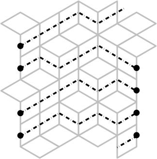
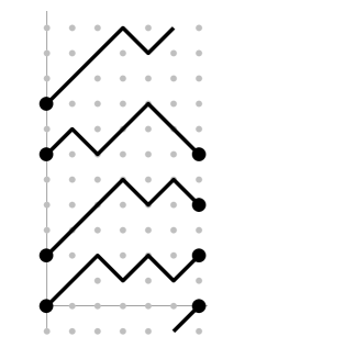
Figure 5: Conversion of the rhombic tiling (left) to a family of non-intersecting paths (right). Notice how the path starting from the left topmost starting point winds around the cylinder to connect to the bottom most ending point on the right.

These paths on the right of Figure 5, can be understood as the trajectories of a particle system evolving with time, flowing along the horizontal axis. Each vertical line $x=t$ represents the particle configuration. From time $t$ to time $t+1$, each of these particles jumps one unit down or up. Initially, the mutual distances between particles are even, and they will stay even at all times, but two particles will never be at the same site at the same time. Michael Fisher [Fisher(1984)] coined the term “vicious walkers” for this model of particles. More precisely, in his model, we start with a fixed number of particles, and at each time step, every particle moves one unit in the positive or the negative direction so that at no time two particles sit in the same place. Since we started with a cylindrical graph, these particles do not actually move along a line but actually along a circle with $2m$ sites. Due to the particular matching problem that we started with, namely, due to the fact that to the left and to the right of the cylinder there is a ring of pentagons, the starting points of the particles must come in pairs, with the particles in each pair at distance $2$, and the same applies to the end points.

Exact determinantal formulas have been given by Grabiner [Grabiner(2002)] to count various families of such paths and Krattenthaler [Krattenthaler(2004/07)] answered the question of computing the asymptotics for this number of paths, as the number of steps goes to infinity. To stick with the notation of [Krattenthaler(2004/07)], positions of particles on the circles will be labeled by half-integers. At $t=0$, and all the even times, the positions of all particles will be (distinct) integers between 0 and $m-1$, and at odd times, they will be odd multiples of $\frac{1}{2}$. If there are $k$ layers of hexagons, then the particle systems will evolve until time $k+1$.

Theorem 19 from [Krattenthaler(2004/07)] give the number of families of $n$ paths with a given starting and ending positions (or equivalently, the number of perfect matchings of $F(m,k)$, with a fixed configuration on the two $m$-gons at extremities). The starting and ending positions are recorded in two sequences of numbers $\eta=(\eta_{1},\dots,\eta_{n})$ and $\lambda=(\lambda_{1},\dots,\lambda_{n})$ respectively. We adapt it slightly to the context of $k+1$ time steps:

Theorem 4.1 ([Krattenthaler(2004/07)], Theorem 19).

Let $\eta=(\eta_{1},\dots,\eta_{n})$ be a vector of integers of half-integers with $m>\eta_{1}>\cdots>\eta_{n}\geq 0$ and $\lambda=(\lambda_{1},\dots,\lambda_{n})$ be a vector of integers of half-integers with $m>\lambda_{s+1}>\cdots>\lambda_{n}>\lambda_{1}>\cdots>\lambda_{s}\geq 0$ for some $s$. Then, as $k$ tends to $\infty$, in such a way that for all $j$, $k+1\equiv 2\eta_{j}+2\lambda_{j}\ [2]$, the number of perfect matchings of $F(m,k)$ with boundary configurations encoded by $\eta$ and $\lambda$ is asymptotically equal to

$$\frac{2^{n^{2}-n}}{nm^{n}}\left(2^{n}\prod_{j=1}^{n}\cos\frac{\pi(j-\frac{n+1}{2})}{m}\right)^{k+1}\prod_{1\leq h<t\leq n}\left(\sin\frac{\pi(\eta_{h}-\eta_{t})}{m}\cdot\left|\sin\frac{\pi(\lambda_{h}-\lambda_{t})}{m}\right|\right).$$ (4.1)

For getting the exact asymptotics for our problem, one would simply have to sum this formula over all possible starting and ending positions, that is, over all $\lambda$’s and $\eta$’s which have the property that their coordinates come in pairs, the two coordinates in each pair differing by $1$ (cyclically) and sum over $n$, as the number of paths is not fixed, but can be any even number up to $m$. Nevertheless, for fixed $m$, we are talking about a finite sum.

Clearly, not all choices of starting and ending points will contribute to the leading term of the asymptotics. Inspection of (4.1) shows that the relevant term in the formula is

$$\bigg{(}2^{n}\prod_{j=1}^{n}\cos\frac{\pi(j-\frac{n+1}{2})}{m}\bigg{)}^{k+1},$$

as everything else doesn’t depend on $k$. In order to find the leading order of the asymptotics, The task is thus to find the (even) $n$ which maximises

$$2^{n}\prod_{j=1}^{n}\cos\frac{\pi(j-\frac{n+1}{2})}{m}.$$ (4.2)

But after closer inspection, we notice (unsurprisingly!) that, by Remark 3.3, the quantity in Equation (4.2) is equal to $\lambda_{\text{max}}^{(p)}$ from (3.3) with $n+p=m$, and the value of $n$ maximizing (4.2) is $n_{0}=m-p_{0}=2\lfloor\frac{m+1}{3}\rfloor$.

We thus recovered from another method the value of the growth constant

$$\rho(m)=2^{2\lfloor\frac{m+1}{3}\rfloor}\prod_{j=1}^{2\lfloor\frac{m+1}{3}\rfloor}\cos\frac{\pi(j-\frac{n+1}{2})}{m}=\prod_{j=1}^{\lfloor(m+1)/3\rfloor}\left(2\cos\frac{\pi(2j-1)}{2m}\right)^{2},$$

as in Theorem 3.4.

5 The entropy of the family $(F(m,k))$

Recall that the graph $F(m,k)$ has $2m(k+2)$ vertices. The dimer entropy  [Friedland et al.(2008)Friedland, Krop, Lundow, and Markström, Friedland and Peled(2005)] $h(m)$ of the family $(F(m,k))_{k\geq 0}$ is defined as

$$h(m):=\limsup_{k\to\infty}\frac{\log\Phi(F(m,k))}{2m(k+2)}.$$

From the previous sections we deduce

$$h(m)=\frac{\log\rho(m)}{2m}.$$

Equivalently, it says that the number of matchings if $F(m,k)$ for $m$ fixed and $k\gg 1$ is of order $e^{kh(m)}$.

The quantity $h(m)$ can be written as a Riemann sum, which increases and converges to the corresponding integral as $m$ goes to infinity:

$$\mathbf{h}=\frac{-3}{2\pi}\int_{0}^{\pi/3}\log(2\sin t)\mathrm{d}t\simeq 0.1615329736\dots$$

which is the maximal entropy for ergodic Gibbs measure on uniform dimer configurations of the infinite hexagonal lattice [Kenyon(1997), Kenyon(2002)].

As $m=5$ or $6$, we see that the entropy for the family $F(m,k)$ is strictly smaller than $\mathbf{h}$. This is due to the geographic localisation of the pentagons in our family of fullerenes. However, if the pentagons are far enough from one another, their presence pentagons seems very unlikely to have a great nfluence on the number of perfect matchings of a large fullerene which would behave in this respect just as a the hexagonal lattice. That motivates us to advance the following conjecture:

Let $n$ be an integer number greater than $11$ so that there is a fullerene with $2n$ vertices. Denote by $\mu_{2n}$ the maximal number of perfect matchings in all fullerene graphs with $2n$ vertices. Define

$$h_{F}:=\limsup_{n\to\infty}\frac{\log\mu_{2n}}{2n}.$$

We conjecture that $h_{F}=\mathbf{h}$.

A similar claim seems plausible also for $m$-generalized fullerenes. Fix an integer $m\geq 3,m\neq 5,6$. Let $\mu_{2m(k+2),m}$ be the maximal number of perfect matchings in all $m$-generalized fullerene graphs with $2m(k+2)$ vertices. Define

$$h_{F}(m):=\limsup_{k\to\infty}\frac{\log\mu_{2m(k+2),m}}{2m(k+2)}.$$

We conjecture that $h_{F}(m)$ is also equal to $\mathbf{h}$ (and thus strictly greater than $h(m)$).

References

- [Andova et al.(2012)Andova, Došlić, Krnc, Lužar, and Škrekovski] V. Andova, T. Došlić, M. Krnc, B. Lužar, and R. Škrekovski. On the diameter and some related invariants of fullerene graphs. MATCH Commun. Math. Comput. Chem., 68(1):109–130, 2012. ISSN 0340-6253.
- [Behmaram and Friedland(2013)] A. Behmaram and S. Friedland. Upper bounds for perfect matchings in Pfaffian and planar graphs. Electron. J. Combin., 20(1):Paper 64, 16, 2013. ISSN 1077-8926.
- [Behmaram et al.(2016)Behmaram, Došlić, and Friedland] A. Behmaram, T. Došlić, and S. Friedland. Matchings in -generalized fullerene graphs. Ars Math. Contemp., 11(2):301–313, 2016. ISSN 1855-3966.
- [Bethe(1931)] H. Bethe. Zur theorie der metalle. Zeitschrift für Physik, 71(3):205–226, Mar 1931. ISSN 0044-3328. doi: 10.1007/BF01341708. URL https://doi.org/10.1007/BF01341708.
- [Došlić(2008)] T. Došlić. Leapfrog fullerenes have many perfect matchings. Journal of Mathematical Chemistry, 44(1):1–4, Jul 2008. ISSN 1572-8897. doi: 10.1007/s10910-007-9287-x. URL https://doi.org/10.1007/s10910-007-9287-x.
- [Došlić(2009)] T. Došlić. Finding more perfect matchings in leapfrog fullerenes. Journal of Mathematical Chemistry, 45(4):1130–1136, Apr 2009. ISSN 1572-8897. doi: 10.1007/s10910-008-9435-y. URL https://doi.org/10.1007/s10910-008-9435-y.
- [Fisher(1984)] M. E. Fisher. Walks, walls, wetting, and melting. J. Statist. Phys., 34(5-6):667–729, 1984. ISSN 0022-4715. doi: 10.1007/BF01009436. URL http://dx.doi.org/10.1007/BF01009436.
- [Friedland and Peled(2005)] S. Friedland and U. N. Peled. Theory of computation of multidimensional entropy with an application to the monomer–dimer problem. Advances in Applied Mathematics, 34(3):486–522, apr 2005. doi: 10.1016/j.aam.2004.08.005. URL https://doi.org/10.1016/j.aam.2004.08.005.
- [Friedland et al.(2008)Friedland, Krop, Lundow, and Markström] S. Friedland, E. Krop, P. H. Lundow, and K. Markström. On the validations of the asymptotic matching conjectures. Journal of Statistical Physics, 133(3):513–533, Nov 2008. ISSN 1572-9613. doi: 10.1007/s10955-008-9550-y. URL https://doi.org/10.1007/s10955-008-9550-y.
- [Gessel and Viennot(1985)] I. Gessel and G. Viennot. Binomial determinants, paths, and hook length formulae. Adv. in Math., 58(3):300–321, 1985. ISSN 0001-8708.
- [Grabiner(2002)] D. J. Grabiner. Random walk in an alcove of an affine Weyl group, and non-colliding random walks on an interval. J. Combin. Theory Ser. A, 97(2):285–306, 2002. ISSN 0097-3165. doi: 10.1006/jcta.2001.3216. URL http://dx.doi.org/10.1006/jcta.2001.3216.
- [Grünbaum and Motzkin(1963)] B. Grünbaum and T. S. Motzkin. The number of hexagons and the simplicity of geodesics on certain polyhedra. Canad. J. Math., 15:744–751, 1963. ISSN 0008-414X. doi: 10.4153/CJM-1963-071-3. URL http://dx.doi.org/10.4153/CJM-1963-071-3.
- [Kardoš et al.(2009)Kardoš, Král’, Miškuf, and Sereni] F. Kardoš, D. Král’, J. Miškuf, and J.-S. Sereni. Fullerene graphs have exponentially many perfect matchings. Journal of Mathematical Chemistry, 46(2):443–447, Aug 2009. ISSN 1572-8897. doi: 10.1007/s10910-008-9471-7. URL https://doi.org/10.1007/s10910-008-9471-7.
- [Karlin and McGregor(1959)] S. Karlin and J. McGregor. Coincidence probabilities. Pacific J. Math., 9:1141–1164, 1959. ISSN 0030-8730.
- [Kenyon(1997)] R. Kenyon. Local statistics of lattice dimers. Ann. Inst. H. Poincaré Probab. Statist., 33(5):591–618, 1997. ISSN 0246-0203.
- [Kenyon(2002)] R. Kenyon. The Laplacian and Dirac operators on critical planar graphs. Invent. Math., 150(2):409–439, 2002. ISSN 0020-9910.
- [Krattenthaler(2004/07)] C. Krattenthaler. Asymptotics for random walks in alcoves of affine Weyl groups. Sém. Lothar. Combin., 52:Art. B52i, 72, 2004/07. ISSN 1286-4889.
- [Kroto et al.(1985)Kroto, Heath, Obrien, Curl, and Smalley] H. W. Kroto, J. R. Heath, S. C. Obrien, R. F. Curl, and R. E. Smalley. C(60): Buckminsterfullerene. Nature, 318:162, Nov. 1985. doi: 10.1038/318162a0.
- [Kutnar and Marušič(2008)] K. Kutnar and D. Marušič. On cyclic edge-connectivity of fullerenes. Discrete Appl. Math., 156(10):1661–1669, 2008. ISSN 0166-218X. doi: 10.1016/j.dam.2007.08.046. URL http://dx.doi.org/10.1016/j.dam.2007.08.046.