On complexity of multidistance graph recognition in $\mathbb{R}^{1}$

Abstract

Let $\mathcal{A}$ be a set of positive numbers. A graph $G$ is called an $\mathcal{A}$-embeddable graph in $\mathbb{R}^{d}$ if the vertices of $G$ can be positioned in $\mathbb{R}^{d}$ so that the distance between endpoints of any edge is an element of $\mathcal{A}$. We consider the computational problem of recognizing $\mathcal{A}$-embeddable graphs in $\mathbb{R}^{1}$ and classify all finite sets $\mathcal{A}$ by complexity of this problem in several natural variations.

1 Introduction

1.1 Problem statement and motivation

Let $\mathcal{A}\subseteq\mathbb{R}_{>0}$ be a set of admissible distances. For a set of points $S\subseteq\mathbb{R}^{d}$ we construct an $\mathcal{A}$-distance graph of $S$ as a graph with vertices in $S$ and edges between all pairs of vertices at admissible distances. A generic graph will be called an $\mathcal{A}$-distance graph in $\mathbb{R}^{d}$ if it is isomorphic to an $\mathcal{A}$-distance graph of a subset of $\mathbb{R}^{d}$.

The notion of an $\mathcal{A}$-distance graph is inspired by classic unit-distance graphs and is, indeed, a proper generalization since putting $\mathcal{A}=\{1\}$ yields exactly the unit-distance graphs. Unit-distance graphs appear in many classical problems such as Erdős’ unit distance problem (see [1]), Nelson—Hadwiger problem of the chromatic number of the plane (see [2]). For a comprehensive survey of these (and many other) discrete geometry problems see [3]; a survey of results concerning unit-distance graphs can be found in [4, 5, 6]. Some isolated properties of $\mathcal{A}$-distance graphs were studied for finite sets $\mathcal{A}$ (see [4, 7, 8]).

In literature unit-distance graphs and objects of similar nature appear under different names, such as linkages ([9]), embeddable ([10]), or realizable ([9]) graphs. Also, the term “unit-distance graph” is sometimes applied to slightly different objects (e.g., in [11]). Before going further, we find it convenient to unify the different notions and extend them to the multidistance case.

Let $G=(V(G),E(G))$ be a graph. If $\varphi:V(G)\to\mathbb{R}^{d}$ is such a map that Euclidean distance between $\varphi(x)$ and $\varphi(y)$ is an element of $\mathcal{A}$ for all edges $xy\in E(G)$, then we will say that $\varphi$ is an $\mathcal{A}$-embedding of $G$ in $\mathbb{R}^{d}$. We will call $\varphi$ an injective $\mathcal{A}$-embedding if it maps distinct vertices to distinct points of $\mathbb{R}^{d}$ (that is, $\varphi$ is an injective map). If for any pair $xy\not\in E(G)$ we have that the distance between $\varphi(x)$ and $\varphi(y)$ is not an element of $\mathcal{A}$, then $\varphi$ will be called a strict $\mathcal{A}$-embedding. Naturally, a graph is (strictly) (injectively) $\mathcal{A}$-embeddable in $\mathbb{R}^{d}$ if it admits an (strict) (injective) $\mathcal{A}$-embedding in $\mathbb{R}^{d}$. Note that strictly injectively $\mathcal{A}$-embeddable graphs are exactly the $\mathcal{A}$-distance graphs as defined above.

We now consider the computational problem of recognizing $\mathcal{A}$-embeddable graphs in $\mathbb{R}^{d}$. Throughout the paper we consider the distance set $\mathcal{A}$, the dimension $d$, as well as the choice of one of the embeddability types (arbitrary, strict, injective, strict and injective) to be fixed parameters and not parts of the input.

The complexity of the unit-distance ($\mathcal{A}=\{1\}$) case is studied in [10, 11, 9, 12]: all variations of the problem are in P for $d=1$, and are NP-hard for $d\geqslant 2$. Another example of a well-studied case is the case of $(0,1]$-distance graphs, usually called unit ball graphs. In the $d=1$ case (real line embedding) $(0,1]$-distance graphs are unit interval graphs; they are recognizable in linear time ([13, 14]). Recognizing $(0,1]$-distance graphs in the plane is NP-hard ([15]) and even hard for the existential theory of reals ([16]). An interesting approach of [17] based on dense lattices in $\mathbb{R}^{d}$ allows to establish NP-hardness of $(0,1]$-embeddability for $d=3,4,8,24$.

The present paper is concerned with the most “primitive” case of the $\mathcal{A}$-embeddable graph recognition problem with $d=1$ and finite distance sets. For each finite set $\mathcal{A}$ and each embedding type we classify the corresponding problem as belonging to P or an NP-complete. Note that since the set $\mathcal{A}$ is fixed, all functions that depend only on $\mathcal{A}$ rather than on the input graph are constant in complexity estimates.

1.2 Statement of the results

Let $\mathcal{A}$ be a non-empty finite set of non-zero real numbers. Suppose further that $\mathcal{A}=-\mathcal{A}$, that is, $x\in\mathcal{A}$ implies $-x\in\mathcal{A}$. Let $G=\langle\mathcal{A}\rangle_{+}$ be the additive group generated by elements of $\mathcal{A}$. A graph $X$ is $\mathcal{A}$-embeddable in $\mathbb{R}^{1}$ if and only if a homomorphism of certain type exists between the graphs $X$ and $\Gamma=\mathrm{Cay}(G,\mathcal{A})$ — the Cayley graph of the group $G$ with the generating set $\mathcal{A}$. We recall that by definition $\Gamma=(V(\Gamma),E(\Gamma))$ with $V(\Gamma)=G$ and $E(\Gamma)=\{\{x,gx\}\mid x\in G,g\in\mathcal{A}\}$.

The group $G$ is a free finitely generated abelian group, hence it is isomorphic to $\mathbb{Z}^{k}$ for an integer $k\geqslant 1$. In the sequel we identify each element of $G$ with the element of $\mathbb{Z}^{k}$ being its image under a certain canonically chosen group isomorphism.

The following theorem provides a complete classification of finite sets $\mathcal{A}$ depending on the complexity of $\mathcal{A}$-embeddability checking in $\mathbb{R}^{1}$.

Theorem 1.

1. The problem of $\mathcal{A}$-embeddability checking in $\mathbb{R}^{1}$ is in P if the graph $\Gamma$ is bipartite, otherwise the problem is NP-complete.

2. The problem of strict and/or injective $\mathcal{A}$-embeddability checking in $\mathbb{R}^{1}$ is in P if $\langle\mathcal{A}\rangle_{+}\sim\mathbb{Z}$, otherwise the problem is NP-complete.

Note that $\langle\mathcal{A}\rangle_{+}\sim\mathbb{Z}$ if and only if all pairwise quotients of elements of $\mathcal{A}$ are rational, or, equivalently, $\mathcal{A}\subset\alpha\mathbb{Z}$ for a real $\alpha\neq 0$.

The (a) part of Theorem 1 is an immediate corollary of the result [18] on the complexity of $H$-coloring for infinite graphs $H$ of bounded degree. It is possible to obtain a more explicit condition in terms of elements of $\mathcal{A}$:

Proposition 1.2.1.

If $\mathcal{A}\subset\mathbb{Z}^{k}$ is a symmetrical generating set of $\mathbb{Z}^{k}$, then $\Gamma=\mathrm{Cay}(\mathbb{Z}^{k},\mathcal{A})$ is bipartite iff there is a subset $I\subseteq\{1,\ldots,k\}$ such that for each $x=(x_{1},\ldots,x_{k})\in\mathcal{A}$ we have that $\sum_{i\in I}x_{i}$ is odd.

Proof.

If there is a set $I$ that satisfies the premise, then $\Gamma$ is bipartite with parts $\{G_{0},G_{1}\}$ defined by $G_{j}=\{x\in\mathbb{Z}^{k}|\sum_{i\in I}x_{i}\equiv j\leavevmode\nobreak\ (\bmod\leavevmode\nobreak\ 2)\}$. Conversely, let $\Gamma$ be bipartite with parts $\{G_{0},G_{1}\}$, i.e. $G_{0},G_{1}\subseteq\mathbb{Z}^{k}$, $G_{0}\cup G_{1}=\mathbb{Z}^{k}$, $G_{0}\cap G_{1}=\varnothing$, and for any edge $xy$ of $\Gamma$ neither $G_{0}$ nor $G_{1}$ contains both $x$ and $y$. Note that if $\Gamma$ is bipartite, then there is only one correct partition. Without loss of generality, assume that $0\in G_{0}$. Consider a basis element $e_{i}\in\mathbb{Z}^{k}$, with all coordinates except $i$-th equal to 0, and $i$-th coordinate equal to 1. If $e_{i}\in G_{0}$, then by vertex transitivity we must have that for any $x\in\mathbb{Z}^{k}$ the elements $x$ and $x+e_{i}$ belong to the same part. If $e_{i}\in B$, then $x$ and $x+e_{i}$ must belong to different parts for any $x$. Define $I=\{i\in\{1,\ldots,k\}|e_{i}\in G_{1}\}$. For any element $x\in\mathcal{A}$ we must have $x\in G_{1}$ since $0x$ is an edge of $\Gamma$, hence $\sum_{i\in I}x_{i}$ is odd, which concludes the proof.

∎

The case $\langle\mathcal{A}\rangle_{+}\sim\mathbb{Z}$ of the (b) part follows from the result [19] on the time-polynomial solution of SUBGRAPH-ISOMORPHISM for graphs of bounded treewidth; the details are given in Section 1.3 (a discussion of treewidth and a survey of relevant algorithmic results can be found in [20]). The bulk of the present paper is dedicated to proving NP-completeness of strict and/or injective $\mathcal{A}$-embeddability checking in $\mathbb{R}^{1}$ in the case $\langle\mathcal{A}\rangle_{+}\sim\mathbb{Z}^{k}$ with $k\geqslant 2$. Let us outline the scheme of the proof.

In Section 2 we study automorphisms of the Cayley graph $\Gamma$ and its finite subgraphs. The main result of the section is Theorem 2 that asserts existence of finite subgraphs of $\Gamma$ such that each of their automorphisms acts linearly on elements of $\mathbb{Z}^{k}$ and can be extended uniquely to an automorphism of the full graph $\Gamma$. The existence of “$\Gamma$-rigid” subgraphs provided by Theorem 2 allows us to avoid most of the complications arising from the “graphical” nature of $\mathcal{A}$-embeddability and lead the discussion of the subsequent constructions in geometric terms.

In order to establish NP-completeness, we implement the “logic engine” setup (see Section 3.1) to reduce from the NP-complete NAE-3-SAT problem to strict and/or injective $\mathcal{A}$-embeddability checking via an intermediate problem LOGIC-ENGINE. In Section 3 we describe the reduction from logic engine realizability to each case of strict and/or injective $\mathcal{A}$-embeddability checking in $\mathbb{R}^{1}$ using two different logic engine implementations for the cases $k=2$ and $k>2$.

Note that all embeddability problems in $\mathbb{R}^{1}$ belong to NP since they are equivalent to the $\Gamma$-coloring problem (with possible additional constraints) which admits polynomial certificate, namely, integer coordinates of corresponding elements of $\mathbb{Z}^{k}$.

1.3 The $G\sim\mathbb{Z}$ case, strict and/or injective $\mathcal{A}$-embeddability

Since $\langle\mathcal{A}\rangle=\mathbb{Z}$, the elements of $\mathcal{A}$ become mutually coprime integers under a canonical group isomorphism of $G$ and $\mathbb{Z}$. Let us put $D=\max\{|x|:x\in\mathcal{A}\}$.

First consider the injective (possibly non-strict) embeddability case.

Lemma 1.3.1.

Let $H$ be a finite subgraph of $\Gamma=\mathrm{Cay}(\mathbb{Z},\mathcal{A})$. Then the treewidth (and, moreover, the pathwidth) of $H$ is at most $D$.

Proof.

Note that adding edges to a graph does not decrease its path- or treewidth. Without loss of generality, suppose that the subgraph $H=(V,E)$ is induced by a vertex set $V=\{0,\ldots,M\}$. If $M<D$, then take the trivial path decomposition with a single vertex $V$. This decomposition has width $M<D$, hence the claim holds.

Now suppose that $M\geqslant D$. We will build a path decomposition $P$ of the graph $H$ with width $D$. Take subsets $A_{x}=\{x,\ldots,x+D\}$ for all integer $x$ from 0 to $M-D$ as vertices of $P$. The edges of $P$ will connect subsets that are different in a single element.

Let us ensure that $P$ is indeed a path decomposition of $H$. Clearly $P$ is a path, and for every vertex $x\in V$ the vertices of $P$ containing $x$ form a subpath. Suppose that $xy\in E$ and $x<y$. Then $y\leqslant x+D$ and $x,y\in A_{x}$, hence both endpoints of any edge of $H$ are covered by a vertex of $P$. Thus all requirements of a path decomposition are met. Finally, it can easily be seen that the width of $P$ is $D$.

∎

Suppose that a connected graph $X=(V(X),E(X))$ is the input to the $\mathcal{A}$-embeddability checking problem, and $Y$ is a subgraph of $\Gamma$ induced by the vertex set {$0$, …, $|V(X)|\cdot D$}. Clearly, the graph $X$ is (strictly/non-strictly) injectively $\mathcal{A}$-embeddable in $\mathbb{R}^{1}$ if and only if $X$ is isomorphic to an (induced/non-induced) subgraph of $Y$.

The following result is due to [19]: suppose that the maximal degree of a connected graph $X$ is bounded by a constant $\Delta$, and a graph $Y$ has treewidth bounded by a constant $k$, then finding an (induced/non-induced) subgraph of $Y$ that is isomorphic to $X$ can be done in $O(|V(X)|^{k+1}|V(Y)|)$ time. The maximal degree of the graph $Y$ is at most $2D$, thus we can assume that the maximal degree of $X$ is at most $2D$ as well (otherwise $X$ can not be isomorphic to a subgraph of $Y$). Further, by the previous lemma the treewidth of $Y$ is at most $D$. Thus, by using the algorithm of [19], we obtain an algorithm for checking injective (strict/non-strict) $\mathcal{A}$-embeddability in $O(|V(X)|^{D+2})$ time.

Finally, consider the case of strict non-injective $\mathcal{A}$-embeddability. Let $N(v)$ denote the set of neighbours of a vertex $v$ in the graph $X$. We will say that vertices $v,u\in V(X)$ are equivalent if $N(v)=N(u)$, and will write $v\sim u$.

Proposition 1.3.2.

Suppose that $V^{\prime}$ is a subset of $V(X)$ that contains a single vertex from each equivalence class of $V(X)$, and $X^{\prime}$ is the subgraph of $X$ induced by $V^{\prime}$. Then the graph $X$ is strictly $\mathcal{A}$-embeddable in $\mathbb{R}^{1}$ if and only if $X^{\prime}$ is strictly injectively $\mathcal{A}$-embeddable in $\mathbb{R}^{1}$.

Proof.

Suppose that $\varphi$ is a strict $\mathcal{A}$-embedding of $X$ in $\mathbb{R}^{1}$. If $\varphi(v)=\varphi(u)$, then by strictness of $\varphi$ for every other vertex $w\in V(X)$ the edges $vw$ and $uw$ are either both inside or both outside of $E(X)$, and we must have $v\sim u$. Since no two distinct vertices of $V^{\prime}$ are equivalent, then the restriction $\varphi|_{V^{\prime}}$ is a suitable strict injective $\mathcal{A}$-embedding of the graph $X^{\prime}$.

Conversely, consider a strict injective $\mathcal{A}$-embedding $\varphi^{\prime}$ of the graph $X^{\prime}$ in $\mathbb{R}^{1}$. Define an embedding $\varphi:V(X)\to V(\Gamma)$ by $\varphi(v)=\varphi^{\prime}(R(v))$, where $R(v)$ is the only vertex of $V^{\prime}$ that satisfies $v\sim R(v)$. If $vu\in E(X)$, then we must have $R(v)R(u)\in E(X)$. But $\varphi$ is strict, hence $\varphi(x)-\varphi(y)=\varphi(R(x))-\varphi(R(y))\in\mathcal{A}$, thus $\varphi$ is a strict $\mathcal{A}$-embedding.

∎

The graph $X^{\prime}$ can be easily constructed by $X$ in polynomial time, and strict injective $\mathcal{A}$-embeddability of $X^{\prime}$ can be checked in polynomial time in the $k=1$ case. Thus the first half of the (b) part of Theorem 1 is proven.

2 Balls in $\Gamma$ and their automorphisms

2.1 Balls and embeddings

Recall that $G\sim\mathbb{Z}^{k}$ is a free finitely generated abelian group, $\mathcal{A}$ is a finite generating set of $G$, and $\Gamma=\mathrm{Cay}(G,\mathcal{A})$.

Let $x,y\in G$. Since for each $d\in G$ the translation $x\rightarrow x+d$ is an automorphism of $\Gamma$, the length of the shortest path between vertices $x$ and $y$ in the graph $\Gamma$ depends only on $x-y$; let $\rho^{\mathcal{A}}(x-y)$ denote this length ($\rho^{\mathcal{A}}$ is the same as the word metric of the group $G$ with the generating set $\mathcal{A}$). Also let $\omega^{\mathcal{A}}(x-y)$ denote the number of shortest paths between $x$ and $y$ in $\Gamma$. In the sequel we will omit the upper index $\mathcal{A}$ when the set $\mathcal{A}$ is clear from the context.

If $x\in G$ and $V\subset G$, then we will write $V+x$ for a copy of $V$ translated by $x$ element-wise. Similarly, if $\lambda$ is a subgraph of $\Gamma$, we will write $\lambda+x$ for a subgraph obtained from $\lambda$ by shifting all vertices and endpoints of edges by $x$.

Definition 2.1.1.

Suppose that $r$ is a non-negative integer. Let $B^{\mathcal{A}}_{r}$ denote the subgraph of $\Gamma$ induced by the vertex set $V(B^{\mathcal{A}}_{r})=\{x\in G:\rho^{\mathcal{A}}(x)\leqslant r\}$. We will call the graph $B^{\mathcal{A}}_{r}$ the ball of radius $r$.

Proposition 2.1.2.

Suppose that $\lambda$ is a subgraph of $\Gamma$, and $\varphi:B_{r}\to\lambda$ is a graph isomorphism. Then $\lambda=B_{r}+\varphi(0)$.

Proof.

Since for any path $v_{0}$, …, $v_{s}$ in the graph $B_{r}$ there is a path $\varphi(v_{0})$, …, $\varphi(v_{s})$ in the graph $\lambda$, then for any vertex $x\in V(B_{r})$ we have

$$\rho(\varphi(x)-\varphi(0))\leqslant\rho(x)\leqslant r,$$

hence $V(\lambda)\subseteq V(B_{r}+\varphi(0))$. But

$$|V(\lambda)|=|V(B_{r})|=|V(B_{r}+\varphi(0))|,$$

thus we have $V(\lambda)=V(B_{r}+\varphi(0))$. Edges of $B_{r}$ and $\lambda$ are in one-to-one correspondence, thus

$$|E(B_{r})|=|E(\lambda)|\leqslant|E(B_{r}+\varphi(0))|=|E(B_{r})|,$$

and $E(\lambda)=E(B_{r}+\varphi(0))$.

∎

We are interested in possible embeddings of the ball of radius $r$ in the graph $\Gamma$, that is, graph isomorphisms $\varphi:B_{r}\to B_{r}+\varphi(0)$. Since $\Gamma$ is vertex-transitive, it suffices to consider the group $\mathrm{Aut}(B_{r})$, because every embedding $\varphi$ is composed of an automorphism of $B_{r}$ and a translation by $\varphi(0)$.

Consider the group $\mathrm{Aut}_{0}(\Gamma)$ of automorphisms of $\Gamma$ that stabilize the origin. It follows from the results of [21] that each automorphism $\varphi\in\mathrm{Aut}_{0}(\Gamma)$ is additive (that is, satisfies $\varphi(x+y)=\varphi(x)+\varphi(y)$ for all $x,y\in G$), hence it is unambigiosly determined by the values $\varphi(a)$ on all $a\in\mathcal{A}$.

Linearity is a stronger property of an automorphism. We will say that $\varphi\in\mathrm{Aut}_{0}(\Gamma)$ is linear if there exists a non-degenerate linear map $T:\mathbb{R}^{k}\to\mathbb{R}^{k}$ such that $\varphi(x)=T(x)$ for all $x\in G$. Clearly, linearity implies additivity.

From each $\varphi\in\mathrm{Aut}_{0}(\Gamma)$ we can construct an element of $\mathrm{Aut}(B_{r})$, namely, the restriction $\varphi|_{V(B_{r})}$. Since an element of $\mathrm{Aut}_{0}(\Gamma)$ is induced by its values on $\mathcal{A}$, we have that distinct elements of $\mathrm{Aut}_{0}(\Gamma)$ have distinct restrictions on $B_{r}$ (if $r$ is positive). It should be noted, however, that in many cases the graph $B_{r}$ admits different kinds of automorphisms: for example, if $\mathcal{A}$ is a standard basis of $\mathbb{Z}^{k}$ (after adjoining the inverse elements) and $r=1$, then the group $\mathrm{Aut}_{0}(\Gamma)$ is isomorphic to $S_{k}\times\mathbb{Z}_{2}^{k}$ since each automorphism can freely exchange the axes and/or flip their directions. At the same time, we have that $\mathrm{Aut}(B_{r})$ is isomorphic to $S_{2k}$ since the graph $B_{r}$ is isomorphic to $K_{1,2k}$. Moreover, for each integer $r>0$ we can construct a set $\mathcal{A}$ such that $\mathrm{Aut}(B_{r})\not\sim\mathrm{Aut}_{0}(\Gamma)$: if we take, for example,

$$\mathcal{A}=\{\pm(2r+1,0),\pm(0,2r+2),\pm(1,1)\},$$

then the graph $B_{r}$ is isomorphic to a ball of radius $r$ in the lattice $\mathbb{Z}^{3}$ with standard basis, hence $\mathrm{Aut}(B_{r})\sim S_{3}\times\mathbb{Z}_{2}^{3}$, while $\mathrm{Aut}_{0}(\Gamma)\sim\mathbb{Z}_{2}$ and contains only the trivial automorphism and the central symmetry.

Theorem 2 shows that for sufficiently large radius $r$ the group $\mathrm{Aut}(B_{r})$ precisely captures the structure of $\mathrm{Aut}_{0}(\Gamma)$, or, in other words, each automorphism of $B_{r}$ can be extended to an automorphism of $\Gamma$ (in this case, the extension is unique). Moreover, all automorphisms of $B_{r}$ and $\Gamma$ turn out to be linear.

Theorem 2.

Suppose that $G$ is a free finitely generated abelian group, and $\mathcal{A}\subset G$ is an arbitrary finite symmetrical generating set of $G$ that doesn’t contain 0. Then there exists an integer $R(\mathcal{A})$ such that for every integer $r\geqslant R(\mathcal{A})$ each automorphism of the graph $B_{r}$ is linear and has a unique extension to an element of $\mathrm{Aut}_{0}(\mathrm{Cay}(G,\mathcal{A}))$.

Let us outline the proof of Theorem 2. First, we establish that each automorphism of a sufficiently large ball stabilizes the set of vertices of convex hull of $\mathcal{A}$ (these vertices are called the primary elements of $\mathcal{A}$). We will refer to the corresponding permutation of primary elements of $\mathcal{A}$ as an orientation of the automorphism. We also show that orientation is well-defined for any “bundle” of balls, that is, the induced union of balls with a connected set of centers. We will use this to show that each automorphism of a large enough ball is linear on the partial lattice induced by primary elements.

On the other hand, we will show that the restriction of any automorphism to the lattice induced by non-primary (secondary) elements is an automorphism of the ball in the Cayley graph of the additive group induced by the secondary elements. By induction on the size of $\mathcal{A}$, this implies linearity of this automorphism if the ball is large enough. The final part of the proof is “gluing” of the two linear automorphisms and extending them to all vertices of the ball that do not belong to any of the lattices. Finally, we exclude each automorphism of $B_{r}$ that does not allow extension to an automorphism of $\Gamma$ simply by increasing $r$ since the set of permutations of $\mathcal{A}$, and therefore, of possible automorphisms, is finite.

2.2 Properties of ball embeddings in $\Gamma$

Proposition 2.2.1.

For each graph automorphism $\varphi:B_{r}\to B_{r}+\varphi(0)$ and each vertex $x\in V(B_{r})$ the equalities $\rho(\varphi(x)-\varphi(0))=\rho(x)$ and $\omega(\varphi(x)-\varphi(0))=\omega(x)$ hold.

Proof.

For each ball subgraph $B_{r}+z$ any shortest path in $\Gamma$ between the center $z$ and any vertex of $B_{r}+z$ contains only edges of $B_{r}+z$, hence there is a bijection between shortest paths in $\Gamma$ from $0$ to $x$ and from $\varphi(0)$ to $\varphi(x)$.

∎

Definition 2.2.2.

We will say that $x\in\mathcal{A}$ is a primary element if for any integer $t\geqslant 0$ we have $\rho(tx)=t$ and $\omega(tx)=1$. Any other element of $\mathcal{A}$ will be a secondary element.

Let $\mathcal{A}^{\prime}$ denote the set of all primary elements of $\mathcal{A}$. It is clear from the symmetry argument that $\mathcal{A}^{\prime}=-\mathcal{A}^{\prime}$.

By definition, there exists an integer $D$ such that for all secondary $x\in\mathcal{A}$ we have either $\rho(Dx)\neq D$ or $\omega(Dx)\neq 1$. Aside from characterization of primary elements of $\mathcal{A}$, the next proposition contains a constructive way of choosing a suitable value of $D$ in the second part of the proof.

If $V\subset\mathbb{R}^{n}$, then we will write $\mathrm{Conv}\,V$ for the convex hull of the set $V$.

Proposition 2.2.3.

An element $x\in\mathcal{A}$ is primary if and only if $x$ is a vertex of $\mathrm{Conv}\,\mathcal{A}$.

Proof.

Let $x$ be a vertex of $\mathrm{Conv}\,\mathcal{A}$, then there is a linear function $l:\mathbb{R}^{k}\to\mathbb{R}$ such that $l(x)>l(y)$ for all $y\in\mathcal{A}$ that are different from $x$. It follows that $l(x)>l(-x)=-l(x)$, and $l(x)>0$. Suppose that $d_{1},\ldots,d_{s}\in\mathcal{A}$ is a sequence of edge transitions in $\Gamma$ leading from 0 to $tx$, that is, $d_{1}+\ldots+d_{s}=tx$. Then we have

$$tl(x)=l(tx)=l(d_{1})+\ldots+l(d_{s})\leqslant sl(x),$$

hence $s\geqslant t$ and $\rho(tx)\geqslant t$. If $s=t$ and not all elements $d_{1}$, …, $d_{t}$ are equal to $x$, then $l(d_{1})+\ldots+l(d_{t})<tl(x)$, a contradiction. Thus the shortest path in $\Gamma$ between 0 to $tx$ has length $t$ and is unique, hence $x$ is indeed a primary element.

Now suppose that $x$ is not a vertex of $\mathrm{Conv}\,\mathcal{A}$. Note that the origin of $\mathbb{R}^{k}$ lies inside of $\mathrm{Conv}\,\mathcal{A}$ since $\mathcal{A}=-\mathcal{A}$. Then $x$ belongs to the convex hull of the origin and a certain set $y_{1},\ldots,y_{s}\in\mathcal{A}$ (with all ${y_{i}\neq x}$) over the field $\mathbb{Q}$. Hence we have $x=\sum\alpha_{i}y_{i}$ for some non-negative rational numbers $\alpha_{i}$ such that $\sum\alpha_{i}\leqslant 1$. After multiplying by a common denominator of the numbers $\alpha_{i}$ we obtain the equality $Kx=\sum A_{i}y_{i}$, where $K$ and all $A_{i}$ are non-negative integers, and $0<\sum A_{i}\leqslant K$. From this equality we obtain that there is a path in $\Gamma$ between 0 and $Kx$ of length at most $K$ that contains transitions other than $x$, thus $\varphi(Kx)<K$ or $\omega(Kx)\neq 1$, and $x$ is not a primary element.

∎

From the second part of the proof we can also obtain the following

Proposition 2.2.4.

For each element $x\in\mathcal{A}$ there exists an integer $K_{x}$ such that $K_{x}x$ can be represented as a sum of at most $K_{x}$ primary elements (with repetitions allowed).

The next proposition can be informally stated as follows: in any embedding of a large enough ball in $\Gamma$ the “rays” (i. e., the unique shortest paths) that correspond to the primary directions are <<rigid>> and can only be permuted among themselves, while opposite rays stay opposite and form a “straight line”.

Proposition 2.2.5.

Suppose that $r\geqslant\max(2,D)$ and $\varphi:B_{r}\to B_{r}+\varphi(0)$ is a graph isomorphism. Then for each $x\in\mathcal{A}^{\prime}$ there exists $x^{\prime}\in\mathcal{A}^{\prime}$ such that $\varphi(rx)-\varphi(0)=rx^{\prime}$. Moreover, $\varphi(tx)-\varphi(0)=tx^{\prime}$ for all integer $t\in[-r,r]$.

Proof.

Proposition 2.2.1 implies that

$$\rho(\varphi(rx)-\varphi(0))=\rho(rx)=r$$

and

$$\omega(\varphi(rx)-\varphi(0))=\omega(rx)=1.$$

However, if $\varphi(rx)-\varphi(0)\neq rx^{\prime}$ for all $x^{\prime}\in\mathcal{A}$, then we must have $\omega(\varphi(rx)-\varphi(0))\neq 1$. Indeed, an arbitrarily chosen shortest path from $\varphi(0)$ to $\varphi(rx)$ must contain different transitions, thus by permuting them we obtain a different shortest path. Therefore we have $\varphi(rx)-\varphi(0)=rx^{\prime}$ for a certain $x^{\prime}\in\mathcal{A}$. Moreover, $r\geqslant D$, thus $x^{\prime}$ is a primary element by the choice of $D$.

Next, let us establish the second part of the statement for $t=-r$, that is,

$$\varphi(-rx)-\varphi(0)=-rx^{\prime}.$$

Suppose that $\varphi(-rx)-\varphi(0)=rx^{\prime\prime}$ with $x^{\prime\prime}\neq-x^{\prime}$. Note that there is a unique path of length $2r$ between $rx$ and $-rx$ in the graph $B_{r}$ since $x$ is a primary element. At the same time, consider the following path of length $2r$ from $\varphi(rx)=\varphi(0)+rx^{\prime}$ to $\varphi(-rx)=\varphi(0)+rx^{\prime\prime}$ that passes through $\varphi(0)$: $r$ transitions by $-x^{\prime}$ followed by $r$ transitions by $x^{\prime\prime}$. Let us exchange $r$-th and $(r+1)$-th step of this path, the resulting path will pass through $\varphi(0)+x^{\prime\prime}-x^{\prime}$ instead of $\varphi(0)$. Since $r\geqslant 2$ and $\rho(x^{\prime\prime}-x^{\prime})\leqslant 2$, the new path lies completely inside of $B_{r}+\varphi(0)$, and thus we have at least two different paths of length $2r$ between $\varphi(rx)$ and $\varphi(-rx)$ in $B_{r}+\varphi(0)$. It follows that the graph isomorphism $\varphi$ does not preserve the number of paths of length $2r$ between a pair of vertices, which is a contradiction. Hence we have $\varphi(-rx)-\varphi(0)=-rx^{\prime}$.

Finally, let us prove the second part for all other values of $t$. First, let $t\geqslant 0$. The vertex $\varphi(tx)$ must belong to the only shortest path between $\varphi(0)$ and $\varphi(rx)$. But this path consists only of transitions by $x^{\prime}$, hence $\varphi(tx)-\varphi(0)=tx^{\prime}$. The $t\leqslant 0$ case is handled similarly by considering the shortest path between $\varphi(0)$ and $\varphi(-rx)$.

∎

Let us define the orientation of a ball embedding as a way of permuting the primary elements.

Definition 2.2.6.

Suppose that $r\geqslant\max(2,D)$ and $\varphi:B_{r}+z\to B_{r}+\varphi(z)$ is a graph isomorphism. Let $\chi^{\varphi}$ denote the orientation of the isomorphism $\varphi$ as a function that maps each $x\in\mathcal{A}^{\prime}$ to $\varphi(x+z)-\varphi(z)$. If $\varphi:X\to Y$ is an isomorphism between two subgraphs of $\Gamma$, and $B_{r}+z$ is a subgraph of $X$, let us write $\chi^{\varphi}_{B_{r}+z}$ for the orientation of the restriction of $\varphi$ to $B_{r}+z$.

Proposition 2.2.5 immediately implies

Corollary 2.2.7.

$\chi^{\varphi}$ is a permutation of $\mathcal{A}^{\prime}$ that satisfies $\chi^{\varphi}(x)=-\chi^{\varphi}(-x)$.

Definition 2.2.8.

For $x\in G$ define the norm $||x||$ as an $l_{\infty}$-norm of the corresponding element of $\mathbb{Z}^{k}$ (i. e., the largest absolute value of coordinates). For a subset $V\subset G$ put $||V||=\max_{x\in V}||x||$.

The next proposition states that if two large enough balls (possibly having common vertices) are subgraphs of an induced subgraph of $\Gamma$, and the centers of the balls are adjacent, then their orientations must coincide in any embedding of the subgraph.

Proposition 2.2.9.

Suppose that $r\geqslant\max(2,D,2||\mathcal{A}||+1)$. Suppose further that ${z\in\mathcal{A}}$, that $B_{r}$ and $B^{\prime}_{r}=B_{r}+z$ are balls of radius $r$ with centers at vertices $0$ and $z$ respectively, and that $C$ is the subgraph of $\Gamma$ induced by vertices of $B_{r}$ and $B^{\prime}_{r}$. Finally, suppose that $\lambda$ is a subgraph of $\Gamma$, and $\varphi:C\to\lambda$ is a graph isomorphism of $C$ and $\lambda$. Then the restrictions of $\varphi$ to $B_{r}$ and $B^{\prime}_{r}$ have equal orientations.

Proof.

Let us assume that $\chi^{\varphi}_{B_{r}}(x)\neq\chi^{\varphi}_{B^{\prime}_{r}}(x)$ for some $x\in\mathcal{A}^{\prime}$, that is,

$$\varphi(x)=\varphi(0)+x^{\prime},\leavevmode\nobreak\ \varphi(x+z)=\varphi(z)+x^{\prime\prime},\leavevmode\nobreak\ x^{\prime}\neq x^{\prime\prime}.$$

Proposition 2.2.5 implies that

$$\varphi(rx)=\varphi(0)+rx^{\prime},\leavevmode\nobreak\ \varphi(rx+z)=\varphi(z)+rx^{\prime\prime}.$$

Since $\{rx,rx+z\}$ is an edge of $C$, we have the inequality

$$||\varphi(rx+z)-\varphi(rx)||\leqslant||\mathcal{A}||.$$

But

$$||\varphi(rx+z)-\varphi(rx)||=||r(x^{\prime\prime}-x^{\prime})+\varphi(z)-\varphi(0)||\geqslant$$

$$r||x^{\prime\prime}-x^{\prime}||-||\varphi(z)-\varphi(0)||\geqslant r-||\mathcal{A}||>||\mathcal{A}||,$$

which is a contradiction.

∎

Corollary 2.2.10.

In the assumptions of Proposition 2.2.9, if we additionally have ${z\in\mathcal{A}^{\prime}}$, then $\varphi(tz)-\varphi(0)=t(\varphi(z)-\varphi(0))$ for all integer $t\in[-r,r+1]$.

Informally this corollary can be restated as follows: if one of the balls has its center on the “line” that corresponds to a primary direction of another ball, then in any embedding the “lines” that correspond to this direction in both balls must be aligned.

Proof.

Only the case $t=r+1$ is uncovered by the Proposition 2.2.5. Applying this proposition to $B^{\prime}_{r}$ we have $\varphi((r+1)z)=\varphi(z)+r\chi^{\varphi}_{B^{\prime}_{r}}(z)$. But

$$\chi^{\varphi}_{B^{\prime}_{r}}(z)=-\chi^{\varphi}_{B^{\prime}_{r}}(-z)=-(\varphi(0)-\varphi(z))=\varphi(z)-\varphi(0).$$

After substitution and transfer of $-\varphi(0)$ to the left-hand side we obtain the desired equality.

∎

Corollary 2.2.11.

Suppose that $r\geqslant\max(2,D,2||\mathcal{A}||+1)$. Further, let $M\subset G$ be a connected subset of vertices of $\Gamma$, and $C$ is the subgraph of $\Gamma$ induced by the set

$$\bigcup_{x\in M}V(B_{r}+x).$$

Finally, suppose that $\lambda$ is a subgraph of $\Gamma$, and $\varphi:C\to\lambda$ is a graph isomorphism of $C$ and $\lambda$. Then restrictions of $\varphi$ to $B_{r}+x$ have equal orientation for all $x\in M$.

We will write $\chi^{\varphi}$ for the orientation of restriction of $\varphi$ to any ball when Corollary 2.2.11 is applicable.

2.3 Lattices induced by primary and secondary elements

Before proceeding, let us point out a simple fact.

Proposition 2.3.1.

Suppose that $x$ is a vertex of $B_{r}$, and $d$ is a non-negative integer that satisfies $d+\rho(x)\leqslant r$. Then $B_{d}+x$ is a subgraph of $B_{r}$.

Proof.

Each vertex $v$ of the graph $B_{d}+x$ can be represented as $v=z+x$, where $z\in B_{d}$, hence $\rho(v)\leqslant\rho(z)+\rho(x)\leqslant d+(r-d)=r$, which implies $v\in V(B_{r})$. Further, both subgraphs are induced, thus $E(B_{d}+x)\subseteq E(B_{r})$.

∎

Now, let us show that each automorphism of a large enough ball is additive on sums of primary elements of $\mathcal{A}$.

Lemma 2.3.2.

Suppose that $\mathcal{A}^{\prime}=\{a_{1},\ldots,a_{s}\}$. Denote $r_{0}=\max(2,D,2||\mathcal{A}||+1)$, and put $R=sr_{0}$. Suppose that $r\geqslant R$ is an integer, $\varphi$ is an automorphism of $B_{r}$, and $\alpha_{1}$, …, $\alpha_{s}$ are non-negative integers which sum does not exceed $r$. Then the following equality holds:

$$\varphi(\alpha_{1}a_{1}+\ldots+\alpha_{s}a_{s})=\alpha_{1}\varphi(a_{1})+\ldots+\alpha_{s}\varphi(a_{s}).$$

Proof.

Consider a linear combination

$$v=\alpha_{1}a_{1}+\ldots+\alpha_{s}a_{s}$$

that satisfies the premise of the lemma. Without loss of generality, let us assume that $\alpha_{1}$ is the largest among the coefficients $\alpha_{i}$. Put $\alpha^{\prime}_{1}=\max(\alpha_{1}-r_{0},0)$, and

$$t=\alpha^{\prime}_{1}+\alpha_{2}+\ldots+\alpha_{s}.$$

Note that $t\leqslant r-r_{0}$. Indeed, if $\alpha_{1}$ is at least $r_{0}$, then the claim is obvious. Otherwise we have $\alpha^{\prime}_{1}=0$, and $\alpha_{i}\leqslant\alpha_{1}<r_{0}$ for all $i$, thus

$$\alpha^{\prime}_{1}+\alpha_{2}+\ldots+\alpha_{s}<(s-1)r_{0}=r-r_{0}.$$

Put $u=\alpha^{\prime}_{1}a_{1}+\alpha_{2}a_{2}+\ldots+\alpha_{s}a_{s}$. Let us construct a path $u_{0}$, …, $u_{t}$ in $B_{r}$ from $u_{0}=0$ to $u_{t}=u$ as follows. Start from the zero sum $u_{0}=0a_{1}+\ldots+0a_{s}$. To transfer from $u_{i}$ to $u_{i+1}$, choose a primary element $a_{j}$ and put $u_{i+1}=u_{i}+a_{j}$, thus increasing $j$-th coefficient of the sum by 1. At each step we choose $a_{j}$ in such a way that no coefficient of $u_{i+1}$ exceeds the corresponding coefficient of $u$. The process stops once $u_{i}=u$ (obviously, this will take $t$ steps).

Suppose that after $i$ steps we have $u_{i}=\beta_{1}a_{1}+\ldots+\beta_{s}a_{s}$. Let us show by induction that for each $i$ from 0 to $t$ we have

$$\varphi(u_{i})=\beta_{1}\varphi(a_{1})+\ldots+\beta_{s}\varphi(a_{s}).$$

The base case $i=0$ is trivial. Let us ensure correctness of the inductive step from $i$ to $i+1$. Without loss of generality, we will assume that $u_{i+1}-u_{i}=a_{1}$, then we have to prove

$$\varphi(u_{i+1})=(\beta_{1}+1)\varphi(a_{1})+\ldots+\beta_{s}\varphi(a_{s}).$$

Note that $\rho(u_{i})\leqslant i\leqslant t\leqslant r-r_{0}$, thus by Proposition 2.3.1 $B_{r_{0}}+u_{i}$ is a subgraph of $B_{r}$. Further, since $u_{0},\ldots,u_{i}$ is a connected set of vertices of $\Gamma$, by Corollary 2.2.11 the restrictions $\varphi|_{B_{r_{0}}+u_{i}}$ and $\varphi|_{B_{r_{0}}}$ have the same orientation, hence

$$\varphi(u_{i+1})-\varphi(u_{i})=\varphi(u_{i}+a_{1})-\varphi(u_{i})=\varphi(0+a_{1})-\varphi(0)=\varphi(a_{1}),$$

because $a_{1}\in\mathcal{A}^{\prime}$. After adding this to the representation of $\varphi(u_{i})$ as a linear combination of $\varphi(a_{1})$, …, $\varphi(a_{s})$, we obtain the induction claim for $i+1$, which proves the claim for all $i$ from 0 to $t$.

Now we have $v-u_{t}=(\alpha_{1}-\alpha^{\prime}_{1})a_{1}$, and $\alpha_{1}-\alpha^{\prime}_{1}\leqslant r_{0}$. We also have $\rho(u_{t})\leqslant t\leqslant r-r_{0}$, thus $B_{r_{0}}+u_{t}$ is a subgraph of $B_{r}$. Since the restriction $\varphi|_{B_{r_{0}}+u_{t}}$ has the same orientation as $\varphi|_{B_{r_{0}}}$, by Proposition 2.2.5 we obtain

$$\varphi(v)-\varphi(u_{t})=(\alpha_{1}-\alpha^{\prime}_{1})\varphi(a_{1}).$$

After adding this to $\varphi(u_{t})=\alpha^{\prime}_{1}\varphi(a_{1})+\ldots+\alpha_{s}\varphi(a_{s})$, we obtain the claim of the lemma.

∎

Suppose that $r\geqslant R$. Let $A_{r}$ denote the set of vertices of $B_{r}$ that are representable as a sum of primary elements in the sense of Lemma 2.3.2. Since for any $\varphi\in\mathrm{Aut}(B_{r})$ and each primary $a\in\mathcal{A}^{\prime}$ the element $\varphi(a)$ is also primary, Lemma 2.3.2 implies that $\varphi(A_{r})=A_{r}$.

Lemma 2.3.3.

There is an integer $R_{L}$ such that for each integer $r\geqslant R_{L}$ and each $\varphi\in\mathrm{Aut}(B_{r})$ there is a linear map $T:\mathbb{R}^{k}\to\mathbb{R}^{k}$ with $\varphi(x)=T(x)$ for all $x\in A_{r}$.

Proof.

Since $\mathcal{A}^{\prime}$ has full rank in $\mathbb{Q}^{k}$, we can choose a basis of $\mathbb{Q}^{k}$ among elements of $\mathcal{A}^{\prime}$; let $a_{1}$, …, $a_{k}$ denote elements of the basis. Any element $a\in\mathcal{A}^{\prime}$ is representable as a rational linear combination of $a_{1},\ldots,a_{k}$:

$$a=\alpha_{1}a_{i}+\ldots+\alpha_{k}a_{k}.$$

After multiplying by a common denominator, we obtain:

$$Ka=\beta_{1}a_{1}+\ldots+\beta_{k}a_{k},$$

where $K$ and all $\beta_{i}$ are integers. Put $K^{\prime}_{a}=\max(R,K+|\beta_{1}|+\ldots+|\beta_{k}|)$. Invoking Lemma 2.3.2 for a ball of radius $r\geqslant K^{\prime}_{a}$ and the equality

$$Ka-\beta_{1}a_{1}-\ldots-\beta_{k}a_{k}=0,$$

we obtain that

$$K\varphi(a)-\beta_{1}\varphi(a_{1})-\ldots-\beta_{k}\varphi(a_{k})=\varphi(0)=0.$$

Division by $K$ and a transfer to the right-hand side yields

$$\varphi(a)=\alpha_{1}\varphi(a_{i})+\ldots+\alpha_{k}\varphi(a_{k}).$$

Choose $R_{L}$ as the largest value of $K^{\prime}_{a}$ for all $a\in\mathcal{A}^{\prime}$, then the linear map $T$ induced by the values of $\varphi\in\mathrm{Aut}(B_{r})$ on vectors $a_{1}$, …, $a_{k}$ agrees with $\varphi$ on all elements of $\mathcal{A}^{\prime}$ once $r\geqslant R_{L}$, thus by Lemma 2.3.2 it must agree with $\varphi$ on all elements of $A_{r}$.

∎

Let $\overline{\mathcal{A}^{\prime}}=\mathcal{A}\backslash\mathcal{A}^{\prime}$ denote the set of all secondary elements of $\mathcal{A}$.

Proposition 2.3.4.

If $\varphi\in\mathrm{Aut}(B_{r})$, and $v\in V(B_{r})$ satisfies $\rho(v)\leqslant r-r_{0}$, then for each secondary element $a\in\mathcal{A}$ the element $\varphi(v+a)-\varphi(v)$ is secondary as well.

Proof.

The graph $B_{r_{0}}+v$ is a subgraph of $B_{r}$, hence by Proposition 2.2.5 the map $a\to\varphi(v+a)-\varphi(v)$ permutes $\mathcal{A}^{\prime}$, thus it must also permute $\overline{\mathcal{A}^{\prime}}$.

∎

Let $B^{\prime}_{r}=B^{\overline{\mathcal{A}^{\prime}}}_{r}$ denote the ball of radius $r$ in the Cayley graph $\Gamma^{\prime}$ of the additive group generated by $\overline{\mathcal{A}^{\prime}}$. Trivially, for each $r$ the graph $B^{\prime}_{r}$ is a subgraph of $B_{r}=B^{\mathcal{A}}_{r}$. We will write $\rho^{\prime}(x)=\rho^{\overline{\mathcal{A}^{\prime}}}(x)$ for the length of the shortest path between 0 and $x$ in the graph $\Gamma^{\prime}$.

Lemma 2.3.5.

Suppose that $0\leqslant r^{\prime}=r-r_{0}$. Then the restriction of any automorphism $\varphi\in\mathrm{Aut}(B_{r})$ to $B^{\prime}_{r^{\prime}}$ is an automorphism of $B^{\prime}_{r^{\prime}}$.

Proof.

We have to prove $\varphi(v)\in V(B^{\prime}_{r^{\prime}})$ for all $v\in V(B^{\prime}_{r^{\prime}})$, and $\varphi(v)\varphi(u)\in E(B^{\prime}_{r^{\prime}})$ for all $vu\in E(B^{\prime}_{r^{\prime}})$.

Suppose that $v\in V(B^{\prime}_{r^{\prime}})$. Consider a shortest path in $B^{\prime}_{r^{\prime}}$ from 0 to $v$, denote its vertices $u_{0}$, …, $u_{t}$ with $u_{0}=0$, $u_{t}=v$, $t\leqslant r^{\prime}$, and $u_{i+1}-u_{i}\in\overline{\mathcal{A}^{\prime}}$ for all integer $i$ from 0 and $t-1$. For each vertex $u_{i}$ we have

$$\rho(u_{i})\leqslant\rho^{\prime}(u_{i})\leqslant t\leqslant r-r_{0},$$

hence Proposition 2.3.4 implies $\varphi(u_{i+1})-\varphi(u_{i})\in\overline{\mathcal{A}^{\prime}}$. Thus there exists a path $\varphi(u_{0})$, …, $\varphi(u_{t})$ between $\varphi(u_{0})=0$ and $\varphi(u_{t})=\varphi(v)$ that has length at most $r^{\prime}$ and consists exclusively of transitions by elements of $\overline{\mathcal{A}^{\prime}}$, therefore $\varphi(v)\in V(B^{\prime}_{r^{\prime}})$.

Similarly, consider an edge $xy\in E(B^{\prime}_{r^{\prime}})$. The above reasoning implies that $\varphi(x),\varphi(y)\in V(B^{\prime}_{r^{\prime}})$. Since $xy$ is an edge of $B^{\prime}_{r^{\prime}}$, we have that $y-x\in\overline{\mathcal{A}^{\prime}}$. By invoking Proposition 2.3.4 once again we obtain that $\varphi(y)-\varphi(x)\in\overline{\mathcal{A}^{\prime}}$, hence $\varphi(x)\varphi(y)\in E(B^{\prime}_{r^{\prime}})$.

∎

The last component of the proof of Theorem 2 is the following

Proposition 2.3.6.

There exists an integer $\Delta$ such that for each vertex $v\in G$ there is a shortest path in $\Gamma$ from 0 to $v$ that contains at most $\Delta$ transitions by elements of $\overline{A^{\prime}}$.

Proof.

Let us recall that by Proposition 2.2.4 for any element $a\in\mathcal{A}$ there exists an integer $K_{a}$ and a representation

$$K_{a}a=\alpha_{1}a_{1}+\ldots+\alpha_{s}a_{s},$$

where $a_{i}$ are primary elements, and $\alpha_{i}$ are non-negative integers which sum does not exceed $K_{a}$. Now, consider any shortest path from 0 to $v$. Let $a$ be an arbitrary secondary element. If the path contains at least $K_{a}$ transitions by $a$, we can interchange them by $\alpha_{1}$ transitions by $a_{1}$, …, and $\alpha_{s}$ transitions by $a_{s}$. The length of the path will not change since the sum of $\alpha_{i}$ is at most $K_{a}$ and the path was one of the shortest.

Perform all possible replacements of this kind for all secondary elements. The resulting path is one of the shortest in $\Gamma$ from 0 to $v$ and contains at most $\Delta=\sum_{a\in\overline{\mathcal{A}^{\prime}}}K_{a}$ transitions by secondary elements.

∎

2.4 Proof of Theorem 2

We are now ready to prove Theorem 2.

Proof.

First, we will prove that all automorphisms of sufficiently large balls are linear. We will use induction by the size of $\mathcal{A}$. The convex hull of a non-empty set $\mathcal{A}$ can’t have an empty set of vertices, hence $|\overline{\mathcal{A}^{\prime}}|<|\mathcal{A}|.$

If $\mathcal{A}^{\prime}=\mathcal{A}$, then the claim follows immediately from Lemma 2.3.3 with $R(\mathcal{A})=R_{L}$. Otherwise, put

$$R_{1}=\max(r_{0},R_{L})\text{ (see Lemmas\leavevmode\nobreak\ \ref{mainsum} and\leavevmode\nobreak\ \ref{mainlinear})},$$

$$R_{2}=\max\left(R(\overline{\mathcal{A}^{\prime}}),\Delta,\max_{x\in\overline{\mathcal{A}^{\prime}}}K_{x}\right)\text{ (see Propositions\leavevmode\nobreak\ \ref{deltanotmain} and\leavevmode\nobreak\ \ref{mainshortcut})},$$

and $R(\mathcal{A})=R_{1}+R_{2}$. Suppose that $r\geqslant R(\mathcal{A})$ and $\varphi\in\mathrm{Aut}(B_{r})$. By Lemma 2.3.3 there is a linear map $T:\mathbb{R}^{k}\to\mathbb{R}^{k}$ that agrees with $\varphi$ on the set $A_{r}$. Denote $B^{\prime}=B^{\overline{\mathcal{A}^{\prime}}}_{R_{2}}$. Since $r_{0}+R_{2}\leqslant R_{1}+R_{2}\leqslant r$, Lemma 2.3.5 implies that the restriction of $\varphi$ to $V(B^{\prime})$ is an automorphism of $B^{\prime}$. Moreover, let $U$ denote the linear subspace of $\mathbb{R}^{k}$ spanned by elements of $V(B^{\prime})$. Since $R_{2}\geqslant R(\overline{\mathcal{A}^{\prime}})$, then by the induction hypothesis there is a linear map $T^{\prime}:U\to U$ that agrees with $\varphi$ on $V(B^{\prime})$.

Let us prove that $T$ agrees with $T^{\prime}$ on $V(B^{\prime})$. For an arbitrary $x\in\overline{\mathcal{A}^{\prime}}$ we have $T^{\prime}(x)=\varphi(x)$. By Proposition 2.2.4 we have that $K_{x}x$ can be represented as a sum of at most $K_{x}$ primary elements. We also have $R\geqslant K_{x}$, hence $K_{x}x\in A_{r}$. But this implies

$$T(x)=\varphi(K_{x}x)/K_{x}=T^{\prime}(x).$$

Finally, $T^{\prime}$ is uniquely determined by its values on elements of $\overline{\mathcal{A}^{\prime}}$, consequently, ${T|_{U}=T^{\prime}}$. It suffices to notice that $V(B^{\prime})\subset U$.

Lastly, we will prove that $\varphi$ agrees with $T$ on all other vertices of $B_{r}$. Choose an arbitrary $x\in V(B_{r})$. By Proposition 2.3.6 there exists a shortest path in $\Gamma$ from 0 to $x$ that contains at most $\Delta$ transitions by elements of $\overline{\mathcal{A}^{\prime}}$; clearly, this path lies completely inside $B_{r}$. Let us represent $x=a+b$, where $a$ is the sum of all transitions by elements of $\mathcal{A}^{\prime}$, and $b$ is the sum of all transitions by elements of $\overline{\mathcal{A}^{\prime}}$. Further, let $s$ denote the number of transitions by elements of $\overline{\mathcal{A}^{\prime}}$. Since $s\leqslant\Delta\leqslant R_{2}$, then $b\in V(B^{\prime})$, hence $\varphi(b)=T^{\prime}(b)=T(b)$. The graph $B_{R_{1}}+b$ is a subgraph of $B_{r}$ since

$$R_{1}+\rho(b)\leqslant R_{1}+\Delta\leqslant R_{1}+R_{2}\leqslant r.$$

By Lemma 2.3.3 we have that the automorphism $\varphi_{b}\in\mathrm{Aut}(B_{R_{1}})$ defined by the formula

$$\varphi_{b}(x)=\varphi(b+x)-\varphi(b)$$

is linear on elements of $A_{R_{1}}$. Further, it has the same orientation as $\varphi$ since vertices 0 and $b$ are connected. Consequently, we have $\varphi_{b}(x)=T(x)$, and

$$\varphi(b+x)=T(b)+T(x)=T(b+x).$$

Thus, linearity is established.

To finish the proof, we have to show that all automorphisms of large enough balls are extendable to automorphisms of $\Gamma$. We have that $r\geqslant R(\mathcal{A})$ implies linearity of all automorphisms of $B_{r}$. Every linear automorphism is uniquely determined by its values on elements of $\mathcal{A}$; moreover, these values must form a permutation of $\mathcal{A}$. Suppose that $\varphi\in\mathrm{Aut}(B_{r})$, and for the linear map $T$ induced by $\varphi$ we have $T(\Gamma)\neq\Gamma$. Then the graph $T(\Gamma)$ must differ from $\Gamma$ in a vertex or an edge at distance $d>r$ from the vertex 0. To eliminate $\varphi$ from $\mathrm{Aut}(B_{r})$, increase the value of $R(\mathcal{A})$ to $d$. Since there are only finitely many permutations of $\mathcal{A}$, this process will require a finite number of steps, after which the final value of $R(\mathcal{A})$ that satisfies Theorem 2 is produced. ∎

Combining Theorem 2 with Corollary 2.2.11, we obtain a “ball bundle” version of Theorem 2.

Corollary 2.4.1.

In assumptions of Corollary 2.2.11, if we additionally have $r\geqslant R(\mathcal{A})$, then there is a unique non-degenerate affine map $T:\mathbb{R}^{k}\to\mathbb{R}^{k}$ such that $\varphi(x)=T(x)$ for all $x\in V(C)$. Furthermore, $T$ defines an automorphism of $\Gamma$.

3 Strict and/or injective $\mathcal{A}$-embeddability, $k\geqslant 2$

3.1 The LOGIC-ENGINE problem

The term “logic engine” (coined by Eades and Whitesides in [22]) refers to a certain type of a geometric setup that is designed to “mechanically” emulate solution of the NAE-3-SAT (not-all-equal 3-satisfiability) problem. The earliest construction of this kind was used by Bhatt and Cosmadakis (see [23]) to establish NP-hardness of embedding a graph in the square grid with unit-length edges. Since then, similar setups were employed in a number of papers concerned with complexity of geometric problems ([24, 22, 25, 26, 27]).

Let us give a rough description of a planar logic engine setup. An axle is rigidly mounted on a rigid frame (a rigid configuration is one that allows unique realization up to isometry). There are $n$ straight rigid rods attached to the axle at $n$ equidistant points; the rods extend to the both sides of the axle and always stay perpendicular to it. Naturally, each rod has two possible directions relative to the axle, and directions of different rods are independent. Additionally, each rod has several straight rigid flags attached to it that must stay perpendicular to the rod and thus have two possible directions each. Flags can be attached to the rods on $m$ different levels at both sides of the axle.

Figure 1: An illustration of a logic engine with $n=4$ rods and $m=3$ flag levels on both sides of the axle

The length of flags is adjusted so that adjacent flags on the same level will collide if pointed towards each other. Also, the frame prevents the flags attached to the outermost rods from pointing outwards.

The structure of a logic engine is defined by the numbers $n$ and $m$, along with $2nm$ numbers $a_{ijk}$ chosen from $\{0,1\}$ that describe whether a flag is attached to $i$-th rod on $j$-th level on $k$-th side of the axle. A logic engine is realizable if directions of all rods and flags can be chosen so that no flag collides with another flag or the frame. We pose the decision problem LOGIC-ENGINE of determining realizability of a given logic engine.

Proposition 3.1.1.

LOGIC-ENGINE is NP-complete.

Proof.

Clearly, the problem is in NP since logic engine realizability is easily certifiable with a small certificate. NP-hardness of the problem is shown in, say, [23] and [22] by reducing NP-hard problem NAE-3-SAT to LOGIC-ENGINE.

∎

Our goal is to reduce LOGIC-ENGINE to strict and/or injective $\mathcal{A}$-embeddability in $\mathbb{R}^{1}$. We will do this by explicitly constructing a graph $X$ such that a given logic engine is realizable if and only if $X$ is isomorphic to a subgraph of $\Gamma$.

3.2 Choice of basis in $\mathbb{Z}^{k}$

Before we proceed, let us find a convenient coordinate system in $G\sim\mathbb{Z}^{k}$. If $a_{1},\ldots,a_{m}\in\mathbb{R}^{n}$, then let $(a_{1},\ldots,a_{m})$ denote the $n\times m$ matrix which columns contain coordinates of the vectors $a_{1}$, …, $a_{m}$. We will call a collection of vectors $a_{1},\ldots,a_{m}\in\mathbb{R}^{n}$ non-degenerate if the matrix $(a_{1},\ldots,a_{m})$ has rank equal to the dimension $n$.

Lemma 3.2.1.

Suppose that $A=\{a_{1},\ldots,a_{m}\}\subset\mathbb{R}^{n}$ is a non-degenerate collection of vectors. Then it is possible to choose a basis $b_{1},\ldots,b_{n}$ of $\mathbb{R}^{n}$ among elements of $A$ so that for each $a\in A$ all coefficients $\alpha_{i}$ of the unique representation $a=\sum\alpha_{i}b_{i}$ do not exceed 1 by absolute value.

Proof.

Choose $b_{1},\ldots,b_{m}$ so that $|\mathrm{det}\,(b_{1},\ldots,b_{m})|$ is largest possible, and put $B=(b_{1},\ldots,b_{m})$. Since $A$ is a non-degenerate collection, we must have $\mathrm{det}\,B\neq 0$. Coordinates of a vector $a\in A$ with respect to the basis $b_{1},\ldots,b_{m}$ are defined by the unique vector $x\in\mathbb{R}^{n}$ that satisfies the equation $Bx=a$. By Cramer’s rule we have

$$x_{i}=\frac{\mathrm{det}\,(b_{1},\ldots,b_{i-1},a,b_{i+1},\ldots)}{\mathrm{det}\,B}.$$

Maximality of $|\mathrm{det}\,B|$ implies $|x_{i}|\leqslant 1$, thus the lemma is proven.

∎

Let $\mathcal{B}$ denote the basis chosen from the set $\mathcal{A}^{\prime}$ via Lemma 3.2.1. In the sequel, coordinates of all elements of $G$ will be considered exclusively with respect to the basis $\mathcal{B}$. We also define the norm $||x||$ of an element $x\in G$ as the value of $l_{\infty}$-norm of $x$ with respect to $\mathcal{B}$ (here we override the definition of norm introduced in Chapter 2).

3.3 Balls locality and solidity

Let $S_{a}=[-a,a]^{k}\subset\mathbb{R}^{k}$ denote the hypercube with side length $2a$ centered at the origin.

By construction, the basis $\mathcal{B}$ consists of primary elements. Lemma 3.2.1 implies that all elements of $\mathcal{A}^{\prime}$ belong to $S_{1}=[-1,1]^{k}$, hence by convexity all elements of $\mathcal{A}$ belong to $S_{1}$. It follows that vertices of $B_{r}$ are confined to $S_{r}$.

The constructions will consist of $\Gamma$-rigid ball bundles that correspond to independent rigid components connected via auxiliary edge chains. Following the mechanical analogy, we expect the bundles to behave like physical objects, for instance, different bundles should not be able to collide in any injective embedding. This is not generally the case since vertices of different bundles may permeate each other. However, large enough balls have “solid zones” that never collide for disjoint balls:

Proposition 3.3.1.

Suppose that $r\geqslant\max_{||x||\leqslant 1}\rho(x)$. Then in any injective embedding $\varphi$ of $(B_{r}+z)\sqcup(B_{r}+z^{\prime})$ in $\Gamma$ with $B_{r}+z$, $B_{r}+z^{\prime}$ disjoint, we must have $(S_{1}+\varphi(z))\cap(S_{1}+\varphi(z^{\prime}))=\varnothing$.

Proof.

Suppose that there is a point $x\in(S_{1}+\varphi(z))\cap(S_{1}+\varphi(z^{\prime}))$. We can choose $x$ to be a vertex of the hypercube $S_{1}+\varphi(z)$. In this case, $x\in V(\varphi(B_{r}+z))$, in particular, $x\in G$. Since we also have $||x-\varphi(z^{\prime})||\leqslant 1$, we must have $x\in V(\varphi(B_{r}+z^{\prime}))$, but the balls $\varphi(B_{r}+z)$ and $\varphi(B_{r}+z^{\prime})$ must be disjoint since $\varphi$ is injective, contradiction.

∎

Note that $\max_{||x||\leqslant 1}\rho(x)$ is taken over a finite set of points of $\mathbb{Z}^{k}$, and is, therefore, well-defined. In the sequel, we put

$$r=\max\left(R(\mathcal{A}),\max_{||x||\leqslant 1}\rho(x)\right).$$

We will use the following convention when discussing ball bundles that build up parts of a construction. To each ball $B_{r}+z$ we assign a “black” region $S_{1}+z$ and a “gray” region $S_{r}+z$. “Black” regions of (balls of) different bundles can not intersect in any injective embedding. On the other hand, bundles can only obstruct each others’ injective embedding when their “gray” regions intersect. Graphically, “black” regions will be colored with dark gray, and “gray” regions will be colored with light gray.

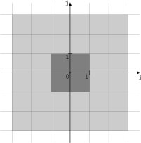
Figure 2: “Black” and “gray” regions of a ball of radius 3 centered at the origin

3.4 Construction for the case $k=2$

Suppose that $k=2$. Let $i$ and $j$ denote the two elements of $\mathcal{B}$.

3.4.1 Construction outline

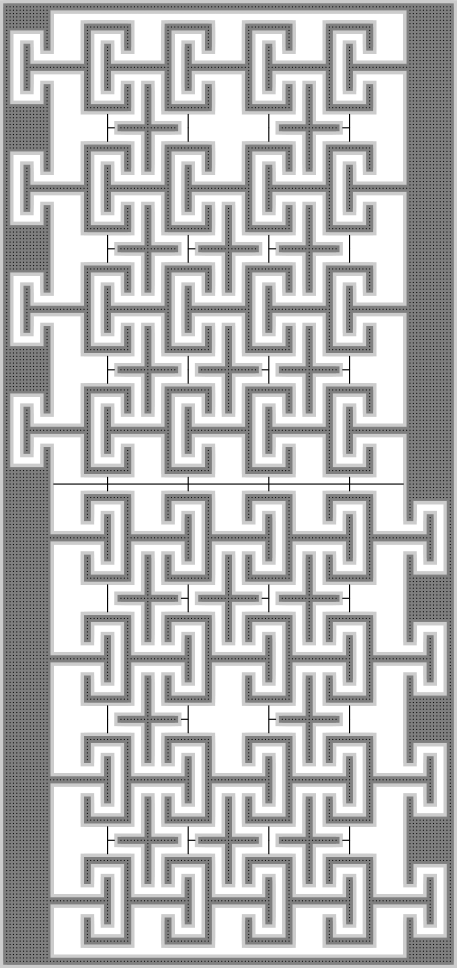
Figure 3: Schematic picture of the graph $X$ constructed by the logic engine pictured on Fig. 1. Bold dots denote balls’ centers, line segments denote auxiliary chain edges.

Let numbers $a_{ijk}$ describe a logic engine with $n$ rods and $m$ flag levels. We will construct a graph $X$ such that $X$ is (strictly/non-strictly) injectively embeddable in $\mathbb{R}^{1}$ if and only if the logic engine is realizable. As we said before, the construction will consist of bundles of balls of radius $r$ and auxiliary edge chains between them.

The skeleton $\Theta$ will consist of a frame $O$ and an axle $C$. The frame $O$ is a bundle of balls centered at integer points of the rectangular border $[0;W]\times[-H;H]$ (with parameters $W$ and $H$ to be chosen later). We will later modify $O$ by adding docking components (see below) as shown on Figure 3. The axle $C$ is a path $(0,0)$, $(1,0)$, …, $(W,0)$. Finally, $\Theta$ is induced by $V(O)\cup V(C)$.

Next, each of the $n$ rods of the logic engine will be represented by two chains anchored at the same point on the axle. Each chain consists of $m+1$ links. Each link is a bundle of balls centered at integer points of the rectangle $[0,w]\times[0,h]$ with addition of docking components (parameters $w$ and $h$ will be chosen later as well). We add edge chains of certain length to connect adjacent links, as well as the first link in the chain with the anchor point on the axle.

Finally, we attach flags to each chain according to flags positions in the logic engine. Each of the flags is a ball bundle with centers in integer points of the “cross”

$$\{(x,0)\mid x\in[-w_{f};w_{f}]\}\cup\{(0,y)\mid y\in[-h_{f};h_{f}]\}.$$

Flags can be attached at $m$ possible locations at midpoints of edge chains between adjacent links. Each flag points to the left or to the right in any embedding. Flags’ positions satisfy two rules:

• no flag can point “into the wall”,

• if two flags are attached on the same level on adjacent chains, then in any injective embedding such that their chains are on the same side on the axle, the flags must not point towards each other.

All the restrictions described above guarantee that injective embeddability of the constructed graph $X$ is equivalent to realizability of the logic engine.

In what follows we describe all parts of the construction in detail, and also provide a way to choose parameters $W$, $H$, $w$, $h$, $w_{f}$, $h_{f}$ so that injective embeddings of $X$ behave as expected. We will write $O(1)$ for any value with absolute value bounded by a constant independent of $n$ and $m$ (in particular, note that $r=O(1)$). Also, we will write $c_{i}$ for certain constants when explicit value is unimportant.

3.4.2 Link-axle and link-link connections

Let $\varphi$ be any injective embedding of the graph $X$ in $\Gamma$, and $T$ be the affine automorphism of $\Gamma$ induced by the restriction $\varphi|_{O}$ by Corollary 2.4.1. Then $T^{-1}\varphi$ must also be an injective embedding of $X$, hence we can assume that $T\equiv 1$, and $\varphi$ acts identically on $O$. Furthermore, $\varphi$ must also act identically on $C$; indeed, all edges of $C$ correspond to the primary direction $i$, hence there is a unique shortest path between $(0,0)$ and $(W,0)$, and $\varphi$ must preserve its vertices.

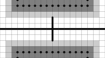
(a) $j\pm i\not\in\mathcal{A}$ case

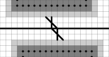
(b) $j-i\in\mathcal{A}$ case

Figure 4: Link-axle connection

Consider the connection between a link of width $w$ and the axle via an auxiliary two-edge chain. To ensure possibility of a strict embedding, the structure of the joint will depend on whether the elements $j\pm i$ belong to $\mathcal{A}$ (note that $j+i$ and $j-i$ cannot belong to $\mathcal{A}$ simultaneously since that would imply that $j$ is not a vertex of $\mathrm{Conv}\,\mathcal{A}$ and, therefore, not primary). Fig. 4 depicts two possible link-axle joints along with their embeddings (the $j+i\in\mathcal{A}$ case is symmetrical to the (b) case). Note that in both cases the embeddings are locally induced, that is, there are no hidden edges between the axle and the edge chain. We also have to add all possible edges between the link and the chain vertices. Note that these edges can only be incident to the midpoint of the chain since we have $||x||\leqslant 1$ for all $x\in\mathcal{A}$.

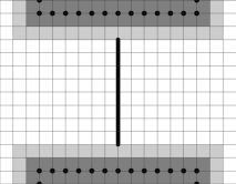
(a) Link-link connection (when $j\pm i\not\in\mathcal{A}$)

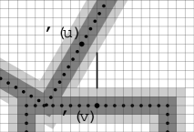
(b) Obstructed embedding of adjacent links in the $i_{1}\neq\pm i_{2}$ case after increasing $w$

Figure 5: Link-link connection

Adjacent links will be connected via edge chains of length $l=2r+4$ in a similar fashion. Let us show that it is possible to choose $w$ in such a way that in any injective embedding the horizontal edges of all chains are parallel to each other.

Suppose that $L_{1}$ and $L_{2}$ are adjacent links in a chain, and the link chain is located to the top of the axle (the situation is completely symmetrical at the bottom). Let $\varphi_{1}$ and $\varphi_{2}$ be the affine automorphisms of $\Gamma$ defined by restrictions of $\varphi$ to $L_{1}$ and $L_{2}$ respectively. Suppose that $\varphi_{1}$ and $\varphi_{2}$ map the vector (not the point!) $i$ to vectors $i_{1}$ and $i_{2}$ respectively, furthermore, suppose that $i_{1}\neq\pm i_{2}$. Since $i_{1}$ and $i_{2}$ are primary directions, they must be vertices of $\mathrm{Conv}\,\mathcal{A}$, thus $i_{1}\neq\pm i_{2}$ must imply that $i_{1}$ and $i_{2}$ are not parallel.

Consider the ball centers $u_{t}=u+ti$ of the “top edge” of $L_{1}$, and ball centers $v_{t}=v+ti$ of the “bottom edge” of $L_{2}$, where $t$ is an integer parameter that ranges within $[-w;w]$ (see Fig. 5(b)). Their images under the embedding $\varphi$ lie on two non-parallel lines $\varphi(u)+ti_{1}$ and $\varphi(v)+ti_{2}$. Let us find the intersection point of these lines: $\varphi(u)+t_{1}i_{1}=\varphi(v)+t_{2}i_{2}$, with $t_{1}$, $t_{2}$ not necessarily integer. Next, we can find integer $t^{\prime}_{1}$ and $t^{\prime}_{2}$ near $t_{1}$ and $t_{2}$ respectively, such that $||\varphi(u_{t^{\prime}_{1}})-\varphi(v_{t^{\prime}_{2}})||\leqslant 1$. If we introduce the requirement $w>\max(|t^{\prime}_{1}|,|t^{\prime}_{2}|)$, then the black regions of balls centered at $\varphi(u_{t^{\prime}_{1}})$ and $\varphi(v_{t^{\prime}_{2}})$ must intersect, hence this injective embedding becomes forbidden.

Finally, note that we must have $||\varphi(v)-\varphi(u)||\leqslant l$, hence $\max(|t^{\prime}_{1}|,|t^{\prime}_{2}|)<l\alpha$, where $\alpha=\alpha(i_{1},i_{2})$ depends only on $i_{1}$ and $i_{2}$. That is, to forbid injective embeddings with $i_{1}\neq\pm i_{2}$ it suffices to require $w>l\alpha_{max}$, where $\alpha_{max}$ is the maximal value of $\alpha(i_{1},i_{2})$ among all pairs $i_{1},i_{2}\in\mathcal{A}^{\prime}$ with $i_{1}\neq\pm i_{2}$. Since $l=O(1)$, the obtained requirement can be written as

$$w>c_{0}.$$ (1)

A similar reasoning applied to the link-axle connection implies that in any injective embedding with $i_{1}\neq\pm i$ the bottom edge of the first link will be obstructed by the axle vertices, therefore we must have $i_{1}=\pm i$. Hence, under requirement (1) all horizontal edges of all links must preserve their orientation. Let us note that we haven’t yet ensured that horizontal edges can’t have opposite directions, that is, the $i_{1}=-i_{2}$ case is not ruled out yet.

Let us choose the distance $\delta$ between adjacent link-axle connection points to be equal to $w+4r+4=w+O(1)$. Further, let the distance from the extreme link-axle connection points and the frame vertices be at least $\delta/2$, then it is possible to place the links without colliding with the frame. Put $W=(n+2)\delta$, then a rectangle of width $W$ fits all $n$ links as well as docking components (see Fig. 3). Similarly to the choice of $w$, we can show that it is possible to choose large enough

$$h>\beta W,$$ (2)

such that in any embedding all vertical edges of all links are vertical or collide with the frame.

Furthermore, let us choose $H$ so that to fit all link chains inside the frame vertically. It can be verified that the height of the top link’s gray region is at most $2+h+2r$ (height of the gray region of the bottom link) + $m\times(h+l+2r)$ (vertical translations between adjacent links). Putting $H=2+h+2r+m(h+l+2r)+r+2$, we guarantee that the distance between gray regions of the top side of the frame and the top link is at least 2. Clearly, $H=O(mh)$.

3.4.3 Docking components

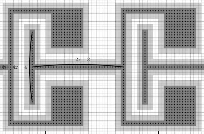
Figure 6: Docking component

For the construction to behave properly under possible embeddings, we must ensure that adjacent flags on the same level and side (relative to the axle) are located at close height in any embedding. However, we have “flexible” connections between adjacent links in a chain, thus there can be a significant discrepancy in height of neighbouring links and flags. Moreover, these discrepancies can add up without a limit since the number of levels $m$ is unbounded. We will introduce docking components in each of the links and in the frame to ensure that the height discrepancy of adjacent links stays bounded.

Consider a pair of adjacent links located on the same level to the top of the axle. Let us modify each of the links by expanding the bundles with extra ball centers lying on a forked T-shaped “antenna” (see Fig. 6). Further, let us make a “receiver” in each of the links by removing all balls with gray region within distance 1 of the gray region of the adjacent link’s antenna. We will choose dimensions of antennas as large as possible so that a link remains connected after making a suitable receiver.

As shown above, in any injective embedding all links must preserve orientation under requirements (1) and (2). Our intention is that in any embedding each pair of neighbouring links must be interlocked, that is, each antenna must be inside the corresponding receiver.

For a pair of neighbouring links $L_{1}$ and $L_{2}$ to the top of the axle let us consider vertices $u_{1}$, $v_{1}$, $u_{2}$, $v_{2}$ (see Fig. 7) that are the endpoints of the chains connecting $L_{1}$ and $L_{2}$ with the axle or with a previous link; in the latter case we will assume that the previous links are interlocked. We can verify that in any case $\varphi(v_{2})-\varphi(v_{1})=(\delta+O(1),O(1))$ holds.

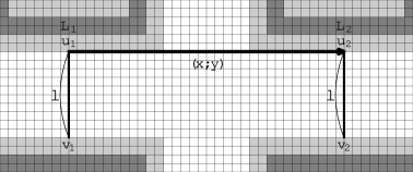
Figure 7: Edge chains connecting adjacent link pairs

First, suppose that the horizontal edges of $L_{1}$ and $L_{2}$ have the same direction, in that case we must have $\varphi(L_{2})=\varphi(L_{1})+(x,y)$. If $L_{1}$ and $L_{2}$ are not interlocked in $\varphi$, then we have either $x>\delta+w+c_{1}$ or $|y|>h+c_{2}$. But

$$(x,y)=\varphi(u_{2})-\varphi(u_{1})=(\varphi(u_{2})-\varphi(v_{2}))-(\varphi(u_{1})-\varphi(v_{1}))+(\delta+O(1),O(1)).$$

Note that $u_{1}$ and $v_{1}$ are connected by a path of length $l$; the same holds for vertices $u_{2}$ and $v_{2}$. Consequently, $x\leqslant 2l+\delta+c_{3}$ and $|y|<2l+c_{4}$. Let us enforce the inequalities $2l+\delta+c_{3}<\delta+w+c_{1}$ and $2l+c_{4}<h+c_{2}$ by increasing $w$ and $h$ (if necessary), so that none of the cases corresponding to non-interlocked links $L_{1}$ and $L_{2}$ are possible. Since $l=O(1)$, the two restrictions can be written as

$$w>c_{5},h>c_{6}$$ (3)

Under these restrictions, $L_{1}$ and $L_{2}$ must be interlocked. An inductive argument implies that all corresponding pairs of links will be interlocked (the situation is symmetrical to the bottom of the axle).

Finally, we must consider a situation when horizontal edges of links may have opposite direcion. In this case, we must have two links (or a link and a frame-attached docking component) with antennas pointing towards each other. Following the notation of the previous paragraph, in this case we must have either $x>2w+c^{\prime}$ or $|y|>h/2+c^{\prime\prime}$ for certain constants$\leavevmode\nobreak\ c^{\prime},c^{\prime\prime}$. This situation can be eradicated by strenghtening the requirement (3) if necessary.

Let us note that the shift between any pair of adjacent links in a chain (to the top of the axle) is $(O(1),h+O(1))$ since they are connected by a path of length $l=O(1)$.

3.4.4 Flags and attachments

A flag is attached to the midpoint of an auxiliary edge chain between consecutive links as shown on Fig. 8 (similarly to the situation on Fig. 4, several ways of attachment are possible). Let us choose the dimensions of a flag: $2w_{f}=\delta-2r-4=w+O(1)$, and $2h_{f}=h$.

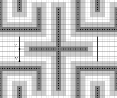
Figure 8: A flag and its attachment to an auxiliary edge chain

The length of the $uv$-path is $O(1)$, and the flag is connected to the vertex $u$ by a chain of two edges. We have shown above that the shift between two adjacent links on the same level is $(\delta+O(1),O(1))$, and the shift between consecutive links on a same chain is $(O(1),h+O(1))$. A reasoning similar to the one in Section 3.4.2 can show that under restrictions

$$w_{f}>c_{7},h_{f}>c_{8}$$ (4)

bars of the cross will be aligned with the axes in any embedding.

Let us ensure that two adjacent flags on the same level can not point towards each other. Let us enforce

$$2h_{f}>l+2r.$$ (5)

Now the vertical bar can not fit into the vertical gap between two links on the same chain, hence it has to be located in the space between the chains. But for this space to accomodate two crosses simultaneously, the gap must be at least $w_{f}$ wide; however, it is only $\delta-w+O(1)=O(1)$ wide. From this, we obtain the restriction:

$$w_{f}>c_{9}.$$ (6)

Finally, if a flag is pointed towards the wall of the frame, then we must have $\delta/2>w_{f}+O(1)$, which is equivalent to $w/2<O(1)$, hence we obtain the final requirement

$$w>c_{10}.$$ (7)

3.4.5 Choosing the parameters

It suffices now to choose suitable values for parameters $w$, $h$, $W$, $H$, $w_{f}$, $h_{f}$ to satisfy the restrictions (1)-(7), since we have established all necessary features of the construction required to implement the correct logic engine behaviour. It can be verified that we can choose $w=O(1)$, $h=O(n)$. We now have that all vertices of the graph $X$ fit inside a rectangle of dimensions $O(n)\times O(nm)$ in the basis $\mathcal{B}$. Vertices of $G$ are placed discretely in $\mathcal{B}$, hence the graph $X$ has size $O(n^{2}m)$.

Thus, the construction of the graph $X$ is a valid polynomial reduction from LOGIC-ENGINE to injective embeddability in $\mathbb{R}^{1}$, hence the latter is NP-hard.

3.4.6 Strict embeddability

Up to this point, we have only considered non-strict injective embeddings of $X$. However, note that if $X$ is injectively embeddable, then it must be strictly injectively embeddable as well. Indeed, let $\varphi$ denote an injective embedding of $X$ reconstructed from a logic engine realization in such a way that all auxiliary chains are aligned with corresponding axes (as on Fig. 3). It can be verified that in $\varphi$ the gray regions of different parts are at distance at least 2 apart, and $\varphi$ is locally induced in all chain attachment points, thus $\varphi(X)$ is an induced subgraph of $\Gamma$, consequently, $\varphi$ is strict. Thus, the reduction can be applied to strict injective embeddability just as well, and the complexity result is naturally extended.

Finally, to establish NP-hardness of strict non-injective embeddability, we invoke Prop. 1.3.2, and point out that no two vertices of $X$ have the same neighbourhood by construction of $X$. This concludes the proof of the (b) part of Theorem 1 in the $k=2$ case.

3.5 Construction for the $k>2$ case

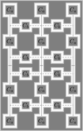
Figure 9: Construction scheme for the $k>2$ case. Dashed chains are introduced depending on whether a flag is present in the corresponding place of the logic engine.

As before, we choose $r=\max(R(\mathcal{A}),\max_{||x||\leqslant 1}\rho(x))$. For an integer $a$, let $C_{a}$ denote the ball bundle with centers in integer points of the hypercube region $S_{a}$.

The reduction of LOGIC-ENGINE to $\mathcal{A}$-embeddability in $\mathbb{R}^{1}$ for the $k>2$ case works as follows. Let the input logic engine contain $n$ rods, and $m$ flag levels on each side of the axle. Choose parameters $a$ and $b$. Construct the graph $X^{\prime}$ as a union of $2nm$ copies of the graph $C_{a}$ that emulate “chain links”, $2(n-1)m$ copies of $C_{b}$ that emulate flags, and auxiliary edge chains according to the Fig. 9. Here the horizontal direction corresponds to the axis $0b_{1}$, and the vertical direction to the axis $0b_{2}$, where $b_{1}$ and $b_{2}$ are elements of the basis $\mathcal{B}$ (all other elements of $\mathcal{B}$ are orthogonal to the displayed plane).

Choose $L$ as a large enough parallelepiped that encompasses $X^{\prime}$. We choose $L$ so that the set $L^{\prime}$ containing all integer points at least $r+2$ away (with respect to $l_{\infty}$ norm) of gray regions of balls of $X^{\prime}$ and auxiliary chains is connected in $\Gamma$. Construct a “framework” graph $Y$ as an induced union of balls with vertices in $L^{\prime}$. The black regions of balls of $Y$ contain $L$ with removed neighbourhoods of all $C_{a}$ and $C_{b}$, and “corridors” of width $2r+4$ around auxiliary chains. To obtain the graph $X$, attach all auxiliary chains along with the paths anchoring them to $Y$, and also attach the flags according to the input logic engine configuration.

As with the $k=2$ case, the restriction of any embedding of $X$ to the vertices of the ball bundle $Y$ is an affine automorphism of $\Gamma$, hence we can assume that any embedding of $X$ acts trivially on $Y$. We claim that for $a,b\geqslant D$ and large enough $D$ we have that in any embedding of $X$ all images of $C_{a}$ and $C_{b}$ must be aligned with coordinate axes.

Consider a copy of $C_{D}$, and assume that in any embedding of $X$ its image lies completely within $L$. First, observe that for a large enough $D$ the image of the center of $C_{D}$ cannot lie in any “corridor” of width $2r+4$. Indeed, the restriction of an embedding to vertices of $C_{D}$ is composed of a translation and a non-degenerate linear map $T:\mathbb{R}^{k}\to\mathbb{R}^{k}$ that is a unique extension of an element of $\mathrm{Aut}_{0}(\Gamma)$. For a particular $T$, choose $D$ so large that $T(S_{D})$ contains all points at most $r+3$ away from the cube center. We now have that the black region of $T(C_{D})$ cannot fit in any corridor by at least one dimension. FInally, observe that there are only finitely many options for $T$, hence we can choose $D$ that excludes placing $C_{D}$ in a corridor for each of the options.

Let the center of $C_{D}$ now lie an a cubic neighbourhood of size $D+2r+2$. Let $T$ denote the same linear map as in the previous paragraph. Observe that $T(\mathrm{Conv}\,\mathcal{A})=\mathrm{Conv}\,\mathcal{A}$, hence $T$ is volume-preserving (i.e. has Jacobian equal to $\pm 1$). Consider the bounding box (that is, the least enclosing axes-aligned parallelepiped) of the set $T(S_{D})$ denoted as $P_{D}$. Let $(p_{1}(D),\ldots,p_{k}(D))$ denote the linear dimensions of $P_{D}$. If $T(C_{D})\neq C_{D}$, then $p_{i}(D)>D$ for a certain coordinate $i$. Moreover, the numbers $p_{i}(D)$ are linear in $D$.

The faces of the cubic neighbourhoods in our construction are allowed to have “windows”, that is, openings of corridors of width $2r+4$. Let us show that image of a large enough $C_{D}$ does not fit in a cubic neighbourhood with windows. Let $H_{z}$ denote the hyperplane $x_{i}=z$ (with the index $i$ chosen above). Suppose that the center of the image of $C_{D}$ has coordinate $i$ equal to $x_{i}$ relative to the center of the cubic neighbourhood. Then we must have both

$$\mathrm{Vol}_{k-1}(T(S_{D})\cap H_{D+r+1-x_{i}})\leqslant(2r+4)^{k-1},\mathrm{Vol}_{k-1}(T(S_{D})\cap H_{D+r+1+x_{i}})\leqslant(2r+4)^{k-1},$$

since otherwise the black region of $T(C_{D})$ does not fit into the windows of $(k-1)$-dimensional volume $(2r+4)^{k-1}$. The value $\min(\mathrm{Vol}_{k-1}(T(S_{D})\cap H_{D+r+1\pm x_{i}}))$ is attained for $x_{i}=0$, so it suffices to show

$$\mathrm{Vol}_{k-1}(T(S_{D})\cap H_{D+r+1})>(2r+4)^{k-1}$$

for sufficiently large $D$.

Let $q$ be the point of $T(S_{1})$ with the largest coordinate $i$, and $t=p_{i}(1)>1$ be the value of this coordinate. The $(k-1)$-dimensional volume $\mathrm{Vol}_{k-1}(T(S_{1})\cap H_{1})=z_{1}$ must be positive. We have that $\mathrm{Vol}_{k-1}(T(S_{D})\cap H_{D})=z_{1}D^{k-1}$. Further, by convexity the set $T(S_{D})\cap H_{D+r+1}$ must contain the homothetical image of $T(S_{D})\cap H_{D}$ with the homothetic center $Dq$ and coefficient $(Dt-(D+r+1))/(Dt-D)$, hence

$$\mathrm{Vol}_{k-1}(T(S_{D})\cap H_{D+r+1})\geqslant z_{1}D^{k-1}\cdot\left(\frac{Dt-(D+r+1)}{Dt-D}\right)^{k-1}=z_{1}D^{k-1}\left(1-\frac{r+1}{D(t-1)}\right)^{k-1}$$

Clearly, the right-hand side can be made larger than $(2r+4)^{k-1}=O(1)$ by choosing a large enough $D$. It follows that $T(C_{D})=C_{D}$ in any embedding for a large enough $D$.

Let us now choose suitable values for $a$ and $b$. Let $a,b\geqslant D$ and $a>b+2r+2$, then in any embedding images of all copies of $C_{a}$ and $C_{b}$ must be axes-aligned, and also copies of $C_{a}$ cannot fit into neighbourhoods of $C_{b}$. Let us further impose $2(2a)^{k}>(2a+2r+2)^{k}$, $2(2b)^{k}>(2b+2r+2)^{k}$, $(2a)^{k}+(2b)^{k}>(2a+2r+2)^{k}$. Under these restrictions no two cube copies cannot lie within the same neighbourhood due to natural volume inequalities. Finally, due to distance limitations imposed by the auxiliary edge chains, the chain links will be positioned vertically, and each flag can only go to the slot nearest to the anchoring point. It follows that each copy of $C_{a}$ will lie in a neighbourhood of size $a+2r+2$, hence the copies of $C_{b}$ will lie in neighbouhoods of size $b+2r+2$. Consequently, we can restore a logic engine realization from any embedding of $X$. Finally, we are free to choose any suitable directions for link chains and flags, hence a logic engine realization can be turned to an embedding of $X$. In this way, the two problems are seen to be equivalent.

Since the chosen $a$ and $b$ are independent on the input, we have $a=O(1)$, $b=O(1)$, and the graph $X$ is enclosed in a parallelepiped with dimensions $O(n)\times O(m)\times O(1)\times\ldots\times O(1)$, and its size is $O(nm)$. Thus the reduction from LOGIC-ENGINE is polynomial, and the (b) case of Theorem 1 is established for injective embeddings.

To conclude the proof of Theorem 1 we consider strict non-injective $\mathcal{A}$-embeddings for $k>1$. It can be verified explicitly that the reduction graphs constructed in Sections 3.4 and 3.5 do not have vertices with equal neighbourhoods. Consequently, Proposition 1.3.2 implies that each of these graphs is strictly $\mathcal{A}$-embeddable if and only if it is strictly injectively $\mathcal{A}$-embeddable, hence the same constructions work for reducing LOGIC-ENGINE to the strict embeddability problem. Theorem 1 is now proven completely.

References

- [1] P Erdős “On Sets of Distances of Points” In American Mathematical Monthly JSTOR, 1946, pp. 248–250
- [2] Andrei Mikhailovich Raigorodskii “Borsuk’s problem and the chromatic numbers of some metric spaces” In Russian Mathematical Surveys 56.1 IOP Publishing, 2001, pp. 103
- [3] Peter Brass, William OJ Moser and János Pach “Research problems in discrete geometry” Springer, 2005
- [4] Andrei M Raigorodskii “Coloring distance graphs and graphs of diameters” In Thirty Essays on Geometric Graph Theory Springer, 2013, pp. 429–460
- [5] Andrei M Raigorodskii “Cliques and cycles in distance graphs and graphs of diameters” In Discrete Geometry and Algebraic Combinatorics 625 American Mathematical Society, 2014, pp. 93–110
- [6] Andrei M Raigorodskii “Combinatorial geometry and coding theory” In Fundamenta Informaticae 145.3 IOS press, 2016, pp. 359–369
- [7] AB Kupavskii “The chromatic number of with a set of forbidden distances” In Doklady Mathematics 82.3, 2010, pp. 963–966 Springer
- [8] Elena S Gorskaya, Irina M Mitricheva, Vladimir Yu Protasov and Andrei M Raigorodskii “Estimating the chromatic numbers of Euclidean space by convex minimization methods” In Sbornik: Mathematics 200.6 IOP Publishing, 2009, pp. 783
- [9] Marcus Schaefer “Realizability of graphs and linkages” In Thirty Essays on Geometric Graph Theory Springer, 2013, pp. 461–482
- [10] James B Saxe “Embeddability of weighted graphs in -space is strongly NP-hard” In Proc. 17th Allerton Conf. Commun. Control Comput, 1979, pp. 480–489
- [11] Boris Horvat, Jan Kratochvíl and Tomaž Pisanski “On the computational complexity of degenerate unit distance representations of graphs” In Combinatorial algorithms Springer, 2011, pp. 274–285
- [12] Mikhail Tikhomirov “On computational complexity of length embeddability of graphs” In Discrete Mathematics 339.11 Elsevier, 2016, pp. 2605–2612
- [13] Kellogg S Booth and George S Lueker “Testing for the consecutive ones property, interval graphs, and graph planarity using PQ-tree algorithms” In Journal of Computer and System Sciences 13.3 Elsevier, 1976, pp. 335–379
- [14] Peter J Looges and Stephan Olariu “Optimal greedy algorithms for indifference graphs” In Computers & Mathematics with Applications 25.7 Elsevier, 1993, pp. 15–25
- [15] Heinz Breu and David G Kirkpatrick “Unit disk graph recognition is NP-hard” In Computational Geometry 9.1 Elsevier, 1998, pp. 3–24
- [16] Ross J Kang and Tobias Müller “Sphere and dot product representations of graphs” In Discrete & Computational Geometry 47.3 Springer, 2012, pp. 548–568
- [17] Petr Hliněný and Jan Kratochvíl “Representing graphs by disks and balls (a survey of recognition-complexity results)” In Discrete Mathematics 229.1 Elsevier, 2001, pp. 101–124
- [18] Gary MacGillivray “Graph homomorphisms with infinite targets” In Discrete Applied Mathematics 54.1 Elsevier, 1994, pp. 29–35
- [19] Jiřı́ Matoušek and Robin Thomas “On the complexity of finding iso-and other morphisms for partial k-trees” In Discrete Mathematics 108.1 Elsevier, 1992, pp. 343–364
- [20] Hans L Bodlaender “A tourist guide through treewidth” In Acta cybernetica 11.1-2, 1994, pp. 1
- [21] Aleksandr Andreevich Ryabchenko “Isomorphisms of Cayley graphs of a free abelian group” In Siberian Mathematical Journal 48.5 Springer, 2007, pp. 919–922
- [22] Peter Eades and Sue Whitesides “The logic engine and the realization problem for nearest neighbor graphs” In Theoretical Computer Science 169.1 Elsevier, 1996, pp. 23–37
- [23] Sandeep N Bhatt and Stavros S Cosmadakis “The complexity of minimizing wire lengths in VLSI layouts” In Information Processing Letters 25.4 Elsevier, 1987, pp. 263–267
- [24] Angelo Gregori “Unit-length embedding of binary trees on a square grid” In Information Processing Letters 31.4 Elsevier, 1989, pp. 167–173
- [25] Peter Eades and Sue Whitesides “The realization problem for Euclidean minimum spanning trees is NP-hard” In Algorithmica 16.1 Springer, 1996, pp. 60–82
- [26] Sándor P Fekete, Michael E Houle and Sue Whitesides “The wobbly logic engine: Proving hardness of non-rigid geometric graph representation problems” In International Symposium on Graph Drawing, 1997, pp. 272–283 Springer
- [27] Matthew Kitching and Sue Whitesides “The three dimensional logic engine” In International Symposium on Graph Drawing, 2004, pp. 329–339 Springer