Mean Field Game Approach to Production and Exploration of Exhaustible Commodities

Abstract

In a game theoretic framework, we study energy markets with a continuum of homogenous producers who produce energy from an exhaustible resource such as oil. Each producer simultaneously optimizes production rate that drives her revenues, as well as exploration effort to replenish her reserves. This exploration activity is modeled through a controlled point process that leads to stochastic increments to reserves level. The producers interact with each other through the market price that depends on the aggregate production. We employ a mean field game approach to solve for a Markov Nash equilibrium and develop numerical schemes to solve the resulting system of non-local HJB and transport equations with non-local coupling. A time-stationary formulation is also explored, as well as the fluid limit where exploration becomes deterministic.

Keywords: mean field games, exhaustible resources, dynamic Cournot models.

1 Introduction

We consider a stochastic differential game model for an exhaustible commodity market, such as oil. The dynamic market evolution is driven by the use of existing reserves to produce energy and exploration/discovery of new reserves. We assume a Cournot-type competition where each producer chooses their production rate; this resembles e.g. OPEC members who adjust their output to influence crude oil prices. Extraction of the commodity generates a revenue stream but carries the depletion trade-off. To offset the resulting lower reserves, producers undertake efforts to explore for new reserves. Exploration is uncertain: continuous exploration efforts stochastically lead to discrete discoveries of additional reserves. Individually, producers aim to maximize their total expected profits which are equal to price times quantity extracted, minus the production and exploration costs. Strategically, the producers interact via the global market price $p$ that is determined by the aggregate production.

To model this oligopoly among commodity producers (i.e. energy firms), we assume a continuum of homogenous agents who compete in a single market for energy. Each agent is small enough to be a price taker, yet in equilibrium the aggregate behavior fully determines supply and in turn the clearing price. For simplicity, we assume constant demand, focusing on producers’ choices. This model is reasonable to describe the long-term behavior of the market (on the scale of years), where micro-economic fluctuations are averaged out and commodity supply and reserves is the main determinant of market structure.

While the literature on single-agent optimization for exhaustible resource extraction dates back to the 1970’s [14, 27, 28], the first rigorous treatment of a dynamic continuous-time non-cooperative model was by Harris et al. [22] in 2010. They studied an $N-$player Cournot game via the associated system of nonlinear HJB partial differential equations but due to numerical challenges illustrations were limited to the two-player model. Further analysis of competitive duopoly was carried out in [25] and our earlier work [26]; the special case of a single exhaustible player competing against $N$ renewable producers of varying profitability was studied in [24, 13].

1.1 Mean field game approach

In a differential game model with a finite number $N$ of players, their equilibrium strategies can be determined by a system of Hamilton-Jacobi-Bellman-Isaacs (HJB-I) equations derived from the dynamic programming principle. The dimension of the system in general increases in $N$, which makes the game model intractable for large $N$. Mean field game (MFG) approach simplifies the modeling by considering equilibria with a continuum of homogenous players; the respective finite dimensional game state expands into a distribution $m(\cdot)$. The main idea is then to consider the optimization problem of the representative agent; the latter becomes a regular stochastic control problem with the competitive effect captured via a mean-field interaction driven by $m(\cdot)$. In turn, the aggregate behavior of the players implies dynamics on the distribution $m$ of agent states. This leads to a system of two partial differential equations (PDE’s) which is viewed as an approximation to a single multi-dimensional HJB-I PDE in the original finite-$N$ setup. We refer to [4, 9] for the general theory of MFGs.

In our context, the individual states are the reserves’ levels $X$, and the interaction is via the market price $p$ that is related to total production $Q$ across all the producers. Thus, $p$ enters the game value function of the representative producer as the mean field term and drives her choice of production and exploration controls. In turn, the distribution of reserves is driven by the latter production rates and exploration efforts. The key aspect of such oligopolistic MFG’s, first introduced in Guéant’s PhD thesis [19, 20], is the mean-field interaction via the aggregate $Q$. Since producers directly optimize their own production rates, this corresponds to a mean-field game of controls, in contrast to the standard situation where the interaction is through the density $m(\cdot)$. A second distinguishing feature of Cournot MFG’s is the hard exhaustibility constraint when reserves reach zero. Different possibilities at $X_{t}=0$ include leaving the game (which magnifies market power of remaining producers); switching to a renewable/inexhaustible resource; prolonging production via costly reserve replenishment. All the above choices lead to non-standard boundary conditions in the respective equations, necessitating tailored treatment.

Two further crucial aspects of oligopoly MFG concern the prescribed dynamics of the reserves process $(X_{t})$ and the inverse demand curve that relates $p$ to aggregate production $Q$. For the latter aspect, starting with [20], price was assumed to be linear (decreasing) in quantity, which brings forward some of the tractability of the original linear-quadratic MFG’s. This choice was maintained in [11, 16, 17]. Very recently, Chan and Sircar [12] also investigated MFG’s with power-type demand curves. We note that even with linear price schedule, the overall link between production and price is non-linear due to the exhaustibility condition at $x=0$ which requires to separately keep track of exhausted and producing firms.

For an exhaustible resource, reserves are non-increasing and are completely determined by past production. However, this does not capture the real-life aspect of replenishment of fossil-fuel commodities, where global reserve depletion has to a large degree been offset with ongoing discoveries (deep-sea oil, shale gas, oil sands, and so on). Such discoveries take place thanks to exploration activities determined by the respective exploration efforts. In the early model of Pindyck [27], exploration was incremental, leading to deterministic reserve additions. Subsequent extensions represented exploration as a point process counting new reserve discoveries, see [3, 15, 21] which is also the choice we pursue below. Another alternative, which is motivated by uncertainty about current reserves, has been to introduce exogenous Brownian noise, i.e. make reserves stochastically fluctuating. This is also convenient for theoretical and numerical purposes and has been commonly used in recent MFG literature, see [11, 17, 18, 20]. Let us also mention further possibilities of $(X_{t})$ following a stochastic differential equation with controlled volatility and drift [28] and a common noise MFG model to capture systematic shocks to aggregate reserves [16].

Mathematically, the MFG setup leads to an HJB equation to model a representative agent’s strategy, and a transport equation to model the evolution of the distribution of all the producers’ states. The structure of these equations is determined by the prescribed dynamics of $(X_{t})$. When $X_{t}$ is deterministic, the equations are first-order, see e.g. [5]. When $X_{t}$ includes Brownian shocks (cf. [20, 11]), the HJB equation is second-order and the transport equation is the usual Kolmogorov forward equation. In contra-distinction, discrete discoveries add a first-order non-local (“delay”) term to both the HJB [25, 26] and transport equations. These features are central to the numerical resolution of MFG’s that requires handling a coupled system of nonlinear PDE’s. We refer to [1, 2, 8] for a general summary of different computational approaches and their convergence, including finite difference and semi-Langrangian schemes. An alternative common approach [20, 11, 12] is based on Picard-like iterative schemes.

1.2 Summary of Contributions

In this paper we apply the MFG approach to model energy markets with a large population of competing producers of exhaustible but replenishable resources. Our main focus is the strategic interaction between exploration and production (E&P), in a dynamic, stochastic, game-theoretic framework. E&P is a major theme in the business decisions of energy firms, but is rarely tackled as such in mathematical models. Some of the topics we investigate are: (i) the price effect of exploration; (ii) aggregate production path implied by the model; (iii) aggregate exploration efforts; (iv) possibility of a stationary equilibrium where exploration exactly offsets production; (v) impact of exploration uncertainty on the solution. Our analysis yields quantitative insights into the macro behavior of commodity industries on long-time horizons, linking up with colloquial topics of “peak oil”, “value of exploration R&D” and “postponing the exhaustion Doomsday”. Specifically, the stationary model where individual resource levels stochastically change, but the overall reserves distribution and associated aggregate production and price remain constant, is a feature that to our knowledge is new in the oligopoly MFG literature.

Relative to existing Cournot MFG models, we emphasize the analysis of stochastic exploration which leads to first-order, non-local MFG equations. In that sense, our work fits into two different strands of game-theoretic models of energy production. On the one hand, we extend [11, 20] who considered exhaustible resource MFGs but without exploration; thus reserves were non-increasing. On the other hand, we extend the duopoly model [25] to the limiting oligopoly with a continuum of producers. In the duopoly each producer directly influences the price; in the MFG model herein, each producer has negligible power on market price that is rather driven by the aggregate production.

The closest work to ours is by Chan and Sircar [12] who primarily focused on competition of exhaustible producers who switch to a costly renewable resource upon ultimate depletion. They also studied competition of a large group of exhaustible producers alongside a single renewable producer, similar to the major-minor model of Huang [23]. Section 5 of [12] then briefly discusses resource exploration and the respective stationary equilibrium. Compared to their illustration, we provide multiple additional analyses, including a detailed treatment of both the time-dependent and time-stationary equilibria, convergence to stationarity as the problem horizon increases, and study of the “fluid limit”. The latter is a law-of-large-numbers scaling that maintains exploration/production controls but removes the associated uncertainty. This mechanism allows to quantify the pure impact of uncertainty on the MFG model, linking to the deterministic first-order MFG, which is another new development relative to existing literature.

Our setup generates several numerical challenges due to the non-local terms in the PDE’s and a non-local coupling between them; a major part of the paper is devoted to constructing a computational scheme to solve the MFG equations. Specifically, we decouple the HJB and transport equations via a Picard-like iteration that alternately updates the optimal production and exploration controls, and the reserves distribution function (which in turn determines the market price). For the HJB equation and similar to [12], we employ a method of lines, discretizing the space dimension and solving the resulting ordinary differential equations in the time dimension. The latter still constitutes a coupled system of ODE’s due to the exploration control and the implicit boundary condition at $x=0$. For the transport equation we use a fully explicit finite-difference scheme. However, due to the non-smooth dynamics of $(X_{t})$, rather than working with the density $m(dx)$, we operate with the corresponding cumulative distribution function $\eta(\cdot)$, and moreover separately treat the proportion $\pi(t)$ of exhausted producers.

This paper is organized as follows. In Section 2, we introduce the $N$-player Cournot game that motivates the MFG model in the limit $N\rightarrow\infty$. Section 3 discusses the doubly coupled system of HJB and transport equations that characterize the MFG Nash equilibrium. Section 4 is devoted to numerical methods for solving this system and presents numerical illustrations. The rest of the paper then presents two modifications of the main model that yield important economic insights. In Section 5, we study the stationary MFG model, in which the reserves distribution remains invariant due to the counteracting effects of production and exploration. Section 6 investigates the asymptotic “fluid limit” regime whereby the exploration process becomes deterministic, so that discovery of new resources happens at high frequency with infinitesimal discovery amounts. The paper concludes with Section 7 and an Appendix that contains most of the proofs.

2 Model

2.1 Finite player Cournot game

We consider an energy market with $N$ producers (players). Each producer uses exhaustible resources, such as oil, to produce energy. Let $X^{i}_{t}$ represent the reserves level of player $i$, $i=1,\ldots,N$. Each $X^{i}_{t}$ takes values in the set $\mathds{R}_{+}$ of nonnegative real numbers. Reserves level $X^{i}_{t}$ decreases at a controlled production rate $q^{i}_{t}\geq 0$, and also has random discrete increment due to exploration. We use a controlled point process $(N^{i}_{t})$ to model arrivals of new discoveries. Specifically, $N^{i}_{t}$ has intensity $\lambda(t)a^{i}_{t}$, where $a^{i}_{t}$ is the exploration effort controlled by player $i$. The parameter $\lambda(t)$ is rate of discovery per unit exploration effort which reflects the current exploration techniques and overall resources underground, it is thus taken as exogenously given and the same for all producers. Since total resources underground are depleted over time, it is reasonable to assume that $\lambda(t)$ is decreasing in $t$ and $\lim_{t\rightarrow\infty}\lambda(t)=0$. Let $\tau_{n}^{i}$ be the $n$-th arrival time of the point process $N_{t}^{i}$, then the inter-arrival time between the $n$-th and $(n+1)$-st arrivals satisfies the following probability distribution

$$\mathds{P}\left(\tau^{i}_{n+1}>\tau^{i}_{n}+t\right)=\exp\left(-\int_{\tau^{i}_{n}}^{\tau^{i}_{n}+t}\lambda(s)a^{i}_{s}ds\right).$$

Let $\delta$ denote the unit amount of a discovery, which is assumed to be a positive constant as in [25, 26]. The unit amount of discovery $\delta$ can be random in general, see Remark 3.1. The reserves dynamics of each player are given by the following stochastic differential equation

$$dX^{i}_{t} =-q^{i}_{t}\mathds{1}_{\{X^{i}_{t}>0\}}dt+\delta dN^{i}_{t},\quad i=1,2,\ldots,N,\qquad X^{i}_{0}=x^{i}_{0}\geq 0,$$ (2.1)

where $x^{i}_{0}$ is the initial reserves level. The indicator function $\mathds{1}_{\{X^{i}_{t}>0\}}$ means that production must be shut down, $q^{i}_{t}=0$, whenever reserves run out, $X^{i}_{t}=0$. With (2.1) reserves decrease continuously between discoveries according to the production schedule and experience an instantaneous jump of size $\delta$ at discovery epochs.

Cost functions. We assume that all producers have identical quadratic cost functions of production and exploration, denoted by $C_{q}(\cdot)$ and $C_{a}(\cdot)$ respectively,

$$C_{q}(q)=\kappa_{1}q+\beta_{1}\frac{q^{2}}{2},\qquad C_{a}(a)=\kappa_{2}a+\beta_{2}\frac{a^{2}}{2}.$$ (2.2)

The coefficients $\beta_{1,2}>0$ of the quadratic terms are assumed to be positive, making the cost functions strictly convex and guaranteeing that the optimal production and exploration effort levels are finite. The coefficients $\kappa_{1,2}\geq 0$ of the linear terms represent constant marginal cost of production and exploration due to the use of facilities and labor, while $\beta_{1},\beta_{2}$ of the quadratic terms represent increasing marginal costs due to negative externalities (such as rising labor costs or nonlinear taxation). We note that when $\kappa_{2}=0$ then exploration is always undertaken, otherwise $a^{\ast}_{t}=0$ could be optimal.

Supply-demand equilibrium. We assume there is a single market price $p$ (so the market is undifferentiated which is a reasonable assumption for the energy industry); in equilibrium $p$ is determined by equating the total demand to the total supply at that price level. This equilibrium is achieved instantaneously at each date $t$, which is viewed as fixed in the following exposition.

In addition to the $N$ producers we assume there are $M$ undifferentiated consumers. The demand of consumer $j$, denoted by $d^{j}$, depends on the price through the linear demand function $d^{j}=D(p)=L-p$. Note that demand is finite even at zero price and the demand elasticity is bounded. The aggregate demand, denoted by $Q^{(M)}_{demand}$, is the sum

$$Q^{(M)}_{demand}:=\sum_{j=1}^{M}d^{j}=M(L-p).$$

We now equate total demand with total supply $Q^{(N)}$ and substitute the right-hand-side above to obtain the equilibrium relation between total supply and price, $Q^{(N)}=M(L-p).$ Finally, the clearing price can be represented through the inverse demand function

$$p_{t}=L-\frac{1}{M}Q^{(N)}_{t}=L-\frac{N}{M}\left(\frac{1}{N}\sum_{i=1}^{N}q^{i}_{t}\right)=L-\frac{N}{M}\bar{Q}_{t},$$ (2.3)

where $\bar{Q}_{t}$ is the average production rate. To obtain a nontrivial limiting price as the number of producers and the number of consumers both go to infinity, we see that it is necessary to take $M\propto N$. Without loss of generality (if necessary by redefining $L$), we assume $M=N$, so that $p_{t}=L-\bar{Q}_{t}=D^{-1}(\bar{Q}_{t})$ where $L$ can be interpreted as the cap on prices as supply vanishes.

2.2 Game value functions and strategies

In a continuous-time Cournot game model, each player continuously chooses rate of production $q^{i}_{t}$ in order to maximize profit which is equal to the revenue $p_{t}\cdot q^{i}_{t}$, minus the production and exploration costs, integrated and discounted at a rate $r>0$. We work on a finite time horizon $[0,T]$, where $T$ is exogenously specified. The role of the horizon will be revisited in the sequel. The price $p_{t}$ each player receives is determined through the inverse demand function (2.3).

Denoting player-$i$’s strategy by $s^{i}:=\left(q^{i},a^{i}\right)$, the overall strategy profile for all the $N$ players is $\boldsymbol{s}:=\left(s^{1},s^{2},...,s^{N}\right)$. Starting with reserves state $\left(X^{1}_{t},\cdots,X^{N}_{t}\right)=:\bf{X}_{t}=\bf{x}$, each player’s objective functional $\mathcal{J}^{i},i=1,\ldots,N$ on the horizon $[t,T]$ is defined as the total discounted profit

$$\mathcal{J}^{i}\left(\boldsymbol{s};t,\bf{x}\right):=\mathbb{E}\left\{\int_{t}^{T}\left[D^{-1}\left(\frac{1}{N}\sum_{j=1}^{N}q^{j}_{s}\right)q_{s}^{i}-C_{q}(q_{s}^{i})-C_{a}(a_{s}^{i})\right]e^{-r(s-t)}\ ds\ \Big{|}\ \bf{X}_{t}=\bf{x}\right\},$$ (2.4)

where the expectation is over the random point processes $N^{j}$’s that drive $X^{j}$’s and hence $q^{j}$’s. We focus on the admissible set $\mathcal{A}$ of strategies whereby $s^{i}_{t}=(q^{i}_{t},a^{i}_{t})$ are Markovian feedback controls $q^{i}_{t}=q^{i}(t,{\bf X}_{t})$, $a^{i}_{t}=a^{i}(t,{\bf X}_{t})$ such that $\mathcal{J}^{i}({\bf{s}};t,\bf{x})<\infty$, $\forall{\bf{x}}\in\mathds{R}^{N}_{+}$, for all $i=1,\ldots,N$. From (2.4), we see that each player’s choice of strategy depends on the strategies of all the others, leading to a non-cooperative game. Our aim is to investigate the resulting (Markov feedback) Nash equilibrium. Importantly, the feedback structure of the controls together with (2.3) imply that player $i$’s dependence on $\bf{X}_{t}$ can be summarized by his individual reserves $X^{i}_{t}$ and the aggregate distribution of all players’ reserves. The latter is characterized through the upper-cumulative distribution function defined by

$$\eta^{(N)}(t,x):=\frac{1}{N}\sum_{j=1}^{N}\mathds{1}_{\left\{X^{j}_{t}\geq x\right\}}.$$

Thus the Markovian feedback controls $\left(q^{i},a^{i}\right)$ can be equivalently represented as

$$q^{i}_{t} =q^{i}\left(t,X^{i}_{t};\eta^{(N)}(t,\cdot)\right),\qquad a^{i}_{t}=a^{i}\left(t,X^{i}_{t};\eta^{(N)}(t,\cdot)\right),\qquad i=1,\ldots,N.$$

Definition 2.1 (Nash equilibrium).

A Nash equilibrium of the $N$-player game is a strategy profile $\boldsymbol{s}^{\ast}=\left(s^{1,\ast},\ldots,s^{N,\ast}\right)$, with $s^{i,\ast}:=\left(q^{i,\ast},a^{i,\ast}\right)$ such that

$$\mathcal{J}^{i}\left(\boldsymbol{s}^{\ast};t,\bf{x}\right)\geq\mathcal{J}^{i}\left((\boldsymbol{s}^{\ast,-i},s^{i});t,\bf{x}\right),\quad\forall i\in\{1,2,\ldots,N\},$$ (2.5)

where $(\boldsymbol{s}^{\ast,-i},s^{i})$ is the strategy profile $\boldsymbol{s}^{\ast}$ with the $i$-th entry replaced by arbitrary $s^{i}=(q^{i},a^{i})\in\mathcal{A}$.

In words, a Nash equilibrium is the set of strategies of the $N$ players such that no one can better off by unilaterally changing his own strategy. Theoretically the Nash equilibrium of the $N$-player game can be found by Hamilton-Jacobi-Isaacs (HJB-I) approach. HJB-I approach is to use dynamic programming principle to derive the partial differential equation of each player’s game value function, with other players’ strategies as entries. It is extremely hard to find a Nash equilibrium by using the (HJB-I) approach either analytically or numerically, even for small $N$, e.g. $N=2$. Thus in the following Section 2.3, we introduce the mean field game model as $N\rightarrow\infty$, which serves as an approximation to the Nash equilibrium of the game when number of players is very large.

2.3 Mean field game problem as $N\rightarrow\infty$

As the number of players becomes very large $N\rightarrow\infty$, thanks to the Law of Large Numbers, the empirical distribution $\eta^{(N)}$ is expected to converge to a CDF $\eta$. The limiting $\eta(t,x)$ is regarded as the reserves distribution among all players at date $t$, which means, for a given $t$ and $x$, the proportion of all players at time $t$ with reserves level greater than or equal to $x$. The production and exploration controls continue to take the Markovian feedback form

$$q_{t} =q(t,X_{t};\eta(t,\cdot)),\quad a_{t}=a(t,X_{t};\eta(t,\cdot)).$$ (2.6)

To re-solve for the supply-demand equilibrium clearing price, we use the total quantity $Q(t)$ of production at time $t$, defined as the Stieltjes integral of a representative producer’s production rate with respect to the reserves distribution,

$$Q(t):=-\int_{0}^{\infty}q(t,x;\eta)\ \eta(t,dx).$$ (2.7)

Note that $\eta(t,x)$ is decreasing in $x$, thus we add a negative sign to the integral in order to keep $Q(t)$ positive. The definition in (2.7) is the limit of the original $\bar{Q}_{t}$ that was defined for the $N$-player game. As before $Q(t)$ is linked to the clearing price via

$$p(t,\eta(t,\cdot))=D^{-1}(Q(t))=L+\int_{0}^{\infty}q(t,x;\eta)\ \eta(t,dx).$$ (2.8)

For a representative producer who starts with initial reserves level $X_{t}=x$ (with $x\in\mathbb{R}_{+}$ now a scalar), and representing all other players’ states via $\eta(\cdot,\cdot)$ taken as given, the mean-field objective functional is defined analogously to (2.4):

$$\mathcal{J}\left(q,a;t,x,\eta\right):=\mathbb{E}\left\{\int_{t}^{T}\left[p(s,\eta(s,\cdot))q_{s}-C_{q}(q_{s})-C_{a}(a_{s})\right]e^{-r(s-t)}\ ds\ \middle|X_{t}=x\right\}.$$ (2.9)

Above the strategies $(q_{t},a_{t})$ take the Markovian feedback form (2.6) and the reserves distribution $(\eta(s,\cdot))$ is a probability upper-CDF for all $s\in[t,T]$. We again remark that the profit of a player depends on all the other players through the mean field term $Q(s)$. We define the mean field game Nash equilibrium of our model as

Definition 2.2 (Mean field game Markov Nash equilibrium).

A MFG MNE is a triple $\left(q^{\ast},a^{\ast},\eta^{\ast}\right)$ of adapted processes on $[0,T]$ such that, denoting by $X^{\ast}_{t}$ the solution of

$$dX^{\ast}_{t}=-q^{\ast}(t,X^{\ast}_{t},\eta^{\ast}(t,\cdot))\,dt+\delta dN^{\ast}_{t},\quad t\geq 0,\qquad X^{\ast}_{0}\sim\eta^{\ast}(0,\cdot),$$ (2.10)

then $\eta^{\ast}(t,x)=\mathbb{P}(X^{\ast}_{t}\geq x)$ is the upper-CDF of $X^{\ast}_{t}\,\forall t\in[0,T]$ and

$$\mathcal{J}(q^{\ast},a^{\ast};t,x,\eta^{\ast})\geq\mathcal{J}(q,a;t,x,\eta^{\ast}),\ \forall(q,a)\in\mathcal{A}.$$ (2.11)

Definition 2.2 consists of two conditions. One condition, which we can call optimality condition, is that each producer chooses strategy $(q^{\ast},a^{\ast})$ which gives optimal game value, given the others’ strategies. The second condition, which we can call consistency condition, is that the reserves dynamics of each player under the control of the strategy $(q^{\ast},a^{\ast})$ has the upper cumulative distribution function $\eta^{\ast}$ that is the same as the one that enters the objective functional. In Section 3, we introduce the differential equations characterizing the MFG MNE defined in Definition 2.2, which is the core problem of this paper.

3 Mean field game Nash equilibrium

Solving for MFG MNE involves two partial differential equations. One equation is the HJB equation of the game value function of a representative producer, which is derived by a dynamic programming principle and yields the equilibrium production and exploration strategies $(q^{\ast},a^{\ast})$. The other equation is the transport equation characterizing the distribution $\eta^{\ast}$ of reserves process $X^{\ast}$ controlled by the strategies $(q^{\ast},a^{\ast})$ obtained from the HJB equation.

Section 3.1, treats the HJB equation associated to the game value function of a representative producer. The PDE that characterizes the evolution of the reserves distribution will be discussed in Section 3.2. The overall coupled system associated to the MFG MNE is taken up in Section 3.3. Details of numerical methods and examples will be discussed in Section 4.

3.1 Game value function of a representative producer

Let us fix a sequence of probability CDF’s $\eta(t,\cdot)$. Associated with the objective functional (2.9), we define the game value function $v^{\eta}(t,x)$ of a representative producer by

$$v^{\eta}(t,x) :=\sup_{(q,a)\in\mathcal{A}}\mathcal{J}\left(q,a;t,x,\eta\right)$$

$$=\sup_{(q,a)\in\mathcal{A}}\mathbb{E}\left\{\int_{t}^{T}\left[p(s;\eta)q_{s}-C_{q}(q_{s})-C_{a}(a_{s})\right]e^{-r(s-t)}ds\ \middle|\ X_{t}=x\right\},$$ (3.1)

where the player chooses her production rate $q(t,X_{t};\eta)$ and exploration rate $a(t,X_{t};\eta)$ from the set $\mathcal{A}$ of Markovian feedback controls (2.6). Note that above $\eta$ is treated as an exogenous parameter, while the price is still endogenous being a function of total production: $p(t;\eta(t,\cdot))=D^{-1}\left(Q(t)\right)$ as in (2.8). This introduces a global dependence between the map $x\mapsto q(t,x)$ and $p(t)$.

Define the forward difference operator $\Delta_{x}$ as $\Delta_{x}v(t,x):=v(t,x+\delta)-v(t,x)$.

Lemma 3.1.

The game value function $v^{\eta}(t,x)$ defined by (3.1) satisfies the HJB equation

$$0 =\frac{\partial}{\partial t}v^{\eta}(t,x)-rv^{\eta}(t,x)+\frac{1}{2\beta_{1}}\left[\left(p(t;\eta(t,\cdot))-\kappa_{1}-\frac{\partial}{\partial x}v^{\eta}(t,x)\right)^{+}\right]^{2}$$

$$\quad+\frac{1}{2\beta_{2}}\left[(\lambda(t)\Delta_{x}v^{\eta}(t,x)-\kappa_{2})^{+}\right]^{2},$$ (3.2)

with terminal condition $v^{\eta}(T,x)=0$, where the optimal $q^{\eta}(t,x)$ and $a^{\eta}(t,x)$ are given by

$$q^{\eta}(t,x)=\frac{1}{\beta_{1}}\left(L-Q^{\eta}(t)-\kappa_{1}-\frac{\partial}{\partial x}v^{\eta}(t,x)\right)^{+},$$ (3.3)

$$a^{\eta}(t,x)=\frac{1}{\beta_{2}}\left(\lambda(t)\Delta_{x}v^{\eta}(t,x)-\kappa_{2}\right)^{+},$$ (3.4)

with $Q^{\eta}(t)$ uniquely determined by the equation

$$Q^{\eta}(t) +\int_{0}^{\infty}\frac{1}{\beta_{1}}\left(L-\kappa_{1}-\frac{\partial}{\partial x}v^{\eta}(t,x)-Q^{\eta}(t)\right)^{+}\eta(t,dx)=0.$$ (3.5)

The price $p(t)$ depends on $q^{\eta}(t,\cdot)$ and the given reserves distribution $\eta(t,\cdot)$ via (2.8).

Proof.

The associated HJB equation of (3.1) derived by the dynamic programming principle, is

$$0=\frac{\partial}{\partial t}v^{\eta}(t,x)-rv^{\eta}(t,x)+\sup_{a\geq 0}\left[-C_{a}(a)+a\lambda(t)\Delta_{x}v^{\eta}(t,x)\right]\\ +\sup_{q\geq 0}\left[p(t;\eta(t,\cdot))q-C_{q}(q)-q\frac{\partial}{\partial x}v^{\eta}(t,x)\right],$$ (3.6)

where the forward difference term $\Delta_{x}v(t,x)$ is due to the jumps in the reserves dynamics, cf. [25]. The optimal exploration rate $a^{\eta}$ is determined by the first order condition

$$a^{\eta}(t,x) =\operatorname{argmax}_{a\geq 0}\left[-C_{a}(a)+a\lambda(t)\Delta_{x}v^{\eta}(t,x)\right]=\frac{1}{\beta_{2}}\left(\lambda(t)\Delta_{x}v^{\eta}(t,x)-\kappa_{2}\right)^{+},$$ (3.7)

where we plugged the quadratic form of $C_{a}$ from (2.2). Similarly, maximizing the last term in (3.6) to solve for the optimal production rate $q^{\eta}$ leads to the first order condition

$$0 =\frac{\partial}{\partial q}\left[p(t,\eta(t,\cdot))q^{\eta}(t,x)-C_{q}(q^{\eta}(t,x))-q^{\eta}(t,x)\frac{\partial}{\partial x}v^{\eta}(t,x)\right]$$

$$\Leftrightarrow\quad\beta_{1}q^{\eta}(t,x) =\left(p(t,\eta(t,\cdot))-\kappa_{1}-\frac{\partial}{\partial x}v^{\eta}(t,x)\right)^{+}.$$ (3.8)

Using $p(t,\eta(t,\cdot))=L-Q^{\eta}(t)$ yields (3.3). Integrating the right-hand side of (3.3) with respect to $\eta(t,\cdot)$,

$$\int_{0}^{\infty}\frac{1}{\beta_{1}}\left(L-\kappa_{1}-\frac{\partial}{\partial x}v^{\eta}(t,x)-Q^{\eta}(t)\right)^{+}\eta(t,dx)=\int_{0}^{\infty}q^{\eta}(t,x)\eta(t,dx)=-Q^{\eta}(t).$$ (3.9)

Thus, $Q^{\eta}(t))$ satisfies $G(Q^{\eta}(t))=0$ as in (3.5) where

$$G(Q)=Q+\int_{0}^{\infty}\frac{1}{\beta_{1}}\left(L-\kappa_{1}-\frac{\partial}{\partial x}v^{\eta}(t,x)-Q\right)^{+}\eta(t,dx).$$

Assuming $L>\kappa_{1}$ (otherwise production is never profitable and $Q(t)=0$), we have $G(0)>0$ and $G(L-\kappa_{1})<0$. Moreover, $Q\mapsto G(Q)$ is continuous because the integrand is uniformly bounded, $\left|\left(L-\kappa_{1}-\frac{\partial}{\partial x}v^{\eta}(t,x)-Q\right)^{+}\right|\leq(L-\kappa_{1})$. Since $Q\mapsto G(Q)$ is decreasing it follows that a unique root $Q(t)$ exists in $[0,L-\kappa_{1}]$. Finally (3.1) follows by using (3.7) and (3.8) in (3.6). ∎

We observe two non-standard features of the HJB equation (3.1). First, the optimal production control (3.3) does not only depend on the individual producer’s value function $\frac{\partial}{\partial x}v^{\eta}(t,x)$, but also on the reserves distribution of all the players through the mean field term $\int_{0}^{\infty}\frac{\partial}{\partial z}v^{\eta}(t,z)\eta(t,dz)$. Second, (3.1) contains two non-local terms: the forward difference $v^{\eta}(t,x+\delta)-v^{\eta}(t,x)$ and the integral $\int_{0}^{\infty}\frac{\partial}{\partial z}v^{\eta}(t,z)\eta(t,dz)$.

The HJB equation has two boundary conditions. At $t=T$ we take $v(T,x)=0$ as no more production is assumed possible beyond the prescribed horizon. Furthermore, the exhaustibility constraint $x\geq 0$ imposes a boundary condition at $x=0$ similar to the model in [25] for a single exhaustible producer. Since production $q(t,0)=0$ is zero on the boundary $x=0$, we have

$$0 =\frac{\partial}{\partial t}v^{\eta}(t,0)-rv^{\eta}(t,0)+\sup_{a\geq 0}\left[-C_{a}(a)+a\lambda(t)\Delta_{x}v^{\eta}(t,0)\right]$$

$$=\frac{\partial}{\partial t}v^{\eta}(t,0)-rv^{\eta}(t,0)+\frac{1}{2\beta_{2}}\left[(\lambda(t)\Delta_{x}v^{\eta}(t,0)-\kappa_{2})^{+}\right]^{2},\qquad 0\leq t<T.$$ (3.10)

We will use the boundary condition equation (3.10) in the numerical schemes. At the other extreme, as $x\to\infty$ then $\Delta_{x}v^{\eta}(t,x)\to 0$ and hence for $\kappa_{2}>0$ we have $a^{\eta}(t,x)=0$ from (3.7). Thus, there is a saturation reserves level $x_{sat}(t)$ [25, 26] such that $a^{\eta}(t,x)=0\forall x\geq x_{sat}(t)$: with a lot of reserves and a strictly positive marginal cost, exploration becomes unprofitable (furthermore, since $v^{\eta}(t,x)$ is expected to be concave in $x$, $a^{\eta}(t,x)$ is monotone decreasing).

3.2 Transport equation of reserves distribution

In this section we study evolution of the reserves distribution through the transport equation of the upper-cumulative distribution function $\eta(t,\cdot)$ of the reserves process $X_{t}$ from (2.1) where $N_{t}$ is a point process with controlled rate $\lambda(t)a_{t}$, and the production rate $q_{t}=q(t,X_{t})$ and exploration rate $a_{t}=a(t,X_{t})$ are given, i.e. treated as exogenous inputs.

When reserves reach zero $X_{t}=0$, production shuts down $q_{t}=0$. With exploration effort being made, the reserves level $X_{t}$ can bounce back to $X_{\tau}=\delta$, however the waiting time until next discovery is strictly positive. As a result, $\mathbb{P}(X_{t}=0)>0$, i.e. the distribution of $X_{t}$ has a point mass at $x=0$. Thus to study the evolution of the distribution of $X_{t}$, we consider two parts: the upper-cumulative distribution function $\eta(t,x)=\mathbb{P}\left(X_{t}\geq x\right)$ in the interior $x>0$; and the boundary probability $\pi(t):=\mathbb{P}(X_{t}=0)=1-\eta(t,0+)$. The upper-CDF $\eta(t,x)$ is regarded as the proportion of players with reserves level greater than or equal to $x$, and $\pi(t)$ is interpreted as the proportion of producers with no reserves. The following proposition gives the piecewise PDE that $\eta$ satisfies. See the proof in Appendix A.1. Observe that because production slows down as reserves are exhausted $\lim_{x\downarrow 0}q(t,x)=0$, there is no boundary condition for $\eta$ at $x=0$; instead $\pi(t)$ shows up in the PDE for $\eta$.

Proposition 3.1 (Transport equation).

The distribution of the reserves process $X_{t}$ is characterized by the pair $\left(\pi(t),\eta(t,x)\right)$, where $\eta(t,x)=\mathbb{P}(X_{t}\geq x)$, $0<x<\infty$, and $\pi(t):=1-\eta(t,0+)$:

$$\frac{\partial}{\partial t}\eta(t,x) =\lambda(t)a(t,0)\pi(t)-\int_{0+}^{x}\lambda(t)a(t,z)\eta(t,dz)+q(t,x)\frac{\partial}{\partial x}\eta(t,x),\quad 0<x\leq\delta;$$ (3.11a)

$$\frac{\partial}{\partial t}\eta(t,x) =-\int_{x-\delta}^{x}\lambda(t)a(t,z)\eta(t,dz)+q(t,x)\frac{\partial}{\partial x}\eta(t,x),\quad x>\delta.$$ (3.11b)

with given initial condition $\eta(0,x)=\eta_{0}(x)$ and $\pi(0)=1-\eta_{0}(0+)$.

The discontinuity of $\eta(t,\cdot)$ at $x=0$ generates higher order discontinuities at $x=\delta,2\delta,3\delta,\cdots$. Indeed, at $x=k\delta$ only the first $(k-1)$ derivatives of $\eta(t,x)$ exist. In other words, the distribution of $X_{t}$ has a point mass at $x=0$, a first-order discontinuity (non-continuous density) at $x=\delta$ and a smooth density for all other $x>0$. This non-smoothness is the reason why we do not work with the ill-defined density “$m(t,x)=-\frac{\partial}{\partial x}\eta(t,x)$”.

Remark 3.1.

The size of new discoveries $\delta$ can be random in general. We may model discovery amounts via a stochastic sequence $\delta_{n},n=1,2,\ldots,$ where each $\delta_{n}$ is identically distributed with some distribution $F_{\delta}(\cdot)$ and independent of everything else in the model. Introducing $F_{\delta}$ entails replacing the integral $\int_{x-\delta}^{x}\lambda(t)a(t,z)\eta(t,dz)$ in (3.11b) with $\int_{0}^{x}F(du)\int_{x-u}^{x}\lambda(t)a(t,z)\eta(t,dz)$. Similarly, in the HJB equation we would replace $v(t,x+\delta)$ with $\int_{0}^{\infty}v(t,x+u)F_{\delta}(du)$. For simplicity we stick to fixed discovery sizes for the rest of the article.

3.3 System of HJB-transport equations

The consistency condition of Definition 2.2 implies that a MFG MNE is characterized by the HJB equation (3.1) where we plug-in the equilibrium CDF $\eta^{\ast}$, and the transport equation (3.11) where we plug-in the equilibrium $q^{\ast}$ and $a^{\ast}$. The equilibrium price process is $p^{\ast}(t)=L+\int_{0}^{\infty}q^{\ast}(t,z)\eta^{\ast}(t,dz)$. The resulting system is summarized in the following.

Proposition 3.2 (MFG PDE’s).

The mean field game Nash equilibrium $(q^{\ast},a^{\ast},\eta^{\ast})$ is determined by the HJB equation:

$$0 =\frac{\partial}{\partial t}v(t,x)-rv(t,x)+\left[-C_{a}(a^{\ast}(t,x))+a^{\ast}(t,x)\lambda(t)\Delta_{x}v(t,x)\right]$$

$$\quad+\left[p^{\ast}(t)q^{\ast}(t,x)-C_{q}(q^{\ast}(t,x))-q^{\ast}(t,x)\frac{\partial}{\partial x}v(t,x)\right],\quad 0<x,\ 0\leq t<T,$$ (3.12)

where the $q^{\ast}(t,x)$ and $a^{\ast}(t,x)$ are given by

$$q^{\ast}(t,x)=\frac{1}{\beta_{1}}\left(L-Q(t)-\kappa_{1}-\frac{\partial}{\partial x}v(t,x)\right)^{+},$$ (3.13)

$$a^{\ast}(t,x)=\frac{1}{\beta_{2}}\left(\lambda(t)\Delta_{x}v(t,x)-\kappa_{2}\right)^{+},$$ (3.14)

with $Q(t)$ uniquely determined by the equation

$$Q(t) =-\int_{0}^{\infty}\frac{1}{\beta_{1}}\left(L-\kappa_{1}-\frac{\partial}{\partial x}v(t,x)-Q(t)\right)^{+}\eta^{\ast}(t,dx)=-\int_{0}^{\infty}q^{\ast}(t,x)\eta^{\ast}(t,dx),$$ (3.15)

and the transport equation:

$$\frac{\partial}{\partial t}\eta^{\ast}(t,x) =\lambda(t)a^{\ast}(t,0)(1-\eta^{\ast}(t,0+))-\int_{0+}^{x}\lambda(t)a^{\ast}(t,z)\eta^{\ast}(t,dz)+q^{\ast}(t,x)\frac{\partial}{\partial x}\eta^{\ast}(t,x),\quad 0<x\leq\delta;$$ (3.16a)

$$\frac{\partial}{\partial t}\eta^{\ast}(t,x) =-\int_{x-\delta}^{x}\lambda(t)a^{\ast}(t,z)\eta^{\ast}(t,dz)+q^{\ast}(t,x)\frac{\partial}{\partial x}\eta^{\ast}(t,x),\quad\qquad x>\delta.$$ (3.16b)

The HJB equation and transport equation are doubly coupled with $\eta^{\ast}$ entering the HJB equation through the aggregate production which is an integral of optimal production rates $q^{\ast}(t,x)$ with respect to the mean-field reserves distribution $\eta^{\ast}(t,dx)$. Conversely, the optimal production and exploration rates $(q^{\ast},a^{\ast})$ obtained from the HJB equation of a representative producer drive the reserves distribution $\eta^{\ast}(\cdot)$.

Existence, uniqueness, and regularity of the solutions of the system of MFG PDE’s is still an ongoing challenge and an area of active research. For the system (3.2)–(3.16) the difficulty in proving existence and uniqueness of solutions lies in the non-local coupling term $\int_{0}^{\infty}q(t,x)\eta(t,dx)$ and the forward delay term $\Delta_{x}v(t,x)=v(t,x+\delta)-v(t,x)$. In the more common local coupling situation, the mean-field interaction for a representative producer with state $(t,x)$ is of the form $F(t,x,m(t,x))$, i.e. the player interacts with the density of her neighbors $m(t,x)$ at the same $(t,x)$. In contrast, in the supply-demand context, the interaction includes all players, namely their production rates (that can be linked to the marginal values $\frac{\partial}{\partial x}v(t,x)$) across all $x$.

Related proofs for second-order Cournot MFG PDEs have been provided in [17, 18]. The respective reserves dynamics involve Brownian noise and no jump terms (no exploration). Specifically, Graber and Bensoussan [17] established existence and uniqueness of MFG MNE in the case that players leave the game after exhaustion (Dirichlet boundary conditions), while [18] recently proved existence and uniqueness of solutions in the case where reserves can be exogenously infinitesimally replenished at $x=0$ (corresponding eventually to Neumann boundary conditions). Their model (with zero volatility) can be viewed as the non-exploration $\lambda\equiv 0$ sub-case of our model. However, exogenous discoveries imply that the reserves distribution is a probability density on $(0,X_{max})$, obviating the need to track $\pi(t)$ which significantly simplifies the respective proof. In a related vein, Cardaliaguet and Graber [5] gave detailed proof of existence and uniqueness of equilibrium solution for first order MFG’s with local coupling. However, first order MFG PDEs with non-local terms $v(t,x+\delta)-v(t,x)$ to the best of our knowledge have not been discussed in existing literature (except in passing in [12, Sec 5]), and the respective existence, uniqueness, and regularity of solutions remain an open problem.

The MFG framework links the individual strategic behavior of each producer with the macro-scale organization of the market. Therefore the main economic insights concern the resulting aggregate quantities that describe the overall evolution of the market. For this purpose, we recall the total production $Q(t)$ defined in (3.15) $A(t)$ the total discovery, and $R(t)$ the total reserves, which are defined respectively as

$$R(t) =\int_{0}^{\infty}\eta^{\ast}(t,x)dx,$$ (3.17)

$$A(t) =-\delta\int_{0}^{\infty}\lambda(t)a^{\ast}(t,x)\eta^{\ast}(t,dx).$$ (3.18)

Note that $R(t)=\int_{0}^{\infty}\mathbb{P}(X_{t}\geq x)dx=\mathbb{E}[X_{t}]$ justifying its meaning of total reserves. The following Lemma 3.2, proven in Appendix A.2, shows the relation between these quantities of interest. It can be interpreted as conservation of mass for the reserves: at the macro-scale total reserves change is simply the net difference between reserves additions (via new discoveries $A(\cdot)$) and reserves consumption (via production $Q(\cdot)$).

Lemma 3.2.

We have the relation

$$\frac{d}{dt}R(t) =-Q(t)+A(t),\quad\text{i.e.~{}}\quad R(t)=R(0)-\int_{0}^{t}Q(s)\,ds+\int_{0}^{t}A(s)\,ds.$$ (3.19)

4 Numerical methods and examples

We use an iterative scheme to numerically solve the system of HJB equation (3.2) and transport equation (3.16), similar to the approach in [20, 11]. The Picard-like iterations start with an initial price process $p^{(0)}(\cdot)$ as an input into the MFG value function (3.1), which reduces to a standard optimization problem for the production and exploration rates $(q^{(0)},a^{(0)})$. Then we input $(q^{(0)},a^{(0)})$ into the equation (3.11) of reserves evolution to solve for $\eta^{(0)}(\cdot,\cdot)$. The $q^{(0)}$ and $\eta^{(0)}$ obtained are used to update the price (2.8), via $p^{(1)}(t)=\frac{1}{2}\left[D^{-1}\left(-\int_{0}^{\infty}q^{(0)}(t,x)\eta^{(0)}(t,dx)\right)+p^{(0)}(t)\right]$. The updated price $p^{(1)}(\cdot)$ is then used for a new iteration. As $k\to\infty$, the iterations are expected to converge to a fixed point, i.e. a triple $(q^{(\infty)},a^{(\infty)},\eta^{(\infty)})$ that simultaneously satisfies the HJB equation (3.2) and transport equation (3.16) and hence yields a MFG MNE.

For numerical purposes we restrict to a bounded space domain $[0,X_{max}]$ which is further partitioned using a mesh $0=x_{0}<x_{1}<...<x_{M}=X_{max}$, with equal mesh size $\Delta x=x_{m}-x_{m-1},m=1,\ldots,M$. Below we fix $\Delta x=0.1$ in all the computational examples. Other numerical parameters of our examples are summarized in Table 1.

$$\begin{array}[]{l|l}\text{ Cost Functions}&\kappa_{1}=\kappa_{2}=0.1,\quad\beta_{1}=\beta_{2}=1\\ \text{ Max Price/Int Rate}&L=5,\quad r=0.1\\ \text{ Reserves dynamics }&\delta=1,\quad\lambda=1\\ \text{ Numerical Scheme}&T=50,X_{max}=120,\Delta x=0.1\\ \hline\cr\end{array}$$

Table 1: Parameter values used for all numerical illustrations in Section 4.

In Section 4.1, we introduce the numerical method to solve the HJB equation of a representative producer’s game value function with price $p(t)$ exogenously given. In Section 4.2, we introduce the numerical method to solve the equation (3.11) of reserves distribution controlled by the optimal $(q,a)$ obtained in the previous step. In Section 4.3, we show the iterative scheme to solve the coupled HJB and transport equations.

4.1 Numerical scheme for the HJB equation

In this section we solve for mean field game value function $v(t,x)$ defined by (3.1) with an exogenously given price $p(t)$. Treating $p(t)$ as exogenous allows us to avoid the production control formula in (3.3) which has a mean-field dependence via $\int_{0}^{\infty}\frac{\partial}{\partial z}v(t,z)\eta(t,dz)$. Instead we use (3.8) that only depends on the player’s own reserves state $x$, and reduces to a standard optimal stochastic control problem. For the exploration control we work with the first order condition as in (3.7). The HJB equation (3.1) with boundary condition (3.10) is similar to the single-agent problem in [25]. The latter paper considered a time-stationary model which reduced the HJB equation to a first order nonlinear ordinary differential equation in $x$. In contrast, (3.1) has time-dependence and hence is a genuine PDE.

We employ a method of lines to discretize the $x$ variable and treat the HJB PDE as a system of ordinary differential equations in time variable $t$ with the terminal condition $v(T,x)=0$. The space derivative of $v(t,x)$ at each space grid point $x_{m}$ is approximated by a backward difference quotient $\frac{\partial}{\partial x}v(t,x_{m})\approx\frac{v(t,x_{m})-v(t,x_{m-1})}{\Delta x}$. The non-local term $\Delta_{x}v(t,x_{m})$ is approximated by $\Delta_{x}v(t,x_{m})\approx v(t,x_{m+d})-v(t,x_{m})$ with $d=\lfloor\frac{\delta}{\Delta x}\rfloor$ so that $x_{m}+\delta\simeq x_{m+d}$. We solve for $v(\cdot,x_{m})$ as an ordinary differential equation in variable $t$, viewing $v(t,x_{m-1})$ and $v(t,x_{m+d})$ as source terms,

$$\frac{\partial}{\partial t}v(t,x_{m})\approx rv(t,x_{m})-\frac{1}{2\beta_{1}}\left[\left(p(t)-\kappa_{1}-\frac{v(t,x_{m})-v(t,x_{m-1})}{\Delta x}\right)^{+}\right]^{2}\\ -\frac{1}{2\beta_{2}}\left[(\lambda(t)[v(t,x_{m+d})-v(t,x_{m})]-\kappa_{2})^{+}\right]^{2},\quad m=1,\ldots,M-d.$$ (4.1)

For the boundary case $m=0$, production stops and the equation becomes

$$\frac{\partial}{\partial t}v(t,x_{0})=rv(t,x_{0})-\frac{1}{2\beta_{2}}\left[(\lambda(t)[v(t,x_{d})-v(t,x_{0})]-\kappa_{2})^{+}\right]^{2}.$$ (4.2)

Recall that for $x$ large enough, saturation level of reserves is reached and no exploration effort is made. We take $X_{max}$ such that this would be true for $x_{M-d+1},\ldots,x_{M}=X_{max}$ whereby the term $(\lambda(t)\Delta_{x}v(t,x)-\kappa_{2})^{+}$ vanishes and (4.1) simplifies to

$$\frac{\partial}{\partial t}v(t,x_{m})=rv(t,x_{m})-\frac{1}{2\beta_{1}}\left[\left(p(t)-\kappa_{1}-\frac{\partial}{\partial x}v(t,x_{m})\right)^{+}\right]^{2},\quad m=M-d+1,\ldots,M.$$ (4.3)

We use Matlab’s Runge-Kutta solver ode45 to solve (backward in time) the system (4.1)–(4.3) of ordinary differential equations for $\{v(t,x_{m}):m=0,1,\ldots,M\}$.

4.1.1 A numerical example of the HJB equation

To illustrate the above approach to solve the HJB equation (3.1), we consider an example with a constant exogenous price $p(t)=3,\forall t\leq T$. To prescribe $\lambda(t)$, observe that intuitively chances of a new discovery should be proportional to the remaining reserves underground. Assuming the global exploitable reserves decrease (linearly) in time due to ongoing exploration and production, we are led to consider a linear link between $t$ and discovery rate $\lambda(t)$:

$$\lambda(t)=\left(1-t/\bar{T}\right)^{+}.$$

The time $\bar{T}$ can be viewed as global exhaustion of the commodity.

Figure 1 shows the resulting optimal production rate $q(t,x)$ and exploration effort $a(t,x)$ for several intermediate $t$’s. At each $t$, production rate $q(t,x)$ is increasing in reserves level $x$ (asymptotically reaching $p(t)-\kappa_{1}$ as $x\to\infty$), while exploration effort $a(t,x)$ is decreasing in $x$, becoming zero $a(t,x)=0$ for $x\geq 80$. The monotonicity of $q(t,\cdot)$ and $a(t,\cdot)$ is due to decreasing marginal value of reserves, which is consistent with the results in [25, 26]. Both production and exploration rates decrease in $t$, because the discovery rate $\lambda(t)$ is decreasing, which gives decreasing motivation for exploration and in turn lowers production as marginal value of reserves rises. The above $q(t,x)$ and $a(t,x)$ for $0\leq t\leq T$ and $0\leq x\leq X_{max}$ will be used in the next Section 4.2 as input to compute the evolution of reserves distribution.

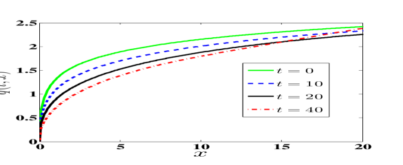
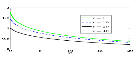
Figure 1: Production and exploration controls $(q,a)$ associated with the HJB equation (3.1) under constant price $p(t)=3$ and $\lambda(t)=(1-0.025t)^{+},0\leq t\leq T$. Left panel: production rate $q(t,x)$. Right panel: optimized exploration rate $a(t,x)$.

4.2 Numerical scheme for transport equation

We now assume given controls $q(t,x),a(t,x)$ and take up the evolution of the reserves distribution. To numerically solve the transport equations of $\eta(t,x)$ we use a fully explicit finite difference scheme which replaces derivatives with discretized increments of the respective functions over a grid. We use the same partition in the space domain $[0,X_{max}]$ using $\Delta x$ as in the previous section. To justify this bounded domain for the $x$-variable, recall the discussion about saturation level $x_{sat}$ at the end of Section 3.1 which motivates us to assume that $a(t,x)=0$ for $x$ large enough, and in turn implies that $\eta(t,x)=0$ for $x$ large enough (e.g. $x\geq\sup_{t}x_{sat}(t)+\delta$, with the additional assumption that the support of the initial distribution $\eta_{0}$ is also bounded). Thus, we apply the numerical boundary condition $\eta(t,X_{max})=0$ for all $t$. (Even if $a(t,x)>0$ for all $x$, we still expect that the right tail of $\eta$ should become negligible for $x$ large and so can be numerically truncated at $X_{Max}$.) Furthermore, we partition the time domain $[0,T]$ using a mesh $0=t_{0}<t_{1}<...<t_{N}=T$ with $t_{n}=n\Delta t$. To handle the boundary at $x=0$, the values $\eta(t,\cdot)$ and $q(t,\cdot)$ at $x=0+$ are numerically approximated by $\eta(t,x_{1})$ and $q(t,x_{1})$, respectively.

With the above setup, we approximate both derivatives in time and in space by forward difference quotients:

$$\frac{\partial}{\partial t}\eta(t_{n},x_{m})\approx\frac{\eta(t_{n+1},x_{m})-\eta(t_{n},x_{m})}{\Delta t},\quad\frac{\partial}{\partial x}\eta(t_{n},x_{m})\approx\frac{\eta(t_{n},x_{m+1})-\eta(t_{n},x_{m})}{\Delta x}.$$

By choosing $d=\lfloor\frac{\delta}{\Delta x}\rfloor$, so that $x_{m}-\delta\simeq x_{m-d}$ we approximate the integral term in (3.11a)–(3.11b) with a Riemann sum

$$-\int^{x_{m}}_{(x_{m}-\delta)_{+}}\lambda(t)a(t,x)\eta(t,dx)\approx\sum_{j=m-d+1\vee 1}^{m}\lambda(t_{n})a(t_{n},x_{j})\left(\eta(t_{n},x_{j-1})-\eta(t_{n},x_{j})\right),$$ (4.4)

where $\eta(t_{n},x_{j-1})-\eta(t_{n},x_{j})$ is the proportion of producers with reserves in the interval $[x_{j-1},x_{j}]$.

We start with given initial condition $\eta(t_{0},x_{m})=\eta_{0}(x_{m})$, $m=0,\ldots,M$, and solve forward in time using the right-edge boundary condition $\eta(t_{n},x_{M})=0$, $n=0,...,N$. We take $\eta(t_{n},x_{0})=1$ and interpret $\eta(t_{n},x_{1})\approx\eta(t_{n},0+)$ so that $\pi(t_{n})=\eta(t_{n},x_{0})-\eta(t_{n},x_{1})$. We then solve for $\eta(t_{n+1},\cdot)$ forward in space, splitting into cases according to $x_{m}\lessgtr\delta$. For $0<x_{m}<\delta$ (i.e. $m=1,2,\ldots$), which corresponds to (3.11a), we obtain the numerical value of $\eta(t_{n+1},x_{m})$ as

$$\eta(t_{n+1},x_{m}) =\eta(t_{n},x_{m})+\Delta tq(t_{n},x_{m})\frac{\eta(t_{n},x_{m+1})-\eta(t_{n},x_{m})}{\Delta x}$$

$$\quad-\Delta t\sum_{j=1}^{m}\lambda(t_{n})a(t_{n},x_{j})\left(\eta(t_{n},x_{j})-\eta(t_{n},x_{j-1})\right).$$ (4.5)

where the term for $j=1$ corresponds to $\lambda(t_{n})a(t_{n},0)\pi(t_{n})$ in (3.11a). For $x_{M}>x_{m}>\delta$, cf. -(3.11b), we obtain the numerical value of $\eta(t_{n+1},x_{m})$ by

$$\eta(t_{n+1},x_{m}) =\eta(t_{n},x_{m})-\Delta t\sum_{j=m-d+1}^{m}\lambda(t_{n})a(t_{n},x_{j})\left(\eta(t_{n},x_{j})-\eta(t_{n},x_{j-1})\right)$$

$$\qquad+q(t_{n},x_{m})\left(\eta(t_{n},x_{m+1})-\eta(t_{n},x_{m})\right)\frac{\Delta t}{\Delta x}.$$ (4.6)

Note that the above equations require only the values $a(t_{n},x_{m}),q(t_{n},x_{m})$ and there is no difficulty in combining a method-of-lines approach for the HJB portion of the MFG equations with the above fully discretized finite-difference scheme for the transport equation.

4.2.1 Illustrating the Evolution of Reserves Distribution

As an example suppose that the initial reserves distribution has a parabolic initial density $m_{0}(x)$

$$m_{0}(x)=\frac{6x(u-x)}{u^{3}}\quad\Leftrightarrow\quad\eta_{0}(x)=1-3(x/u)^{2}+2(x/u)^{3}\quad\text{for}\quad 0\leq x\leq u,$$

and $m_{0}(x)=0$ otherwise. In the example shown in Figure 2, we take $u=10$, cf. $m(0,x)$ on the left panel of the Figure. The evolution of boundary probability $\pi(t)=\mathbb{P}(X_{t}=0)$ and the density of reserves distribution $m(t,x)=-\frac{\partial}{\partial x}\eta(t,x)$ are shown in Figure 2. Numerically the density function is approximated by a difference quotient $m(t_{n},x_{m})\approx\frac{\eta(t_{n},x_{m})-\eta(t_{n},x_{m+1})}{\Delta x}$. Since discovery rate $\lambda(t)$ decreases in time, the reserves density $m(t,x)$ shifts towards zero as time evolves, as shown on the left panel of Figure 2. Similarly, the proportion $\pi(t)$ of producers with no remaining reserves increases in $t$ and zero global reserves are left shortly after discovery becomes impossible $\inf\{t:\pi(t)=1\}\simeq 41$, cf. right panel of Figure 2. We also note the discontinuity of $m(t,\cdot)$ at $x=\delta$ due to the discrete reserves jumps from $X_{t}=0$.

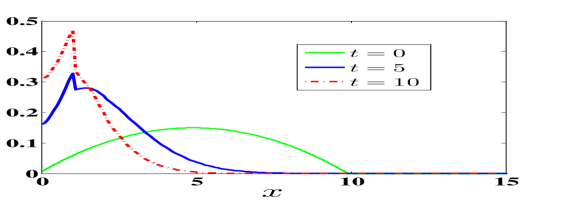
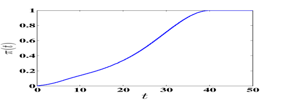
Figure 2: Evolution of reserves distribution under the production and exploration controls $(q,a)$ obtained in Section 4.1. The discovery rate is $\lambda(t)=(1-0.025t)^{+}$ and unit amount of a discovery is $\delta=1$. Left panel: Density of reserves distribution $m(t,x)=-\frac{\partial}{\partial x}\eta(t,x)$ for several $t$’s. Right: Proportion of producers with no reserves $\pi(t)=\mathbb{P}(X_{t}=0)$. After $t=41$ all reserves are exhausted.

4.3 Numerical scheme for the MFG system

We introduce an iterative scheme to solve the system of coupled HJB and transport equations. Our solution strategy consists of a loop over the following three steps. The loops are repeated over the iterations $k=0,1,\ldots$ until numerical convergence.

To initialize, we start with an initial price process $p^{(0)}(t)$ (greater than $\kappa_{1}$, to ensure strictly positive production rate). In Step 1, given the current $p^{(k)}(\cdot)$, the numerical scheme in Section 4.1 is implemented for the HJB equation, outputting the optimal production $q^{(k)}$ and exploration $a^{(k)}$ rates. Next in Step 2, these $q^{(k)}$ and $a^{(k)}$ are substituted into the transport equation to solve for $\eta^{(k)}$, following the scheme in Section 4.2. We then compute the total production $Q^{(k)}$ by using a Riemann sum to approximate the integral of $q^{(k)}(t,x)$ with respect to $\eta^{(k)}(t,\cdot)$. Finally, in Step 3 we update the price to $p^{(k+1)}$. Observe that if $p^{(k)}(t)$ is lower than equilibrium price $p^{\ast}(t)$ for all $t\in[0,T]$, the resulting $Q^{(k)}(t)$ will be lower than the equilibrium $Q(t)$. As a result, $D^{(-1)}(Q^{(k)}(t))$ will be higher than $p^{\ast}(t)$, and vice versa. Thus to speed up convergence, we take $p^{(k+1)}(t)$ in the next iteration to be the average of $p^{(k)}(t)$ and $D^{-1}(Q^{(k)}(t))$. Numerically we observe that this yields a monotone sequence of $p^{(k)}(t)$’s, improving convergence to the equilibrium $p^{\ast}(t)$.

Step 0. Start with an initial guess $p^{(0)}(t),t\in[0,T]$ of market price.

Step 1. For iteration $k=0,1,2,...$, and given $p^{(k)}(\cdot)$, solve the HJB equation (3.2) to obtain $v^{(k)}(t,x)$ and the corresponding $q^{(k)}(t,x)$ and $a^{(k)}(t,x)$ as in (3.13)-(3.14).

Step 2. With the above $q^{(k)}$ and $a^{(k)}$ solve the transport equation to obtain $\eta^{(k)}(t,x)$ satisfying (3.11).

Step 3. Update the market price via the new total quantity of production

$$p^{(k+1)}(t):=\frac{D^{-1}\left(Q^{(k)}(t)\right)+p^{(k)}(t)}{2}\ \quad\text{with}\quad Q^{(k)}(t)=\sum_{m=1}^{M-1}q^{(k)}(t,x_{m})[\eta^{(k)}(t,x_{m})-\eta^{(k)}(t,x_{m+1})].$$

Repeat Steps 1 — 3 until convergence in the sup-norm defined as $\left\|\cdot\right\|_{\infty}:=\sup_{[0,T]\times[0,X_{max}]}|\cdot|$. Iteration will stop when tolerance of error $TolError$ is satisfied

$$\left\|v^{(k+1)}-v^{(k)}\right\|_{\infty}<TolError,\quad\text{and}\quad\left\|\eta^{(k+1)}-\eta^{(k)}\right\|_{\infty}<TolError.$$ (4.7)

We continue with the running example where the discovery rate is $\lambda(t)=\left(1-0.025t\right)^{+}$, $\delta=1$ and initial price process is $p^{(0)}(t)=3\forall t$. Recall that the solutions obtained in Sections 4.1.1 and 4.2.1 can be viewed as the first iteration $k=0$ of the above scheme. Figure 3 illustrates the iterations over $k=0,1,\ldots$ with the resulting HJB value functions $v^{(k)}(t,x)$ at fixed time $t=10$. In each iteration $k$, if $v^{(k)}(t,x)$ is lower than the equilibrium value $v^{\ast}(t,x)$ for all $x\in[0,X_{max}]$ with some $t$ fixed, then in the next iteration $v^{(k+1)}(t,x)$ will move up towards the equilibrium level $v(t,x)$. This pointwise monotone convergence in $x$ is observed in Figure 3. Numerical convergence with a tolerance of $TolError=10^{-6}$ in (4.7) is achieved after $k=4$ iterations.

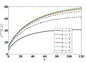
Figure 3: Convergence of the numerical scheme in Section 4.3. We start with initial guess $p^{(0)}(t)=3\forall t\in[0,T]$, and discovery rate $\lambda(t)=(1-0.025t)^{+}$. Game value function at $t=10$, $v^{(k)}(t,x)$, converges after $k\geq 4$ iterations.

Figure 4 shows the resulting evolution of total production $Q(t)$, total discovery rate $A(t)$, and total reserves level $R(t)$. Total reserves $R(t)$ decrease as production proceeds; in turn decreasing $R(t)$ lowers the total production rate $Q(t)$ and raises market price $p(t)$. Interestingly we observed a hump shape in $t\mapsto A(t)$: initially exploration efforts rise, then peak and gradually decline. This complex relationship is driven by the changing exploration success parameter $\lambda(t)$ (that discourages exploration as time progresses) and the reserves distribution $\eta(t,x)$ (which encourages exploration as reserves tend to get depleted on average).

To get some further insights, we compare these results with the non-exploration (NE) case that has zero discovery rate $\lambda(t)=0$. When $\lambda(t)=0$, no exploration effort will be made $a^{\ast}(t,x)\equiv 0$ as there is no hope to have any discovery. Consequently, producers simply gradually extract their initial reserves, eventually leading to total depletion, $R^{NE}(t)=0$ for $t>10.5$ in the Figure. This postponement of the reserves “Doomsday” is illustrated in the right-most panel of Figure 4 that plots the evolution of the proportion of exhausted producers’ $\pi(t)$. In comparison, for a model with exploration ultimate depletion only happens around $t=41$ (recall that $\lambda(t)=0$ after $t=40)$. In fact at $t=10$, less than 10% of producers have no reserves. As expected, because exploration increases global reserves, $R^{E}(t)\geq R^{NE}(t)$, the respective marginal value of reserves is lower and hence production is boosted, $Q^{E}(t)\geq Q^{NE}(t)\forall t$. Thus, exploration not only delays exhaustion but also unambiguously raises revenues.

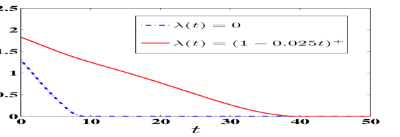
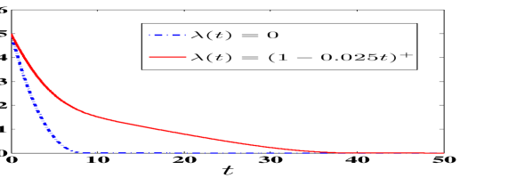
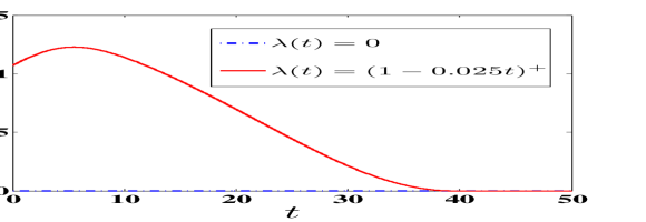
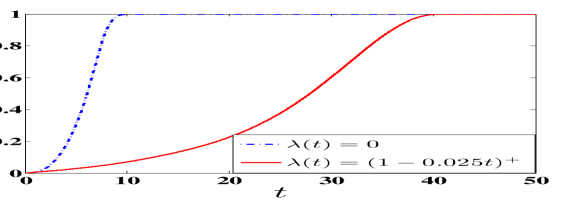
Figure 4: From left to right: evolution of total production $Q(t)$, total reserves $R(t)$, total discovery rate $A(t)$ and proportion $\pi(t)$ of producers with no reserves as a function of $t$. We show discovery rate $\lambda(t)=(1-0.025t)^{+}$, in comparison to no-exploration $\lambda(t)=0$.

5 Stationary mean field game Nash equilibrium

In Section 3 we studied a generic model with time-inhomogeneous discovery rate $\lambda(t)$, which would typically be taken to be decreasing in time. When there are still abundant resources underground, it is reasonable to assume that the discovery rate is time-homogeneous $\lambda(t)=\lambda$, for some $\lambda>0$. Thanks to exploration, the commodity used up for production can be compensated by new discoveries, and thus a stationary level of production and exploration can be obtained. In this section, we discuss such stationary MFG equilibria denoted by $(\tilde{q},\tilde{a},\tilde{\eta})$. Specifically, if the reserves has initial distribution $X_{0}\sim\tilde{\eta}$, and all the players apply the strategy $q_{t}=\tilde{q}(x;\tilde{\eta})$ and $a_{t}=\tilde{a}(x;\tilde{\eta})$, then the reserves process

$$dX_{t}=-\tilde{q}(X_{t})\mathds{1}_{\{X_{t}>0\}}dt+\delta d\tilde{N}_{t}$$ (5.1)

has the distribution $\tilde{\eta}(\cdot)$ for all $t>0$, that is, the reserves distribution is invariant in time. We define the stationary objective functional $\tilde{\mathcal{J}}$ of a player with current reserves level $x$ and conditionally on a reserves distribution $\tilde{\eta}(\cdot)$ as

$$\tilde{\mathcal{J}}(\tilde{q},\tilde{a};x,\tilde{\eta}):=\mathbb{E}\left\{\int_{0}^{\infty}\left[D^{-1}\left(\tilde{Q}(\tilde{\eta})\right)\tilde{q}(X_{t})-C_{q}(\tilde{q}(X_{t}))-C_{a}(\tilde{a}(X_{t}))\right]e^{-rt}dt\ \middle|\ X_{0}=x\right\},$$ (5.2)

where $\tilde{Q}(\tilde{\eta}):=-\int_{0}^{\infty}\tilde{q}(x)\tilde{\eta}(dx)$ is the stationary aggregate production.

Definition 5.1 (Stationary MFG MNE).

A stationary mean field game Nash equilibrium is a triple $\left(\tilde{q}^{\ast},\tilde{a}^{\ast},\tilde{\eta}\right)$ such that for $(X_{t})$ from (5.1) the distribution of reserves $\tilde{\eta}=\mathbb{P}(X_{t}\geq x)\forall t$ is unchanged under the strategies $(\tilde{q}^{\ast},\tilde{a}^{\ast})$, and

$$\tilde{v}(x)\equiv\tilde{\mathcal{J}}(\tilde{q}^{\ast},\tilde{a}^{\ast};\tilde{\eta})\geq\tilde{\mathcal{J}}(q,a;\tilde{\eta}),\quad\forall(q,a)\in\mathcal{A}.$$ (5.3)

The following Proposition 5.1 gives the system of stationary HJB and transport equations for $\tilde{v},\tilde{\eta}$ under a constant discovery rate $\lambda>0$. Intuitively, it is equivalent to the equations in the previous section after dropping the dependence on $t$. Consequently, we pass from PDE’s to ordinary differential equations in $x$.

Proposition 5.1 (Characterizing stationary MFG equilibrium).

The stationary value function $\tilde{v}$ and upper-CDF $\tilde{\eta}$ satisfy:

$$r\tilde{v}(x) =\left[-C_{a}(\tilde{a}^{\ast}(x))+\tilde{a}^{\ast}(x)\lambda\Delta_{x}\tilde{v}(x)\right]+\left[\tilde{p}\tilde{q}^{\ast}(x)-C_{q}(\tilde{q}^{\ast}(x))-\tilde{q}^{\ast}(x)\tilde{v}^{\prime}(x)\right],\quad x>0;$$ (5.4)

$$\begin{cases}0=\lambda\tilde{a}^{\ast}(0)(1-\tilde{\eta}(0+))-\int_{0+}^{x}\lambda\tilde{a}^{\ast}(z)\tilde{\eta}(dz)+\tilde{q}^{\ast}(x)\tilde{\eta}^{\prime}(x),\qquad 0<x\leq\delta,\\ 0=-\int_{x-\delta}^{x}\lambda\tilde{a}^{\ast}(z)\tilde{\eta}(dz)+\tilde{q}^{\ast}(x)\tilde{\eta}^{\prime}(x),\qquad\qquad\qquad x>\delta,\end{cases}$$ (5.5)

where the equilibrium stationary production and exploration rates ($\tilde{q}^{\ast}$, $\tilde{a}^{\ast}$) and price $\tilde{p}$ are

$$\tilde{q}^{\ast}(x)=\frac{1}{\beta_{1}}\left(L-\tilde{Q}-\kappa_{1}-\tilde{v}^{\prime}(x)\right)^{+},$$

$$\tilde{a}^{\ast}(x)=\frac{1}{\beta_{2}}\left(\lambda\Delta_{x}\tilde{v}(x)-\kappa_{2}\right)^{+},$$

$$\tilde{p}=D^{-1}\left(\tilde{Q}\right)=L+\int_{0}^{\infty}\tilde{q}^{\ast}(x)\tilde{\eta}(dx),$$ (5.6)

with $\tilde{Q}$ uniquely determined by the equation

$$\tilde{Q} =-\int_{0}^{\infty}\frac{1}{\beta_{1}}\left(L-\kappa_{1}-\tilde{v}^{\prime}(x)-\tilde{Q}\right)^{+}\tilde{\eta}(dx).$$ (5.7)

Similar to [25], the boundary condition for $\tilde{v}(0)$ is determined by

$$\tilde{v}(0)=\sup_{a\geq 0}\mathbb{E}\left[e^{-r\tau}\tilde{v}(\delta)-\int_{0}^{\tau}e^{-rt}C_{a}(a)dt\right]=\sup_{a\geq 0}\frac{a\lambda\tilde{v}(\delta)-C_{a}(a)}{r+a\lambda}.$$ (5.8)

Remark 5.1.

If the rate of new discoveries is zero, $\lambda=0$ then from the transport equation (5.5) we have $\tilde{\eta}^{\prime}(x)=0$ for all $x>0$, which implies that there is no producer with positive reserves level in the long run.

5.1 Solving for stationary MFG equilibria

For the stationary MFG developed in (5.4)-(5.5), the iterative scheme introduced in section 4.3 is not directly applicable. The challenge lies in solving the stationary transport equation (5.5). We see that the singularity at $x=0$ creates in effect a free boundary at $x=0$ that describes the balance between the density for $x>0$ and the point mass $\tilde{\pi}$ of exhausted producers. It is not clear how to directly handle this free boundary without ending with an intractable global system of coupled nonlinear equations.

To overcome this issue, we exploit the link between the time-dependent and time-stationary MFG models. Specifically, with a constant discovery rate $\lambda$ and large horizon $T$, the strategies $(v^{\ast},a^{\ast})$ have only weak dependence on $t$. Thus, we expect a convergence of the reserves process $X_{t}$ to an invariant distribution, since with a feedback, time-independent control it forms a recurrent Markov process on $\mathbb{R}_{+}$. This suggests to take $T$ large, solve the MFG on $[0,T]$ and then “extract” a $(\tilde{v},\tilde{a},\tilde{\eta})$ to approximate the true stationary solution.

A numerical illustration of a non-stationary MFG with constant discovery rate $\lambda(t)=\lambda\equiv 1$ is shown in Figure 5. The lower panels of Figure 5 show the evolution of total production $Q(t)$, total discovery $A(t)$, and total reserves level $R(t)$, which are defined by (3.15)-(3.18). We observe a boundary layer for small $t$ (roughly $t\in[0,12]$) arising from the non-equilibrium initial distribution $\eta_{0}(dx)$, and another boundary layer (roughly for $t\in[45,50]$) arising from the terminal condition $v(T,x)=0$. The latter causes $\lim_{t\to T}R(t)=0,\lim_{t\to T}A(t)=0$ observed in the plots. (Note that as the horizon is approached, total production rises in order to spend down all reserves and reach $R(T)=0$.) At the same time, for the intermediate $t$’s all the quantities are effectively time-independent and hence should be close to the stationary MFG equilibrium solution. In particular, due to the conservation of reserves, $R(t)\simeq 1.9$ for $t\in[15,45]$ we observe that $Q(t)\simeq A(t)$ on that time interval. Similarly, the respective reserves distribution $\eta(t,x)$ is almost independent of $t$, cf. the plot of $\pi(t)$ in Figure 5. Put another way, the actual value of the horizon $T$ is essentially irrelevant as it only determines where the end-of-the-world boundary layer appears (around $t=T-5$ in the plot) and has negligible effect on the solution prior to that.

A rigorous treatment of this phenomenon has been given in Cardaliaguet et al. [6] for a locally coupled MFG, and Cardaliaguet et al. [7] for a special case of a non-local coupling. According to [7], for each $t\in[0,T]$, the solution $(v(t,x),\eta(t,x))$ of a non-stationary MFG model converges in $L^{2}$-norm to the solution $(\tilde{v}(x),\tilde{\eta}(x))$ of stationary MFG model as $T\to\infty$. Furthermore, in their setting the difference between stationary and non-stationary mean field game equilibrium solutions, measured by $L^{2}$-norm, is minimized at $t=T/2$. Extending these proofs to the setting of Cournot MFGs with exploration is left for future research.

In light of these results, we can obtain an approximate solution of the stationary MFG MNE by solving the non-stationary equations (3.2) and (3.16) with constant discovery rate $\lambda(t)\equiv\lambda$, employing the same iterative scheme as in Section 4.3. Then the solution $(v(t,x),\eta(t,x))$ at $t=T/2$ is taken as approximate solution of the stationary mean field game model (5.4)-(5.5), i.e., $\tilde{v}(x)\approx v(T/2,x)$ and $\tilde{\eta}(x)\approx\eta(T/2,x)$ for all $x\in[0,X_{max}]$. A related approach was taken in Chan and Sircar [12] where the stationary MFG solution was obtained by solving non-stationary transport equation coupled with stationary HJB equation and taking the large time limit.

In the example shown in Figure 5 we had $T=50$, and so we use the intermediate solution $(v(t,x),\eta(t,x))\approx(\tilde{v}(x),\tilde{\eta}(x))$ at $t=T/2=25$ as an approximation to the corresponding time-stationary MFG. The upper left panel of Figure 5 shows the (approximate) stationary reserve density $\tilde{m}(x)\approx\frac{\partial}{\partial x}\eta(25,x)$. We observe that $\tilde{m}(x)$ increases in $x$ for $0<x\leq\delta$ where the rate of discovery is higher than the rate of production, and decreases for $x>\delta$. Similarly, we can extract the stationary total production $\tilde{Q}$, total discovery $\tilde{A}$, and total reserves level $\tilde{R}$ by looking at $Q(t),A(t),R(t)$ at $t=T/2=25$. (Due to conservation of mass $\tilde{A}=\tilde{Q}$.)

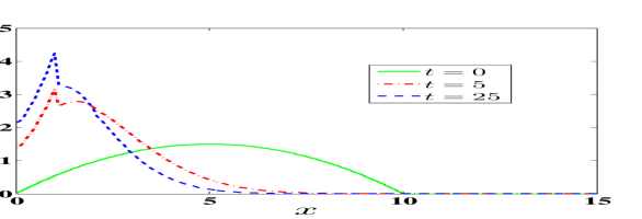
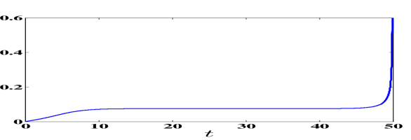
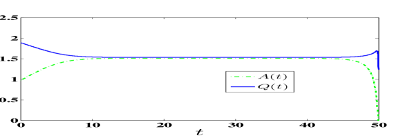
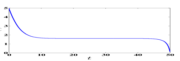
Figure 5: MFG solution with a constant $\lambda(t)\equiv\lambda=1$ and $T=50$ to illustrate the relationship between the time-dependent and stationary solutions. Upper left panel: Density $m(t,x)$ of reserves distribution. Upper right: Proportion $\pi(t)$ of producers without reserves. Lower left: Total exploration rate $A(t)$ and total production $Q(t)$. Lower right: Total reserves $R(t)$.

5.2 Comparative Statics for the Stationary MFG

It is instructive to study the effect of exploration on the equilibrium of the stationary mean field game. Figure 6 shows the effect of discovery rate $\lambda$ on the aggregate stationary quantities $\tilde{Q}$, $\tilde{A}$, and $\tilde{R}$, all of which have positive relation with $\lambda$. As discoveries take place faster with larger $\lambda$, the marginal value of each discovery decreases which yields an ambiguous effect to exploration effort $\tilde{a}^{\ast}$. In the top right panel of Figure 6) we observe that for low values of $\lambda$, $\lambda\to\tilde{a}^{\ast}(x;\lambda)$ increases, i.e. exploration is encouraged by higher likelihood of discovery. However, for high $\lambda$’s, $\lambda\to\tilde{a}^{\ast}(x;\lambda)$ is decreasing pointwise as the producer becomes “lazy” and does not see a need to work as hard, since new reserves are so easy to come by. In aggregate across $x$, we do observe a positive relation between $\lambda$ and total discovery rate $\tilde{A}$ (top left panel). Due to $\tilde{A}=\tilde{Q}$, this translates into higher aggregate production and lower prices.

Easier discoveries also raise the stationary level of reserves $\tilde{R}$, although the underlying impact on $\tilde{\eta}$ is non-monotone. This is illustrated in the bottom right panel of Figure 6 which plots the density $\tilde{m}(x)$ for several different $\lambda$’s and highlights multiple phenomena of interest. On the one hand, we observe that $\lambda\tilde{a}^{\ast}(0)$ monotonically increases in $\lambda$ which reduces the expected time until next discovery at $x=0$ and hence lowers the stationary proportion $\tilde{\pi}$. In the same vein, $\tilde{R}$ rises in $\lambda$ and shifts the whole $\tilde{m}$ to the right. On the other hand,, the spread, i.e. variance of $\tilde{m}$ starts falling as $\lambda$ keeps rising. Thus, for low $\lambda$, $\tilde{\eta}$ is more spread out and $\tilde{\pi}$ is higher; for high $\lambda$ $\tilde{\eta}$ is concentrated around the average $\tilde{R}$. Moreover, the support of $\tilde{m}$ has a hump shape in $\lambda$. Recall that due to exploration saturation, $\tilde{m}$ is supported on $[0,\tilde{x}_{sat}+\delta]$ where $\tilde{x}_{sat}$ is the saturation level. We find that $\tilde{x}_{sat}$ first rises and then falls in terms of $\lambda$. For example, when $\lambda=1$, we have $\tilde{x}_{s}at=64.8$ which can be compared to $\tilde{x}_{sat}(\lambda=0.2)=60.7$ and $\tilde{x}_{sat}(\lambda=10)=23.9$. In the latter situation when $\lambda$ is very big, there is no reason to hold many reserves (instead resources can be replenished almost instantaneously), so $\tilde{v}(x)$ approaches its horizontal asymptote quickly and hence exploration only takes place for small $x$. A further phenomenon is that when $\lambda$ is very small, e.g. $\lambda<0.05$ in Figure 6, exploration stops entirely ($\tilde{A}=0$ leading to $\tilde{R}=0$) in stationary equilibrium. This occurs because when $\kappa_{2}>0$ and $\lambda$ is small enough, the expected addition of value $\lambda\Delta_{x}\tilde{v}(x)$ is always smaller than the cost $\kappa_{2}$ and thus no exploration efforts will be made. Thus, when discoveries are “too difficult”, exploration will cease even if there are still potential new reserves remaining underground, $\lambda>0$.

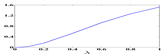
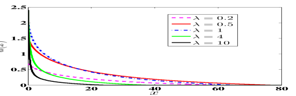
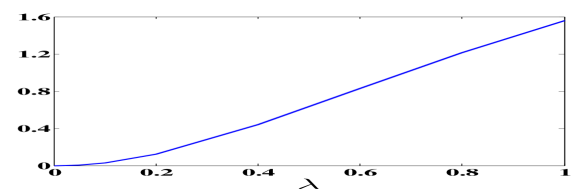
Figure 6: Stationary MFG solution as a function of discovery rate $\lambda$. Top Left panel: Stationary aggregate exploration/production $\tilde{A}=\tilde{Q}$. Top Right: Stationary exploration effort $\tilde{a}^{\ast}(x)$. Bottom Left: Stationary aggregate reserves $\tilde{R}=\int_{0}^{\infty}x\tilde{m}(dx)$; Bottom Right: Stationary distribution $\tilde{m}(x)$. Note that the total mass on $(0,\infty)$ is $1-\tilde{\pi}$ which depends on $\lambda$. As before, there is a discontinuity at $x=\delta=1$.

6 Fluid limit of exploration process

The stochasticity of the exploration process depends on two factors: the discovery rate $\lambda$ per unit exploration effort, and the size $\delta$ of each discovery. To study the effect of randomness of the exploration process on equilibrium production and reserves distribution we introduce an asymptotic parameter $\epsilon>0$ (cf. [21]), rescaling $\lambda_{\epsilon}:=\lambda/\epsilon$ and $\delta_{\epsilon}:=\delta\epsilon$. As $\epsilon\downarrow 0$, we have the discovery rate $\lambda_{\epsilon}\uparrow\infty$ and unit discovery amount $\delta_{\epsilon}\downarrow 0$, which means that the exploration process becomes more deterministic. In the sequel we use $\epsilon$ to index the respective MFG equilibria.

For the limiting case $\epsilon=0$ the exploration process is fully deterministic. This is known as the fluid limit since we fully average out the stochasticity in $(X_{t})$ without modifying its average (in the sense of expected value) behavior. Intuitively in the fluid limit, the difference term $\Delta_{x}v(t,x)=v(t,x+\delta)-v(t,x)$ becomes $\frac{\partial}{\partial x}v_{0}(t,x)$ and the integral becomes $\delta a_{0}^{*}(t,x)\frac{\partial}{\partial x}\eta_{0}(t,x)$, removing the non-local term. The resulting MFG equations are given by (6)–(6.2) below.

$$0=\frac{\partial}{\partial t}v_{0}(t,x)-rv_{0}(t,x)+\frac{1}{2\beta_{1}}\left[\left(p_{0}(t)-\kappa_{1}-\frac{\partial}{\partial x}v_{0}(t,x)\right)^{+}\right]^{2}$$

$$\quad+\frac{1}{2\beta_{2}}\left[\left(\lambda\delta\frac{\partial}{\partial x}v_{0}(t,x)-\kappa_{2}\right)^{+}\right]^{2};$$ (6.1)

$$\frac{\partial}{\partial t}\eta_{0}(t,x)=\left(-\lambda\delta a^{\ast}_{0}(t,x)+q^{\ast}_{0}(t,x)\right)\frac{\partial}{\partial x}\eta_{0}(t,x),\quad x>0,$$ (6.2)

where the optimal production rate $q^{\ast}_{0}$ and exploration rate $a^{\ast}_{0}$ are

$$q^{\ast}_{0}(t,x) =\arg\max_{q\geq 0}\left[p_{0}(t)q-C_{q}(q)-q\frac{\partial}{\partial x}v_{0}(t,x)\right]$$

$$=\frac{1}{\beta_{1}}\left(p_{0}(t)-\kappa_{1}-\frac{\partial}{\partial x}v_{0}(t,x)\right)^{+},$$ (6.3)

$$a^{\ast}_{0}(t,x) =\arg\max_{a\geq 0}\left[-C_{a}(a)+a\lambda\delta\frac{\partial}{\partial x}v_{0}(t,x)\right]=\frac{1}{\beta_{2}}\left(\lambda\delta\frac{\partial}{\partial x}v_{0}(t,x)-\kappa_{2}\right)^{+},$$ (6.4)

and $p_{0}(t)=L+\int_{0}^{\infty}q^{\ast}_{0}(t,x)\eta_{0}(t,dx)$. Note that there is no “boundary” at $x=0$ for $\eta_{0}$ because depletion is never explicitly encountered; it only imposes the constraint $a^{\ast}_{0}(t,0)\geq q^{\ast}_{0}(t,0)$. The boundary conditions $v_{0}(t,0)$ and $\frac{\partial}{\partial x}v_{0}(t,0)$ are given explicitly by the following Lemma proven in Appendix A.4.

Lemma 6.1.

The boundary conditions $v_{0}(t,0)$ and $\frac{\partial}{\partial x}v_{0}(t,0)$ satisfy

$$\frac{\partial}{\partial x}v_{0}(t,0)=\frac{\beta_{2}(p_{0}(t)-\kappa_{1})+\beta_{1}\lambda\delta\kappa_{2}}{\beta_{1}\lambda^{2}\delta^{2}+\beta_{2}};$$ (6.5)

$$v_{0}(t,0)=\int_{t}^{T}\left[\frac{\lambda\delta(p_{0}(s)-\kappa_{1})-\kappa_{2}}{\beta_{1}\lambda^{2}\delta^{2}+\beta_{2}}\right]^{2}(1+\lambda^{2}\delta^{2})\mathrm{e}^{-r(s-t)}ds.$$ (6.6)

By taking $T\to\infty$, we may then consider the stationary fluid limit MFG. Mathematically, this yields the simplest setup as it removes the non-local “delay” term associated with discrete exploration, as well as the time-dependence, leaving with a coupled system of two ODE’s. In fact, the following Proposition 6.1 implies that economically the stationary MFG in the fluid limit reduces to just a couple of algebraic relations.

Proposition 6.1 (Stationary mean field game equilibrium in fluid limit).

The stationary MFG MNE in fluid limit ($\epsilon=0$) is summarized as

1. The stationary reserves distribution is $\tilde{\pi}_{0}=1$, i.e. all producers hold no reserves, $\tilde{R}_{0}=0$.

2. The equilibrium total production $\tilde{Q}_{0}$ and market price in the fluid limit are given by

   $$\tilde{Q}_{0}=\tilde{q}^{\ast}_{0}(0)=\frac{[(L-\kappa_{1})\lambda\delta-\kappa_{2}]^{+}}{\beta_{2}+(1+\beta_{1})\lambda\delta},\quad\text{and}\qquad\tilde{p}_{0}=L-\tilde{Q}_{0};$$ (6.7)

3. The equilibrium exploration control is $\tilde{a}^{\ast}_{0}(x)=0$ $\forall x>0$ and

   $$\tilde{a}^{\ast}_{0}(0)=\frac{1}{\delta\lambda}\tilde{q}_{0}^{\ast}(0).$$ (6.8)

The proof of Proposition 6.1 is Appendix A.3. In the case of fluid limit $\epsilon=0$, discovery of new resources happens in a completely deterministic way, thus it is not necessary to hold reserves for production. Producers starting with positive reserves will not explore until reserves run out. Once reserves level reaches zero, equation (6.8) implies that a player without reserves will choose production and exploration strategies such that the production rate exactly equals the rate of reserves increment due to his exploration effort. This explains how zero reserves can be sustained in equilibrium. Overall, the above Proposition shows that the stationary equilibrium with deterministic exploration is trivial, i.e. only $x=0$ matters and the system of ODE’s effectively collapses to algebraic equations linking $\tilde{Q}_{0}$ and $\tilde{A}_{0}$ to model parameters. This shows that the stochastic model is strictly more complex than the deterministic one.

6.1 Numerical scheme and illustration

The iterative scheme in Section 4.3 is easily adapted to solve the fluid limit system (6)–(6.2). As in Section 4.1, we employ method of lines to numerically solve the HJB equation. The space derivative of $v_{0}(t,x)$ at each spatial grid point $x_{m}$ is approximated by a backward difference quotient $\frac{\partial}{\partial x}v_{0}(t,x_{m})\simeq\frac{v_{0}(t,x_{m})-v_{0}(t,x_{m-1})}{\Delta x}$ so that $\frac{\partial}{\partial t}v_{0}(t,x_{m})$ becomes a function of $v_{0}(t,x_{m})$ and $v_{0}(t,x_{m-1})$:

$$\frac{\partial}{\partial t}v_{0}(t,x_{m})=rv_{0}(t,x_{m})-\frac{1}{2\beta_{1}}\left[\left(p_{0}(t)-\kappa_{1}-\frac{v_{0}(t,x_{m})-v_{0}(t,x_{m-1})}{\Delta x}\right)^{+}\right]^{2}\\ -\frac{1}{2\beta_{2}}\left[\left(\lambda\delta\frac{v_{0}(t,x_{m})-v_{0}(t,x_{m-1})}{\Delta x}-\kappa_{2}\right)^{+}\right]^{2},\quad m=1,2,\ldots,M.$$ (6.9)

We use Matlab’s Runge-Kutta ODE solver ode45 to solve the system (6.9) of ordinary differential equations for $\{v(t,x_{m}):m=0,1,\ldots,M\}$ backward in time with boundary condition $v_{0}(t,x_{0})\equiv v_{0}(t,0)$ given by (6.6) and initial condition $v(T,x_{m})=0$ for all $m=0,1,...,M$.

We use forward in time and forward in space scheme to solve the transport equation (6.2). As in section 4.2, we also prescribe the boundary condition $\eta_{0}(t_{n},x_{M})=0$, $n=0,...,N$ at $x_{M}\equiv X_{max}$ which assumes that $X_{max}$ is larger than the saturation level. We directly set $\eta_{0}(t_{n},x_{0})=1$ and obtain the numerical values of $\eta_{0}(t_{n+1},x_{m})$ for $m=1,\ldots,M$ via

$$\eta_{0}(t_{n+1},x_{m}) =\eta_{0}(t_{n},x_{m})+\Delta t\left[-\lambda\delta a_{0}(t_{n},x_{m})+q_{0}(t_{n},x_{m})\right]\frac{\eta_{0}(t_{n},x_{m+1})-\eta_{0}(t_{n},x_{m})}{\Delta x}.$$

Figure 7 illustrates the resulting solution both in the time-dependent model described above (left panel) and its stationary version (middle and right panels) similar to Section 5. We observe two distinct features of interest. First, we find that uncertainty discourages exploration as the discounting effect lowers the NPV of putting in effort today for a delayed reward at discovery date $\tau$. As a result, more uncertainty decreases aggregate production $\tilde{Q}$ and raises prices. Second, uncertainty encourages “hoarding”, i.e. holding additional reserves as a buffer against running out due to depletion Consequently, $\tilde{R}_{\epsilon}$ increases in $\epsilon$ (right panel of Figure 7). At the same time, as $\epsilon\downarrow 0$ stationary reserves level $\tilde{R}_{\epsilon}\downarrow 0$. Indeed, in the limit $\epsilon=0$, production can be viewed as a perfect just-in-time supply chain: effort is expended to find an infinitesimal amount of new underground resources which are immediately extracted and sold for profit. Thus, exploration effort becomes equivalent to a secondary production cost, the cost of securing the commodity supply to exactly match the desired production rate, and the precautionary need for reserves vanishes. Thus we conclude that economically uncertainty regarding discoveries carries a cost.

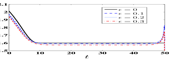
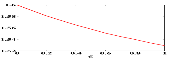
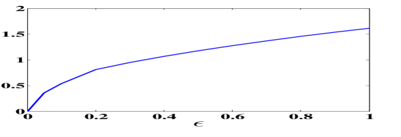
Figure 7: Equilibrium production and reserves level in the regime $\lambda_{\epsilon}=\lambda/\epsilon$ and $\delta_{\epsilon}=\delta\epsilon$ for different values of $\epsilon$. Left panel: Evolution of total production $Q_{\epsilon}(t)$ for several levels of $\epsilon$. Middle: Stationary production $\tilde{Q}_{\epsilon}$ against $\epsilon$. Right: Stationary reserves level $\tilde{R}_{\epsilon}$ against $\epsilon$. For $\epsilon=0$ we have $\tilde{Q}_{0}=\frac{5\cdot 1-0.2}{1+2\cdot 1}=1.6$ from (6.7) and $\tilde{R}_{0}=0$.

7 Conclusion

We investigate joint production and exploration of exhaustible commodities in a mean-field oligopoly. The ability to expend effort to find new resources creates several new phenomena that modify both the mathematical and economic structure of the market. First, exploration weakens the exhaustibility constraint and in particular permits existence of a stationary model where individual producer reserves evolve, but the market price and aggregate quantities are invariant over time. Second, exploration modifies the role of holding reserves —rather than determining future available means of production, reserves are partly used as a buffer to mitigate running out. As a result, if exploration is instantaneous and deterministic, no reserves are needed. This was explored in our analysis of the fluid limit model and connects to the early single-agent works from 1970s. Third, exploration control brings novel mathematical challenges to Cournot MFGs, in particular due to the non-local term (from discrete reserve events) in the transport equation and the non-smooth reserves distribution that involves a point mass at $x=0$ and a density on $(0,\infty)$. Fourth, the time-stationary Cournot MFG creates to a non-standard “free boundary” feature which required an approximation with a time-dependent version.

Among our insights is analysis about the ambiguous effects of exploration uncertainty and exploration frequency on the MFG equilibrium. This highlights the intricate interaction between stochasticity, reserves and the two types of controls, in addition to the game effects. A further important contribution is development of tailored numerical schemes to solve the various versions of the Cournot models which require different handling of the boundary conditions, of space- and time-dimensions and of the first-order-condition terms that determine the optimal controls.

In our illustrations, the role of time horizon $T$ was mainly secondary and only affected the discovery rate $\lambda(t)$. A more extensive calibration could be made to add additional $t$-dependency, which could be used as means to capture learning-by-doing, or to capture the intuition that discovery sizes might get smaller over time.

Another variant of the presented MFG approach would be to consider competition between a single major energy producer and a large population of minor energy producers, cf. [23, 10]. This would correspond for example to the dominant role played by the Organization of Petroleum Exporting Countries (OPEC) in the crude oil market, with OPEC controlling about 40% of the world’s oil production. Due to the resulting market power, the minor producers choose production strategies based on the production strategy of OPEC. The corresponding game model would involve a game value function for the major player, a game value function for a representative minor producer, and the reserves distribution of minor producers. The price is then determined by the aggregate production of the major plus all minor producers.

Another open problem is to establish the existence and uniqueness of the MFG MNE with stochastic discoveries, and the regularity of the associated value function. As discussed, the corresponding reserves distribution is non-smooth with a point mass at $x=0$, so only weak regularity is expected. Intuitively, better regularity might be possible if the discovery distribution is continuous (rather than a fixed amount $\delta$), although this could generate further challenges for the HJB equation, introducing a bonified integral term into (3.2). Such theoretical analysis could also help to rigorize the convergence of the proposed numerical scheme.

Appendix A Appendix

A.1 Proof of Proposition 3.1

Proof.

Given $T$, let $h(t,x)\in C^{\infty}_{c}((0,T)\times\mathds{R_{+}})$ be a test function that is compactly supported in $(0,T)\times\mathds{R_{+}}$. Using Itô’s formula for jump processes, and $h(T,X_{T})=h(0,X_{0})=0$ we have

$$0 =\mathbb{E}\left[h(T,X_{T})-h(0,X_{0})\right]$$

$$=\mathbb{E}\left[\int_{0}^{T}\frac{\partial}{\partial t}h(t,X_{t})-q(t,X_{t})\frac{\partial}{\partial y}h(t,X_{t})dt+\int_{0}^{T}[h(t,X_{t})-h(t-,X_{t-})]dN_{t}\right]$$

$$=-\int_{0}^{\infty}\int_{0}^{T}\frac{\partial}{\partial t}h(t,x)\frac{\partial}{\partial x}\eta(t,x)dtdx+\int_{0}^{\infty}\int_{0}^{T}q(t,x)\frac{\partial}{\partial x}h(t,x)\frac{\partial}{\partial x}\eta(t,x)dtdx$$

$$\quad-\int_{\delta}^{\infty}\int_{0}^{T}\left(h(t,x)-h(t,x-\delta)\right)\lambda(t)a(t,x-\delta)\frac{\partial}{\partial x}\eta(t,x-\delta)dtdx$$

$$\quad+\int_{0}^{T}h(t,\delta)\lambda(t)a(t,0)\pi(t)dt=:I1+I2+I3+I4.$$ (A.1)

By integration-by-parts and the fact that $h(t,x)$ has compact support in $(0,T)\times\mathds{R_{+}}$, the first term on the right hand side of the last equality of (A.1) equals to

$$I1 =\int_{0}^{\infty}\int_{0}^{T}\eta(t,x)\frac{\partial}{\partial t}\frac{\partial}{\partial x}h(t,x)dtdx=-\int_{0}^{\infty}\int_{0}^{T}\frac{\partial}{\partial x}h(t,x)\frac{\partial}{\partial t}\eta(t,x)dtdx.$$ (A.2)

By defining $F(t,x):=\int_{0}^{x}\lambda(t)a(t,z)\eta(t,dz)$, $x>0$, the third term on the right hand side of the last equality of (A.1) can be written as

$$I3 =-\int_{\delta}^{\infty}\int_{0}^{T}h(t,x)\frac{\partial}{\partial x}F(t,x-\delta)dtdx+\int_{0}^{\infty}\int_{0}^{T}h(t,x)\frac{\partial}{\partial x}F(t,x)dt\,dx$$

$$=\int_{\delta}^{\infty}\int_{0}^{T}F(t,x-\delta)\frac{\partial}{\partial x}h(t,x)dtdx-\int_{0}^{\infty}\int_{0}^{T}F(t,x)\frac{\partial}{\partial x}h(t,x)dt$$

$$=\int_{\delta}^{\infty}\int_{0}^{T}\left(F(t,x)-F(t,x-\delta)\right)\frac{\partial}{\partial x}h(t,x)dtdx-\int_{0}^{\delta}\int_{0}^{T}F(t,x)\frac{\partial}{\partial x}h(t,x)dt\,dx.$$ (A.3)

The fourth term on the right hand side of the last equality of (A.1) can be written as

$$I4 =\int_{0}^{T}\left(\int_{0}^{\delta}\frac{\partial}{\partial x}h(t,x)dx\right)\lambda(t)a(t,0)\pi(t)dt$$

$$=\int_{0}^{\delta}\int_{0}^{T}\lambda(t)a(t,0)\pi(t)\frac{\partial}{\partial x}h(t,x)dtdx.$$ (A.4)

By substituting (A.2)- (A.1) into equation (A.1), we obtain

$$0 =-\int_{0}^{\delta}\int_{0}^{T}\frac{\partial}{\partial x}h(t,x)\left[\frac{\partial}{\partial t}\eta(t,x)-q(t,x)\frac{\partial}{\partial x}\eta(t,x)+\int_{0+}^{x}\lambda a(t,z)\eta(t,dz)\right.$$

$$\quad\qquad\qquad\qquad\qquad+\lambda(t)a(t,0)\pi(t)\Bigr{]}dt\,dx$$

$$\quad-\int_{\delta}^{\infty}\int_{0}^{T}\frac{\partial}{\partial x}h(t,x)\left[\frac{\partial}{\partial t}\eta(t,x)-q(t,x)\frac{\partial}{\partial x}\eta(t,x)+\int_{x-\delta}^{x}\lambda a(t,z)\eta(t,dz)\right]dt\,dx,$$ (A.5)

which is true for any test function $h(t,x)\in C^{\infty}_{c}\left((0,T)\times\mathds{R_{+}}\right)$. According to the first term of the right hand side of (A.5), we have

$$0=\frac{\partial}{\partial t}\eta(t,x)-q(t,x)\frac{\partial}{\partial x}\eta(t,x)+\int_{0+}^{x}\lambda(t)a(t,z)\eta(t,dz)+\lambda(t)a(t,0)\pi(t),\quad 0<x<\delta.$$ (A.6)

According to the second term of the right hand side of (A.5), we have

$$0=\frac{\partial}{\partial t}\eta(t,x)-q(t,x)\frac{\partial}{\partial x}\eta(t,x)+\int_{x-\delta}^{x}\lambda(t)a(t,z)\eta(t,dz),\quad x>\delta.$$ (A.7)

The two equations (A.6) - (A.7) constitute the transport equation of reserves distribution given in Proposition 3.1.

∎

A.2 Proof of Lemma 3.2

Proof.

We integrate both sides of the transport equation (3.16) with respect to $x$ over $(0,\infty]$ to obtain

$$\int_{0+}^{\infty}\frac{\partial}{\partial t}\eta^{\ast}(t,x)dx =-\overbrace{\int_{0+}^{\delta}\left(\int_{0+}^{x}\lambda(t)a^{\ast}(t,z)\eta^{\ast}(t,dz)\right)\ dx}^{=:I1}-\overbrace{\int_{\delta}^{\infty}\left(\int_{x-\delta}^{x}\lambda(t)a^{\ast}(t,z)\eta^{\ast}(t,dz)\right)\ dx}^{=:I2}$$

$$\quad+\int_{0+}^{\infty}\left(q^{\ast}(t,x)\frac{\partial}{\partial x}\eta^{\ast}(t,x)\right)dx.$$ (A.8)

For the last term by definition of the Stieltjes integral, the integrator is equivalently $\frac{\partial}{\partial x}\eta^{\ast}(t,x)dx=\eta^{\ast}(t,dx)$. We apply integration by parts to the first two terms on the RHS of (A.8) to obtain

$$I1 =\left[x\int_{0+}^{x}\lambda(t)a^{\ast}(t,z)\eta^{\ast}(t,dz)\right]_{0+}^{\delta}-\int_{0+}^{\delta}x\frac{\partial}{\partial x}\left(\int_{0+}^{x}\lambda(t)a^{\ast}(t,z)\eta^{\ast}(t,dz)\right)dx$$

$$=\delta\int_{0+}^{\delta}\lambda(t)a^{\ast}(t,z)\eta^{\ast}(t,dz)-\int_{0+}^{\delta}x\lambda(t)a^{\ast}(t,x)\eta^{\ast}(t,dx),\qquad\text{and}$$ (A.9)

$$I2 =\left[x\int_{x-\delta}^{x}\lambda(t)a^{\ast}(t,z)\eta^{\ast}(t,dz)\right]_{x=\delta}^{x=\infty}-\int_{\delta}^{\infty}x\frac{\partial}{\partial x}\left(\int_{x-\delta}^{x}\lambda(t)a^{\ast}(t,z)\eta^{\ast}(t,dz)\right)dx$$

$$=-\delta\int_{0+}^{\delta}\lambda(t)a^{\ast}(t,z)\eta^{\ast}(t,dz)-\left[\int_{\delta}^{\infty}x\lambda(t)a^{\ast}(t,x)\eta^{\ast}(t,dx)-\int_{0+}^{\infty}(x+\delta)\lambda(t)a^{\ast}(t,x)\eta^{\ast}(t,dx)\right]$$

$$=-\delta\int_{0+}^{\delta}\lambda(t)a^{\ast}(t,z)\eta^{\ast}(t,dz)+\int_{0+}^{\delta}x\lambda(t)a^{\ast}(t,x)\eta^{\ast}(t,dx)+\delta\int_{0+}^{\infty}\lambda(t)a^{\ast}(t,x)\eta^{\ast}(t,dx).$$ (A.10)

The left hand side of (A.8) can be written as

$$\int_{0+}^{\infty}\frac{\partial}{\partial t}\eta^{\ast}(t,x)dx=\frac{d}{dt}\int_{0+}^{\infty}\eta^{\ast}(t,x)dx,$$ (A.11)

where the exchange of the partial differential operator and the integral is justified by the Leibniz integral rule under the condition that both $\eta^{\ast}(t,x)$ and $\frac{\partial}{\partial t}\eta^{\ast}(t,x)$ are continuous in the domain $(t,x)\in[0,\infty)\times(0,\infty)$. By substituting (A.9)–(A.11) into the equation (A.8), we have

$$\frac{d}{dt}\int_{0+}^{\infty}\eta^{\ast}(t,x)dx=-\delta\int_{0+}^{\infty}\lambda(t)a^{\ast}(t,x)\eta^{\ast}(t,dx)+\int_{0+}^{\infty}q^{\ast}(t,x)\eta^{\ast}(t,dx),$$

which gives (3.19). ∎

A.3 Proof of Proposition 6.1

We first present Lemmas A.1 and A.2 that summarize the partial differential equations associated with the fluid limit of our MFG model.

Lemma A.1.

The limiting game value function $v_{0}$ and reserves distribution function $(\tilde{\pi}_{0},\tilde{\eta}_{0})$ satisfy the following system

$$r\tilde{v}_{0}(x) =\left[\left(\tilde{p}_{0}-\tilde{v}^{\prime}_{0}(x)\right)\tilde{q}^{\ast}_{0}(x)-C_{q}(\tilde{q}^{\ast}_{0}(x))\right]+\left[-C_{a}(\tilde{a}^{\ast}_{0}(x))+\tilde{a}^{\ast}_{0}(x)\lambda\delta\tilde{v}^{\prime}_{0}(x)\right],\quad x\geq 0,$$ (A.12)

$$\begin{cases}0=-\lambda\delta\tilde{a}^{\ast}_{0}(0)\tilde{\pi}_{0}-\tilde{q}^{\ast}_{0}(0)\tilde{\eta}^{\prime}_{0}(0+),\\ 0=\left(-\lambda\delta\tilde{a}_{0}^{\ast}(x)+\tilde{q}_{0}^{\ast}(x)\right)\tilde{\eta}^{\prime}_{0}(x),\quad x>0,\end{cases}$$ (A.13)

where the optimal production rate $\tilde{q}^{\ast}_{0}$ and exploration rate $\tilde{a}^{\ast}_{0}$ are given by

$$\tilde{q}^{\ast}_{0}(x)=\frac{1}{\beta_{1}}\left(L-\tilde{Q}_{0}-\kappa_{1}-\tilde{v}_{0}^{\prime}(x)\right)^{+},$$

$$\tilde{a}^{\ast}_{0}(x)=\frac{1}{\beta_{2}}\left(\lambda\delta\tilde{v}^{\prime}_{0}(x)-\kappa_{2}\right)^{+},$$ (A.14)

and aggregate production $\tilde{Q}_{0}$ is uniquely determined by the equation

$$\tilde{Q}_{0} =-\int_{0}^{\infty}\frac{1}{\beta_{1}}\left(L-\kappa_{1}-\tilde{v}_{0}^{\prime}(x)-\tilde{Q}_{0}\right)^{+}\tilde{\eta}_{0}(dx),$$ (A.15)

and the equilibrium price is

$$\tilde{p}_{0}=L+\int_{0}^{\infty}\tilde{q}^{\ast}_{0}(z)\tilde{\eta}_{0}(dz).$$ (A.16)

Proof.

To obtain the HJB equation (A.12) of limiting game value function $\tilde{v}_{0}(x)$ and the associated optimal production controls (A.14), we let $\epsilon\to 0$, so that $\delta\epsilon\downarrow 0$ and $\lambda/\epsilon\uparrow\infty$ in the HJB equation (3.1) and the associated optimal production and exploration controls (3.3)-(3.4)

$$\tilde{a}^{\ast}_{0}(x)=\lim_{\epsilon\to 0}\tilde{a}^{\ast}_{\epsilon}(x) =\lim_{\epsilon\to 0}\frac{1}{\beta_{2}}\left[\lambda_{\epsilon}\left(\tilde{v}_{\epsilon}(x+\delta_{\epsilon})-\tilde{v}_{\epsilon}(x)\right)-\kappa_{2}\right]^{+}$$

$$=\lim_{\epsilon\to 0}\frac{1}{\beta_{2}}\left[\frac{\lambda}{\epsilon}\left(\tilde{v}_{\epsilon}(x+\delta\epsilon)-\tilde{v}_{\epsilon}(x)\right)-\kappa_{2}\right]^{+}$$

$$=\frac{1}{\beta_{2}}\left(\lambda\delta\tilde{v}_{0}^{\prime}(x)-\kappa_{2}\right)^{+},$$

$$\tilde{q}_{0}^{\ast}(x)=\lim_{\epsilon\to 0}\tilde{q}^{\ast}_{\epsilon}(x) =\lim_{\epsilon\to 0}\frac{1}{\beta_{1}}\left(L-\tilde{Q}_{\epsilon}-\kappa_{1}-\tilde{v}_{\epsilon}^{\prime}(x)\right)^{+}$$

$$=\frac{1}{\beta_{1}}\left(L-\tilde{Q}_{0}-\kappa_{1}-\tilde{v}_{0}^{\prime}(x)\right)^{+}.$$

Equations (A.13) and (A.15) follow similarly from (5.5) and (5.7). Note that as $\epsilon\downarrow 0$ the integral term $\int_{x-\delta_{\epsilon}}^{x}\lambda_{\epsilon}\tilde{a}_{\epsilon}(z)\tilde{\eta}_{\epsilon}(dz)$ in the third case $\delta_{\epsilon}<x$ of (3.16b) converges to

$$\lim_{\epsilon\to 0}\int_{x-\delta_{\epsilon}}^{x}\lambda_{\epsilon}\tilde{a}_{\epsilon}(z)\tilde{\eta}_{\epsilon}(dz)=\lim_{\epsilon\to 0}\int_{x-\delta\epsilon}^{x}\frac{\lambda}{\epsilon}\tilde{a}_{\epsilon}(z)\tilde{\eta}_{\epsilon}(dz)=\lambda\tilde{a}_{0}(x)\frac{\partial}{\partial x}\tilde{\eta}_{0}(x).$$

∎

Lemma A.2 (Fluid limit stationary boundary condition at $x=0$).

The equilibrium production and exploration rates in fluid limit on the boundary $x=0$ satisfy (6.8).

Proof.

On the boundary $x=0$ where there is no reserves, we must have $\delta\lambda\tilde{a}^{\ast}_{0}(0)\geq\tilde{q}^{\ast}_{0}(0)\geq 0$, i.e., the rate of reserves addition must be greater than or equal to production rate. If $a^{\ast}_{0}(0)=0$, it follows that $q^{\ast}_{0}(0)=\lambda\delta a^{\ast}_{0}(0)=0$. Now we consider the case that $a^{\ast}_{0}(0)>0$. Since $\tilde{q}^{\ast}_{0}(x)\geq 0$ is non-decreasing, and $\tilde{a}^{\ast}_{0}(x)$ decreases to $0$ as $x$ increases, we must have some point $x^{\ast}\geq 0$ such that $q_{0}^{\ast}(x^{\ast})=\lambda\delta a_{0}^{\ast}(x^{\ast})$. Note that once reserves process $X_{t}$ reaches the level $x^{\ast}$, it will remain unchanged since production rate $\tilde{q}_{0}^{\ast}(x^{\ast})$ is balanced by the rate of reserves increment $\lambda\delta\tilde{a}_{0}^{\ast}(x^{\ast})$ at $X_{t}=x^{\ast}$. We now prove that $x^{\ast}=0$. Towards a contradiction suppose that $x^{\ast}>0$. Then

$$\tilde{v}_{0}(x^{\ast}) =\int_{0}^{\infty}\left[\tilde{p}_{0}\tilde{q}^{\ast}_{0}(X^{x^{\ast}}_{t})-C_{q}(\tilde{q}^{\ast}_{0}(X^{x^{\ast}}_{t}))-C_{a}(\tilde{a}^{\ast}_{0}(X^{x^{\ast}}_{t}))\right]e^{-rt}dt$$

$$=\int_{0}^{\infty}\left[\tilde{p}_{0}\tilde{q}^{\ast}_{0}(x^{\ast})-C_{q}(\tilde{q}^{\ast}_{0}(x^{\ast}))-C_{a}(\tilde{a}^{\ast}_{0}(x^{\ast}))\right]e^{-rt}dt\leq\tilde{v}_{0}(0),$$

since starting at $x^{*}$, $X^{x^{*}}_{t}=x^{*}$ for all $t$, so that the resulting strategy $(\tilde{q}^{\ast}_{0}(x^{\ast}),\tilde{a}^{\ast}_{0}(x^{\ast}))$ is admissible for zero initial reserves and hence sub-optimal for the problem defining $\tilde{v}_{0}(0)$.

Next, let $\tau:=\inf\left\{t\geq 0:\int_{0}^{t}q^{\ast}_{0}(0)ds=x^{\ast}\right\}$.

$$\tilde{v}_{0}(0) =\int_{0}^{\tau}\left[\tilde{p}_{0}q^{\ast}_{0}(X^{0}_{t})-C_{q}(q^{\ast}_{0}(X^{0}_{t}))-C_{a}(\tilde{a}^{\ast}_{0}(X^{0}_{t}))\right]\mathrm{e}^{-rt}dt+\mathrm{e}^{-r\tau}\tilde{v}_{0}(X^{0}_{\tau})$$

$$<\int_{0}^{\tau}\left[\tilde{p}_{0}q^{\ast}_{0}(X^{0}_{t})-C_{q}(q^{\ast}_{0}(X^{0}_{t}))\right]\mathrm{e}^{-rt}dt+\mathrm{e}^{-r\tau}\tilde{v}_{0}(X^{0}_{\tau})\leq\tilde{v}_{0}(x^{\ast})$$ (A.17)

where the strict inequality $``>"$ is due to the assumption that $a^{\ast}_{0}(0)>0$ and the last inequality is due to the resulting strategy of starting at $x^{\ast}$, running reserves down to zero with zero exploration and then continuing with $\tilde{v}_{0}(X^{x^{\ast}}_{\tau})$ is admissible for the problem defining $\tilde{v}_{0}(x^{\ast})$ (treating $\tilde{p}_{0}$ fixed). The above two inequalities contradict each other; thus $x^{\ast}=0$, and $\tilde{q}_{0}^{\ast}(0)=\lambda\delta\tilde{a}_{0}^{\ast}(0)$. ∎

Using Lemmas A.1 and A.2, we prove Proposition 6.1.

Proof of proposition 6.1.

(i). Since $\tilde{q}^{\ast}_{0}(x)>0$ and $\tilde{a}^{\ast}_{0}(x)=0$ for $x>0$, we have $\tilde{\eta}^{\prime}_{0}(x)=0$ for $x>0$, according to the equation (A.13) in the interior. It follows that the reserves distribution degenerates to a point mass at 0, $\tilde{\pi}_{0}=1$. Substituting the latter fact into (A.15) we get

$$\tilde{Q}_{0} =\frac{1}{\beta_{1}}\left(L-\kappa_{1}-\tilde{v}_{0}^{\prime}(0)-\tilde{Q}_{0}\right)^{+},$$

which gives $\tilde{Q}_{0}=\frac{1}{1+\beta_{1}}\left(L-\kappa_{1}-\tilde{v}_{0}^{\prime}(0)\right)^{+}$ . According to (A.14) the equilibrium production rate at $x=0$ is

$$\tilde{q}^{\ast}_{0}(0) =\frac{1}{\beta_{1}}\left(L-\kappa_{1}-\tilde{v}_{0}^{\prime}(0)-\tilde{Q}_{0}\right)^{+}$$

$$=\frac{1}{1+\beta_{1}}\left(L-\kappa_{1}-\tilde{v}_{0}^{\prime}(0)\right)^{+}.$$ (A.18)

By substituting production rate (A.18) and exploration effort (A.14) with $x=0$ into the equation $\tilde{q}^{\ast}_{0}(0)=\lambda\delta\tilde{a}^{\ast}_{0}(0)$ and solving for $\tilde{v}_{0}^{\prime}(0)$, we obtain

$$\tilde{v}_{0}^{\prime}(0)=\frac{(L-\kappa_{1})\beta_{2}+\kappa_{1}(1+\beta_{1})}{\beta_{2}+(1+\beta_{1})\lambda\delta}.$$ (A.19)

Then by substituting the above $\tilde{v}_{0}^{\prime}(0)$ into (A.18) we have

$$\tilde{q}_{0}^{\ast}(0)=\frac{[(L-\kappa_{1})\lambda\delta-\kappa_{2}]^{+}}{\beta_{2}+(1+\beta_{1})\lambda\delta}.$$

Since $\tilde{\pi}_{0}=1$, we have $\tilde{Q}_{0}=-\int_{0}^{\infty}\tilde{q}^{\ast}_{0}(x)\tilde{\eta}_{0}(dx)=\tilde{q}^{\ast}_{0}(0)$ which yields (6.7). ∎

A.4 Proof of Lemma 6.1

Proof.

Similar to Lemma A.2, at $x=0$ we have

$$q_{0}^{\ast}(t,0)=\lambda\delta a_{0}^{\ast}(t,0).$$ (A.20)

By substituting (6.3)-(6.4) into (A.20), we obtain the boundary condition

$$\frac{\partial}{\partial x}v_{0}(t,0)=\frac{\beta_{2}(p_{0}(t)-\kappa_{1})+\beta_{1}\lambda\delta\kappa_{2}}{\beta_{1}\lambda^{2}\delta^{2}+\beta_{2}}.$$

Substituting (6.5) into (6.3)-(6.4), we obtain $a^{\ast}_{0}(t,0)$ and $q^{\ast}_{0}(t,0)$ in explicit form

$$a^{\ast}_{0}(t,0)=\frac{\lambda\delta(p_{0}(t)-\kappa_{1})-\kappa_{2}}{\beta_{1}\lambda^{2}\delta^{2}+\beta_{2}},$$ (A.21)

$$q^{\ast}_{0}(t,0)=\frac{\lambda^{2}\delta^{2}(p_{0}(t)-\kappa_{1})-\lambda\delta\kappa_{2}}{\beta_{1}\lambda^{2}\delta^{2}+\beta_{2}}.$$ (A.22)

By substituting (6.5), (A.21), and (A.22) into the HJB equation (6), we obtain the following linear first-order differential equation for $v_{0}(\cdot,0)$:

$$0 =\frac{\partial}{\partial t}v_{0}(t,0)-rv_{0}(t,0)+\frac{1}{2}\left[(a^{\ast}_{0}(t,0))^{2}+(q^{\ast}_{0}(t,0))^{2}\right],\qquad 0<x,\ 0\leq t<T,$$

which admits an explicit solution

$$v_{0}(t,0) =v_{0}(T,0)\mathrm{e}^{-r(T-t)}+\int_{t}^{T}\frac{1}{2}\left[(a^{\ast}_{0}(s,0))^{2}+(q^{\ast}_{0}(s,0))^{2}\right]\mathrm{e}^{-r(s-t)}ds$$

that matches (6.6) since $v_{0}(T,0)=0$. ∎

References

• [1] Y. Achdou, F. Camilli, and I. Capuzzo-Dolcetta, Mean field games: convergence of a finite difference method, SIAM Journal on Numerical Analysis, 51 (2013), pp. 2585–2612.
• [2] Y. Achdou and A. Porretta, Convergence of a finite difference scheme to weak solutions of the system of partial differential equations arising in mean field games, SIAM Journal on Numerical Analysis, 54 (2016), pp. 161–186.
• [3] K. J. Arrow and S. Chang, Optimal pricing, use, and exploration of uncertain resource stocks, Journal of Environmental Economics and Management, 9 (1) (1982), pp. 1–10.
• [4] A. Bensoussan, J. Frehse, and P. Yam, Mean Field Games and Mean Field Type Control Theory, Springer, 2013.
• [5] P. Cardaliaguet and P. J. Graber, Mean field games systems of first order, ESAIM: Control, Optimisation and Calculus of Variations, 21 (2015), pp. 690–722.
• [6] P. Cardaliaguet, J.-M. Lasry, P.-L. Lions, and A. Porretta, Long term average of mean field games, Networks & Heterogeneous Media, 7 (2012), pp. 279–301.
• [7] P. Cardaliaguet, J.-M. Lasry, P.-L. Lions, and A. Porretta, Long time average of mean field games with a nonlocal coupling, SIAM Journal on Control and Optimization, 51 (2013), pp. 3558–3591.
• [8] E. Carlini and F. J. Silva, A fully discrete semi-Lagrangian scheme for a first order mean field game problem, SIAM Journal on Numerical Analysis, 52 (2014), pp. 45–67.
• [9] R. Carmona, Lectures on BSDEs, Stochastic Control, and Stochastic Differential Games with Financial Applications, SIAM, 2016.
• [10] R. Carmona, X. Zhu, et al., A probabilistic approach to mean field games with major and minor players, The Annals of Applied Probability, 26 (2016), pp. 1535–1580.
• [11] P. Chan and R. Sircar, Bertrand & Cournot mean field games, Applied Mathematics & Optimization, 71 (2015), pp. 533–569.
• [12] P. Chan and R. Sircar, Fracking, renewables, and mean field games, SIAM Review, 59 (2017), pp. 588–615.
• [13] A. Dasarathy and R. Sircar, Variable costs in dynamic Cournot energy markets, in Energy, Commodities and Environmental Finance, M. L. R. Aid and R. Sircar, eds., Fields Insititute Communications, Fields Institute, 2014.
• [14] P. S. Dasgupta and G. M. Heal, Economic theory and exhaustible resources, Cambridge University Press, 1979.
• [15] S. D. Deshmukh and S. R. Pliska, Optimal consumption and exploration of nonrenewable resources under uncertainty, Econometrica, 48 (1980), pp. 177–200.
• [16] P. J. Graber, Linear quadratic mean field type control and mean field games with common noise, with application to production of an exhaustible resource, Applied Mathematics & Optimization, 74 (2016), pp. 459–486.
• [17] P. J. Graber and A. Bensoussan, Existence and uniqueness of solutions for Bertrand and Cournot mean field games, Applied Mathematics & Optimization, (2015), pp. 1–25.
• [18] P. J. Graber and C. Mouzouni, Variational mean field games for market competition, tech. report, arXiv preprint arXiv:1707.07853, 2017.
• [19] O. Guéant, Mean field games and applications to economics, PhD thesis, Université Paris-Dauphine, 2009.
• [20] O. Guéant, J.-M. Lasry, and P.-L. Lions, Mean field games and applications, in Paris-Princeton Lectures on Mathematical Finance, Springer, 2011, pp. 205–266.
• [21] P. S. Hagan, D. E. Woodward, R. E. Caflisch, and J. B. Keller, Optimal pricing, use and exploration of uncertain natural resources, Applied Mathematical Finance, 1 (1994), pp. 87–108.
• [22] C. Harris, S. Howison, and R. Sircar, Games with exhaustible resources, SIAM Journal of Applied Mathematics, 70 (2010), pp. 2556–2581.
• [23] M. Huang, Large-population LQG games involving a major player: the Nash certainty equivalence principle, SIAM Journal on Control and Optimization, 48 (2010), pp. 3318–3353.
• [24] A. Ledvina and R. Sircar, Oligopoly games under asymmetric costs and an application to energy production, Mathematics and Financial Economics, 6 (2012), pp. 261–293.
• [25] M. Ludkovski and R. Sircar, Exploration and exhaustibility in dynamic Cournot games, European Journal of Applied Mathematics, 23 (2011), pp. 343–372.
• [26] M. Ludkovski and X. Yang, Dynamic Cournot models for production of exhaustible commodities under stochastic demand, in Energy, Commodities and Environmental Finance, M. L. R. Aid and R. Sircar, eds., Fields Insititute Communications, Fields Institute, 2014.
• [27] R. Pindyck, The optimal exploration and production of nonrenewable resources, Journal of Political Economy, 86 (1978), pp. 841–862.
• [28]  , Uncertainty and exhaustible resource markets, Journal of Political Economy, 88 (6) (1980), pp. 1203–1225.