Kumaraswamy autoregressive moving average models for double bounded environmental data

Abstract

In this paper we introduce the Kumaraswamy autoregressive moving average models (KARMA), which is a dynamic class of models for time series taking values in the double bounded interval $(a,b)$ following the Kumaraswamy distribution. The Kumaraswamy family of distribution is widely applied in many areas, especially hydrology and related fields. Classical examples are time series representing rates and proportions observed over time. In the proposed KARMA model, the median is modeled by a dynamic structure containing autoregressive and moving average terms, time-varying regressors, unknown parameters and a link function. We introduce the new class of models and discuss conditional maximum likelihood estimation, hypothesis testing inference, diagnostic analysis and forecasting. In particular, we provide closed-form expressions for the conditional score vector and conditional Fisher information matrix. An application to environmental real data is presented and discussed.

1 Introduction

The Kumaraswamy family of distribution was introduced in Kumaraswamy (1980) for modeling double bounded random processes with hydrological applications. It is very flexible being able to approximate several types of distributions and its density can present many shapes, such as unimodal, uniantimodal, increasing, decreasing or constant. The Kumaraswamy distribution has been applied to a wide variety of problems, especially in hydrology (Nadarajah, 2008).

We say that a continuous random variable $\tilde{Y}$ follows a Kumaraswamy distribution with shape parameters $\varphi>0$ and $\delta>0$ and support in $(a,b)$ if its probability density function is given by (Mitnik, 2013):

$$f(\tilde{y};\varphi,\delta)=\frac{\varphi\delta}{b-a}\left(\frac{\tilde{y}-a}{b-a}\right)^{\varphi-1}\left[1-\left(\frac{\tilde{y}-a}{b-a}\right)^{\varphi}\right]^{\delta-1},$$

for $a<\tilde{y}<b$. In this case we denote $\tilde{Y}\sim K(\delta,\varphi,a,b)$. The cumulative distribution and quantile functions are, respectively, given by:

$$F(\tilde{y})=1-\left[1-\left(\frac{\tilde{y}-a}{b-a}\right)^{\varphi}\right]^{\delta}\quad\mbox{ and }\quad F^{-1}(u)=a+(b-a)\left[1-(1-u)^{\frac{1}{\delta}}\right]^{\frac{1}{\varphi}},\quad 0<u<1.$$

The mean and variance of $\tilde{Y}$ are given by

$$\mathds{E}(\tilde{Y})=a+(b-a)\delta\texttt{B}\left(1+\frac{1}{\varphi},\delta\right)$$ (1)

and

$$\operatorname{Var}(\tilde{Y})=(b-a)^{2}\left\{\delta\texttt{B}\left(1+\frac{2}{\varphi},\delta\right)-\left[\delta\texttt{B}\left(1+\frac{1}{\varphi},\delta\right)\right]^{2}\right\},$$ (2)

where $\texttt{B}(\cdot,\cdot)$ is the Beta function (Gupta and Nadarajah, 2004). Some properties of the Kumaraswamy distribution can be found in Jones (2009), Gupta and Nadarajah (2004), and Mitnik (2013). It is usually applied as a more tractable alternative to the beta distribution (Jones, 2009; Nadarajah, 2008; Mitnik and Baek, 2013).

The beta distribution has been widely applied to model double bounded variates. The beta regression model (Ferrari and Cribari-Neto, 2004), for example, which resembles the generalized linear models (GLM) (McCullagh and Nelder, 1989), has been generalized, improved and applied in several works (Cribari-Neto and Zeileis, 2010; Simas et al., 2010; Ospina and Ferrari, 2012; Bayer and Cribari-Neto, 2013; Souza and Cribari-Neto, 2015). Beta related models for time series have also received attention in the literature. See for instance Rocha and Cribari-Neto (2009), da Silva et al. (2011), Guolo and Varin (2014), Palm and Bayer (2017) and references therein.

The flexibility of the beta distribution encourages its empirical use in a wide range of applications (Lemonte et al., 2013; Jones, 2009; Nadarajah, 2008). However, the beta distribution does not satisfactorily fit hydrological process such as daily rainfall, daily stream flow, etc (Kumaraswamy, 1976, 1980; Lemonte et al., 2013). On the other hand, in hydrology and related areas, the Kumaraswamy distribution is deemed as a better alternative to the beta distribution (Nadarajah, 2008; Lemonte et al., 2013), so that several works applying the Kumaraswamy distribution can be found (Nadarajah, 2008). This is also true in the Engineering literature, as, for instance, in Sundar and Subbiah (1989), Fletcher and Ponnambalam (1996), Seifi et al. (2000), Ponnambalam et al. (2001), Ganji et al. (2006), and Koutsoyiannis and Xanthopoulos (1989).

Despite its importance and wide range of applications in hydrology, the Kumaraswamy distribution is still a stranger for statisticians. In fact, the lack of tractable expressions for the mean and variance, given by (1) and (2), respectively, has hindered its utilization for modeling purposes (Lemonte et al., 2013; Mitnik and Baek, 2013). An alternative to circumvent this problem is to consider a median-based re-parameterization aiming to facilitate its use in regression-based models (Mitnik and Baek, 2013). For the Kumaraswamy distribution, the median has the following simple expression:

$$md(\tilde{Y})=\tilde{\mu}=a+(b-a)\left(1-0.5^{\frac{1}{\delta}}\right)^{\frac{1}{\varphi}},$$

where $\left(1-0.5^{\frac{1}{\delta}}\right)^{\frac{1}{\varphi}}=\mu$ is the median of the rescaled variable $Y=\frac{\tilde{Y}-a}{b-a}\in(0,1)$.

Most time series appearing in natural sciences, including hydrology, climatology and environmental applications consist of observations that are serially dependent overtime (Salas et al., 1997; Machiwal and Jha, 2012; Lohani et al., 2012; Valipour et al., 2013). Most conventional time series models are based on Gaussianity assumptions (Chuang and Yu, 2007). One classical example is the class of autoregressive integrated moving average models (ARIMA) (Box et al., 2008; Brockwell and Davis, 1991). However, it has been recognized that the Gaussian assumption is too restrictive for many applications (Tiku et al., 2000), specially in hydrology. Indeed, as previously discussed, several double bounded hydrologic data can be accurately modeled by the Kumaraswamy distribution. Despite of this, to the best of our knowledge, a specific time series model to serially dependent Kumaraswamy variables has never been considered in the literature. Thus, in this work our goal is to introduce and study a dynamic time series model for Kumaraswamy distributed random variables. In order to define the proposed model, we shall follow similar construction as the generalized autoregressive and moving average model (GARMA) (Benjamin et al., 2003) and the beta autoregressive and moving average model ($\beta$ARMA) (Rocha and Cribari-Neto, 2009), but we shall employ a parametrization for the Kumaraswamy distribution in terms of its median.

The paper is organized as follows. In Section 2 we introduce the proposed model. In Section 3 we present a complete conditional maximum likelihood theory for KARMA models, including closed forms for the conditional score vector and Fisher information matrix and the related asymptotic theory. The construction of confidence intervals and hypothesis testing is also discussed. On Section 4 we present several topics regarding model diagnostics and forecasting. In Section 5 we present a Monte Carlo simulation study to assess the finite sample performance of the conditional maximum likelihood approach developed. An application of KARMA models to relative humidity data is presented in Section 6. Section 7 closes the article. For ease of presentation, some technical results are deferred to the Appendix.

2 The proposed model

In order to define the proposed model, we shall introduce an autoregressive moving average (ARMA) time series structure to accommodate the presence of serial correlation in the conditional median of the Kumaraswamy distribution. For this reason, we shall call the proposed model as KARMA model. We shall employ a similar parameterization as in Mitnik and Baek (2013), where $\mu=(1-0.5^{\frac{1}{\delta}})^{\frac{1}{\varphi}}$, i.e., $\delta=\frac{\log(0.5)}{\log(1-\mu^{\varphi})}$. We shall write $\tilde{Y}\sim K(\tilde{\mu},\varphi,a,b)$. Furthermore, $Y=(\tilde{Y}-a)/(b-a)$ follows a $K(\mu,\varphi,0,1)$, where $\mu$ is given by $\mu=(\tilde{\mu}-a)/(b-a)$. For simplicity, in this case we shall write $Y\sim K(\mu,\varphi)$. From this point on we shall only consider the Kumaraswamy distribution parameterized in terms of its median (see Figure 1).

Now let $\{\tilde{Y}_{t}\}_{t\in\mathds{Z}}$ be a stochastic process for which, $\tilde{Y}_{t}\in(a,b)$ with probability 1, for all $t\in\mathds{Z}$ and fixed $a,b\in\mathds{R}$ with $a<b$ and let $\mathscr{F}_{t}=\sigma\{\tilde{Y}_{t},\tilde{Y}_{t-1},\dots\}$ denote the sigma-field generated by the information observed up to time $t\in\mathds{Z}$. Assume that, conditionally to the previous information set $\mathscr{F}_{t-1}$, $\tilde{Y}_{t}$ is distributed according to $K(\tilde{\mu}_{t},\varphi,a,b)$ and let $Y_{t}=(\tilde{Y}_{t}-a)/(b-a)$, $t\in\mathds{Z}$. It follows that $Y_{t}|\mathscr{F}_{t-1}\sim K(\mu_{t},\varphi)$. The conditional density of $\tilde{Y}_{t}$ given $\mathscr{F}_{t-1}$ is

$$f_{\mu_{t}}(\tilde{y}_{t}\mid\mathscr{F}_{t-1})=\left(\frac{1}{b-a}\right)\frac{\varphi\log(0.5)}{\log(1-{\mu}_{t}^{\varphi})}{y}_{t}^{\varphi-1}(1-{y}_{t}^{\varphi})^{\frac{\log(0.5)}{\log(1-{\mu}_{t}^{\varphi})}-1},\quad 0<\mu_{t}<1,\;\;\varphi>0,$$ (3)

for $0<y_{t}<1$, where ${y}_{t}=\frac{\tilde{y}_{t}-a}{b-a}$, ${\mu}_{t}=\frac{\tilde{\mu}_{t}-a}{b-a}$. This particular form of the density is very appealing since it allows modeling without any transformation, as it is commonly done in literature (see, for instance, Rocha and Cribari-Neto, 2009), but dealing with the simpler distribution of $Y_{t}$.

(a) $\mu=0.25$ and values of $\varphi$ indicated in the graph

(b) $\varphi=2$ and values of $\mu$ indicated in the graph

Figure 1: Kumaraswamy density functions for several values of parameters $\mu$ and $\varphi$ (with $a=0$ and $b=1$).

The cumulative distribution and quantile functions, are given respectively by:

$$F_{\mu_{t}}(\tilde{y}_{t}\mid\mathscr{F}_{t-1}) =1-(1-{y}_{t}^{\varphi})^{\frac{\log(0.5)}{\log(1-{\mu}_{t}^{\varphi})}},$$

$$F_{\mu_{t}}^{-1}(u\mid\mathscr{F}_{t-1}) =a+(b-a)\left[1-(1-u)^{\frac{\log(1-{\mu}_{t}^{\varphi})}{\log(0.5)}}\right]^{\frac{1}{\varphi}}.$$

The conditional mean and variance of $\tilde{Y}_{t}$, in terms of $\mu_{t}$ and $\varphi$, are given respectively by:

$$\mathds{E}(\tilde{Y}_{t}\mid\mathscr{F}_{t-1}) =a+(b-a)\frac{\log(0.5)}{\log(1-{\mu}_{t}^{\varphi})}\texttt{B}\left(1+\frac{1}{\varphi},\frac{\log(0.5)}{\log(1-{\mu}_{t}^{\varphi})}\right),$$

$$\operatorname{Var}(\tilde{Y}_{t}\mid\mathscr{F}_{t-1}) =\frac{1}{b-a}\bigg{\{}\frac{\log(0.5)}{\log(1-{\mu}_{t}^{\varphi})}\texttt{B}\left(1+\frac{2}{\varphi},\frac{\log(0.5)}{\log(1-{\mu}_{t}^{\varphi})}\right)-\left[\frac{\log(0.5)}{\log(1-{\mu}_{t}^{\varphi})}\texttt{B}\left(1+\frac{1}{\varphi},\frac{\log(0.5)}{\log(1-{\mu}_{t}^{\varphi})}\right)\right]^{2}\bigg{\}}.$$ (4)

Let $g:\mathds{R}\rightarrow(0,1)$ be a continuously twice differentiable monotone link function for which the inverse $g^{-1}:(0,1)\rightarrow\mathds{R}$ exists and is twice continuously differentiable as well. We propose the following specification for the conditional median $\mu_{t}$:

$$\eta_{t}=g(\mu_{t})=\alpha+x_{t}^{\top}\beta+\sum_{i=1}^{p}\phi_{i}\big{[}g(y_{t-i})-x^{\top}_{t-i}\beta\big{]}+\sum_{j=1}^{q}\theta_{j}r_{t-j},$$ (5)

where $\eta_{t}$ is the linear predictor, $x_{t}$ is the $r$-dimensional vector containing the covariates at time $t$, $\beta=(\beta_{1},\dots,\beta_{r})^{\top}$ is the $r$-dimensional vector of parameters related to the covariates, while $\phi=(\phi_{1},\dots,\phi_{p})^{\top}$ and $\theta=(\theta_{1},\dots,\theta_{q})^{\top}$ are the AR and MA coefficients, respectively. As usual, we shall assume that the AR and MA characteristic polynomials do not have common roots and the AR coefficients are such that the related characteristic polynomial does not have unit roots. Invertibility and causality conditions for the ARMA component are not needed and, thus, not required. For more details on ARMA modeling, we refer the reader to Brockwell and Davis (1991). Observe that, since $\mu_{t}\in(0,1)$, all the traditional link functions such as logit, probit, loglog, etc, can be applied to the model. Results related to $\tilde{\mu}_{t}$ and $\tilde{y}_{t}$, such as predicted values and confidence intervals, can be easily obtained through $\tilde{\mu}_{t}=\mu_{t}(b-a)+a$ and $\tilde{y}_{t}=y_{t}(b-a)+a$.

The proposed KARMA$(p,q)$ model is given by specification (3) and (5). We observe that the dynamic part of the model (5) is the same as in Rocha and Cribari-Neto (2009). However, the random component of the model (3) is completely different and it is parametrized in terms of the median. Regression methods based on the median are known to be robust against atypical observations in the response (John, 2015; Lemonte and Bazán, 2016). It is also known that, compared to mean based models, median based ones present a better performance when the population distribution is asymmetric (Lemonte and Bazán, 2016). Since the specification (5) is based on the median, the proposed KARMA model inherits these attractive properties.

3 Conditional likelihood inference

Parameter estimation can be carried out by conditional maximum likelihood. The boundary parameters $a$ and $b$ are assumed to be either known (as it is often the case for rates and proportions) or previously consistently estimated. Let $\tilde{y}_{1},\dots,\tilde{y}_{n}$ be a sample from a KARMA$(p,q)$ model under specification (3) and (5), where $x_{t}$ denote the $r$-dimensional vector of covariates for $y_{t}$, assumed to be non-stochastic and let $\gamma=(\alpha,\beta^{\top},\phi^{\top},\theta^{\top},\varphi)^{\top}$ be the $(p+q+r+2)$-dimensional parameter vector. The conditional maximum likelihood estimators (CMLE) are obtained upon maximizing the logarithm of the conditional likelihood function. We observe that the log-likelihood function for $\gamma$, conditionally on $\mathscr{F}_{t-1}$, is null for the first $m=\max(p,q)$ values of $t$, and hence we have

$$\ell=\ell(\gamma;\tilde{y}_{t})=\sum\limits_{t=m+1}^{n}\log\big{(}f(\tilde{y}_{t}\mid\mathscr{F}_{t-1})\big{)}=\sum\limits_{t=m+1}^{n}\ell_{t}(\mu_{t},\varphi),$$ (6)

where

$$\ell_{t}(\mu_{t},\varphi)=\log(\varphi)\!-\!\log(b\!-\!a)+\log\left(\!\frac{\log(0.5)}{\log(1\!-\!{\mu}_{t}^{\varphi})}\!\right)\!+\!(\varphi\!-\!1)\log({y}_{t})\!+\!\left(\!\frac{\log(0.5)}{\log(1\!-\!{\mu}_{t}^{\varphi})}\!-\!1\!\!\right)\log(1\!-\!{y}_{t}^{\varphi}).$$

3.1 Conditional score vector

Recall that $\eta_{t}=g(\mu_{t}$). By differentiating the conditional log-likelihood function given in (6), with respect to the $j$th element of the parameter vector $\gamma$, $\gamma_{j}\neq\varphi$, for $j=1,\dots,(p+q+r+1)$, the chain rule yields

$$\frac{\partial\ell}{\partial\gamma_{j}} =\sum\limits_{t=m+1}^{n}\frac{\partial\ell_{t}(\mu_{t},\varphi)}{\partial\mu_{t}}\frac{d\mu_{t}}{d\eta_{t}}\frac{\partial\eta_{t}}{\partial\gamma_{j}}.$$

Now, since $\frac{d\mu_{t}}{d\eta_{t}}=\frac{1}{g^{\prime}(\mu_{t})}$,

$$\frac{\partial\ell_{t}(\mu_{t},\varphi)}{\partial\mu_{t}}=\varphi\frac{{\mu}_{t}^{\varphi-1}}{(1-{\mu}_{t}^{\varphi})\log(1-{\mu}_{t}^{\varphi})}\left(\delta_{t}\log(1-{y}_{t}^{\varphi})+1\right)=\varphi c_{t},$$ (7)

where, for simplicity, we wrote

$$c_{t}=\frac{{\mu}_{t}^{\varphi-1}}{(1-{\mu}_{t}^{\varphi})\log(1-{\mu}_{t}^{\varphi})}\left(\delta_{t}\log(1-{y}_{t}^{\varphi})+1\right),\quad\mbox{and}\quad\delta_{t}=\frac{\log(0.5)}{\log(1-{\mu}_{t}^{\varphi})}.$$ (8)

We can write

$$\frac{\partial\ell}{\partial\gamma_{j}} =\sum\limits_{t=m+1}^{n}\frac{\varphi{\mu}_{t}^{\varphi-1}}{g^{\prime}(\mu_{t})(1-{\mu}_{t}^{\varphi})\log(1-{\mu}_{t}^{\varphi})}\left(\delta_{t}\log(1-{y}_{t}^{\varphi})+1\right)\frac{\partial\eta_{t}}{\partial\gamma_{j}}=\sum\limits_{t=m+1}^{n}\varphi\frac{c_{t}}{g^{\prime}(\mu_{t})}\frac{\partial\eta_{t}}{\partial\gamma_{j}}.$$

Observe that the task of computing the score vector greatly simplifies to obtain $\frac{\partial\eta_{t}}{\partial\gamma_{j}}$ for each coordinate $\gamma_{j}$ of $\gamma$. For the derivative of $\ell$ with respect to $\alpha$, let $r_{t}=g(y_{t})-g(\mu_{t})$ be the error term, so that

$$\frac{\partial\eta_{t}}{\partial\alpha}=1+\sum_{j=1}^{q}\theta_{j}\frac{\partial r_{t-j}}{\partial\alpha}=1-\sum_{j=1}^{q}\theta_{j}\frac{\partial\eta_{t-j}}{\partial\alpha}.$$

For the derivative of $\ell$ with respect to $\beta$, for $l=1,\dots,r$, we have

$$\frac{\partial\eta_{t}}{\partial\beta_{l}}=x_{tl}-\sum_{i=1}^{p}\phi_{i}x_{(t-i)l}-\sum_{j=1}^{q}\theta_{j}\frac{\partial\eta_{t-j}}{\partial\beta_{l}},$$

where $x_{tl}$ is the $l$th element of $x_{t}$. For the derivative of $\ell$ with respect to $\phi$, for $i=1,\dots,p$,

$$\frac{\partial\eta_{t}}{\partial\phi_{i}}=g({y}_{t-1})-x^{\top}_{t-1}\beta-\sum_{j=1}^{q}\theta_{j}\frac{\partial\eta_{t-j}}{\partial\phi_{i}}.$$

For the derivative of $\ell$ with respect to $\theta$, for $j=1,\dots,q$, we have

$$\frac{\partial\eta_{t}}{\partial\theta_{j}}=r_{t-j}-\sum_{i=1}^{q}\theta_{i}\frac{\partial\eta_{t-i}}{\partial\theta_{j}}.$$

Finally, for the derivative of $\ell$ with respect to $\varphi$, direct differentiation of (6) is easier to compute, yielding

$$\frac{\partial\ell_{t}}{\partial\varphi}=\frac{1}{\varphi}+\log(y_{t})+c_{t}\mu_{t}\log(\mu_{t})-(\delta_{t}-1)\frac{y_{t}^{\varphi}\log(y_{t})}{(1-y_{t}^{\varphi})}.$$

In matrix form, the score vector can be written as $U(\gamma)=\left(U_{\alpha}(\gamma),U_{\beta}(\gamma)^{\top},U_{\phi}(\gamma)^{\top},U_{\theta}(\gamma)^{\top},U_{\varphi}(\gamma)\right)^{\top}$, where

$$U_{\alpha}(\gamma) =v^{\top}Tc,\qquad U_{\beta}(\gamma)=M^{\top}Tc,\qquad U_{\phi}(\gamma)=P^{\top}Tc,\qquad U_{\theta}(\gamma)=R^{\top}Tc,$$

$$\mbox{and }\quad U_{\varphi}(\gamma) =\frac{n-m}{\varphi}+\sum_{t=m+1}^{n}\left\{\log(y_{t})+c_{t}\mu_{t}\log(\mu_{t})-(\delta_{t}-1)\frac{y_{t}^{\varphi}\log(y_{t})}{(1-y_{t}^{\varphi})}\right\},$$

with $T=\operatorname{diag}\left\{1/g^{\prime}\left({\mu}_{m+1}\right),\dots,1/g^{\prime}\left({\mu}_{n}\right)\right\}$, $v=\left(\frac{\partial\eta_{m+1}}{\partial\alpha},\dots,\frac{\partial\eta_{n}}{\partial\alpha}\right)^{\top}$, $c=(\varphi c_{m+1},\dots,\varphi c_{n})^{\top}$ and $M$, $P$, $R$ be the matrices with dimension $(n-m)\times r$, $(n-m)\times p$ and $(m-n)\times q$, respectively, for which the $(i,j)$th elements are given by

$$M_{i,j}=\frac{\partial\eta_{i+m}}{\partial\beta_{j}},\quad P_{i,j}=\frac{\partial\eta_{i+m}}{\partial\phi_{j}},\quad\mbox{ and }\quad R_{i,j}=\frac{\partial\eta_{i+m}}{\partial\theta_{j}}.$$

The conditional maximum likelihood estimator of $\gamma$ if it exists, it is obtained as a solution of the system $U(\gamma)=\mathbf{0}$, where $\mathbf{0}$ is the null vector in $\mathds{R}^{p+q+r+2}$. There is no closed for for the solution of such a system. Conditional maximum likelihood estimates are, thus, obtained by numerically maximizing the log-likelihood function using a Newton or quasi-Newton nonlinear optimization algorithm; see, e.g., Nocedal and Wright (1999). In what follows, we shall use the quasi-Newton algorithm known as Broyden-Fletcher-Goldfarb-Shanno (BFGS) method (Press et al., 1992). The iterative optimization algorithm requires initialization. The starting values of the constant ($\alpha$), the regressors parameter ($\beta$) and the autoregressive ($\phi$) parameters were selected from an ordinary least squares estimate from a linear regression, where $Y=(g(y_{m+1}),g(y_{m+2}),\ldots,g(y_{n}))^{\top}$ are the responses and the covariates matrix is given by

$$X=\begin{bmatrix}1&x_{m1}&x_{m2}&\cdots&x_{mr}&g(y_{m})&g(y_{m-1})&\cdots&g(y_{m-p+1})\\ 1&x_{(m+1)1}&x_{(m+1)2}&\cdots&x_{(m+1)r}&g(y_{m+1})&g(y_{m})&\cdots&g(y_{m-p+2})\\ \vdots&\vdots&\vdots&\ddots&\vdots&\vdots&\vdots&\ddots&\vdots\\ 1&x_{n1}&x_{n2}&\cdots&x_{nr}&g(y_{n-1})&g(y_{n-2})&\cdots&g(y_{n-p})\\ \end{bmatrix}.$$

For the parameter $\theta$, the starting values are set to zero.

3.2 Conditional information matrix

In this section we derive the conditional Fisher information matrix. In order to do that we need to compute the expected values of all second order derivatives. For $\gamma_{i}\neq\varphi$ and $\gamma_{j}\neq\varphi$, with $i,j\in\{1,\dots,p+q+r+1\}$, it can be shown that

$$\frac{\partial^{2}\ell_{t}(\mu_{t},\varphi)}{\partial\gamma_{i}\partial\gamma_{j}} =\sum_{t=m+1}^{n}\frac{\partial}{\partial\mu_{t}}\left(\frac{\partial\ell_{t}(\mu_{t},\varphi)}{\partial\mu_{t}}\frac{d\mu_{t}}{d\eta_{t}}\frac{\partial\eta_{t}}{\partial\gamma_{j}}\right)\frac{d\mu_{t}}{d\eta_{t}}\frac{\partial\eta_{t}}{\partial\gamma_{i}}$$

$$=\sum_{t=m+1}^{n}\left[\frac{\partial^{2}\ell_{t}(\mu_{t},\varphi)}{\partial\mu_{t}^{2}}\frac{d\mu_{t}}{d\eta_{t}}\frac{\partial\eta_{t}}{\partial\gamma_{j}}+\frac{\partial\ell_{t}(\mu_{t},\varphi)}{\partial\mu_{t}}\frac{\partial}{\partial\mu_{t}}\left(\frac{d\mu_{t}}{d\eta_{t}}\frac{\partial\eta_{t}}{\partial\gamma_{j}}\right)\right]\frac{d\mu_{t}}{d\eta_{t}}\frac{\partial\eta_{t}}{\partial\gamma_{i}}\,.$$

From Lemma 1 in the A, it follows that $\mathds{E}\big{(}\partial\ell_{t}(\mu_{t},\varphi)/\partial\mu_{t}\big{|}\mathscr{F}_{t-1}\big{)}=0$ and, thus,

$$\mathds{E}\left(\left.\frac{\partial^{2}\ell_{t}(\mu_{t},\varphi)}{\partial\gamma_{i}\partial\gamma_{j}}\right|\mathscr{F}_{t-1}\right) =\sum_{t=m+1}^{n}\mathds{E}\left(\left.\frac{\partial^{2}\ell_{t}(\mu_{t},\varphi)}{\partial\mu_{t}^{2}}\right|\mathscr{F}_{t-1}\right)\left(\frac{d\mu_{t}}{d\eta_{t}}\right)^{2}\frac{\partial\eta_{t}}{\partial\gamma_{i}}\frac{\partial\eta_{t}}{\partial\gamma_{j}}.$$ (9)

Let

$$\lambda_{k}=\frac{\mu_{t}^{k\varphi-2}}{(1-\mu_{t}^{\varphi})^{k}\log(1-\mu_{t}^{\varphi})^{k}}.$$

Simple calculus yields

$$A_{t}=\frac{\partial}{\partial\mu_{t}}\bigg{(}\frac{\mu_{t}^{\varphi-1}}{(1-\mu_{t}^{\varphi})\log(1-\mu_{t}^{\varphi})}\bigg{)}=\varphi\lambda_{2}\Big{[}1+\log(1-\mu_{t}^{\varphi})\Big{]}+(\varphi-1)\lambda_{1},$$

so that, by the multiplication rule we obtain

$$\frac{\partial^{2}\ell_{t}(\mu_{t},\varphi)}{\partial\mu_{t}^{2}} =\varphi A_{t}\left(\frac{\log(0.5)}{\log(1-\mu_{t}^{\varphi})}\log(1-y_{t}^{\varphi})+1\right)+\frac{\varphi^{2}\log(0.5)\lambda_{2}}{\log(1-\mu_{t}^{\varphi})}\log(1-y_{t}^{\varphi})$$

$$=\varphi A_{t}+\varphi\delta_{t}[A_{t}+\varphi\lambda_{2}]\log(1-y_{t}^{\varphi}).$$ (10)

By Lemma 1 in the A we have $\mathds{E}\big{[}\log(1-Y_{t}^{\varphi})|\mathscr{F}_{t-1}\big{]}=-1/\delta_{t},$ so that

$$\mathds{E}\bigg{(}\frac{\partial^{2}\ell_{t}(\mu_{t},\varphi)}{\partial\mu_{t}^{2}}\bigg{|}\mathscr{F}_{t-1}\bigg{)}=-\varphi^{2}\lambda_{2}=w_{t}.$$

Finally, taking conditional expectation and from Lemma 2 in the B substituting (19) into (3.2), from (9) we obtain

$$\mathds{E}\bigg{(}\frac{\partial^{2}\ell}{\partial\gamma_{i}\partial\gamma_{j}}\bigg{|}\mathscr{F}_{t-1}\bigg{)}=\sum_{t=m+1}^{n}\frac{w_{t}}{g^{\prime}(\mu_{t})^{2}}\frac{\partial\eta_{t}}{\partial\gamma_{i}}\frac{\partial\eta_{t}}{\partial\gamma_{j}}.$$ (11)

From (11), the task of obtaining the information matrix simplifies to obtain the derivatives of $\eta_{t}$ with respect to the parameters which were previously obtained in Section 3.1.

Derivatives with respect to $\varphi$, however, are simpler to obtain directly. For the second derivative of $\ell_{t}$ with respect to $\varphi$, recall that $c_{t}$ is given by (8) and so we have

$$\frac{\partial c_{t}}{\partial\varphi} =\delta_{t}\mu_{t}\lambda_{2}\log(\mu_{t})\log(1-y_{t}^{\varphi})-\delta_{t}\mu_{t}\lambda_{1}\left[\frac{y_{t}^{\varphi}\log(y_{t})}{1-y_{t}^{\varphi}}\right]+c_{t}\log(\mu_{t})\bigg{(}\frac{\mu_{t}^{\varphi}}{(1-\mu_{t}^{\phi})\log(1-\mu_{t}^{\varphi})}+\frac{1}{1-\mu_{t}^{\varphi}}\bigg{)}$$

and

$$\frac{\partial}{\partial\varphi}\left[\frac{y_{t}^{\varphi}\log(y_{t})}{(1-y_{t}^{\varphi})}\left(\delta_{t}-1\right)\right] =(\delta_{t}-1)\frac{y_{t}^{\varphi}\log(y_{t})^{2}}{(1-y_{t}^{\varphi})^{2}}+\frac{\delta_{t}\mu_{t}^{\varphi}\log(\mu_{t})}{(1-\mu_{t}^{\varphi})\log(1-\mu_{t}^{\varphi})}\left[\frac{y_{t}^{\varphi}\log(y_{t})}{1-y_{t}^{\varphi}}\right],$$

so that

$$\frac{\partial^{2}\ell_{t}(\mu_{t},\varphi)}{\partial\varphi^{2}} =-\frac{1}{\varphi^{2}}+\delta_{t}\mu_{t}^{2}\lambda_{2}\log(\mu_{t})^{2}\log(1-y_{t}^{\varphi})-2\delta\mu_{t}^{2}\log(\mu_{t})\lambda_{1}\left(\frac{y_{t}^{\varphi}\log(y_{t})}{1-y^{\varphi}_{t}}\right)$$ (12)

$$-(\delta_{t}-1)\frac{y_{t}^{\varphi}\log(y_{t})^{2}}{(1-y_{t}^{\varphi})^{2}}+c_{t}\mu_{t}\log(\mu_{t})^{2}\bigg{(}\lambda_{1}\mu_{t}^{2}+\frac{1}{1-\mu_{t}^{\varphi}}\bigg{)}.$$

Taking conditional expectation in (12) and substituting the results from Lemma 2 in the B, it follows that

$$\mathds{E}\bigg{(}\frac{\partial^{2}\ell}{\partial\varphi^{2}}\bigg{|}\mathscr{F}_{t-1}\bigg{)}=\frac{m-n}{\varphi^{2}}-\sum_{t=m+1}^{n}\bigg{\{} \mu_{t}^{2}\lambda_{2}\log(\mu_{t})^{2}+2\delta_{t}\mu_{t}^{2}\log(\mu_{t})\lambda_{1}\left(\frac{1-\psi(\delta_{t}+1)-\kappa}{(\delta_{t}-1)\varphi}\right)$$

$$+\frac{\delta_{t}\left(\psi(\delta_{t})\big{[}\psi(\delta_{t})+2(\kappa-1)\big{]}-\psi^{\prime}(\delta_{t})+k_{0}\right)}{(\delta_{t}-2)\varphi^{2}}\bigg{\}},$$

where $\psi:(0,\infty)\rightarrow\mathds{R}$ is the digamma function defined as $\psi(z)=\frac{d}{dz}\log\big{(}\Gamma(z)\big{)}$, $\psi^{\prime}(z)=\frac{d}{dz}\psi(z)$ is the trigamma function, $\kappa=0.5772156649\dots$ is the Euler-Mascheroni constant (Gradshteyn and Ryzhik, 2007) and $k_{0}=\pi^{2}/6+\kappa^{2}-2\kappa$. As for the derivative with respect to $\gamma_{j}\neq\varphi$, we have

$$\frac{\partial\ell_{t}(\mu_{t},\varphi)}{\partial\varphi}=\frac{1}{\varphi}+\log(y_{t})+c_{t}\mu_{t}\log(\mu_{t})-(\delta_{t}-1)\frac{y_{t}^{\varphi}\log(y_{t})}{(1-y_{t}^{\varphi})},$$

$$\frac{\partial^{2}\ell_{t}(\mu_{t},\varphi)}{\partial\varphi\partial\gamma_{j}}=c_{t}\frac{\partial\mu_{t}\log(\mu_{t})}{\partial\gamma_{j}}+\mu_{t}\log(\mu_{t})\frac{\partial c_{t}}{\partial\gamma_{j}}-\frac{y_{t}^{\varphi}\log(y_{t})}{1-y_{t}^{\varphi}}\frac{\partial\delta_{t}}{\partial\gamma_{j}}.$$

Recall that $c_{t}=\frac{1}{\varphi}\frac{\partial\ell_{t}(\mu_{t},\varphi)}{\partial\mu_{t}}$ so that

$$\frac{\partial c_{t}}{\partial\gamma_{j}}=\frac{\partial c_{t}}{\partial\mu_{t}}\frac{\partial\mu_{t}}{\partial\eta_{t}}\frac{\partial\eta_{t}}{\partial\gamma_{j}}=\frac{1}{\varphi g^{\prime}(\mu_{t})}\frac{\partial^{2}\ell_{t}(\mu_{t},\varphi)}{\partial\mu_{t}^{2}}\frac{\partial\eta_{t}}{\partial\gamma_{j}},$$

$$\frac{\partial\mu_{t}\log(\mu_{t})}{\partial\gamma_{j}}=\frac{\partial\mu_{t}\log(\mu_{t})}{\partial\mu_{t}}\frac{\partial\mu_{t}}{\partial\eta_{t}}\frac{\partial\eta_{t}}{\partial\gamma_{j}}=\bigg{(}\frac{\log(\mu_{t})+1}{g^{\prime}(\mu_{t})}\bigg{)}\frac{\partial\eta_{t}}{\partial\gamma_{j}},$$

and

$$\frac{\partial\delta_{t}}{\partial\gamma_{j}}=\frac{\partial\delta_{t}}{\partial\mu_{t}}\frac{\partial\mu_{t}}{\partial\eta_{t}}\frac{\partial\eta_{t}}{\partial\gamma_{j}}=\frac{1}{g^{\prime}(\mu_{t})}\frac{\partial\eta_{t}}{\partial\gamma_{j}}\bigg{[}\frac{\log(0.5)\varphi\mu_{t}^{\varphi-1}}{(1-\mu_{t}^{\varphi})\log(1-\mu_{t}^{\varphi})^{2}}\bigg{]}=\bigg{(}\frac{\varphi\mu_{t}\delta_{t}\lambda_{1}}{g^{\prime}(\mu_{t})}\bigg{)}\frac{\partial\eta_{t}}{\partial\gamma_{j}}\,.$$

Hence

$$\frac{\partial^{2}\ell_{t}(\mu_{t},\varphi)}{\partial\varphi\partial\gamma_{j}}=\bigg{\{}\frac{1}{g^{\prime}(\mu_{t})}\bigg{[}c_{t}(\log(\mu_{t})+1)+\frac{\mu_{t}\log(\mu_{t})}{\varphi}\frac{\partial^{2}\ell_{t}(\mu_{t},\varphi)}{\partial\mu_{t}^{2}}-\varphi\mu_{t}\delta_{t}\lambda_{1}\frac{y_{t}^{\varphi}\log(y_{t})}{(1-y_{t}^{\varphi})}\bigg{]}\bigg{\}}\frac{\partial\eta_{t}}{\partial\gamma_{j}}$$

and upon taking conditional expectation it follows that

$$\mathds{E}\bigg{(}\frac{\partial^{2}\ell}{\partial\varphi\partial\gamma_{j}}\bigg{|}\mathscr{F}_{t-1}\bigg{)}=\sum_{t=m+1}^{n}\frac{d_{t}}{g^{\prime}(\mu_{t})}\frac{\partial\eta_{t}}{\partial\gamma_{j}},$$

where $d_{t}=-\varphi\mu_{t}\log(\mu_{t})\lambda_{2}-\varphi\mu_{t}\delta_{t}\lambda_{1}\left(\frac{1-\psi(\delta_{t}+1)-\kappa}{(\delta_{t}-1)\varphi}\right)$.

Let $L=\mathrm{diag}\left\{\mathds{E}\left(\frac{\partial^{2}\ell_{m+1}(\mu_{m+1},\varphi)}{\partial\varphi^{2}}\right),\dots,\mathds{E}\left(\frac{\partial^{2}\ell_{n}(\mu_{n},\varphi)}{\partial\varphi^{2}}\right)\right\}$, $W=\mathrm{diag}\{w_{m+1},\dots,w_{n}\}$, and $D=\mathrm{diag}\{d_{m+1},\dots,d_{n}\}$. The joint conditional Fisher information matrix for $\gamma$ is

$$K=K(\gamma)=\left(\begin{array}[]{cccccc}K_{(\alpha,\alpha)}&K_{(\alpha,\beta)}&K_{(\alpha,\phi)}&K_{(\alpha,\theta)}&K_{(\alpha,\varphi)}\\ K_{(\beta,\alpha)}&K_{(\beta,\beta)}&K_{(\beta,\phi)}&K_{(\beta,\theta)}&K_{(\beta,\varphi)}\\ K_{(\phi,\alpha)}&K_{(\phi,\beta)}&K_{(\phi,\phi)}&K_{(\phi,\theta)}&K_{(\phi,\varphi)}\\ K_{(\theta,\alpha)}&K_{(\theta,\beta)}&K_{(\theta,\phi)}&K_{(\theta,\theta)}&K_{(\theta,\varphi)}\\ K_{(\varphi,\alpha)}&K_{(\varphi,\beta)}&K_{(\varphi,\phi)}&K_{(\varphi,\theta)}&K_{(\varphi,\varphi)}\end{array}\right),$$ (18)

where $K_{(\alpha,\alpha)}=-v^{\top}WT^{2}v$, $K_{(\alpha,\beta)}=K_{(\beta,\alpha)}^{\top}=-v^{\top}WT^{2}M$, $K_{(\alpha,\phi)}=K_{(\phi,\alpha)}^{\top}=-v^{\top}WT^{2}P$, $K_{(\alpha,\theta)}=K_{(\theta,\alpha)}^{\top}=-v^{\top}WT^{2}R$, $K_{(\alpha,\varphi)}=K_{(\varphi,\alpha)}^{\top}=-v^{\top}DT\textbf{1}$, $K_{(\beta,\beta)}=-M^{\top}WT^{2}M$, $K_{(\beta,\phi)}=K_{(\phi,\beta)}^{\top}=-M^{\top}WT^{2}P$, $K_{(\beta,\theta)}=K_{(\theta,\beta)}^{\top}=-M^{\top}WT^{2}R$, $K_{(\beta,\varphi)}=K_{(\varphi,\beta)}^{\top}=-M^{\top}DT\textbf{1}$, $K_{(\phi,\phi)}=-P^{\top}WT^{2}P$, $K_{(\phi,\theta)}=K_{(\theta,\phi)}^{\top}=-P^{\top}WT^{2}R$, $K_{(\phi,\varphi)}=K_{(\varphi,\phi)}^{\top}=-P^{\top}DT\textbf{1}$, $K_{(\theta,\theta)}=-R^{\top}WT^{2}R$, $K_{(\theta,\varphi)}=K_{(\varphi,\theta)}^{\top}=-R^{\top}DT\textbf{1}$, $K_{(\varphi,\varphi)}=-\mathrm{tr}(L)$, 1 is an $(n-m)\times 1$ vector of ones, and $\mathrm{tr}(\cdot)$ is the trace function. We note that the conditional Fisher information matrix is not block diagonal, and hence the parameters are not orthogonal (Cox and Reid, 1987).

The next Theorem establishes the strong consistency and asymptotic normality of the CMLE for the KARMA$(p,q)$ model. In order to guarantee that the asymptotic variance-covariance matrix is positive definite, we shall need some assumptions on the covariates in the model. Let $Z_{t}=\big{(}1,\boldsymbol{x}_{t-1}^{\top},\boldsymbol{h}(t,1),\dots,\boldsymbol{h}(t,p),r_{t-1},r_{t-2},\dots\big{)}^{\top}$ denote the design (covariate) matrix related to (5), where $\boldsymbol{h}(t,j)=g(y_{t-j})-P_{g(y_{j})}(\boldsymbol{x}_{1}^{\top},\dots,\boldsymbol{x}_{t-j-1}^{\top})$ and $P_{g(y_{j})}(\boldsymbol{x}_{1}^{\top},\dots,\boldsymbol{x}_{t-j-1}^{\top})$ denotes the projection of $g(y_{j})$ into the space generated by $\boldsymbol{x}_{1}^{\top},\dots,\boldsymbol{x}_{t-j-1}^{\top}$. We assume that $\boldsymbol{Z_{t}}$ belongs to a compact set $\Omega$ of the appropriate real space. We assume further that $\sum_{t=1}^{n}\boldsymbol{Z}_{t}\boldsymbol{Z}_{t}^{\top}>0$, for sufficiently large $n$, and that, at the true value of $\boldsymbol{\gamma}$, the matrix $K$ is positive definite for the given set of covariates. A detailed discussion can be found in Fokianos and Kedem (2004) and Andersen (1970).

Theorem 3.1.

Let $\tilde{y}_{1},\dots,\tilde{y}_{n}$ be a sample from a process following (3) and (5), for known $a<b$ and let $\gamma\in\mathds{R}^{r+p+q+2}$ denote the true parameter vector. Let $\widehat{\gamma}$ denote the CMLE based on the given sample. Then, as $n$ tends to $\infty$,

$$\widehat{\gamma}\stackrel{{\scriptstyle\mbox{a.s.}}}{{\longrightarrow}}\gamma,\;\text{ and }\;\widehat{\gamma}\stackrel{{\scriptstyle\mathcal{D}}}{{\longrightarrow}}\mathcal{N}_{s}(\gamma,K^{-1}),$$

where $s=r+p+q+2$, $\mathcal{N}_{s}(\gamma,K^{-1})$ denotes the $s$-variate normal distribution with mean $\gamma$ and variance-covariance matrix $K^{-1}$, $\stackrel{{\scriptstyle\mbox{a.s.}}}{{\longrightarrow}}$ denotes almost sure convergence and $\stackrel{{\scriptstyle\mathcal{D}}}{{\longrightarrow}}$ denotes convergence in distribution.

The proof of Theorem 3.1 is given in the C.

3.3 Confidence intervals and hypothesis testing inference

The results in Theorem 3.1 allow the construction of asymptotic confidence intervals/regions and test statistics for hypothesis testing. Let $\tilde{y}_{1},\dots,\tilde{y}_{n}$ be a sample from a KARMA$(p,q)$ model, $\gamma_{i}$ denote the $i$th component of the true parameter vector $\gamma$ and $K(\widehat{\gamma})^{ij}$ be the $(i,j)$th element of the inverse of the conditional information matrix (18) evaluated at $\widehat{\gamma}\in\mathds{R}^{p+q+r+2}$, where $\widehat{\gamma}_{i}$ is the $i$th coordinate of the CMLE $\widehat{\gamma}$ obtained from the sample. From the results in Theorem 3.1, we have

$$\frac{\widehat{\gamma}_{i}-\gamma_{i}}{\sqrt{K(\widehat{\gamma})^{ii}}}\stackrel{{\scriptstyle\mathcal{D}}}{{\longrightarrow}}\mathcal{N}(0,1),$$

from which asymptotic confidence intervals for the individual model parameters can be constructed by standard methods. More specifically, let $z_{\delta}$ be the $\delta$ standard normal upper quantile. A $100(1-\alpha)\%$, $0<\alpha<1/2$, asymptotic confidence interval for $\gamma_{i}$, $i=1,\dots,(p+q+r+2)$, is

$$\left[\widehat{\gamma}_{i}-z_{1-\alpha/2}\sqrt{K(\widehat{\gamma})^{ii}};\widehat{\gamma}+z_{1-\alpha/2}\sqrt{K(\widehat{\gamma})^{ii}}\right].$$

We can also apply the results in Theorem 3.1 to derive asymptotic test statistics for hypothesis testing. Let $\gamma_{i}^{0}$ be a given hypothesized value for the true parameter $\gamma_{i}$. To test $\mathcal{H}_{0}:\gamma_{i}=\gamma_{i}^{0}$ against $\mathcal{H}_{1}:\gamma_{i}\neq\gamma_{i}^{0}$, we can apply an asymptotic version for the signed square root of Wald’s statistic (Wald, 1943), which is given by (Pawitan, 2001)

$$Z=\dfrac{\widehat{\gamma}_{i}-\gamma_{i}^{0}}{\sqrt{K(\widehat{\gamma})^{ii}}}\,.$$

Under $\mathcal{H}_{0}$, the limiting distribution of $Z$ is standard normal. Thus, the test is performed by comparing the calculated $Z$ statistic with the usual quantiles of the standard normal distribution.

From the results in Theorem 3.1, it is also straightforward to derive versions for the likelihood ratio (Neyman and Pearson, 1928), Rao’s score (Rao, 1948), Wald’s (Wald, 1943) and the gradient (Terrell, 2002) statistics to perform more general hypothesis testing inference. In large samples and under the null hypothesis, such test statistics are (approximately) chi-squared distributed with the same degrees of freedom as their counterparts under independence.

4 Diagnostic analysis and forecasting

This section introduces some diagnostic measures and forecasting methods. Diagnostic analysis can be applied to a fitted model to determine whether it fully captures the data dynamics. A fitted model that passes all diagnostic checks can be used for out-of-sample forecasting.

Information criteria are important tools for automatic model comparison/selection. Information criterion such as Akaike’s (AIC) (Akaike, 1974), Schwartz’s (SIC) (Schwarz, 1978), and Hannan and Quinn’s (HQ) (Hannan and Quinn, 1979) are obtained in the usual fashion from the maximized conditional log-likelihood function.

Residuals are an important measure for determining whether the fitted model provides a good fit to the data (Kedem and Fokianos, 2002). Various types of residuals are currently available in literature for several classes of models (Mauricio, 2008). For the proposed KARMA$(p,q)$, the standardized (or Person’s) or deviance residuals can be considered. However, we suggest the quantile residuals (Dunn and Smyth, 1996), that possess several advantages over other residuals. The quantile residuals are defined by

$$r^{(q)}_{t}=\Phi^{-1}\big{(}F_{\mu_{t}}(\tilde{y}_{t}|\mathscr{F}_{t-1})\big{)},$$

where $\Phi^{-1}$ denotes the standard normal quantile function. The quantile residuals not only can detect lack of fit in regression models but its distribution is also approximately standard normal (Dunn and Smyth, 1996; Pereira, 2017). If the model provides a good fit to the data, the index plot of the quantile residuals should display no noticeable pattern.

When the model is correctly specified the residuals should display white noise behavior, i.e., they should follow a zero mean and constant variance uncorrelated process (Kedem and Fokianos, 2002). A good alternative to test the adequacity of the fitted model is to deploy a Ljung-Box type test (Ljung and Box, 1978) based on the residual. More details can be found in Greene (2011) and references therein.

Forecasting the conditional median of a KARMA$(p,q)$ model can be done using the theory of time series forecasting for ARMA models (Brockwell and Davis, 1991; Box et al., 2008). Let $h_{0}$ denote the forecast horizon. We shall assume that the covariate values $x_{t}$, for $t=n+1,\dots,n+h_{0}$, are available or can be obtained. For instance, if the covariates are deterministic functions of $t$, as for instance, sines and cosines in harmonic analysis, dummy variables, polynomial trends, etc, they can be determined for values of $t>n$.

The first step is to obtain the estimates $\widehat{\mu}_{m+1},\dots,\widehat{\mu}_{n}$ for the conditional median $\mu_{t}$ based on the CMLE $\widehat{\gamma}$. To do that we need to recompose the error term $\{r_{t}\}_{t=1}^{n}$, which we will denote by $\widehat{r}_{t}$. We start by setting $\widehat{r}_{t}=\mathds{E}(r_{t})$, which usually equals 0, for $t\in\{1,\dots,m\}$. Starting at $t=m+1$, we sequentially set

$$\widehat{\mu}_{t}=g^{-1}\bigg{(}\widehat{\alpha}+x_{t}^{\top}\widehat{\beta}+\sum_{i=1}^{p}\widehat{\phi}_{i}\big{(}g(y_{t-i})-x_{t-i}^{\top}\widehat{\beta}\big{)}+\sum_{j=1}^{q}\widehat{\theta}_{j}\widehat{r}_{t-j}\bigg{)}$$

and $\widehat{r}_{t}=g(y_{t})-g(\widehat{\mu}_{t})$, for $t\in\{m+1,\dots,n\}$. Now, for $h=1,2,\dots,h_{0}$, the forecasted values of $\mu_{n+h}$ are sequentially given by

$$\widehat{\mu}_{n+h}=g^{-1}\bigg{(}\widehat{\alpha}+x_{n+h}^{\top}\widehat{\beta}+\sum_{i=1}^{p}\widehat{\phi}_{i}\Big{(}[g(y_{n+h-i})]-x_{n+h-i}^{\top}\widehat{\beta}\Big{)}+\sum_{j=1}^{q}\widehat{\theta}_{j}\widehat{r}_{n+h-j}\bigg{)},$$

where $\widehat{r}_{t}=0$, for $t>n$, and

$$\left[g(y_{t})\right]=\left\{\begin{array}[]{rc}g(\widehat{\mu}_{t}),&\textrm{if}\;\;\;t>n,\\ g(y_{t}),&\textrm{if}\;\;\;t\leq n.\end{array}\right.$$

5 Numerical evaluation

In this section we present a Monte Carlo simulation study to assess the finite sample performance of the CMLE for KARMA models developed in Sections 3.1 and 3.2. We simulate 10,000 replications of a KARMA$(2,2)$ model restricted to the interval $(0,1)$ with parameters $\alpha=0.50$, $\phi=(0.50,-0.30)$, $\theta=(0.40,0.15)$, $\varphi=15$ and a KARMA$(1,1)$ restricted to the $(0,1)$ with parameters $\alpha=-1.00$, $\phi_{1}=-0.50$, $\theta_{1}=0.25$, $\varphi=10$. The sample sizes considered are $n\in\{70,100,200,300\}$, the link function is the logit and no covariates were included in the simulations.

To generate a size $n$ sample from a KARMA$(p,q)$ process, the following algorithm is useful. The first step is to set $r_{t}=0$ and $\mu_{t}=g^{-1}(\alpha)$, for $t=1,\dots,m$. Second step: for $t=m+1$, we obtain $\eta_{t}$ through (5), then we set $\mu_{t}=g^{-1}(\eta_{t})$. Finally, $\tilde{y}_{t}$ is generated from (3), using any adequate method. The so-called inversion method is very easy to apply in this context, that is, we generate $u\sim U(0,1)$ and set $\tilde{y}_{t}=a+(b-a)\Big{(}1-(1-u)^{\log(1-\mu_{t}^{\varphi})/\log(0.5)}\Big{)}^{1/\varphi}$. We iterate the second step for $t=m+1,\dots,n_{0}+n$, where $n_{0}>m$ denotes the size of a possible burn in. We used $n_{0}=2m$ in the simulations. The desired sample is $\tilde{y}_{n_{0}+1},\dots,\tilde{y}_{n_{0}+n}$. All routines were written in R language by the authors and are available upon request.

Table 1: Monte Carlo simulation results for the CMLE estimator based on KARMA$(2,2)$ model.

	$\alpha$	$\phi_{1}$	$\phi_{2}$	$\theta_{1}$	$\theta_{2}$	$\varphi$
Parameter	$0.5000$	$0.5000$	$-0.3000$	$0.4000$	$0.1500$	$15.0000$
$n=70$
Mean	$0.4490$	$0.6399$	$-0.3625$	$0.2362$	$0.0766$	$16.0342$
RB (%)	$-10.2065$	$27.9743$	$20.8497$	$-40.9584$	$-48.9391$	$6.8947$
MSE	$0.0485$	$0.2050$	$0.0376$	$0.2621$	$0.1147$	$4.0935$
$n=100$
Mean	$0.4605$	$0.6056$	$-0.3440$	$0.2851$	$0.0938$	$15.6546$
RB (%)	$-7.8992$	$21.1131$	$14.6614$	$-28.7169$	$-37.4870$	$4.3643$
MSE	$0.0370$	$0.1627$	$0.0274$	$0.1854$	$0.0784$	$2.1732$
$n=200$
Mean	$0.4795$	$0.5550$	$-0.3229$	$0.3434$	$0.1208$	$15.3043$
RB (%)	$-4.1071$	$10.9985$	$7.6245$	$-14.1516$	$-19.4393$	$2.0288$
MSE	$0.0180$	$0.0845$	$0.0137$	$0.0889$	$0.0359$	$0.8642$
$n=300$
Mean	$0.4866$	$0.5354$	$-0.3140$	$0.3640$	$0.1315$	$15.1871$
RB (%)	$-2.6889$	$7.0743$	$4.6832$	$-9.0105$	$-12.3411$	$1.2470$
MSE	$0.0117$	$0.0562$	$0.0094$	$0.0591$	$0.0228$	$0.5389$

Table 2: Monte Carlo simulation results for the CMLE estimator based on KARMA$(1,1)$ model.

	$\alpha$	$\phi_{1}$	$\theta_{1}$	$\varphi$
Parameter	$-1.0000$	$-0.5000$	$0.2500$	$10.0000$
$n=70$
Mean	$-0.9385$	$-0.4066$	$0.1513$	$10.4474$
RB (%)	$-6.1467$	$-18.6736$	$-39.4795$	$4.4737$
MSE	$0.0524$	$0.1183$	$0.1509$	$1.3000$
$n=100$
Mean	$-0.9426$	$-0.4129$	$0.1617$	$10.2745$
RB (%)	$-5.7441$	$-17.4287$	$-35.3277$	$2.7453$
MSE	$0.0438$	$0.0992$	$0.1120$	$0.7484$
$n=200$
Mean	$-0.9748$	$-0.4618$	$0.2097$	$10.1266$
RB (%)	$-2.5215$	$-7.6398$	$-16.1322$	$1.2664$
MSE	$0.0175$	$0.0396$	$0.0470$	$0.3420$
$n=300$
Mean	$-0.9830$	$-0.4744$	$0.2234$	$10.0934$
RB (%)	$-1.6986$	$-5.1255$	$-10.6460$	$0.9338$
MSE	$0.0109$	$0.0247$	$0.0299$	$0.2256$

Tables 2 and 2 present the simulation results. Performance statistics presented are the mean, percentage relative bias (RB%), and mean square error (MSE). The percentage relative bias is defined as the ratio between the bias and the true parameter value times 100. We observe that the overall performance of the CMLE is very good, except, as expected, for the very small sample size $n=70$. The estimates greatly improve from the case $n=70$ as the sample size increases. Overall the parameter estimator with the smallest relative bias is $\varphi$ while $\theta_{1}$ and $\theta_{2}$ are the ones with the greatest relative bias in all situations. In general, the estimates perform better in the autoregressive estimator than in the part of the moving averages. Such fact was already discussed by Ansley and Newbold (1980) in traditional ARMA models, for example. It was also verified in $\beta$ARMA model in Palm and Bayer (2017). Thus, simulation studies show that inferences about parameters of moving averages are usually poorer compared to other parameters. In all situations, the estimates present small MSE.

6 Application to relative humidity data

The relative air humidity (or simply relative humidity, abbreviated RH) is an important meteorological characteristic to public health, irrigation scheduling design, and hydrological studies. Low RH is known to causes health problems, such as allergies, asthma attacks, dehydration, nasal bleeding, among others (Falagas et al., 2008; Zhang et al., 2016). High RH, on the other hand, is also known to cause respiratory problems, besides being responsible for the increase in precipitation which, in excess, can cause serious consequences, for instance, to urban drainage (Silveira, 2002). The vapor pressure, for example, is a function of the RH and it is an important variable in evapotranspiration estimation methods, such as the Penman-Monteith (Allen et al., 1998), which is one of the most important and accurate method in hydrology to estimate evapotranspiration (Shuttleworth, 1993; Allen et al., 1998). It is also widely applied in physical based hydrological simulations (Collishonn et al., 2007; Arnold et al., 2012). Given its relevance, understanding and modeling its behavior is of utmost importance, and so is accurate forecasting of the RH. For instance, it helps the State taking preventive measures regarding public health, management of water resources as well as in climate predictions.

(a) Observed data

(b) Sazonality

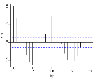
(c) ACF

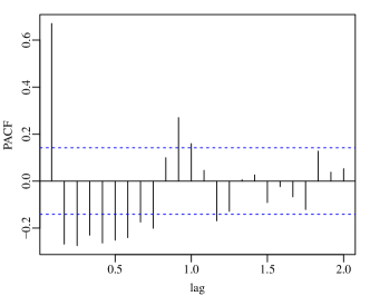
(d) PACF

Figure 2: Observed RH time series in Brasilia, Brazil.

Relative humidity is an important climate quantity which influences the weather in several ways. The Brazilian capital, Brasilia, is situated in the Center-West Region of Brazil, approximately at latitude 15° 48’ south and longitude 48° 55’ west. This particular region in Brazil is plagued by a punishing dry season (Coutinho, 2002). During the dry months, RH often attain dangerously low values, as low as 8% (measured in July, 7th, 2016 at the Jucelino Kubitshek airport in Brasilia). According to the data from the Instituto Nacional de Meteorologia (INMET - Brazilian National Institute of Meteorological Research), the average annual precipitation in Brasilia is approximately 1500 mm, but from May to September it is specially dry, with a monthly average precipitation of only 13.2 mm (corresponding to about 6% of the annual average).

The time series we shall analyze represent the monthly average RH registered in the aforementioned station from January 2000 to December 2016, yielding a sample size $n=204$. However, the last $12$ observations have been reserved for forecasting comparison. The data is freely available at INMET’s website (http://www.inmet.gov.br). Figure 2 presents the time series plot (Figure 2(a)) and the seasonal component in the data (Figure 2(b)), sample autocorrelation (ACF) (Figure 2(c)) and sample partial autocorrelation (PACF) functions (Figure 2(d)).

From the Figures 2(a) and 2(b) we observe a clear seasonal component. There are several ways to account for this monthly seasonal component. We shall consider a simple harmonic regression approach (Bloomfield, 2013), by introducing the following covariates: $x_{t}=\big{(}\sin(2\pi t/12),\cos(2\pi t/12)\big{)},\quad\mbox{for }\ t\in\{1,\dots,n\}$. With the logit as link function, using the three-stage iterative Box-Jenkins methodology (Box et al., 2008) to select the fitted model, we successfully modeled the data using a KARMA$(5,4)$ model with the covariates given above. Table 3 brings the fitted KARMA model while Figure 4 brings some residual diagnostic plots. Figure 3(a) presents the residual plot against time. From this plot we observe no distinct pattern overtime and the typical white noise behavior for the residuals. Figure 3(b) shows the plot of the normal against the empirical quantiles. An approximately straight line, as seen in the plot, is an indication that the residuals are approximately normally distributed. Finally the ACF and PACF shown in Figures 3(c) and 3(d), respectively, can help to visually verify the residual white noise hypothesis, which was also test through the Ljung-Box test shown in Table 3. All plots and tests indicate that the fitted model can be safely used for out-of-sample forecasting.

Table 3: Fitted KARMA model for relative humidity data.

Parameter	Estimate	Std. Error	$z$ stat.	${\rm Pr}(>|z|)$
$\alpha$	$0.8322$	$0.1670$	$4.9832$	$0.0000$
$\phi_{1}$	$1.2100$	$0.1242$	$9.7410$	$0.0000$
$\phi_{2}$	$-2.0237$	$0.1196$	$16.9168$	$0.0000$
$\phi_{3}$	$1.2470$	$0.1600$	$7.7932$	$0.0000$
$\phi_{4}$	$-1.0480$	$0.1093$	$9.5841$	$0.0000$
$\phi_{5}$	$0.2150$	$0.0840$	$2.5603$	$0.0105$
$\theta_{1}$	$-1.1076$	$0.1396$	$7.9345$	$0.0000$
$\theta_{2}$	$1.8808$	$0.1773$	$10.6099$	$0.0000$
$\theta_{3}$	$-0.8707$	$0.1759$	$4.9500$	$0.0000$
$\theta_{4}$	$0.8122$	$0.1428$	$5.6866$	$0.0000$
$\varphi$	$10.8870$	$0.0741$	$146.8605$	$0.0000$
$\beta_{1}$	$0.4134$	$0.0319$	$12.9428$	$0.0000$
$\beta_{2}$	$0.4465$	$0.0358$	$12.4810$	$0.0000$
AIC=$-487.8898$
Ljung-Box ($\text{lag}=20$): $Q=22.5520$ ($p$-value=$0.3113$)

(a) Quantile residual

(b) QQ-plot

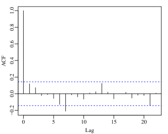
(c) Residual ACF

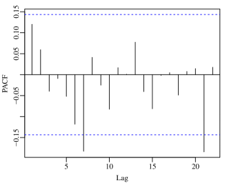
(d) Residual PACF

Figure 3: Diagnostic plots of the fitted KARMA model for relative humidity data based on the quantile residuals.

Figure 4: Out-of-sample forecasting comparison.

The out-of-sample forecast of the adjusted KARMA model is presented in Figure 4. We observe that the forecast was able to capture the distinctive seasonal pattern present in the actual data. Figure 4 also shows the forecast values for the fitted $\beta$ARMA(5,4), with the same order of the best KARMA model, and the $\beta$ARMA(2,1) which was the best $\beta$ARMA model. In order to have a better comparison we present some goodness-of-fit measures. The mean square error (MSE) and mean absolute percentage error (MAPE) between the actual data ($y_{n+h}$) and out-of-sample predicted ($\widehat{\mu}_{n+h}$) values, for $h=1,\ldots,12$, of the fitted models are presented in Table 4. We note that the proposed model outperforms the $\beta$ARMA model in both measures.

Table 4: Forecasting performance comparison among different models.

	KARMA$(5,4)$	$\beta$ARMA$(5,4)$	$\beta$ARMA$(2,1)$
MSE	$0.0050$	$0.0060$	$0.0053$
MAPE	$0.0961$	$0.1133$	$0.0989$

7 Conclusions

In this work we introduced a new class of dynamic regression models for double bounded time series. More specifically, in the proposed KARMA$(p,q)$ models, the conditional median of the Kumaraswamy distributed variable is assumed to follow a dynamic model involving covariates, an ARMA structure, unknown parameters and a link function. Inference regarding KARMA model parameters is discussed and a conditional maximum likelihood approach is fully developed. In particular, closed expression for the score vector and the conditional Fisher information matrix are obtained. The conditional maximum likelihood approach is shown to produce consistent and asymptotically normal estimates. Based on the asymptotic results, the construction of confidence intervals and hypothesis testing is discussed. Diagnostic analysis and forecasting tools are also discussed. To assess finite sample performance of the CMLE in the KARMA framework, a Monte Carlo simulation study is performed. The simulation study showed that the CMLE performs very well even for small sample sizes. To exemplify its usefulness, an application of the KARMA model to monthly relative humidity data from Brasilia, the Brazilian capital city, is presented and discussed.

An R implementation of the KARMA model

An implementation in R language (R Development Core Team, 2017) to fit the KARMA model is available at http://www.ufsm.br/bayer/karma.zip.

Appendix

In this appendix we present some technical lemmas and provide an outline of the proof of Theorem 3.1.

Appendix A Lemma 1

Let $Y_{t}$ be a random variable whose distribution given $\mathscr{F}_{t-1}$ is $K(\mu_{t},\varphi)$. Then

$$\mathds{E}\Big{[}\log(1-Y_{t}^{\varphi})|\mathscr{F}_{t-1}\Big{]}=-\frac{1}{\delta_{t}}.$$

Furthermore, if $\frac{\partial\ell_{t}}{\partial\mu_{t}}$ is given by (7), then $\mathds{E}\Big{(}\frac{\partial\ell_{t}}{\partial\mu_{t}}|\mathscr{F}_{t-1}\Big{)}=0$.

Proof: Let $f_{\mu_{t}}$ be the density of $Y_{t}$, we have

$$\mathds{E}\Big{[}\log(1-Y_{t}^{\varphi})|\mathscr{F}_{t-1}\Big{]}=\int_{0}^{1}\log(1-y^{\varphi})f_{\mu_{t}}(y)dy.$$

Expanding $\log(1-y^{\varphi})$ into a power series around 0, we obtain

$$\log(1-y^{\varphi})=-\sum_{k=1}^{\infty}\frac{(y^{\varphi})^{k}}{k}=-\sum_{k=1}^{\infty}\frac{y^{k\varphi}}{k},$$

from which it follows that

$$\int_{0}^{1}\log(1-y^{\varphi})f_{\mu_{t}}(y)dy=-\int_{0}^{1}\sum_{k=1}^{\infty}\frac{y^{k\varphi}}{k}f_{\mu_{t}}(y)dy=-\sum_{k=1}^{\infty}\frac{1}{k}\int_{0}^{1}y^{k\varphi}f_{\mu_{t}}(y)dy=-\sum_{k=1}^{\infty}\frac{1}{k}\mathds{E}(Y_{t}^{k\varphi}|\mathscr{F}_{t-1}).$$

From Proposition 3.2 in Mitnik (2013), it follows that, conditionally to $\mathscr{F}_{t-1}$, $Y_{t}^{k\varphi}\sim K(k,\delta_{t})$ and hence

$$\mathds{E}\Big{[}\log(1-Y_{t}^{\varphi})\big{|}\mathscr{F}_{t-1}\Big{]} =-\delta_{t}\sum_{k=1}^{\infty}\frac{1}{k}\texttt{B}\left(k+1,\delta_{t}\right).$$

Since $\Gamma(k+1)=k\Gamma(k)$, for positive integer $k$, for $a>0$

$$\frac{1}{k}\texttt{B}(k+1,a)=\frac{\Gamma(k+1)\Gamma(a)}{\Gamma(a+k+1)}=\frac{k!\Gamma(a)}{k\Gamma(a)\prod_{i=0}^{k}(a+i)}=\frac{(k-1)!}{\prod_{i=0}^{k}(a+i)}=\frac{1}{a(a+1)}\binom{a+k}{a+1}^{-1}.$$

Hence

$$\mathds{E}\Big{[}\log(1-Y_{t}^{\varphi})\big{|}\mathscr{F}_{t-1}\Big{]}=-\frac{1}{\delta_{t}+1}\sum_{k=1}^{\infty}\binom{\delta_{t}+k}{\delta_{t}+1}^{-1}=-\frac{1}{\delta_{t}+1}\bigg{[}1+\frac{1}{\delta_{t}}\bigg{]}=-\frac{1}{\delta_{t}},$$ (19)

which is the desired result. The last assertion is a consequence of (19) and (7). ∎

Appendix B Lemma 2

If $Y_{t}$ is a random variable for which $Y_{t}|\mathscr{F}_{t-1}\sim K(\mu_{t},\varphi)$, then (for $\delta_{t}\not\in\{1,2\}$)

$$\mathds{E}\bigg{(}\frac{Y_{t}^{\varphi}\log(Y_{t})}{1-Y_{t}^{\varphi}}\bigg{|}\mathscr{F}_{t-1}\bigg{)}=\frac{1-\psi(\delta_{t}+1)-\kappa}{(\delta_{t}-1)\varphi}$$

and

$$\mathds{E}\bigg{(}\frac{Y_{t}^{\varphi}\log(Y_{t})^{2}}{(1-Y_{t}^{\varphi})^{2}}\bigg{|}\mathscr{F}_{t-1}\bigg{)}=\frac{\delta_{t}\left(\psi(\delta_{t})\big{[}\psi(\delta_{t})+2(\kappa-1)\big{]}-\psi^{\prime}(\delta_{t})+k_{0}\right)}{(\delta_{t}-2)(\delta_{t}-1)\varphi^{2}},$$

where $\psi:(0,\infty)\rightarrow\mathds{R}$ is the digamma function defined as $\psi(z)=\frac{d}{dz}\log\big{(}\Gamma(z)\big{)}$, $\psi^{\prime}(z)=\frac{d}{dz}\psi(z)$ is the trigamma function, $\kappa=0.5772156649\dots$ is the Euler-Mascheroni constant (Gradshteyn and Ryzhik, 2007) and $k_{0}=\pi^{2}/6+\kappa^{2}-2\kappa$.

Proof: We have

$$\mathds{E}\bigg{(}\frac{Y_{t}^{\varphi}\log(Y_{t})}{1-Y_{t}^{\varphi}}\bigg{|}\mathscr{F}_{t-1}\bigg{)}=\varphi\delta_{t}\int_{0}^{1}y^{2\varphi-1}\log(y)(1-y^{\varphi})^{\delta_{t}-2}dy.$$

Upon expanding $(1-y^{\varphi})^{\delta_{t}-2}$ into its binomial series, we have $(1-y^{\varphi})^{\delta_{t}-2}=\displaystyle{\sum_{k=0}^{\infty}}(-y^{\varphi})^{k}\binom{\delta_{t}-2}{k}$ and

$$\mathds{E}\bigg{(}\frac{Y_{t}^{\varphi}\log(Y_{t})}{1-Y_{t}^{\varphi}}\bigg{|}\mathscr{F}_{t-1}\bigg{)} =\varphi\delta_{t}\sum_{k=0}^{\infty}(-1)^{k}\binom{\delta_{t}-2}{k}\int_{0}^{1}y^{\varphi(k+2)-1}\log(y)dy$$

$$=\varphi\delta_{t}\sum_{k=0}^{\infty}(-1)^{k}\binom{\delta_{t}-2}{k}\bigg{[}-\frac{1}{\varphi^{2}(k+2)^{2}}\bigg{]}=-\frac{\delta_{t}}{\varphi}\sum_{k=0}^{\infty}\frac{(-1)^{k}}{(k+2)^{2}}\binom{\delta_{t}-2}{k}.$$

To evaluate the series above, we change the index to $i=k+2$ and rewrite

$$\sum_{k=0}^{\infty}\frac{(-1)^{k}}{(k+2)^{2}}\binom{\delta_{t}-2}{k} =\sum_{i=2}^{\infty}\frac{(-1)^{i-2}}{i}\bigg{[}\frac{1}{i}\binom{\delta_{t}-2}{i-2}\bigg{]}=\sum_{k=1}^{\infty}\frac{(-1)^{i-2}}{i}\bigg{[}\frac{(i-1)}{\delta_{t}(\delta_{t}-1)}\binom{\delta_{t}}{i}\bigg{]}$$

$$=\frac{1}{\delta_{t}(\delta_{t}-1)}\bigg{[}\sum_{i=1}^{\infty}(-1)^{i}\binom{\delta_{t}}{i}-\sum_{i=1}^{\infty}\frac{(-1)^{i}}{i}\binom{\delta_{t}}{i}\bigg{]}.$$

The result now follows by the Newton’s series for the digamma function (formula 8.363.8 in Gradshteyn and Ryzhik, 2007, with $n=0$), that is,

$$\psi(s+1)+\kappa=-\sum_{k=1}^{\infty}\frac{(-1)^{k}}{k}\binom{s}{k},$$

and the identity $\sum_{k=1}^{\infty}(-1)^{k}\binom{n}{k}=-1$. Similar technique yields

$$\mathds{E}\bigg{(}\frac{Y_{t}^{\varphi}\log(Y_{t})^{2}}{(1-Y_{t}^{\varphi})^{2}}\bigg{|}\mathscr{F}_{t-1}\bigg{)} =\varphi\delta_{t}\sum_{k=0}^{\infty}(-1)^{k}\binom{\delta_{t}-3}{k}\int_{0}^{1}y^{\varphi(k+2)-1}\log(y)^{2}dy$$

$$=\varphi\delta_{t}\sum_{k=0}^{\infty}(-1)^{k}\binom{\delta_{t}-3}{k}\bigg{[}\frac{2}{\varphi^{3}(k+2)^{3}}\bigg{]}=\frac{2\delta_{t}}{\varphi^{2}}\sum_{k=0}^{\infty}\frac{(-1)^{k}}{(k+2)^{3}}\binom{\delta_{t}-3}{k}.$$

The result now follows by similar argument as the previous case and from the Newton’s series for the digamma and $\psi^{\prime}(x)$ functions (formula 8.363.8 in Gradshteyn and Ryzhik, 2007, with $n=0,1$), that is,$\psi^{\prime}(x)=\sum_{k=0}^{\infty}\frac{1}{(x+k)^{2}}$. ∎

Appendix C Proof of Theorem 3.1

Proof: In order to obtain the results, we only need to check that assumptions 2.1-2.5 from Andersen (1970) are fulfilled. Assumption 2.1 follows from Section 3.1. Assumption 2.2 follow from standard results for ARMA models with covariates (Hannan, 1973). To show that Assumption 2.3 holds, observe that, for small $\delta$ in a neighborhood of 0, the argument for the variance can be written as (recall that conditionally on the past, $y_{t}$’s are independent)

$$\sum_{t=m}^{n} \ell_{t}(\mu_{t},\varphi+\delta)-\ell_{t}(\mu_{t},\varphi)=\sum_{t=m}^{n}\delta\log(y_{t})+J_{\varphi+\delta}\log(1-y_{t}^{\varphi+\delta})-J_{\varphi}\log(1-y_{t}^{\varphi})+C_{t}$$

where $J_{x}=\log\Big{(}\log\big{(}0.5/\log(1-\mu_{t}^{x})\big{)}\Big{)}$ and $C_{t}$ are (non-random) real constants. The terms $\log(y_{t})$, $\log(1-y_{t}^{\varphi+\delta})$ and $\log(1-y_{t}^{\varphi})$ can be shown to be continuous functions of their arguments so that the result follows (see Andersen, 1970). Assumption 2.3 are satisfied by the definition of the KARMA model and the results on Section 3. Assumption 2.4 is a consequence of Lemma 1 in A and the final condition follows from the assumptions on the design (covariate) matrix and Section 3.2. ∎

References

References

- Akaike (1974) Akaike, H., 1974. A new look at the statistical model identification. IEEE Transactions on Automatic Control 19 (6), 716–723.
- Allen et al. (1998) Allen, R. G., Pereira, L. S., Raes, D., Smith, M., 1998. Crop evapotranspiration: Guidelines for computing crop water requirements. Tech. rep., Food and Agriculture Organization of the United Nations.
- Andersen (1970) Andersen, B. A., 1970. Asymptotic properties of conditional maximum-likelihood estimators. Journal of the Royal Statistic Society Serie B 32 (1), 283–301.
- Ansley and Newbold (1980) Ansley, C. F., Newbold, P., 1980. Finite sample properties of estimators for autorregressive moving average models. Journal of Econometrics 13 (2), 159–183.
- Arnold et al. (2012) Arnold, J. G., Kiniry, J. R., Srinivasan, R., Williams, J. R., Haney, E. B., Neitsch, S., 2012. Soil & water assessment tools. Tech. rep., Texas Water Resurces Institute.
- Bayer and Cribari-Neto (2013) Bayer, F., Cribari-Neto, F., 2013. Bartlett corrections in beta regression models. Journal of Statistical Planning and Inference 143 (3), 531–547.
- Benjamin et al. (2003) Benjamin, M. A., Rigby, R. A., Stasinopoulos, D. M., 2003. Generalized autoregressive moving average models. Journal of the American Statistical Association 98 (461), 214–223.
- Bloomfield (2013) Bloomfield, P., 2013. Fourier Analysis of Time Series: An Introduction, 2nd Edition. Wiley-Interscience, p. 288.
- Box et al. (2008) Box, G., Jenkins, G. M., Reinsel, G., June 2008. Time series analysis: forecasting and control. Hardcover, John Wiley & Sons.
- Brockwell and Davis (1991) Brockwell, P. J., Davis, R. A., 1991. Time Series: Theory and Methods, 2nd Edition. Springer-Verlag.
- Chuang and Yu (2007) Chuang, M.-D., Yu, G.-H., 2007. Order series method for forecasting non-Gaussian time series. Journal of Forecasting 26 (4), 239–250.
- Collishonn et al. (2007) Collishonn, W., Allasia, D., Da Silva, B. C., Tucci, C. E. M., 2007. The MGB-IPH model for large-scale rainfall-runoff modelling. Hydrological Sciences Journal 52 (5), 878–895.
- Coutinho (2002) Coutinho, L. M., 2002. Eugen Warming e o Cerrado brasileiro: um século depois. UNESP, São Paulo, Ch. O bioma Cerrado, pp. 77–92.
- Cox and Reid (1987) Cox, D. R., Reid, N., 1987. Parameter orthogonality and approximate conditional inference. Journal of the Royal Statistical Society. Series B 49 (1), 1–39.
- Cribari-Neto and Zeileis (2010) Cribari-Neto, F., Zeileis, A., 2010. Beta regression in R. Journal of Statistical Software 34 (2).
- da Silva et al. (2011) da Silva, C., Migon, H., Correia, L., 2011. Dynamic bayesian beta models. Computational Statistics & Data Analysis 55 (6), 2074–2089.
- Dunn and Smyth (1996) Dunn, P. K., Smyth, G. K., 1996. Randomized quantile residuals. Journal of Computational and Graphical Statistics 5 (3), 236–244.
- Falagas et al. (2008) Falagas, M. E., Theocharis, G., Spanos, A., Vlara, L. A., Issaris, E. A., Panos, G., Peppas, G., 2008. Effect of meteorological variables on the incidence of respiratory tract infections. Respiratory Medicine 102 (5), 733 – 737.
- Ferrari and Cribari-Neto (2004) Ferrari, S. L. P., Cribari-Neto, F., 2004. Beta regression for modelling rates and proportions. Journal of Applied Statistics 31 (7), 799–815.
- Fletcher and Ponnambalam (1996) Fletcher, S., Ponnambalam, K., 1996. Estimation of reservoir yield and storage distribution using moments analysis. Journal of Hydrology 182 (1–4), 259–275.
- Fokianos and Kedem (2004) Fokianos, K., Kedem, B., 2004. Partial likelihood inference for time series following generalized linear models. Journal of Time Series Analysis 25 (2), 173–197.
- Ganji et al. (2006) Ganji, A., Ponnambalam, K., Khalili, D., Karamouz, M., 2006. Grain yield reliability analysis with crop water demand uncertainty. Stochastic Environmental Research and Risk Assessment 20 (4), 259–277.
- Gradshteyn and Ryzhik (2007) Gradshteyn, I. S., Ryzhik, I. M., 2007. Table of integrals, series, and products, 7th Edition. Academic Press.
- Greene (2011) Greene, W. H., 2011. Econometric Analysis, 7th Edition. Pearson.
- Guolo and Varin (2014) Guolo, A., Varin, C., 03 2014. Beta regression for time series analysis of bounded data, with application to Canada Google Flu Trends. The Annals of Applied Statistics 8 (1), 74–88.
- Gupta and Nadarajah (2004) Gupta, A. K., Nadarajah, S., 2004. Handbook of Beta Distribution and Its Applications. CRC Press.
- Hannan (1973) Hannan, E., 1973. The asymptotic theory of linear time-series models. Journal of Applied Probability 10 (1), 130–145.
- Hannan and Quinn (1979) Hannan, E. J., Quinn, B. G., 1979. The determination of the order of an autoregression. Journal of the Royal Statistical Society. Series B 41 (2), 190–195.
- John (2015) John, O. O., 2015. Robustness of quantile regression to outliers. American Journal of Applied Mathematics and Statistics 3 (2), 86–88.
- Jones (2009) Jones, M., 2009. Kumaraswamy’s distribution: A beta-type distribution with some tractability advantages. Statistical Methodology 6 (1), 70–81.
- Kedem and Fokianos (2002) Kedem, B., Fokianos, K., 2002. Regression models for time series analysis. John Wiley & Sons.
- Koutsoyiannis and Xanthopoulos (1989) Koutsoyiannis, D., Xanthopoulos, T., 1989. On the parametric approach to unit hydrograph identification. Water Resources Management 3 (2), 107–128.
- Kumaraswamy (1976) Kumaraswamy, P., 1976. Sinepower probability density function. Journal of Hydrology 31, 181–184.
- Kumaraswamy (1980) Kumaraswamy, P., 1980. A generalized probability density function for double-bounded random processes. Journal of Hydrology 46, 79–88.
- Lemonte et al. (2013) Lemonte, A. J., Barreto-Souza, W., Cordeiro, G. M., 2013. The exponentiated Kumaraswamy distribution and its log-transform. Brazilian Journal of Probability and Statistics 27 (1), 31–53.
- Lemonte and Bazán (2016) Lemonte, A. J., Bazán, J. L., 2016. New class of Johnson SB distributions and its associated regression model for rates and proportions. Biometrical Journal 58 (4), 727–746.
- Ljung and Box (1978) Ljung, G. M., Box, G. E. P., 1978. On a measure of lack of fit in time series models. Biometrika 65 (2), pp. 297–303.
- Lohani et al. (2012) Lohani, A., Kumar, R., Singh, R., 2012. Hydrological time series modeling: A comparison between adaptive neuro-fuzzy, neural network and autoregressive techniques. Journal of Hydrology 442, 23–35.
- Machiwal and Jha (2012) Machiwal, D., Jha, M. K., 2012. Hydrologic Time Series Analysis. Springer Netherlands.
- Mauricio (2008) Mauricio, J. A., 2008. Computing and using residuals in time series models. Computational Statistics & Data Analysis 52 (3), 1746–1763.
- McCullagh and Nelder (1989) McCullagh, P., Nelder, J., 1989. Generalized linear models, 2nd Edition. Chapman and Hall.
- Mitnik (2013) Mitnik, P. A., 2013. New properties of the Kumaraswamy distribution. Communications in Statistics-Theory and Methods 42 (5), 741–755.
- Mitnik and Baek (2013) Mitnik, P. A., Baek, S., 2013. The Kumaraswamy distribution: median-dispersion re-parameterizations for regression modeling and simulation-based estimation. Statistical Papers 54 (1), 177–192.
- Nadarajah (2008) Nadarajah, S., 2008. On the distribution of Kumaraswamy. Journal of Hydrology 348 (3–4), 568–569.
- Neyman and Pearson (1928) Neyman, J., Pearson, E. S., 1928. On the use and interpretation of certain test criteria for purposes of statistical inference. Biometrika 20A (1/2), 175–240.
- Nocedal and Wright (1999) Nocedal, J., Wright, S. J., 1999. Numerical optimization. Springer.
- Ospina and Ferrari (2012) Ospina, R., Ferrari, S. L. P., 2012. A general class of zero-or-one inflated beta regression models. Computational Statistics & Data Analysis 56, 1609–1623.
- Palm and Bayer (2017) Palm, B. G., Bayer, F. M., 2017. Bootstrap-based inferential improvements in beta autoregressive moving average model. Communications in Statistics - Simulation and Computation, 1–20 DOI: 10.1080/03610918.2017.1300268.
- Pawitan (2001) Pawitan, Y., 2001. In All Likelihood: Statistical Modelling and Inference Using Likelihood. Oxford Science publications.
- Pereira (2017) Pereira, G., 2017. On quantile residuals in beta regression. ArXiv e-prints.
- Ponnambalam et al. (2001) Ponnambalam, K., Seifi, A., Vlach, J., 2001. Probabilistic design of systems with general distributions of parameters. International Journal of Circuit Theory and Applications 29 (6), 527–536.
- Press et al. (1992) Press, W., Teukolsky, S., Vetterling, W., Flannery, B., 1992. Numerical recipes in C: The art of scientific computing, 2nd Edition. Cambridge University Press.
- R Development Core Team (2017) R Development Core Team (2017). R: A Language and Environment for Statistical Computing. R Foundation for Statistical Computing, Vienna, Austria, ISBN 3-900051-07-0.
- Rao (1948) Rao, C., 1948. Large sample tests of statistical hypotheses concerning several parameters with applications to problems of estimation. Mathematical Proceedings of the Cambridge Philosophical Society 44 (1), 50–57.
- Rocha and Cribari-Neto (2009) Rocha, A. V., Cribari-Neto, F., 2009. Beta autoregressive moving average models. Test 18 (3), 529–545.
- Salas et al. (1997) Salas, J. D., Delleur, J., Yevjevich, V., Lane, W., 1997. Applied Modeling of Hydrologic Time Series, 4th Edition. Water Resources Pubns.
- Schwarz (1978) Schwarz, G., 1978. Estimating the dimension of a model. The Annals of Statistics 6 (2), 461–464.
- Seifi et al. (2000) Seifi, A., Ponnambalam, K., Vlach, J., 2000. Maximization of manufacturing yield of systems with arbitrary distributions of component values. Annals of Operations Research 99 (1), 373–383.
- Shuttleworth (1993) Shuttleworth, W. J., 1993. Handbook of Hydrology. McGraw-Hill, New York, Ch. Evaporation, pp. 4.1–4.53.
- Silveira (2002) Silveira, A., 2002. Problems of modern urban drainage in developing countries. Water Science and Technology 45 (7), 31–40.
- Simas et al. (2010) Simas, A. B., Barreto-Souza, W., V., R. A., 2010. Improved estimators for a general class of beta regression models. Computational Statistics & Data Analysis 2, 348–366.
- Souza and Cribari-Neto (2015) Souza, T. C., Cribari-Neto, F., 2015. Intelligence, religiosity and homosexuality non-acceptance: Empirical evidence. Intelligence 52, 63–70.
- Sundar and Subbiah (1989) Sundar, V., Subbiah, K., 1989. Application of double bounded probability density function for analysis of ocean waves. Ocean Engineering 16 (2), 193–200.
- Terrell (2002) Terrell, G. R., 2002. The gradient statistic. Computing Science and Statistics 34, 206–215.
- Tiku et al. (2000) Tiku, M. L., Wong, W.-K., Vaughan, D. C., Bian, G., 2000. Time series models in non-normal situations: Symmetric innovations. Journal of Time Series Analysis 21 (5), 571–596.
- Valipour et al. (2013) Valipour, M., Banihabib, M. E., Behbahani, S. M. R., 2013. Comparison of the ARMA, ARIMA, and the autoregressive artificial neural network models in forecasting the monthly inflow of dez dam reservoir. Journal of Hydrology 476, 433–441.
- Wald (1943) Wald, A., 1943. Tests of statistical hypotheses concerning several parameters when the number of observations is large. Transactions of the American Mathematical Society 54, 426–482.
- Zhang et al. (2016) Zhang, D. S., Zhang, X., Ouyang, Y. H., Zhang, L., Ma, S. L., He, J., 2016. Incidence of allergic rhinitis and meteorological variables: Non-linear correlation and non-linear regression analysis based on Yunqi theory of chinese medicine. Chinese Journal of Integrative Medicine DOI: 10.1007/s11655-016-2588-9.