Results

A Toolkit For Steady States of Nonlinear Wave Equations:
Continuous Time Nesterov and Exponential Time Differencing Schemes

Several methods exist for finding ground (as well as excited) states of nonlinear waves equations. In this paper we first introduce two modifications of the so-called accelerated imaginary-time evolution method (AITEM). In our first modification, time integration of the underlying gradient flow is done using exponential time differencing instead of using more standard methods. In the second modification, we present a generalization of the gradient flow model, motivated by the work of Nesterov, as well as that of Candes and collaborators. Additionally, we consider combinations of these methods with the so-called spectral renormalization scheme. Finally, we apply these techniques to the so-called Squared Operator Method, enabling convergence to excited states. Various examples are shown to illustrate the effectiveness of these new schemes, comparing them to standard ones established in the literature. In most cases, we find significant reductions in the number of iterations needed to reach convergence.

I.  Introduction

In models stemming from nonlinear optics and atomic physics, it is customary to seek a Hamiltonian description of the dynamics, e.g., for the envelope of optical pulses or for the wavefunction of quantum systems that follows a Schrödinger type partial differential equation. If, in addition, nonlinear effects are contributing, e.g., either because of the so-called Kerr effect in optics [hasegawa, kivshar] or because of the mean-field interaction of bosonic atoms [GP, becbook1, becbook2, rcg:BEC_BOOK, rcg:BEC_book2], then the prototypical model becomes the nonlinear Schrödinger (NLS) equation. The NLS [ablowitz, abl2, ablowitz1, sulem, chap01:bourgain] is a dispersive nonlinear partial differential equation (PDE) that has been essential in understanding some of the most groundbreaking results in the physics of such systems. Additional areas of application include, but are not limited to Langmuir waves in plasmas [zakh1, zakh2], deep water and freak/rogue waves, [benjamin, onofrio], as well as more broadly in fluid mechanics [infeld].

In its canonical form, the equation reads:

$$\begin{array}[]{rcl}i\partial_{t}u=-\frac{1}{2}\nabla^{2}u+g|u|^{2}u,\end{array}$$ (1)

where $u$ is the complex field and $g$ is a constant. Physically, $u$ may represent the envelope of the electric field in optics, the amplitude of water waves or the wavefunction of a Bose-Einstein condensate (BEC) and is the main object whose spatio-temporal evolution we are interested in probing. Very commonly in the above areas, we are interested in identifying standing wave solutions of Eq. (1) in the form: $u(x,t)=\psi(x)e^{-i\mu t}$ which, in turn, leads to the time-independent form of the equation: rcl ∇^2 ψ-V(x) ψ+ σ—ψ—^2 ψ+ μψ& =  0. The parameter $\mu$ is associated to the frequency of the solution and is referred to as the propagation constant in optics or the chemical potential in atomic BECs. This steady state problem constitutes a subject of wide exploration, to which a broad and diverse number of studies has been devoted. Both the ground and the excited states in this elliptic, nonlinear PDE problem are of interest. It should be noted that given the importance of the subject entire books have been dedicated to the analysis of associated numerical methods [yangbook].

Our aim in the present work is to add some useful twists to this extensive literature, based on recent computational developments in other areas (including the time stepping of ordinary and partial differential equations, and the development of schemes relevant for the iterative convergence of functional extremization). Our main contribution is to propose iterative schemes, based on the continuous time variant of Nesterov’s method [5, 4, MJ], for finding stationary states of Eq. (1). The structure of our presentation is as follows. Given the extensive literature on the subject related to the NLS model, we start by presenting in section II some of the most popular methods that do not resort to the use of the Jacobian (i.e., Newton-type methods); the latter, and accelerated variants thereof, merit their own independent examination that is deferred to a future stage. Then, we present in section III our proposed “twists” based on the above recent computational developments and their implementation in Eq. (1). In section IV we compare the results of the newly proposed variants with the more standardly used methods. Finally, in section V, we summarize our findings and present some challenges for the future.

II.  Earlier Methods for Calculating Ground States

In this section we discuss two among the most widely used, previously developed methods, AITEM [2] and the Spectral Renormalization method [3], for identifying ground states of the steady state problem within the NLS equation.

A.  AITEM

Eq. (1) can be recast in the variational form

rcl min_ψ ∫— ∇ψ—^2 +V(x)— ψ—^2 - σ2 — ψ—^4   dx &   subject to    ∫— ψ—^2   dx =P, where the first integral is the field-theoretic energy $E(\psi)$ of the system and the second integral fixes the number of particles (in the atomic case) or the power –hence the symbol– in the optical case to be $P$ .

Using a Lagrange multiplier, we can directly incorporate the relevant constraint. The resulting gradient flow is then given by rcl ˙ψ & = ∇^2 ψ-V(x) ψ+ σ—ψ—^2 ψ+ μψ. In tradional variational problems, $P$ is typically known and $\mu$ unknown i.e. the constraint is a given but the Lagrange multiplier must be identified. In this case, we can let $\mu=\mu(t)$ be a function of time such that $\mu(t)$ converges to the true value of the Lagrange multiplier as $t\to\infty$. One such choice of $\mu(t)$ was given by Yang and Lakoba [2] as

$$\mu(t)=-\frac{\langle L\psi,\psi\rangle}{\langle\psi,\psi\rangle}$$ (2)

where the inner products represent the standard $L^{2}$ inner product and $L=\nabla^{2}\psi-V(x)\psi+\sigma|\psi|^{2}\psi$; if one thinks of $\mu$ as an eigenvalue then this is the standard Rayleigh quotient. Because $\psi=0$ is always a solution of the NLS, one must still include the constraint $\int|\psi|^{2}\;dx=P$ to ensure the evolution does not go to the trivial solution. If one applies, say, the standard Euler method to (A) and also adds a preconditioner $M$, then one gets the AITEM scheme: rcl M&  =   c-∇^2
μ_n   =   ⟨M-1L ψn, ψn⟩⟨M-1ψn, ψn⟩
~ψ_n+1   =   ψ_n - M^-1(L ψ_n + μ_n ψ_n) Δt
ψ_n+1  =  ~ψ_n+1 P⟨~ψn+1,~ψn+1⟩. The fourth equation ensures that the number of particles (the constraint $\int|\psi|^{2}\;dx=P$) is satisfied after each iteration. We remark that the parameter $c$ is a positive number which must be chosen a priori.

B.  Spectral Renormalization

An alternative method applicable to the NLS for general nonlinearity $N$ is the so-called spectral renormalization method, addressing problems of the form: rcl ∇^2 ψ-V(x) ψ+ N(—ψ—^2)ψ+ μψ& =  0 Unlike before, here we think of $\mu$ as a fixed constant. If we take the Fourier transform (denoted by ${\cal F}$) of this equation we obtain

$$-|\textbf{k}|^{2}\hat{\psi}+\mathcal{F}[-V(x)\psi+N(|\psi|^{2})\psi]+\mu\hat{\psi}=0$$

and solving for $\hat{\psi}$ yields

$$\hat{\psi}=\frac{\mathcal{F}[-V(x)\psi+N(|\psi|^{2})\psi]}{|\textbf{k}|^{2}-\mu}$$

Thinking of this as a fixed point iteration method

$$\hat{\psi}_{n+1}=\frac{\mathcal{F}[-V(x)\psi_{n}+N(|\psi_{n}|^{2})\psi_{n}]}{|\textbf{k}|^{2}-\mu}$$

we might expect this to converge to a ground state. However numerical experiments have shown that it tends to converge to zero or diverge without bound.

To get around this problem, Ablowitz and Musslimani [3] suggested that one should include a renormalization factor $\lambda$, which is determined by the iteration procedure itself. Letting $\psi=\lambda\phi$, $\hat{\psi}=\lambda\hat{\phi}$, plugging these into the NLS equation, and repeating gives

$$\hat{\phi}=\frac{\mathcal{F}[-V(x)\phi+N(|\lambda\phi|^{2})\phi]}{|\textbf{k}|^{2}-\mu}$$

If we now multiply the previous equation by $\hat{\phi}$ and integrate we get an algebraic condition on $\lambda$:

$$\langle\hat{\phi},\hat{\phi}\rangle-\langle\hat{\phi},\frac{\mathcal{F}[-V(x)\phi+N(|\lambda\phi|^{2})\phi]}{|\textbf{k}|^{2}-\mu}\rangle=0$$

Since $\lambda$ is just a scalar, we see that it is determined by the above equation. We then have the scheme: rcl 0 & =  ⟨^ϕ_n , ^ϕ_n ⟩- ⟨^ϕ_n , F [-V(x) ϕn+ N(—λnϕn—2)ϕn]—k—2- μ ⟩
^ϕ_n+1 =  F [-V(x) ϕn+ N(—λnϕn—2)ϕn]—k—2- μ

One drawback of the scheme as written is that if $\mu$ is not negative then the iteration leads to division by zero. In [3], it was thus suggested that the term $r\psi$ be added and subtracted to the NLS equation; if one then repeats the argument, a scheme where division by zero does not occur can be devised. This scheme, the Spectral Renormalization method, is given by rcl 0 & =  ⟨^ϕ_n , ^ϕ_n ⟩- ⟨^ϕ_n , (r + μ)^ϕnr+—k—2 + F [-V(x) ϕn+ N(—λnϕn—2)ϕn]r+—k—2 ⟩
^ϕ_n+1 =  (r + μ)^ϕnr+—k—2 + F [-V(x) ϕn+ N(—λnϕn—2)ϕn]r+—k—2. where $r$ is some positive parameter which must be chosen before the iteration begins.

III.  Proposed Twists

In this section we propose a number of modifications and extensions of AITEM and Spectral Renormalization.

A.  Exponential Time Differencing

The first of these new methods is simply a different way of time-stepping the gradient flow equation. Namely, using the first-order exponential time differencing scheme [7, 8] instead of Euler’s method.

More specifically, consider Eq. (A) again. By taking the Fourier transform of both sides we arrive at

$$\hat{\psi}_{t}=-|\textbf{k}|^{2}\hat{\psi}+\mathcal{F}[-V(x)\psi+\sigma|\psi|^{2}\psi]+\mu\hat{\psi}$$

Applying the first order exponential time differencing scheme to this equation we get

$$\hat{\psi}_{n+1}=e^{-|\textbf{k}|^{2}h}\hat{\psi}_{n}+\frac{e^{-|\textbf{k}|^{2}h}-1}{-|\textbf{k}|^{2}}[\mathcal{F}[-V(x)\psi_{n}+\sigma|\psi_{n}|^{2}\psi_{n}]+\mu\hat{\psi}_{n}]$$

However, some care is needed in dealing with the term $\frac{e^{-|\textbf{k}|^{2}h}-1}{-|\textbf{k}|^{2}}$ so that division by zero and catastrophic cancellation do not occur. We refer the reader to the insightful work of Kassam and Treffethen [8] in which they propose to use the Cauchy integral formula to calculate this expression and include a Matlab code for implementing this at the end.

Now, we have to impose the constraint $\int|\psi|^{2}dx=P$. We proceed in a similar fashion as AITEM: rcl μ_n &   =   ⟨L ^ψn, ^ψn⟩⟨^ψn, ^ψn⟩
~^ψ_n+1   =   e^-—k—^2h^ψ_n + e-—k—2h- 1-—k—2[F [- V(x) ψ_n+ σ—ψ_n —^2ψ_n] + μ_n ^ψ_n]
^ψ_n+1  =  ~^ψ_n+1 P⟨~^ψn+1,~^ψn+1⟩ where $L\hat{\psi}=-|\textbf{k}|^{2}\hat{\psi}+\mathcal{F}[-V(x)\psi+\sigma|\psi|^{2}\psi]$ and $h=\Delta t$, the proposed effective time step. We will refer to this scheme as ETD for the remainder of the paper. Our main motivation for proposing this scheme is that it does not need a preconditioner like that in AITEM; in some sense, Duhamel’s formula itself –incorporating the integration of the Laplacian term– is a preconditioner. We also expect that if the potential stiffness is due to the Laplacian term, then this method should perform quite well.

If the stiffness is instead concentrated in the term $V(x)\psi$ then we expect ETD and AITEM to do far more poorly. In such a case, we propose that $V(x)\psi$ should be considered the linear part and not $\nabla^{2}\psi$. Before proceeding, we remark that if one does exponential time differencing in physical space then it is difficult to compute the operator $e^{\nabla^{2}h}$. Moreover, in Fourier space it is difficult to separate $\hat{\psi}$ in $\mathcal{F}[V(x)\psi]$ from the potential; what this implies computationally is that one must choose between letting the Laplacian or the potential to be included in the linear part.

Now, staying in physical space and performing exponential time differencing based on the potential gives rcl μ_n &   =   ⟨L ψn, ψn⟩⟨ψn, ψn⟩
~ψ_n+1   =   e^-V(x) h ψ_n + e-V(x) h- 1-V(x)[∇^2 ψ_n+ σ—ψ_n —^2ψ_n + μ_n ψ_n]
ψ_n+1  =  ~ψ_n+1 P⟨~ψn+1,~ψn+1⟩ where, again, the term $\frac{e^{-V(x)h}-1}{-V(x)}$ must be interpreted appropriately. We will refer to this scheme as ETDV.

B.  Continuous Time Nesterov

Consider the variational problem of minimizing the function $F(x)$; here we are considering $F$ to be a function and not a functional. To solve this problem, one method is of course to use gradient descent. However, if $F$ is sufficiently “ill-behaved” we do not expect that gradient descent will converge easily. As an alternative, Su, Boyd, and Candes [4] were able to formulate a second order ODE which in some sense generalizes gradient descent:

$$\ddot{x}+\frac{3}{t}\dot{x}+\nabla F(x)=0$$

As discussed in their paper, this ODE is actually a continuous version of Nesterov’s (discrete) mirror descent [5]. Henceforth, we will refer to this scheme as continuous time Nesterov (CTN).

Two major differences occur between CTN and gradient descent. The first, and crucial one (since it will also enable the second as we will see), is that CTN is a second order ODE. Roughly speaking, this means that the acceleration vector, and NOT the velocity vector, points in the direction that the field is decreasing fastest (at least for large $t$). This is similar to a particle moving in the force field of a potential i.e. a related way of envisioning this ODE is to say that the particle has been given mass and has a time-dependent dissipation on which we now comment. The second major difference is the dissipation term $\frac{3}{t}\dot{x}$; thinking of a particle in a potential, we see that this term has the effect of damping the energy/momentum. However, this damping is tuned to be large at the initial time, when presumably the particle is far from the equilibrium while it decreases the closer that one (hopefully) gets to the relevant fixed point. This term is, thus, responsible for the actual convergence of the method to minima of $F$. With too little damping the method will only oscillate around the minima but with too much damping the method could be terribly inefficient.

In the work of [4], the authors suggest using a second-order center difference scheme for approximating the second derivative and a first order backward difference scheme for approximating the first derivative. Doing this and rearranging the dynamical evolution equation gives the scheme

$$x_{n+1}=(2-\frac{3}{n})x_{n}-(\Delta t)^{2}\nabla F(x_{n})-(1-\frac{3}{n})x_{n-1}$$

where we have let $t=n\Delta t$.

We remark in passing that, as was proven in [5], this scheme enjoys linear convergence, provided $F$ is strongly convex.

C.  Accelerated Continuous Time Nesterov

A principal contribution of the present work is to propose and illustrate the relevance of applying CTN not just to functions but to (field-theoretic) functionals; as far as we know, this application of CTN as a means of finding steady state solutions of a PDE has not been previously considered.

Returning to the variational problem (A), we see that CTN takes the form

$$\ddot{\psi}+\frac{3}{t}\dot{\psi}-(\nabla^{2}\psi-V(x)\psi+\sigma|\psi|^{2}\psi+\mu\psi)=0$$

where we have included the Lagrange multiplier $\mu$, and abused the overdot notation in this field-theoretic context to signify partial derivative with respect to $t$. Discretizing this as before, we arrive at

$$\psi_{n+1}=(2-\frac{3}{n})\psi_{n}+(\Delta t)^{2}(\nabla^{2}\psi-V(x)\psi+\sigma|\psi|^{2}\psi+\mu\psi)-(1-\frac{3}{n})\psi_{n-1}.$$

Since the dissipation term controls the convergence properties to a high degree, both in the work of [4] and in that of [6], much effort has been invested in trying to optimize it. In particular, it is proposed to reset time $t$ at appropriate points in the evolution so that CTN is always sufficiently damped; again, when $t$ is small there is a large amount of damping. Such a variant is the gradient restarting scheme, whereby time is reset to one when the angle between $-\nabla F(x)$ and $\dot{x}$ is greater than $90$ degrees AND a prespecified amount of time $t_{res}$ has elapsed: rcl ⟨∇F(x) , ˙x ⟩&¿ 0
t≥t_res. If we include gradient restarting into the above descritization we get

$$\psi_{n+1}=(2-\frac{3}{\tilde{n}})\psi_{n}+(\Delta t)^{2}(\nabla^{2}\psi_{n}-V(x)\psi_{n}+\sigma|\psi_{n}|^{2}\psi_{n}+\mu\psi_{n})-(1-\frac{3}{\tilde{n}})\psi_{n-1},$$

where $\tilde{n}$ starts at one and increases by one after each iteration; once the restart condition rcl ⟨∇^2 ψ_n -V(x) ψ_n + σ—ψ_n—^2 ψ_n + μψ_n     ,     ψ_n+1 - ψ_n ⟩&¿0
n ≥ n_res is met, $\tilde{n}$ is reset to one and the process repeats.

If we include a preconditioner $M$ and recall that we must normalize after each iteration, then the full method can be written as rcl M &= c - ∇^2
μ_n   =   ⟨L ψn, ψn⟩⟨ψn, ψn⟩
~ψ_n+1 = (2- 3~n)ψ_n + (Δt)^2 M^-1 (∇^2 ψ_n -V(x) ψ_n + σ—ψ_n—^2 ψ_n + μ_n ψ_n) - (1-3~n)ψ_n-1
ψ_n+1  =  ~ψ_n+1 P⟨~ψn+1,~ψn+1⟩ where, again, $\tilde{n}$ is chosen via gradient restarting. We shall refer to this scheme as Accelerated Continuous Time Nesterov (ACTN), in the fashion of AITEM.

We remark that the convergence rate of this method is unknown to us. While CTN was proven to converge linearly under strong convexity, no convergence proof is known to us of CTN with gradient restarting (though Su, Boyd, and Candes prove something similar). With the inclusion of the preconditioner and particle number normalization, it is not clear what convergence speed should be expected. To that end, the numerical experiments below suggest the ACTN will, generically, converge linearly.

Lastly, we note that if we fix $\mu$ in the NLS equation then AITEM, ACTN, and ETD can all be renormalized via a straightforward procedure that we present in the Appendix. We denote these as Renormalized AITEM (AITEMRe), Renormalized ACTN (ACTNRe), and Renormalized ETD (ETDRe). We also mention that, in principle, this procedure can be done for more general constraints.

IV.  Computational Results

We now present the results of the realization of the proposed methods for fundamental as well as excited steady states of the one- and two-dimensional NLS equation with different types of trapping potentials. Each example has a comparison with AITEM and Spectral Renormalization to give a reference point.

A.  Ground States in 1D

Unless otherwise mentioned, we take the spatial domain to be $[-12,12]$. For all methods except ETDV, spatial descritization is done in Fourier space via the Discrete Fourier Transform (DFT) with 128 points. ETDV is discretized in physical space using finite differences with 128 points. The initial condition used for all examples is $\psi_{0}=Ae^{-x^{2}}$, where $A$ was chosen so that the power is five.

We also want to emphasize that we are computing AITEM, AITEMRe, ACTN, and ACTNRE in Fourier space. To be precise, we first take the DFT of the given equation (gradient descent or CTN) and then we apply the given iteration procedure to this equation. Doing it this way, the cost of one iteration of each of AITEM and ACTN involves only one FFT and one IFFT; it also makes the computation of $M^{-1}$ very cheap. The renormalized methods will cost slightly more depending on the equation. For example, the scheme (LABEL:AITEMRE), see the appendix, will cost two FFT’s and one IFFT per iteration.

Fig. 1 and 2 show the results of applying the methods to the cubic NLS equation

$$\nabla^{2}\psi-V(x)\psi+\sigma|\psi|^{2}\psi+\mu\psi=0;$$

each example corresponds to a different $V(x)$ and $\sigma$. Notice that examples are shown both for the focusing case of $\sigma=1$ and for the defocusing one of $\sigma=-1$. The diagrams on the left constitute plots of the log of the $L^{2}$ norm of the difference between $\psi_{n+1}$ and $\psi_{n}$ versus the number of iterations. We stopped all runs once the residual error reached $10^{-10}$. The diagrams on the right show the various parameter values we used for each method as well as the total number of iterations; if a method didn’t reach the prescribed tolerance, then it is labeled “DNC” for did not converge. To be precise, we do not claim that the method can not converge but rather, for the various parameter values we tried, we were not able to observe convergence. We also want to emphasize that although we tried to choose the parameters so that all schemes perform at their “best”, and although our results represent the principal trend for the parameter sets examined, we cannot guarantee that these comparisons will be valid for all possible parameter sets. Lastly, ETDV performs so poorly in some examples compared to the other methods that we do not always include it in the error diagrams; its total number of iterations can still be found in the relevant tables.

The general behavior shown in Fig. 1 is that the continuous Nesterov methods tend to outperform the others, although AITEMRe clearly converges much quicker than the other methods in Fig. 1(g). It’s also clear that the continuous Nesterov methods tend to converge quickest in the quartic potentials; this isn’t surprising as CTN was devised to outperform gradient descent in poorly conditioned problems. Regardless, even for the parabolic and periodic potentials where the iteration counts are much lower, ACTN and ACTNRe still seem to have an advantage.

ETD and ETDRe seem to perform as well as the AITEM and AITEMRe. Based only on these examples, it is not clear to us that there is a systematic advantage in using one method over the other. However, as we stated above, our interest in exponential time differencing is that it is an alternative way of performing the time-stepping.

Fig. 2, in particular, shows the possible value of schemes such as ETDV, as it is the only method which converges. Overall, once again, ETD methods simply offer an efficient, alternative method of performing the time integration step.

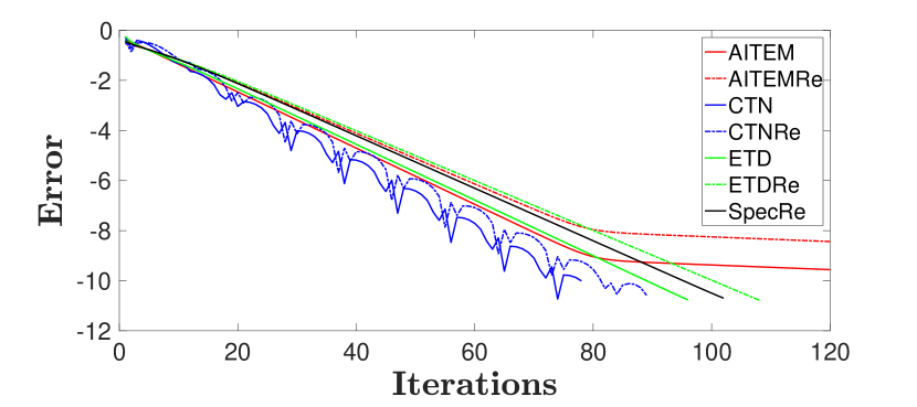
(a) $V(x)=0.1x^{2}$ , $\sigma=-1$

Scheme	$\Delta t$	$c$	$\tilde{n}$	$r$	Iterations
AITEM	.55	3	-	-	251
AITEMRe	.55	3	-	-	370
ACTN	.85	3	9	-	78
ACTNRe	.85	3	9	-	89
ETD	.16	-	-	-	96
ETDRe	.16	-	-	-	108
SpecRe	-	-	-	5.7	102
ETDV	.017	-	-	-	960

(b) $\mu=1.1848$

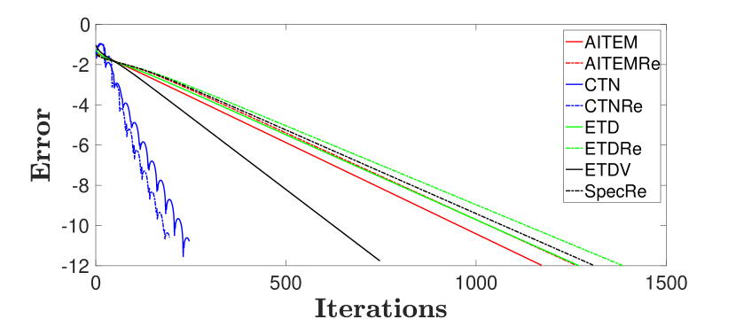
(c) $V(x)=0.01x^{4}+0.02x^{2}$ , $\sigma=-1$

Scheme	$\Delta t$	$c$	$\tilde{n}$	$r$	Iterations
AITEM	.052	4	-	-	1172
AITEMRe	.14	12	-	-	1260
ACTN	.3	5	23	-	246
ACTNRe	.35	6	20	-	194
ETD	.01	-	-	-	1270
ETDRe	.01	-	-	-	1385
SpecRe	-	-	-	94	1307
ETDV	.017	-	-	-	747

(d) $\mu=1.0393$

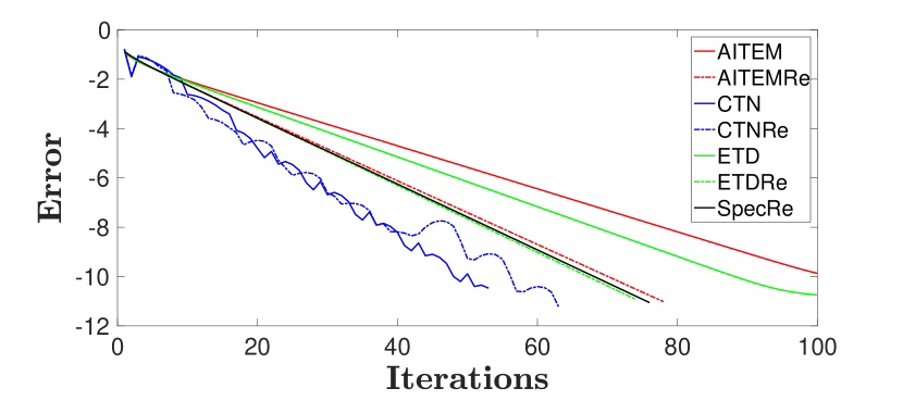
(e) $V(x)=0.1x^{2}$ , $\sigma=1$

Scheme	$\Delta t$	$c$	$\tilde{n}$	$r$	Iterations
AITEM	.85	6	-	-	252
AITEMRe	.83	6	-	-	78
ACTN	.9	4	23	-	53
ACTNRe	.9	4	20	-	63
ETD	.13	-	-	-	112
ETDRe	.12	-	-	-	74
SpecRe	-	-	-	7.5	76
ETDV	.017	-	-	-	695

(f) $\mu=-1.5955$

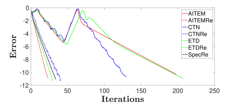
(g) $V(x)=\cos(x)$ , $\sigma=1$

Scheme	$\Delta t$	$c$	$\tilde{n}$	$r$	Iterations
AITEM	1.2	2	-	-	198
AITEMRe	1.4	3	-	-	23
ACTN	1.2	3	9	-	130
ACTNRe	1.1	4	4	-	41
ETD	.47	-	-	-	207
ETDRe	.4	-	-	-	30
SpecRe	-	-	-	2	34
ETDV	.016	-	-	-	3371

(h) $\mu=-2.6069$

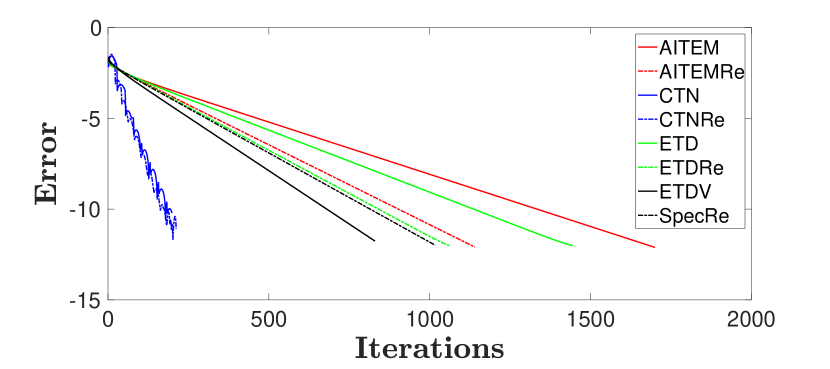
(i) $V(x)=0.01x^{4}+0.02x^{2}$ , $\sigma=1$

Scheme	$\Delta t$	$c$	$\tilde{n}$	$r$	Iterations
AITEM	.08	7	-	-	1700
AITEMRe	.09	8	-	-	1140
ACTN	.3	5	26	-	199
ACTNRe	.32	5	20	-	212
ETD	.01	-	-	-	1445
ETDRe	.4	-	-	-	1062
SpecRe	-	-	-	96	1017
ETDV	.017	-	-	-	830

(j) $\mu=-1.5795$

Figure 1: Evolution of the error, defined as the $L^{2}$ norm of the difference between successive iterates, as a function of the iteration index for different potentials $V(x)$, when seeking the ground state of the 1D NLS equation. The right set of tables indicates the values of the parameters selected and the corresponding number of iterations needed to reach the prescribed tolerance of $10^{-10}$.

There also does not appear to be any particular trend between the performance of a scheme and of its renormalized version; either one can outperform the other. That being said, Fig. 1(g) is particularly interesting. All of the renormalized methods converge to an unstable state centered at the origin –where the initial guess was also centered–. Nevertheless, the other methods converge to the stable, ground state, centered around $x=\pi$ i.e. around the minimum of the potential. Interestingly, notice how this “shift” takes place: while initially the method attempts to extremize by maintaining the waveform centered at the maximum, eventually, it cannot decrease the error below a certain threshold, being forced to seek a lower energy state by shifting the center of the coherent structure around $x=\pi$ (see the relevant trend after the 50th iteration), eventually decreasing the error in this new location below the desired tolerance.

The case reported in Fig. 2 bears some similarities to the above described scenario, as once again the state is initialized as located at the center, yet the double well nature of the potential does not favor such a localization at the maximum. Instead, the lowest energy state consists of a concentration of the atoms (or the optical power) in either the left or right well of the relevant potential. This symmetry-breaking is a feature well-known in the context of double-well potentials [rcg:BEC_book2]. The ETDV attempts for a while to extremize the free energy via localization at the center. Eventually, being unsuccessful, it is led to shift the wave mass to one of the two sides converging to the state shown in panel (g) of Fig. 3. This figure contains the ground state identified in all the cases of Figs. 1-2, rendering transparent that in case (d) and (g), the localization happens around $x\neq 0$.

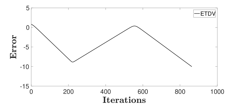
(a) $V=10x^{4}-20x^{2}$, $\sigma=1$

Scheme	$\Delta t$	$c$	$\tilde{n}$	$r$	Iterations
AITEM	-	-	-	-	DNC
AITEMRe	-	-	-	-	DNC
ACTN	-	-	-	-	DNC
ACTNRe	-	-	-	-	DNC
ETD	-	-	-	-	DNC
ETDRe	-	-	-	-	DNC
SpecRe	-	-	-	-	DNC
ETDV	.016	-	-	-	863

(b)

Figure 2: Similar to Fig. 1, but now for a double well potential. Only the ETDV is able to converge to the asymmetric ground state of this potential.

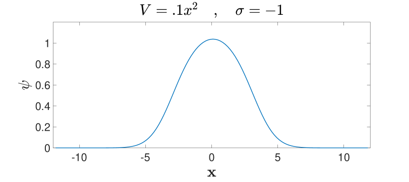
(a)

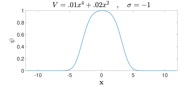
(b)

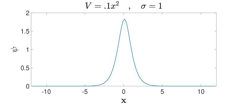
(c)

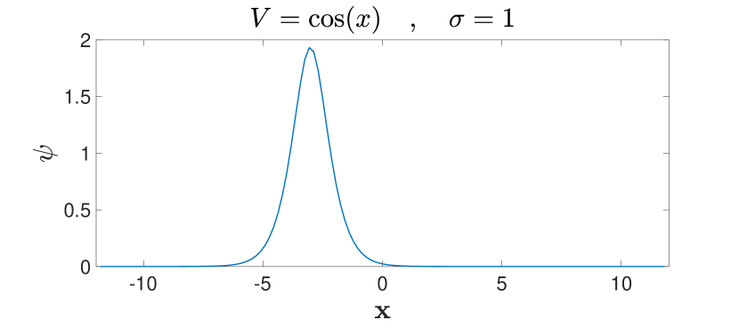
(d)

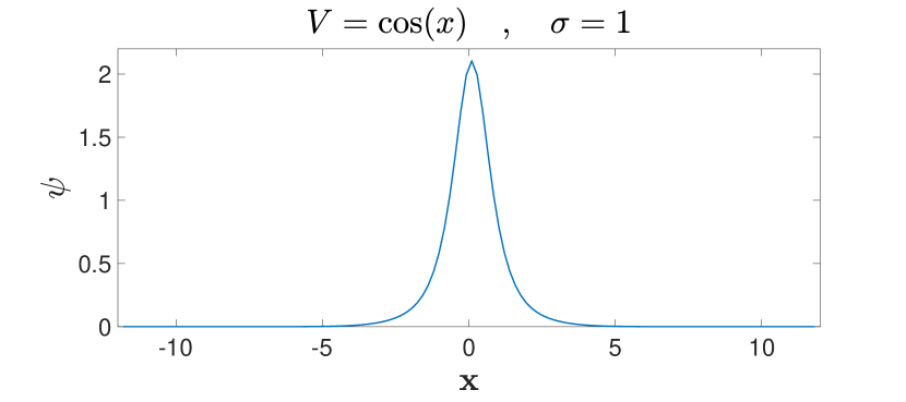
(e)

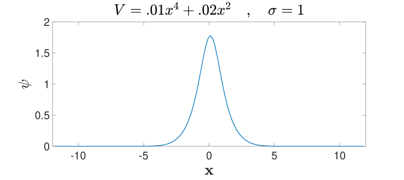
(f)

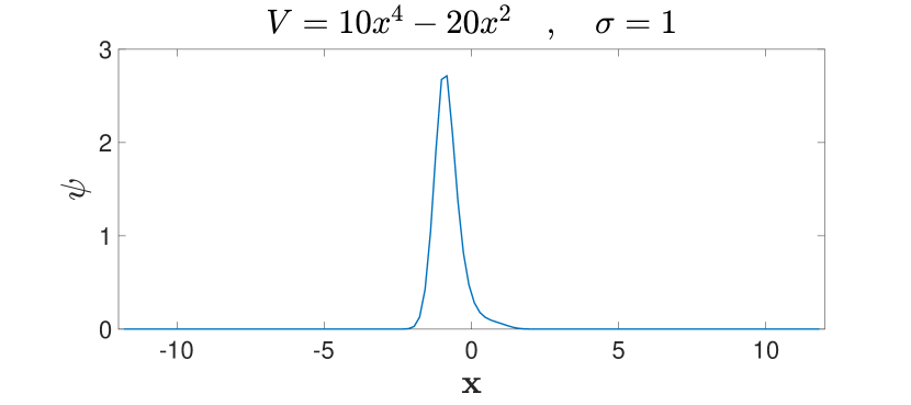
(g)

Figure 3: Corresponding steady states of the potentials analyzed in the previous two figures. Notice the $x\neq 0$ centering of cases (d) and (g).

B.  Ground States in 2D

In this section we focus on the 2D variant of the NLS equation, once again attempting to identify the ground state of the nonlinear elliptic problem. Fig. 4(a,b,c) is a defocusing NLS equation with quadratic potential. For the initial condition we use $\psi_{0}=Ae^{-(x^{2}+y^{2})}$, where $A$ is chosen so that the resulting power is $P=17$. Here, the ground single-hump state (whose linear limit is proportional to the initial guess) is rapidly converged upon. Fig. 4(d,e,f) is a focusing NLS equation with periodic potential and we use a similar initial condition except $A$ was chosen so that the chemical potential is $\mu=3.7$. In this case, all the schemes converge in a comparable number of iterations to a gap soliton solution of the problem.

As in the 1D case, the same general trends tend to hold. The continuous Nesterov methods seem to outperform the others, the ITEM schemes and ETD schemes seem to not have significant differences in their performance, and again there does not seem to be definitive preferentiability manifested between renormalized methods and their standard version.

C.  Excited States in 1D

Naturally, it is of substantial interest to go beyond the most fundamental states and seek excited states in the system. E.g. both in the atomic [GP, becbook1, becbook2, rcg:BEC_book2] and in the optical problem [kivshar], excited states such as dark solitons and multi-solitons in 1D and vortices and related structures (such as ring or planar dark solitons) in higher dimensions have been of particular interest.

In this section we combine ACTN with the so-called Squared Operator Method (SOM)[9] in order to capture such excited states. We quickly recap the basic idea: consider the gradient flow applied to some function $F$

$$\dot{u}=-F(u).$$

Naturally, this will only converge to local minima (in the case that $F$ is the gradient of some function) or, more generally, to a steady state having only eigenvalues with negative real part (if $F$ is not the gradient of some function). To extend this method to other steady states, one can instead consider the system

$$\dot{u}=-DF(u)F(u).$$

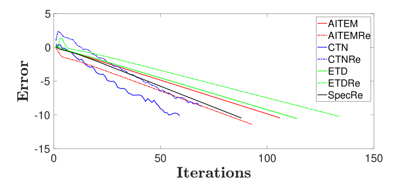
(a)

Scheme	$\Delta t$	$c$	$\tilde{n}$	$r$	Iterations
AITEM	1	3	-	-	106
AITEMRe	1.7	4	-	-	93
ACTN	1.1	2	5	-	59
ACTNRe	1.1	2	7	-	69
ETD	.3	-	-	-	114
ETDRe	.3	-	-	-	134
SpecRe	-	-	-	2.1	88

(b)

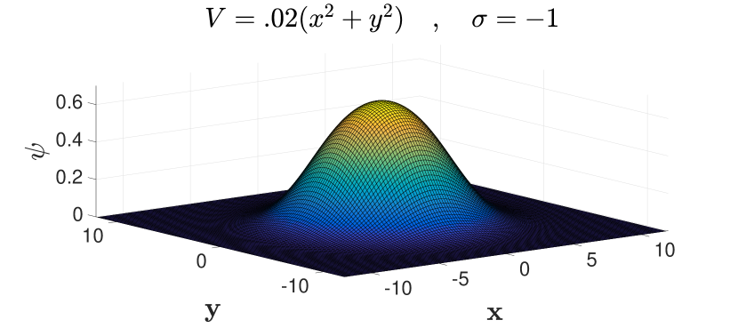
(c)

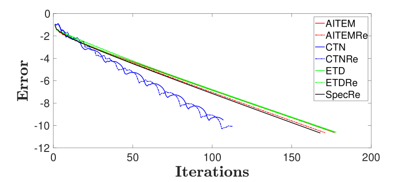
(d)

Scheme	$\Delta t$	$c$	$\tilde{n}$	$r$	Iterations
AITEM	1.1	3	-	-	177
AITEMRe	1.1	3	-	-	171
ACTN	1	2	5	-	107
ACTNRe	1	2	7	-	113
ETD	.31	-	-	-	178
ETDRe	.3	-	-	-	177
SpecRe	-	-	-	2.5	168

(e)

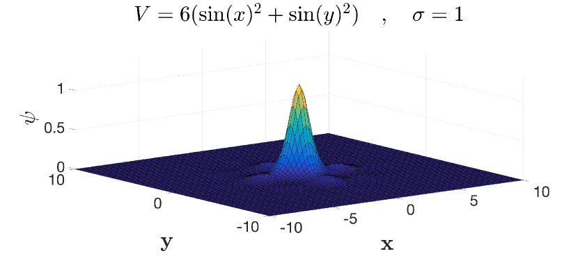
(f)

Figure 4: Two prototypical case examples in 2D. The top set of panels (a)-(c) displays the evolution of the error over the number of iterations, the parameters (and convergence iteration number) of the different methods, and the profile of the resulting solution for a parabolic trap in a defocusing 2D NLS with a Gaussian initial guess. Panels (d)-(f) report in similar format but now for a focusing 2D NLS with a periodic potential.

One quickly sees that every steady state of $F$ is a steady state of $DF(u)F(u)$ and, by taking the derivative of the RHS, one sees that every steady state of $F$ is stable in this new system. Hence, the SOM converges to every steady state of $F$ provided the initial condition is sufficiently close. Using CTN instead of the gradient flow, we get

$$\ddot{u}+\frac{3}{t}u+DF(u)F(u)=0.$$

It is this equation that we will study in what follows, and to which we will refer to as Squared (Operator) Continuous Time Nesterov (SCTN).

As an initial test, we seek families of stationary states of

$$\nabla^{2}\psi-0.1x^{2}\psi-\psi^{3}+\mu\psi=0$$

i.e., tackling the defocusing problem with a parabolic trap, in the spirit of earlier works such as [tristram, alfimov]. We apply the ACTN method to the SCTN equation, resulting in the iteration rcl M &= (c - ∇^2)^2
μ