Trapping and Escape in a Turbid Medium

Abstract

We investigate the absorption of diffusing molecules in a fluid-filled spherical beaker that contains many small reactive traps. The molecules are absorbed either by hitting a trap or by escaping via the beaker walls. In the physical situation where the number $N$ of traps is large and their radii $a$ are small compared to the beaker radius $R$, the fraction of molecules $E$ that escape to the beaker wall and the complementary fraction $T$ that eventually are absorbed by the traps depend only on the dimensionless parameter combination $\lambda=Na/R$. We compute $E$ and $T$ as a function of $\lambda$ for a spherical beaker and for beakers of other three-dimensional shapes. The asymptotic behavior is found to be universal: $1-E\sim\lambda$ for $\lambda\to 0$ and $E\sim\lambda^{-1/2}$ for $\lambda\to\infty$.

I Introduction

Consider a beaker filled with turbid medium—a fluid that contains many small reactive traps. We assume that the trap concentration is sufficiently low that interactions between traps can be ignored. Suppose that a molecule diffuses in the fluid and is absorbed whenever the molecule touches the surface of any of the traps or the wall of the beaker. Our basic goal is to compute the probability that the molecule is absorbed by the traps or by the beaker wall. In the latter case, the diffusing molecule can be viewed as escaping from the beaker. This type of system arises naturally in the absorption of photons in a multiple scattering medium, where extensive literature has discussed absorption and escape (see, e.g., BNHW87 ; CPW90 ; CMZ97 ; W98 ; W00 ; book:light ; cloak ).

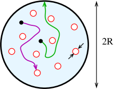
Figure 1: Sketch of a fluid-filled spherical beaker of radius $R$ that contains reactive traps of radius $a$. Shown are two diffusing molecules, one that escapes the beaker (green) and one that is absorbed by one of the traps (magenta).

For simplicity, we assume that the traps are identical spherical particles whose radii $a>0$ are small compared to the beaker radius. To simplify matters, we view the traps as immobile. This is a reasonable assumption if the traps are much larger than the diffusing molecules, and the treatment of the general case is essentially identical as we will discuss. We assume that the number of traps is sufficiently large that fluctuations in their local density can be ignored. In this limit, it is generally possible to replace the discrete traps by an effective average trapping medium. The dynamics of the molecules can then be described by a reaction-diffusion equation, for which explicit solutions can be obtained by standard methods. The converse situation where the beaker contains a few traps or the trapping efficiency of each trap is distributed is challenging, because the trapping probability depends in detail on the trap positions, and the effective-medium approach no longer applies.

Eventually all the molecules are absorbed by either the traps or by the beaker wall. What is the fraction $E$ that reach the beaker wall? What is the fraction $T$ that get absorbed by the traps? Our goal is to calculate these escape and trapping probabilities, $E$ and $T$ respectively, for simple geometries. We will first study the case of a spherical beaker of radius $R$ in three dimensions and then generalize to arbitrary spatial dimensions $d$ and to beakers of other simple shapes, such as a parallelepiped and a cylinder.

We begin, in Sec. II by writing the dynamical equation and governs the escape and trapping probabilities and develop an equivalent time-independent description for these probabilities. Although the molecule density evolves with time, it is possible to recast the infinite-time escape and trapping probabilities as a simpler time-independent problem. In Sec. III, we use this perspective to solve the idealized situation of a single trap of radius $a$ at the center of a beaker of radius $R$. We also extend this solution to a non-concentric geometry in two dimensions.

In Sec. IV, we treat our primary example of the escape of a diffusing molecule from a spherical beaker that contains $N\gg 1$ traps. In principle, we have to solve the diffusion equation in the available volume—the region exterior to the traps and interior to the beaker—and then compute the time integrated fluxes to the traps and to the beaker walls. A full solution to this formidable problem is not feasible, and instead we apply the powerful reaction-rate approach (RRA) smol ; chandra ; R01 ; book ; ovchin ; B93 ; gleb . Here we replace the discrete traps by an spatially uniform effective trapping medium, leading to a problem that is readily soluble by standard methods.

Generically, one might anticipate that the exit probability should depend on two dimensionless parameters: $N$ and $a/R$. We shall show, however, that the exit probability $E(N,a/R)$ depends only on a single parameter, which is the product of $N$ and $a/R$:

$$\lambda=N\,\frac{a}{R}\,.$$ (1)

If one knew in advance that the behavior is determined by a single parameter, one might anticipate that it might be $N(a/R)^{3}$, the ratio of the trap volume to the system volume, or perhaps $N(a/R)^{2}$, the ratio of the total surface of the traps to the total exit area. Thus the dependence on a single parameter, specifically on $\lambda=Na/R$, could be puzzling at first sight; we shall show, however, that this dependence follows naturally from the structure of the RRA.

In Sec. V, we obtain the explicit solution for the exit probability $E(\lambda)$ for a spherical beaker in three dimensions by the RRA. The exit probability is given by the following compact formula

$$E(\lambda)=3\,\frac{\coth(\sqrt{3\lambda})}{\sqrt{3\lambda}}-\frac{1}{\lambda}$$ (2)

The form of the exit probability is sensitive to the shape of the beaker, but the limiting behaviors

$$\begin{split}T&=1-E\sim\lambda\qquad\text{as\ }\lambda\to 0,\\ E&\sim\lambda^{-1/2}\qquad\qquad\text{as\ }\lambda\to\infty,\end{split}$$ (3)

are universal, they generally apply for non-pathological beaker shapes; only the amplitudes of these scaling laws are shape dependent. It bears emphasizing that the volume fraction occupied by the traps $\varphi=N(a/R)^{3}$ is generally small in realistic systems. However, since $\lambda=N^{2/3}\,\varphi^{1/3}$, the parameter $\lambda$ does not have to be small, even for $\varphi\ll 1$. Thus a dilute system of traps can be strongly absorbing. A similar situation arises in the case of small absorbing receptors on the surface of an otherwise reflecting sphere BP77 . This system can have an absorption coefficient that is nearly the same as that of a perfectly absorbing sphere for a small receptor density.

II Time-Independent Formalism

We seek the exit probability $E({\bf r}_{0})$ for a molecule to be absorbed at the surface of the beaker, given that the molecule starts at ${\bf r}_{0}$. There is also the complementary trapping probability $T({\bf r}_{0})$ for a molecule to be absorbed at the surface of one of the traps. To determine the exit probability, we should solve the diffusion equation

$$\frac{\partial P}{\partial t}=D\nabla^{2}P$$ (4)

for the molecular density $\rho({\bf r},t)$, with the initial condition $\rho({\bf r},t\!=\!0)=\delta({\bf r}-{\bf r}_{0})$, and with absorbing boundary conditions $\rho=0$ on the surfaces of all traps and on the beaker wall. The exit probability $E({\bf r}_{0})$ equals the local flux $-D\nabla\rho$, integrated over the beaker surface and over all time. If we assume that the molecules are uniformly distributed throughout the beaker, the exit probability, averaged over the initial molecular positions, is

$$E=\frac{\int d{\bf r}_{0}\,E({\bf r}_{0})}{\int d{\bf r}_{0}}\,,$$ (5)

where the integrals extend over the allowed spatial region of the molecules.

Because the time does not appear in $E({\bf r}_{0})$, the problem can be recast into a time-independent form by integrating Eq. (4) over all time. By this approach, one finds that $E({\bf r}_{0})$ satisfies the backward Kolmogorov equation R01 ; book

$$\nabla_{0}^{2}E=0,$$ (6)

where the subscript $0$ indicates the the derivatives in the Laplacian refer to the initial coordinates of the molecule. This backward equation should be solved subject to the boundary conditions

$$E|_{\rm traps}=0,\qquad\qquad E|_{\rm wall}=1\,.$$

The first condition merely states that a molecule starting on a trap surface cannot reach the beaker wall, while the second states a molecule starting on the beaker wall necessarily exits. The exit probability thus satisfies the Laplace equation for the electrostatic potential in the same geometry, with the traps and the beaker wall substituted by conductors. We may now utilize well-known results for the corresponding electrostatic system S ; LL to determine the exit probability.

III Single Trap

We first determine the exit probability $E$ for a single spherical trap of radius $a$ centered inside a spherical beaker of radius $R$. For ease of notation, we define $E_{-}(r)$ be the probability that a molecule that starts at distance $r$ from the origin will be absorbed by the inner sphere (the trap); thus $E_{-}(r)$ corresponds to the trapping probability defined above. Similarly, let $E_{+}(r)$ be the probability to first reach the outer sphere—the escape probability defined previously. As discussed above, $E_{+}$ and $E_{-}$ satisfy the Laplace equation

$$\nabla^{2}E_{\pm}(r)=0\,,$$ (7)

subject to the boundary conditions

$$E_{+}(a)=0,\qquad E_{+}(R)=1,$$

$$E_{-}(a)=1,\qquad E_{-}(R)=0.$$

By spherical symmetry, we only need to solve the radial part of the Laplace equation (7) subject to these boundary conditions, from which the exit probability is R01 :

$$E_{+}(r)=\begin{cases}{\displaystyle\frac{1-(a/r)^{d-2}}{1-\lambda^{d-2}}}&\quad d\neq 2,\\ \\ {\displaystyle\frac{\ln(r/a)}{\ln(1/\lambda)}}&\quad d=2,\end{cases}$$ (8)

with $\lambda=a/R$. Since there is only a single “trap”, the quantity $\lambda$ defined here is equivalent to that given in Eq. (1). The trapping probability is complementary quantity: $E_{-}(r)=1-E_{+}(r)$.

To compute to exit probability averaged over all molecules, we assume that they are uniformly distributed in the annulus $a<r<R$, so that the density in the range $(r,r+dr)$ is proportional to $r^{d-1}dr$. The total exit probability is then

$$E=\int_{a}^{R}dr\,r^{d-1}\,E_{+}(r)\Bigg{/}\left(\int_{a}^{R}dr\,r^{d-1}\right)\,.$$ (9)

Using (8)–(9) gives, in three dimensions,

$$E=\frac{1+\lambda/2}{1+\lambda+\lambda^{2}}\,,\qquad\lambda=\frac{a}{R}~{}.$$ (10a)

Notice that the fraction of molecules that exit from the beaker decreases from 1 to 1/2 as $$\lambda \lambda\to 0 \lambda\to 1$$ increases from 0 to 1. When , the trap at the origin has negligible size so that nearly all molecules will escape the beaker. Conversely, as , the physical region becomes an infinitesimally thin annulus, which can be approximated as a slab. In this case, the molecule is equally likely to escape via either boundary. In two dimensions, the solution to the Laplace equation (7) is again straightforward to obtain and the corresponding result for the exit probability is

$$E=\frac{1}{1-\lambda^{2}}-\frac{1}{2\ln(1/\lambda)}~{}.$$ (10b)

This expression has the same limiting behaviors as in the case of $d\neq 2$.

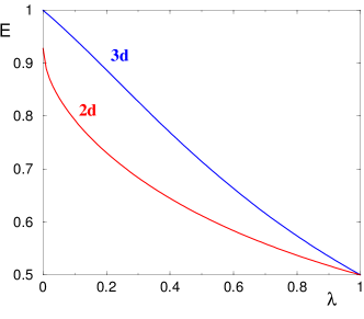
Figure 2: The exit probability $E(\lambda)$, with $\lambda=R_{-}/R_{+}$ in three and two dimensions (Eqs. (10a) and (10b) for a single trap inside a beaker when the trap and beaker are concentric spheres of radii $R_{-}$ and $R_{+}$.

We can also extend the above approach to a trap that is located non-symmetrically within a spherical beaker. In this case, the Laplace equation $\nabla^{2}E({\bf r})=0$ does not have a compact closed-form solution in three dimensions S . In two dimensions, however, the corresponding solution for $E(x,y)$ is known LL . Suppose that the beaker is centered at the origin while the trap is centered at $(c,0)$ (with $c<R-a$ to ensure that the trap is entirely inside the beaker). In the corresponding electrostatic problem, the potential between the conductors is identical to the potential induced by two equal and opposite point charges that are located at $(c+d_{1},0)$ and $(d_{2},0)$, with

$$d_{1}(d_{2}-c)=a^{2},\quad d_{2}(c-d_{1})=R^{2}\,.$$

We now let

$$r_{1}=\sqrt{(x-c-d_{1})^{2}+y^{2}}\,,\quad r_{2}=\sqrt{(x-d_{1})^{2}+y^{2}}$$

be the distances between each charge and the diffusing molecule, with the molecule initially at $(x,y)\in\mathcal{R}$, with

$$\mathcal{R}=\{(x,y)|x^{2}+y^{2}<R^{2},~{}~{}(x-c)^{2}+y^{2}>a^{2}\}$$

the region between the conductors. The probability that a molecule that starts at $(x,y)$ is absorbed by the beaker wall is

$$E(x,y)={\ln\left(\frac{r_{2}}{r_{1}}\frac{d_{1}}{a}\right)}\Big{/}{\ln\left(\frac{d_{1}d_{2}}{aR}\right)}~{}.$$ (11)

The exit probability is the spatial average of $E(x,y)$ over the region $\mathcal{R}$:

$$E=\frac{1}{\pi(R^{2}-a^{2})}\int\!\!\!\int_{\mathcal{R}}dxdy\,E(x,y)\,.$$ (12)

This double integral does not seem to be expressible through known functions, however. Thus for the simplest setting of a single circular trap inside a circular beaker, the exit probability has a closed form only when these two objects are concentric.

IV Reaction-Rate Approach

The Smoluchowski reaction-rate approach (RRA) is an effective-medium approximation that replaces the complicated influences of each individual trap by their average influence (see, e.g., R01 ; book ; smol ; chandra ; ovchin ; B93 ; gleb ). In this approach, the diffusion equation (4) is replaced by the reaction-diffusion equation

$$\frac{\partial\rho}{\partial t}=D\nabla^{2}\rho-K\rho\,,$$ (13)

where $K$ is the reaction rate that accounts for the average absorption rate of diffusing molecules by the traps. For identical spherical traps, the reaction rate is R01 ; book ; smol ; chandra ; ovchin ; B93 ; gleb )

$$K=4\pi Da\,n\,,$$ (14a)

where $$n=N/V N V K$$ (with the number of traps and the beaker volume) is the trap density. This expression for is asymptotically exact when the volume fraction of the traps is small, so that their interactions can be neglected. The RRA can be generalized in a straightforward way to cases where the traps are mobile and where the size of the molecules cannot be ignored.

It is easiest to compute the reaction rate via the electrostatic analogy (apparently first noticed in the classical paper BP77 ; see B93 ; book for reviews). This approach gives

$$K=4\pi DnC\,,$$ (14b)

where $C$ is the electrical capacitance of the trap (assuming that it is a perfect conductor of the same shape). As examples, a sphere of radius $a$ has capacitance $C=a$, so that (14b) reduces to (14a); a disk of radius $a$ has capacitance $2a/\pi$, leading to $K=8Dan$. The electrical capacitance of ellipsoids is also known. For instance, for oblate spheroids with semi-axes $a=a\leq b$ the reaction rate is

$$K=4\pi Dn\,\frac{\sqrt{a^{2}-b^{2}}}{\cos^{-1}(b/a)}\,.$$

In the following we treat spherical traps and use (14a); arbitrary geometries can be obtained by straightforward generalization.

Within the RRA, we need to solve the reaction-diffusion equation with an absorbing boundary condition at the beaker wall

$$\rho\big{|}_{\rm wall}=0\,,$$ (15)

for a spatially uniform initial condition $\rho(\mathbf{r},t=0)=1$. Since the molecular flux to the wall is $-D\nabla\rho$, the total number of molecules that exit the beaker is

$$-\int_{0}^{\infty}dt\int dS\,{\bf n}\cdot D\nabla\rho\,,$$

where the second integral is over the beaker wall and ${\bf n}$ is the unit normal to the wall. Dividing by the total initial number of molecules $V$ gives the exit probability

$$E=\frac{1}{V}\int_{0}^{\infty}dt\int dS\,{\bf n}\cdot D\nabla\rho\,.$$ (16)

V Trapping and Escape Probabilities

We now compute the escape and trapping probabilities for: (i) a spherical beaker in three directions, (ii) a spherical beaker in general dimensions, and finally (iii) other simple beaker shapes in three dimensions. Throughout, we consider the traps to be identical small spheres; however, our results can be extended to traps of other shapes if the electrostatic capacitance of this shape is known.

V.1 Three dimensions

For spherical traps, the reaction rate is given by (14a). When the beaker is a ball of radius $R$, the surface integral in (16) is readily performed and the exit probability is

$$E=\frac{3D}{R}\int_{0}^{\infty}dt\left[-\frac{\partial\rho}{\partial r}\right]\Bigg{|}_{r=R}~{}.$$ (17)

To compute this integral, we must solve the reaction-diffusion equation (13). This solution (Appendix A) gives the concentration $\rho$ as the Fourier series

$$\rho(r,t)=\frac{2}{r}\sum_{n=1}^{\infty}\frac{(-1)^{n+1}}{\pi n}\,e^{-(n^{2}\pi^{2}+3\lambda)t}\,\,\sin(n\pi r)\,.$$ (18)

Substituting this expression in (17) and performing the integral, the exit probability is

$$E=\sum_{n=1}^{\infty}\frac{6}{n^{2}\pi^{2}+3\lambda}=3\,\frac{\coth(\sqrt{3\lambda})}{\sqrt{3\lambda}}-\frac{1}{\lambda}~{}.$$ (19)

The second equality has been obtained by standard residue calculus methods.

The limiting behaviors of Eq. (19) are instructive. As $\lambda\to 0$, we obtain

$$E =1-\frac{1}{5}\,\lambda+\frac{2}{35}\,\lambda^{2}-\frac{3}{175}\,\lambda^{3}+\frac{2}{385}\,\lambda^{4}-\ldots$$ (20a)

while in the opposite $$\lambda\to\infty$$ limit

$$E\simeq\sqrt{\frac{3}{\lambda}}-\frac{1}{\lambda}~{}.$$ (20b)

The latter approximation is almost indistinguishable from the exact solution (19) for $\lambda\gtrsim 3$ (see Fig. 3), because the next correction term in (20b) is of the order of $e^{-\sqrt{12\lambda}}$. As we shall see, these two limiting behaviors of $T\sim\lambda$ for $\lambda\to 0$ and $E\sim\lambda^{-1/2}$ for $\lambda\to\infty$ arise quite generally.

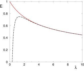
Figure 3: The exit probability $E(\lambda)$, with $\lambda$ given by (1) when the number of traps is large and the beaker is a ball of radius $R$. The solid curve is the exact result Eq. (19), while the dashed curve is the approximation, Eq. (20b).

V.2 General dimensions

For general spatial dimensions, we must solve the $d$-dimensional reaction-diffusion (13). Using spherical symmetry, we assume that the initial condition is a normalized spherical shell of probability at $r=r_{0}$:

$$\rho(r,t\!=\!0)=\frac{\delta(r-r_{0})}{\Omega_{d}r_{0}^{d-1}}~{},$$

where $\Omega_{d}$ is the surface area of a $d$-dimensional unit sphere. We now Laplace transform (13) and re-express the radius in dimensionless units $x=r\sqrt{s/D}$, after which the reaction-diffusion equation (13) becomes

$$\tilde{\rho}\,^{\prime\prime}+\frac{d-1}{x}\,\tilde{\rho}\,^{\prime}-\Big{(}1+\frac{\lambda}{s}\Big{)}\tilde{\rho}=-\frac{s^{(d-2)/2}}{D^{d/2}}\frac{\delta(x-x_{0})}{\Omega_{d}x_{0}^{d-1}}~{}.$$ (21)

Here the tilde denotes the Laplace transform, and the prime denotes differentiation with respect to $x$. This equation should be solved subject to the boundary condition $\rho(R,t)=0$.

From the solution to Eq. (21) (see Appendix B), the probability $E(r_{0})$ that a diffusing molecule that starts at $r_{0}$ ultimately escapes to the beaker wall is given by

$$E(r_{0})=\left(\frac{r_{0}}{R}\right)^{\nu}\frac{I_{\nu}(\mu r_{0})}{I_{\nu}(\mu R)}~{}.$$ (22)

Here $I_{\nu}$ and $K_{\nu}$ are the modified Bessel functions of order $\nu$, with $\nu=(2\!-\!d)/2$, and $\mu=\sqrt{1\!+\!\lambda/s}$.

A more meaningful measure of the trapping efficiency of the system is the escape probability when the fluid initially contains a uniform density of diffusing molecules. Here we need to integrate (22) over all radii and also modify (22) for the initial condition of a uniform density in the entire beaker, rather than a spherically symmetric density shell at radius $r_{0}$. For the latter, we merely need to multiply the result of integrating (22) over all radii by the factor ${d}/{R}$ to account for the difference is the normalizations between a uniform density within a sphere and on a spherical surface.

For the spatial integration, we make use of the identity

$$\frac{d}{dz}\big{[}z^{\nu}I_{\nu}(z)\big{]}=z^{\nu}I_{\nu-1}(z)\,,$$

as well as $I_{\nu}=I_{-\nu}$ to write

$$E =\frac{d}{R}\int_{0}^{R}\!r^{d-1}\,E(r)\,dr$$

$$=\frac{d}{R}\int_{0}^{R}\!r^{d-1+\nu}\,\,\frac{I_{\nu}(\mu r)}{I_{\nu}(\mu R)}\,dr$$

$$=\frac{d}{R}\int_{0}^{R}\!r^{d/2}\,\,\frac{I_{(d-2)/2}(\mu r)}{I_{(d-2)/2}(\mu R)}\,dr$$

$$=\frac{d}{\mu R}\,\,\frac{I_{d/2}(\mu R)}{I_{(d-2)/2}(\mu R)}~{}.$$ (23)

In three dimensions, the above expression reduces to that given in (19). From (V.2), the exit probability has the same asymptotic behaviors (3) in all dimensions $d>2$.

VI Discussion

We studied the trapping characteristics of diffusing molecules that are absorbed whenever they either reach the boundary of a finite fluid-filled beaker or touch traps within the fluid. The solution for a single trap is simple for the example of a spherical trap at the center of a spherical beaker. It is impractical, however, to generalize this analytical approach for more than a single trap because it involves solving the diffusion equation subject to absorbing boundary conditions on the surface of all traps and the surface of the beaker. However, the problem greatly simplifies when there are many traps. In this limit, we can replace the traps by an effective and uniformly absorbing medium—the reaction rate approximation (RRA). We showed how to compute the fraction of molecules that escape the domain for the situation where the total number of traps is large. Remarkably, this escape probability depends only on a single parameter $\lambda$, the product of the total number of traps and the ratio of the characteristic size of the trap to the characteristic size of the domain. Our general results is that the exit probability from the beaker, $E$, exhibits universal asymptotic behaviors (3) in all dimensions greater than two.

While our model describes the absorption of diffusing molecules in a beaker that contains a reactive fluid, there are other other potential scenarios. For example, the domain could be a cell and the diffusing molecules may exit the cell membrane, or may be absorbed by traps within the cell and thereby perform some biologically useful function. Here, exit may be treated as a loss and one would like to estimate the magnitude of the loss. In realistic systems, the parameter $\lambda$ is usually large, so our results can be interpreted as the generic claim that this loss, viz., the fraction of molecules exiting through the cell membrane, universally scales as $A/\sqrt{\lambda}$ when $\lambda\gg 1$. Only the amplitude $A$ depends on the shape of the cell and on the shape of the traps.

Within the RRA, we determined the exit and trapping probabilities without needing to solve the underlying reaction-diffusion equation. In addition to simplifying the calculations, the RRA provides additional insights that would be very difficult to obtain by direct means. For example, for a cylindrical beaker of radius $R$ and height $H$, the exit probability could, in principle, depend on three dimensionless parameters: $N$, $a/R$, and $R/H$. The RRA predicts that for very tall cylinders ($R\ll H$), the exit probability again actually depends on the single parameter $\lambda=Na/H$. It is worth noting that within the RRA formalism it also is straightforward to account for diffusing traps as well as a non-zero radii for both the traps and the molecules. All that is needed is to amend the parameter $\lambda$ from $Na/R$ to

$$\lambda=N\,\frac{a_{m}+a_{t}}{R}\,\frac{D_{m}+D_{t}}{D_{m}}\,,$$ (24)

where the subscripts $m$ and $t$ refer to the molecules and the traps, respectively.

We thank Sergei Rudchenko, Nagendra K. Panduranga and Kirill Korolev for helpful discussions. This work was partly supported by the National Science Foundation under grant No. DMR-1608211.

Appendix A Concentration in Three Dimensions

To solve the reaction-diffusion equation (13) in three dimensions, we use a simplification that transforms the radial Laplacian that operates on the quantity $u(r)/r$ to a one-dimensional Laplacian:

$$\frac{1}{r^{2}}\,\frac{\partial}{\partial r}\left(r^{2}\,\frac{\partial}{\partial r}\right)\frac{u}{r}=\frac{1}{r}\,\frac{\partial^{2}u}{\partial r^{2}}~{}.$$ (25)

This identity suggests that we work with $u=\rho\,r$, after which the reaction-diffusion equation, with $K$ given by (14a), becomes

$$\frac{\partial u}{\partial t}=D\left(\frac{\partial^{2}}{\partial r^{2}}-\frac{3Na}{R^{3}}\right)u\,.$$ (26)

It is useful to now introduce the dimensionless variables

$$\overline{r}=\frac{r}{R}\,,\qquad\overline{t}=\frac{Dt}{R^{2}}~{},$$ (27)

and then drop the overbars to simplify notation in the following. Equation (26) becomes

$$\frac{\partial u}{\partial t}=\frac{\partial^{2}u}{\partial r^{2}}-3\lambda u,\qquad\lambda=N\,\frac{a}{R}~{}.$$ (28)

We want to solve (28) subject to the condition of a uniform initial density

$$u|_{t=0}=r\,,$$ (29a)

an absorbing boundary condition at the beaker wall

$$u|_{r=1}=0\,,$$ (29b)

and the condition

$$u|_{r=0}=0\,$$ (29c)

that ensures that $\rho=u/r$ is well-defined in the origin. The exit probability (17) now becomes

$$E=3\int_{0}^{\infty}dt\left[-\frac{\partial u}{\partial r}\right]\Bigg{|}_{r=1}$$ (30)

We use Fourier analysis (see, e.g., DMK ) to solve Eq. (28) subject to (29). Here it is useful to extend the domain of $u(r,t)$ from $[0,1]$ to $[-1,1]$. For convenience we also extend $u$ to be odd (i.e., $u(-r)=-u(r)$), so that the boundary condition (29c) manifestly holds. Then the Fourier expansion of $u(r,t)$ contains only sine terms:

$$u(r,t)=\sum_{n=1}^{\infty}F_{n}(t)\,\sin(n\pi r)\,.$$ (31)

From the initial condition (29a) we obtain

$$F_{n}(0)=2\int_{0}^{1}dr\,r\,\sin(n\pi r)=2\,\frac{(-1)^{n+1}}{\pi n}~{}.$$

Substituting (31) into (28) gives the differential equation for the amplitudes

$$\frac{dF_{n}}{dt}=-(n^{2}\pi^{2}+3\lambda)\,F_{n}\,.$$

Solving this equation, the concentration $\rho(r,t)$ may be written as the infinite series in Eq. (18).

Appendix B General Dimensions

The Laplace transform of the reaction-diffusion equation Eq. (21) is

$$\tilde{\rho}^{\prime\prime}+\frac{d-1}{x}\,\tilde{\rho}^{\prime}-\Big{(}1+\frac{\lambda}{s}\Big{)}\tilde{\rho}=-\frac{s^{(d-2)/2}}{D^{d/2}}\frac{\delta(x-x_{0})}{\Omega_{d}x_{0}^{d-1}}~{},$$ (32)

where $x=r\sqrt{s/D}$ is the scaled coordinate, and $x$ is in the range $(0,X)$, with $X=R\sqrt{s/D}$. This equation should be solved subject to the absorbing boundary condition at $x=X$. The left-hand side of (32) is a Bessel differential equation that we solve separately for $x<x_{0}$ and $x>x_{0}$, and then patch together these two solutions by the standard joining conditions for Green’s functions. In each subdomain $x<x_{0}$ and $x>x_{0}$, the elemental solutions have the form

$$\begin{split}\rho_{<}&=Ax^{\nu}I_{\nu}(\mu x)\,,\\ \rho_{>}&=Bx^{\nu}I_{\nu}(\mu x)+Cx^{\nu}K_{\nu}(\mu x)\,.\end{split}$$ (33)

Here $I_{\nu}$ and $K_{\nu}$ are the modified Bessel functions of order $\nu$, with $\nu=(2\!-\!d)/2$, and $\mu=\sqrt{1\!+\!\lambda/s}$. The subscripts $<$ and $>$ denote the solution in the regions $x<x_{0}$ and $x>x_{0}$. The interior solution does not contain the function $K_{\nu}$ because $K_{\nu}$ diverges at the origin. Invoking the absorbing boundary condition $\rho=0$ at $x=X$, as well as the continuity of the Green’s function at $r=r_{0}$, the solution (33) can be expressed in a form that is manifestly continuous and vanishes at $x=X$:

$$\begin{split}\rho_{<}&=Ax^{\nu}I_{\nu}(\mu x)\big{[}I_{\nu}(\mu x_{0})K_{\nu}(\mu X)-I_{\nu}(\mu X)K_{\nu}(\mu x_{0})\big{]}\,,\\ \rho_{>}&=Ax^{\nu}I_{\nu}(\mu x_{0})\big{[}I_{\nu}(\mu x)K_{\nu}(\mu X)-I_{\nu}(\mu X)K_{\nu}(\mu x)\big{]}\,.\end{split}$$

The constant $A$ is determined by the joining condition

$$D(\rho_{>}^{\prime}-\rho_{<}^{\prime})\Big{|}_{x_{0}}=-\frac{s^{(d-2)/2}\,\delta(x-x_{0})}{D^{d/2}\,\Omega_{d}\,\,x_{0}^{d-1}}~{}.$$

For differentiating the Green’s function, we use

$$I_{\nu}^{\prime}=\frac{\nu}{x}I_{\nu}+I_{\nu-1}\quad\text{and}\quad K_{\nu}^{\prime}=\frac{\nu}{x}K_{\nu}-K_{\nu-1}\,,$$

while for $\rho_{>}^{\prime}-\rho_{<}^{\prime}$, we use the Wronskian relation

$$x_{0}\big{[}I_{\nu-1}(x_{0})K_{\nu}(x_{0})+K_{\nu-1}(x_{0})I_{\nu}(x_{0})\big{]}=1.$$

With these identities and performing some tedious but straightforward algebra, the amplitude of the Green’s function is given by

$$A=\frac{(s/x_{0})^{(d-2)/2}}{D^{1+d/2}\,\Omega_{d}\,I_{\nu}(\mu X)}\,.$$

Finally, we compute the flux $-D\rho^{\prime}$ to the outer boundary, integrate over the surface of the sphere, and then take the $s\to 0$ limit of the Laplace transform to obtain the probability $E(r_{0})$ that a diffusing molecule that starts at $x_{0}$ ultimately escapes to the beaker wall. This is Eq. (22).

Appendix C Other Geometries

Here we solve (13) and compute the exit probability for two additional cases.

C.1 Parallelepiped

Consider the parallelepiped of size $L_{1}\times L_{2}\times L_{3}$. The reaction-diffusion equation is

$$\frac{\partial\rho}{\partial t}=D\left(\nabla^{2}\rho-\frac{4\pi aN}{L_{1}\,L_{2}\,L_{3}}\,\rho\right)~{}.$$ (34)

We seek a solution in the form of a Fourier sine series

$$\rho(r,t)=\sum_{n_{1},n_{2},n_{3}\geq 1}F_{\bf n}(t)\prod_{j=1}^{3}\sin\left(n_{j}\,\pi\frac{x_{j}}{L_{j}}\right)~{},$$ (35)

which ensures that the absorbing boundary condition (15) is automatically satisfied on the walls $x_{j}=0,L_{j}$. Substituting (35) into (34) and solving for $F_{\bf n}(t)$ gives

$$F_{\bf n}(t)=F_{\bf n}(0)\,\exp[-\pi^{2}\Lambda({\bf n})Dt]\,,$$

where we use the shorthand notation

$$\Lambda({\bf n})=\left(\frac{n_{1}}{L_{1}}\right)^{2}+\left(\frac{n_{2}}{L_{2}}\right)^{2}+\left(\frac{n_{3}}{L_{3}}\right)^{2}+\frac{4}{\pi}\,\frac{aN}{L_{1}\,L_{2}\,L_{3}}\,.$$

For the spatially uniform initial condition we find that $F_{\bf n}(0)=0$ if at least one index $n_{j}$ is even; when all $n_{j}$’s are odd, we have

$$F_{\bf n}(0)=\frac{8^{2}}{\pi^{3}}\,\frac{1}{n_{1}\,n_{2}\,n_{3}}\,.$$

After some straightforward calculations, the exit probability is

$$E=\frac{8^{3}}{\pi^{6}}\sum_{\bf n}\left[\frac{1}{L_{1}^{2}\,n_{2}^{2}\,n_{3}^{2}}+\frac{1}{L_{2}^{2}\,n_{3}^{2}\,n_{1}^{2}}+\frac{1}{L_{3}^{2}\,n_{1}^{2}\,n_{2}^{2}}\right]\frac{1}{\Lambda({\bf n})}~{}.$$

Here and below the $\sum_{\bf n}$ runs over $n_{1},n_{2},n_{3}$ which are all positive and odd.

Let us consider two examples in more detail. For the cube with $L_{1}=L_{2}=L_{3}=L$, we obtain

$$E=\frac{8^{3}}{\pi^{6}}\sum_{\bf n}\frac{1}{n_{1}^{2}\,n_{2}^{2}\,n_{3}^{2}}\,\,\frac{{\bf n}^{2}}{{\bf n}^{2}+\lambda}\,,$$ (36)

where we use the shorthand ${\bf n}^{2}=n_{1}^{2}+n_{2}^{2}+n_{3}^{2}$ with $\lambda=4aN/\pi L$ note . Using (36) and the identity knuth

$$\sum_{n~{}\text{odd}}\frac{1}{n^{2}}=\frac{\pi^{2}}{8}\,,$$ (37)

we determine the trapping probability

$$T=\frac{8^{3}}{\pi^{6}}\sum_{\bf n}\frac{1}{n_{1}^{2}\,n_{2}^{2}\,n_{3}^{2}}\,\,\frac{\lambda}{{\bf n}^{2}+\lambda}~{}.$$ (38)

The small $\lambda$ expansion of this trapping probability is

$$T=A_{1}\lambda-A_{2}\lambda^{2}+A_{3}\lambda^{3}-A_{4}\lambda^{4}+\ldots\,,$$ (39)

where

$$A_{p}=\frac{8^{3}}{\pi^{6}}\sum_{\bf n}\frac{1}{n_{1}^{2}\,n_{2}^{2}\,n_{3}^{2}}\,\,\frac{1}{(n_{1}^{2}+n_{2}^{2}+n_{3}^{2})^{p}}~{}.$$

To determine the large-$\lambda$ behavior, we use symmetry and re-write (36) as

$$E=3\,\frac{8^{3}}{\pi^{6}}\sum_{n_{2},\,n_{3}}\frac{1}{n_{2}^{2}\,n_{3}^{2}}\,\sum_{n_{1}}\frac{1}{n_{1}^{2}+n_{2}^{2}+n_{3}^{2}+\lambda}~{}.$$ (40)

Next, we replace the summation over $n_{1}$ by integration

$$\sum_{n_{1}~{}\text{odd}}\to\frac{1}{2}\int_{0}^{\infty}dn_{1}\,,$$

from which, we can obtain the leading asymptotic behavior in the $\lambda\to\infty$ limit. Computing the integral gives

$$E\simeq 3\,\frac{8^{3}}{\pi^{6}}\sum_{n_{2},\,n_{3}}\frac{1}{n_{2}^{2}\,n_{3}^{2}}\,\frac{\pi/4}{\sqrt{n_{2}^{2}+n_{3}^{2}+\lambda}}~{}.$$ (41)

In the $\lambda\to\infty$ limit, we make the replacement $\sqrt{n_{2}^{2}+n_{3}^{2}+\lambda}\to\sqrt{\lambda}$ and use the identity (37) to find

$$E \simeq 3\,\frac{8^{3}}{\pi^{6}}\sum_{n_{2},\,n_{3}}\,\,\frac{1}{n_{2}^{2}\,n_{3}^{2}}\,\frac{\pi}{4\sqrt{\lambda}}\,,$$ (42)

$$= 3\,\frac{8^{3}}{\pi^{6}}\left(\frac{\pi^{2}}{8}\right)^{2}\frac{\pi}{4\sqrt{\lambda}}$$

$$= \frac{6/\pi}{\sqrt{\lambda}}=3\,\sqrt{\frac{L}{\pi aN}}~{}.$$

As another example, consider the bar with dimensions $L_{1}=L_{2}\ll L_{3}$. We perform the summation over $n_{3}$ by using identity (37). Then the exit probability becomes

$$E=\frac{8^{2}}{\pi^{4}}\sum_{n_{1},n_{2}}\frac{1}{n_{1}^{2}\,n_{2}^{2}}\,\,\frac{n_{1}^{2}+n_{2}^{2}}{n_{1}^{2}+n_{2}^{2}+\lambda}\,,\quad\lambda=\frac{4}{\pi}\,\frac{aN}{L_{3}}\,,$$ (43)

where the summation runs over $n_{1},n_{2}$ which are both positive and odd.

We obtain the asymptotic behaviors following similar steps as for the cube. The small-$\lambda$ expansion of the trapping probability is given by (39) with

$$A_{p}=\frac{8^{2}}{\pi^{4}}\sum_{n_{1},\,n_{2}}\frac{1}{n_{1}^{2}\,n_{2}^{2}}\,\,\frac{1}{(n_{1}^{2}+n_{2}^{2})^{p}}~{}.$$

Using (43) and calculations similar to (41)–(42) we obtain

$$E\simeq\frac{4/\pi}{\sqrt{\lambda}}=2\,\sqrt{\frac{L_{3}}{\pi aN}}~{}.$$ (44)

Generally for the $L_{1}\times L_{2}\times L_{3}$ parallelepiped, the exit probability decays (for $N\gg L/a$) as

$$E\simeq\sqrt{\frac{L_{1}L_{2}L_{3}}{\pi aN}}\left[\frac{1}{L_{1}}+\frac{1}{L_{2}}+\frac{1}{L_{3}}\right]~{}.$$ (45)

From this general result one can recover (42) for the cube and (44) for the bar.

C.2 Cylinder

If the cylinder height $H$ greatly exceeds its radius $R$, the problem becomes two dimensional. In the dimensionless variables of (27), the reaction-diffusion equation (13) becomes

$$\frac{\partial\rho}{\partial t}=\frac{\partial^{2}\rho}{\partial r^{2}}+\frac{1}{r}\,\frac{\partial\rho}{\partial r}-\lambda\rho,\qquad\lambda=\frac{4aN}{H}~{}.$$

The solution is the Bessel series

$$\rho(r,t)=\sum_{n=1}^{\infty}A_{n}\,J_{0}(\mu_{n}r)\,e^{-(\mu_{n}^{2}+\lambda)t}\,.$$

The absorbing boundary condition is satisfied when $0<\mu_{1}<\mu_{2}<\ldots$ are consecutive zeros of the Bessel function $J_{0}(\mu_{n})=0$. For the uniform initial condition, and using the orthogonality condition $\int_{0}^{1}dr\,r\,J_{0}(\mu_{n}r)\,J_{0}(\mu_{m}r)=0$ for $n\neq m$, the coefficients $A_{n}$ are

$$A_{n}=\frac{\int_{0}^{\mu_{n}}dx\,x\,J_{0}(x)}{\int_{0}^{\mu_{n}}dx\,x\,[J_{0}(x)]^{2}}~{},$$

from which the exit probability is

$$E=2\sum_{n=1}^{\infty}A_{n}\,\frac{\mu_{n}\,J_{0}^{\prime}(\mu_{n})}{\mu_{n}^{2}+\lambda}~{}.$$

Hence $E\propto\lambda^{-1}$ for large $\lambda$. In contrast, for three-dimensional systems, the exit probability always scales as $\lambda^{-1/2}$ for $\lambda\gg 1$.

References

• (1) R. F. Bonner, R. Nossal, S. Havlin, and G. H. Weiss, J. Opt.Β Soc.Β A 4, 423 (1987).
• (2) W. F. Cheong, S. A. Prahl, and A. J. Welch, IEEE J. Quantum Electronics 26, 2166 (1990).
• (3) D. Contini, F. Martelli, and G. Zaccanti, Appl.Β Opt. 36, 4587 (1997).
• (4) G. Weiss, Appl.Β Opt.Β 37, 3558 (1998).
• (5) G. Weiss and A. Gandjbakhche, Phys.Β Rev.Β E 61, 6958 (2000).
• (6) F. Martelli, S. Del Bianco, A. Ismaelli and G. Zaccanti, Light Propagation through Biological Tissue and Other Diffusive Media: Theory, Solutions and Software (SPIE Press, Washington, USA, 2010).
• (7) R. Schittny, A. Niemeyer, F. Mayer, A. Naber, M. Kadic, and M. Wegener, Laser Photonics Rev.Β 10, 282 (2016).
• (8) M.Β V.Β Smoluchowski, Phys.Β Z.Β 17, 557 (1916); ibid 17, 585 (1916); Z.Β Phys.Β Chem.Β 92, 129 (1917).
• (9) S.Β Chandrasekhar, Rev.Β Mod.Β Phys.Β 15, 1 (1943).
• (10) S.Β Redner, A Guide to First-Passage Processes (Cambridge University Press, New York, 2001).
• (11) P. L. Krapivsky, S. Redner and E. Ben-Naim, A Kinetic View of Statistical Physics (Cambridge University Press, New York, 2010).
• (12) A.Β A.Β Ovchinnikov, S.Β F.Β Timashev, and A.Β A.Β Belyi, Kinetics of Diffusion Controlled Chemical Processes (Nova Science Publishers, Commack, New York, 1989).
• (13) H. C. Berg, Random Walks in Biology (Princeton University Press, Princeton, NJ, 1993).
• (14) G.Β Oshanin, M.Β Moreau, and S.Β Burlatsky, Adv.Β Colloid Interface Sci.Β 49, 1 (1994).
• (15) H.Β C.Β Berg and E.Β M.Β Purcell, Biophys.Β J. 20, 193 (1977).
• (16) W. R. Smythe, Static and Dynamic Electricity, $2^{\rm nd}$ ed.Β (McGraw-Hill, New York, 1950).
• (17) L. D. Landau and E. M. Lifshitz, Electrodynamics of Continuous Media, 2nd ed.Β (Pergamon, New York, 1984).
• (18) H.Β Dym and H.Β P.Β McKean, Fourier Series and Integrals (Academic Press, New York, 1972).
• (19) We define $\lambda$ as $aN$ divided by a characteristic length for the geometry, and therefore $\lambda$ is slightly different for the sphere, cube, cylinder, etc.
• (20) R.Β L.Β Graham, D.Β E.Β Knuth, and O.Β Patashnik, Concrete Mathematics: A Foundation for Computer Science (Addison-Wesley, Reading MA, 1989).