Circumstellar Interaction Models for the Bolometric Light Curve of SN 2017egm

Abstract

We explore simple semi-analytic fits to the bolometric light curve of Gaia17biu/SN 2017egm, the most nearby hydrogen-deficient superluminous supernova (SLSN I) yet discovered. SN 2017egm has a quasi-bolometric light curve that is uncharacteristic of other SLSN I by having a nearly linear rise to maximum and decline from peak, with a very sharp transition. Magnetar models have difficulty explaining the sharp peak and may tend to be too bright 20 d after maximum. Light curves powered only by radioactive decay of ⁵⁶Ni fail on similar grounds and because they demand greater nickel mass than ejecta mass. Simple models based on circumstellar interaction do have a sharp peak corresponding to the epoch when the forward shock breaks out of the optically-thick circumstellar medium or the reverse shock reaches the inside of the ejecta. We find that models based on circumstellar interaction with a constant-density shell provide an interesting fit to the bolometric light curve from 15 d before to 15 d after peak light of SN 2017egm and that both magnetar and radioactive decay models fail to fit the sharp peak. Future photometric observations should easily discriminate basic CSI models from basic magnetar models. The implications of a CSI model are briefly discussed.

1. Introduction

The first identified hydrogen-deficient superluminous supernova (SLSN I), SN 2005ap, was discovered by the Texas Supernovae Search (Quimby et al., 2007). SLSN I are now recognized as a distinct class (Quimby et al., 2011) that can be identified both from their bright light curves and their spectra. Their progenitor evolution and the source of their great optical luminosity remain uncertain. Most SLSN I have appeared in dwarf galaxies of high star formation rate and low metallicity (Quimby et al., 2011; Neill et al., 2011; Stoll et al., 2011; Chen et al., 2013; Lunnan et al., 2014; Perley et al., 2016), even specifically in extreme emission line galaxies (Leloudas et al., 2015).

Gaia17biu = SN 2017egm was discovered by the Gaia mission on 2017 May 23. It was subsequently classified as an SLSN I (Dong et al., 2017; Nicholl et al., 2017a). The host galaxy, NGC 3191, is atypical of SLSN I hosts, being massive with a mean metallicity near solar. This raises issues as to whether SLSN I only form in low metallicity and, if so, what is the metallicity cutoff above which SLSN I do not form (Nicholl et al., 2017a; Bose et al., 2017; Chen et al., 2017; Izzo et al., 2017).

The light curve of SN 2017egm also has remarkable properties. Its peak brightness is on the low end of the distribution of SLSN I (De Cia et al., 2017; Lunnan et al., 2017) with a maximum of M $\approx$ -21. Even more interesting, perhaps, is the nature of the light curve. In the approximately 20 d before peak and in the subsequent first 20 d of decline, the individual bands are nearly linear in magnitude and hence exponential in time (Bose et al., 2017). The compiled bolometric light curve that spans a somewhat shorter time is also nearly linear on the rise and decline. Upon closer inspection (Figure 1) the rise and decline near peak are both concave with positive second derivative. V-band data prior to 20 d before maximum shows the more familiar negative second derivative. The peak itself is unprecedentedly sharp, separating the quasi-linear rise from the quasi-linear decline (Bose et al., 2017). Many models intrinsically fail to give that shape; both input from radioactive decay and from a magnetar have negative second derivatives on the rise and rounded peaks. Nicholl et al. (2017a) have successfully fit the rise to peak with a magnetar model, but they did not have access to post-peak photometry and hence did not attempt to fit the sharp peak nor the subsequent tail. Comparing the models of Nicholl et al. (2017a) to the data of Bose et al. (2017) shows that the dipole-driven magnetar models do not reproduce the sharp peak and hint that the magnetar models are somewhat too bright by 20 d after maximum.

Simple quasi-analytic light curve models based on circumstellar interaction (CSI) in spherical geometry naturally give “kinks" in the computed light curve (Chatzopoulos et al., 2012, 2013). These breaks in the slope of the light curve arise when the forward shock reaches the point where the diffusion time becomes less than the dynamical time of the forward shock and when the reverse shock reaches the inside of ejecta. Here, we explore that possibility.

In §2 we outline the models as presented by Chatzopoulos et al. (2012, 2013). Section 3 gives our results and §4 presents our results and conclusions.

2. Models

We have employed two codes to search for fits to light curve data that minimize the $\chi{{}^{2}}$ per degree of freedom for a given model. The models can be hybrid, employing the physics of radioactive decay, of power from a magnetar, and from CSI. One code is MINIM, as described in Chatzopoulos et al. (2013). The other is a new variation, TigerFit, a Python code developed by E.C. that utilizes the Numpy and SciPy packages and, in particular, the SciPy.optimize.curve_fit method to search through a grid of parameters and determine the best–fit model via the minimization of the $\chi^{2}$–statistic. TigerFit accepts as input the rest–frame pseudo–bolometric light curve of a supernova or other transient event and can be asked to fit a variety of semi–analytic light curve models for different power inputs based on the method of Arnett (1982). Some of these models are outlined in Chatzopoulos et al. (2012). TigerFit is open–source software and can be obtained from a GitHub repository online.

MINIM and TigerFit were designed to give quick constraints on light curves, especially those with unexpected properties, by searching through the parameters of a variety models of input physics. SN 2017egm provides an excellent example of the application for which these codes were designed.

An important limiting assumption of our CSI models is that we assume that the effects of the forward and reverse shock heating are both centrally located. Forward shock heating terminates when the shock breaks out of the CSM and reverse shock heating when the whole ejecta mass has been swept through (Chatzopoulos et al., 2012). The assumption of a centrally-located power source for the case of the forward and the reverse shocks, although convenient, is not generally true and thus increases the uncertainties and limitations of this approximate model. As it turns out, the models presented in §3 depend mostly on the reverse shock and do not depend sensitively on the behavior of the forward shock.

When energy input declines monotonically with time (for radioactive decay, magnetar, or a CSI wind model), the light curve on the rise has a monotonically decreasing slope, reminiscent of most observed supernovae. When the energy input rises monotonically with time, the light curve on the rise has a monotonically increasing slope. This latter behavior can arise when the reverse shock propagates into a steeply increasing density profile (Chatzopoulos et al., 2012). After shock input ceases in the CSI models, the decline in luminosity is predicted to be exponential, reflecting diffusion from the expanding matter. The radioactive decay and magnetar models predict their own unique declines. The shape of the rising and declining light curve is thus a potentially strong constraint on the models.

In the radioactive decay and magnetar models the parameter $R_{p}$ represents the radius of the progenitor star. In the CSI models, this parameter serves as the inner radius of the CS material, the inner edge of a shell or the inner boundary of the wind. Specifically, in the CS shell model, the CSM extends from $R_{p}$ to the outer radius of the shell, $R_{CSM}$, and $R_{p}$ does not measure the actual radius of the progenitor which is not constrained in this class of models. At $t=0$, the supernova ejecta are assumed to be in homologous expansion and first contacting the CSM shell at $R_{p}$, implicitly assuming that the ejecta catch up with the shell shortly after explosion. For instance, if the outermost ejecta expand with $v\sim 50,000$ km s^-1it takes $\sim$ 5 hours for the ejecta to expand to $10^{14}$ cm, even if the progenitor were very compact at the moment of explosion.

We have used the data for the bolometric light curve of SN 2017egm from Bose et al. (2017) (their Figure 7). We omitted the first two data points that seem to form a short plateau. If these points are real, they cannot be modeled with our codes.

3. Results

We explored a variety of hybrid models. Within the range of parameters of CSI, we can successfully fit models based on pure CSI. The shape of the rising part of the curve, whether it is concave or convex depending on the sign of the second derivative depends on choices of the power law index, $n$, of the outer supernova ejecta density profile and the power law index, $s$, that characterizes the density profile of the CSM. In the current set of models we have only explored the CSM density profiles corresponding to $s=0$, constant density, and $s=2$ corresponding to a steady-state wind with a profile $\rho\propto r^{-2}$. The models are formally scaled with a wind velocity, $v_{w}$, of $10$ km s^-1. All models assumed $\kappa=0.2$ cm² g^-1 corresponding roughly to a hydrogen-deficient plasma. The slope of the outer ejecta density profile corresponded to $n=11$ or $n=12$. The models also contain a small, inner region of constant density. For the RAD and MAG models, we assumed an outer expansion velocity of 20,000 km s^-1 (Nicholl et al., 2017a; Bose et al., 2017).

The upper panel of Figure 1 shows the light curve fits using MINIM for pure CSI models with $s=0$ (CSM0) and $s=2$ (CSM2) and models employing only radioactive decay (RAD) or magnetar (MAG) input (note the linear scale in the figure). The zero point of the time axis in Figure 1 is arbitrarily set to about the time of the first data. The actual explosion and peak times vary with the model. The first two points from Bose et al. (2017) have been dropped. The parameters of the models are given in Table 1.

The CSM0 model corresponding to $s=0$ provides a remarkable, and surprisingly, good fit, with a slightly curving rise of a factor of two in flux starting about 15 days prior to the peak, a sharp peak, and a decline that reasonably captures the first $\sim$ 15 days of decline. Note that both the model and the data formally show a slight decrease in slope on the decline. This model required an ejecta of 30 M_⊙ colliding with a CSM of 0.8 M_⊙ with an energy of $\sim 6\times 10^{51}$ erg. The inner radius of the CSM shell was $9\times 10^{13}$ cm. The CSM had an outer shell radius of $3.5\times 10^{14}$ cm and a density of $8.9\times 10^{-12}$ g cm^-3.

The lower panel of Figure 1 shows the decomposition of the best-fitting CSM0 model of MINIM. The explosion occurs about 25 days prior to the peak. The forward shock reaches the outer edge of the CSM shell about 3 days after the explosion. After that, the contribution of the forward shock declines exponentially. The reverse shock produces a steadily increasing energy input as it propagates up the steep $n=12$ density profile. Note that this increasing input produces the concave component that is critical to accounting for the increasing slope of the pre-maximum light curve. The break to smaller slope at about 2 days before maximum is when the reverse shock encounters the small inner component of the ejecta with assumed constant density. The reverse shock reaches the interior of the ejecta at maximum. The light curve subsequently declines exponentially, dominated by diffusion from the matter heated by the reverse shock with a small continuing contribution from the shell matter heated by the forward shock.

The CSM0 model gave a fit to the outer velocity of the ejecta of $\sim 50,000$ km s^-1. This is formally in contrast to the observed early photospheric velocity of $\sim 20,000$ km s^-1 (Nicholl et al., 2017a; Bose et al., 2017). In the CSM0 model, the first spectrum was obtained $\sim$12 days after explosion, $\sim$ 9 days after the breakout of the forward shock. The shell would thus have been fully shocked and homologously expanding at the epoch of the first spectrum. If half the energy of the explosion, $\sim 6$ foe, were delivered as kinetic energy to the shell, the expansion velocity of the shell would have been $\sim 19,000$ km s^-1, close to the observed value. At this early phase, the photosphere should still be in the shocked shell, so the CSM0 model may be roughly in agreement with the observed velocity.

The model with $s=2$ gave a somewhat poorer fit, but also had a sharp peak. While formally comporting with the constraints of the error bars, the RAD and MAG models are less satisfactory with a larger $\chi^{2}/\text{d.o.f}$ and clearly cannot reproduce the sharp peak demanded by SN 2017egm. Our estimates for the properties of magnetar models are consistent with those of Nicholl et al. (2017a).

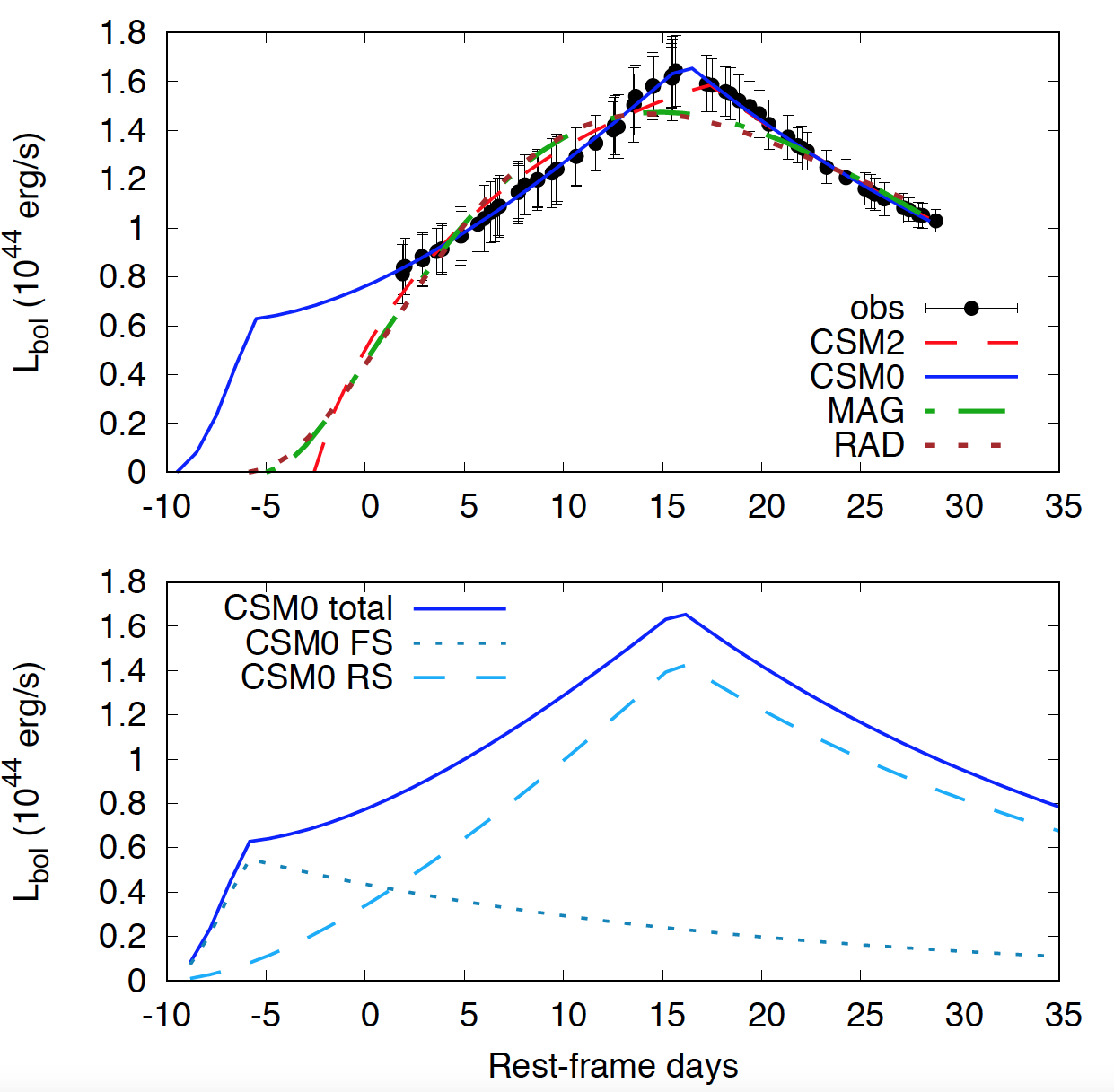
Figure 1.— Upper Panel Bolometric light curve of SN 2017egm from Bose et al. (2017), their figure 7 (black points). The zero of the time axis is arbitrary and the first two data points were omitted (see text). Models computed with MINIM are shown with input from radioactive decay of ⁵⁶Ni and ⁵⁶Co (RAD; brown dash) and from magnetar input (MAG; green long/short dash). Also shown are models based on CSI with two density profiles corresponding to a steady state wind $s=2$ (CSM2; red dash) and to a constant density $s=0$ with an outer cutoff (CSM0; blue). Model parameters are given in Table 1. The constant-density CSI model gives the best fit overall. Lower Panel Decomposition of the MINIM best-fit constant density CSI model from Figure the upper panel showing the effect of the forward shock (green dash) the reverse shock (blue dash) and total luminosity (red). The zero point of the time axis is arbitrary. See the online version for color.

Figure 2 shows a variety of light curve fits using TigerFit (again excluding the first two data points). The parameters corresponding to the results given in Figure 2 are given in Table 1. These models formally assume a region of constant density ($\delta=0$) in the inner region of the ejecta. Models based purely on radioactive decay (upper left) or on a magnetar (upper right) are again clearly inadequate to capture the sharp peak of SN 2017egm. Models with pure CSI (next two panels) give sharp peaks and decent fits. The model with constant density CSM ($s=0$; left panel) gives an especially good fit. For this model, the break when the shock reaches optically-thin regions occurs prior to the earliest data. With appropriate choice of parameters, the model peak representing the break in slope when the reverse shock reaches the interior of the ejecta fits the data very well. This model requires an inner-shell radius of $\sim 6\times 10^{13}$ cm for a hydrogen-poor opacity of 0.2 cm² g^-1 with a mass of $\sim 30$ M_⊙ exploding with an energy of $\sim 5\times 10^{51}$ erg colliding with a CSM of $\sim 0.6$ M_⊙. The CSM shell has an outer radius of $2.1\times 10^{14}$ cm corresponding to a density of $3.1\times 10^{-11}$ g cm^-3. The parameters of this fit are very similar to those derived from the pure CSI model based on MINIM given in Table 1. The model with a wind-like CSM profile (right panel) again gives a somewhat poorer fit.

Models with constant density CSM and a modicum of decay or magnetar input (lower two left-hand panels) also give good fits to the observed light curve at the expense of greater parameter degeneracy. These models formally allowed about 1 M_⊙ of ⁵⁶Ni and a field of $\sim 10^{14}$ G, respectively. In these cases, the break to less steep slope when the shock reaches optically-thin depths in the CSM and the break when the reverse shock reaches the inner limits of the ejecta both occur near maximum light in a manner that still approximately captures the sharp peak observed in SN 2017egm. The hybrid models with wind-like CSM profiles (lower two right-hand panels) provide less good fits. In addition to the poor fit, the model powered solely by radioactive decay (RAD) is unphysical because it requires substantially more ⁵⁶Ni than the ejecta mass. The pure magnetar model (MAG) requires a rather small ejecta mass. The model with $s=2$ CSM and magnetar input rises after $\sim 40$ d because the effects of the CSM input die out while the magnetar input continues for this particular model that otherwise showed the lowest $\chi^{2}/\text{d.o.f.}$ value in TigerFit for this class of models.

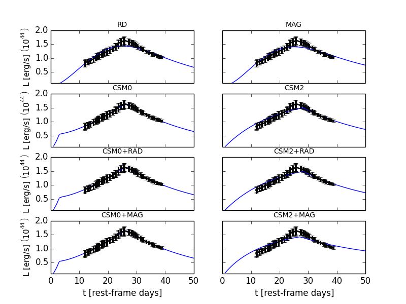
Figure 2.— Bolometric light curve of SN 2017egm from Bose et al. (2017) as in Figure 1 (black points). Fits of the ⁵⁶Ni decay (RAD), magnetar (MAG), CSM models with constant density (CSM0) and wind-like profiles (CSM2) and hybrid models with combined inputs are given by the blue curves. See text for discussion. See the online version for color.

4. Discussion and Conclusions

The nearby SLSN I SN 2017egm displays a rather special quasi-bolometric light curve for the 15 d before and after peak with a sharp peak separating the linear rise from the linear decline. Both radioactive decay models and magnetar models give rounded light curves with smooth peaks. In contrast, models based on CSI can, in principle, yield roughly linear rise and decline joined at a sharp peak. We note that other treatments can give smoother transitions between epochs of CSI models (Moriya et al., 2013). In our models, the eruption of the forward shock from the CS shell causes an early small break in the slope of the light curve. In our models, the abrupt change in slope at peak light corresponds to the epoch when the reverse shock reaches the innermost ejecta. The subsequent lingering exponential decline comes from the continued diffusive release of energy from deeper layers. We have presented several models showing that CSI can account for the light curve shape of SN 2017egm around maximum light, including models in which the CSI is abetted by a modest input from radioactive decay or a magnetar.

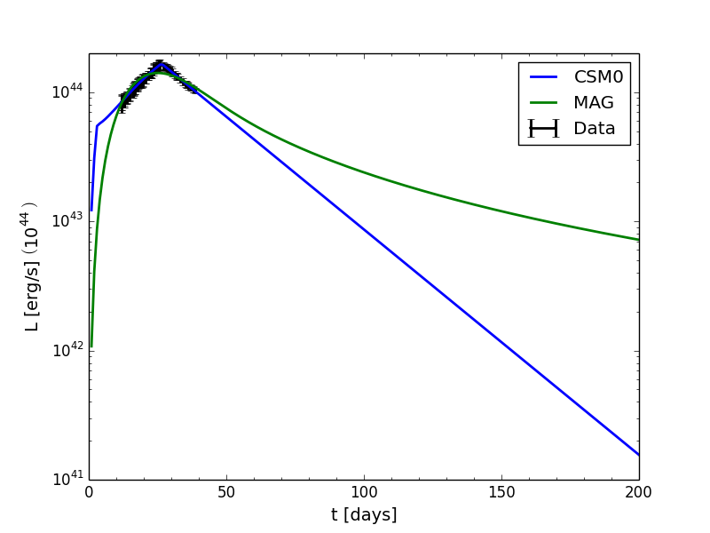
Figure 3.— Bolometric light curve of SN 2017egm from Bose et al. (2017) as in Figure 1 (black points) with best-fit CSI and magnetar models from Figure 2 extrapolated to longer time periods. The diffusive exponential decline of the CSI model (blue) is predicted to fall off much more steeply than the power law of the simple magnetar model (red). See the online version for color.

The data currently available to us mitigate against pure radioactive decay or pure magnetar models, but the data only span about 30 days around peak. A critical test will be the subsequent behavior of the light curve. The bolometric light curve of a radioactive-decay model follows certain systematics driven by the physics of the weak interactions. At late times, the bolometric light curves of basic dipole-driven magnetar models are predicted to decay like $t^{-2}$. Both the decay models and the magnetar models can be altered by leakage of gamma-rays, positrons, or magnetar input at the expense of added fitting parameters. CSM models are intrinsically bedeviled by a profusion of fitting parameters, but they do have characteristics that allow sharp breaks in the light curve. It is possible that SN 2017egm is displaying some of those characteristics. Again, more extensive data on the decline will provide important constraints on CSI models.

Figure 3 shows the extrapolation of our best-fit TigerFit CSM0 and MAG models to 200 days. At face value, photometric monitoring should easily discriminate these two basic models, with CSM0 decaying exponentially, and MAG decaying as a power-law, $t^{-2}$. In practice, variations in both models might decrease the contrast. Our simple MAG model ignores the dynamical effects of a wind-blown shell (Kasen et al., 2016) or leakage effects (Nicholl et al., 2017b). As the luminosity declines, some input from ⁵⁶Co decay might contaminate either model. Nevertheless, the contrast expected between the two classes of models is very large.

The data on SN 2017egm and our models suggest that CSM is a major factor. The issue of whether CSM could be active in SLSN I despite the lack of evidence for narrow nebular lines was raised in Chatzopoulos et al. (2012) and discussed in some more detail in Chatzopoulos et al. (2013). This remains a controversial issue, to which SN 2017egm may bring some clarity. The slowly-declining SLSN I are often characterized by irregularities in the light curve that are most straightforwardly attributed to CSI (De Cia et al., 2017). If a class of SLSN or a single example in the case of SN 2017egm argue for CSI despite the lack of narrow lines, then the implication of the lack of narrow lines must be reconsidered in all SLSN I.

Table 1Fitting and derived parameters for the light curve models of SN 2017egm

Parameter	RAD	MAG	CSM0	CSM2	CSM0+RAD	CSM2+RAD	CSM0+MAG	CSM2+MAG
			MINIM (Figure 1)
$M_{\rm Ni}$ ($M_{\odot}$)	11.2 (0.5)	–	–	–
$M_{\rm ej}$ ($M_{\odot}$)	4.61 (0.28)	4.33 (0.22)	29.7 (1.7)	50.2 (6.3)
$E_{\rm SN}$ ($10^{51}$ erg)	11.1 (0.7)	10.4 (0.5)	5.7 (0.3)	6.6 (0.8)
$P_{0,\rm mag}$ (ms)	–	3.91 (0.08)	–	–
$B_{\rm mag}$ ($10^{14}$ G)	–	3.20 (0.07)	–	–
$R_{\rm p}$ ($10^{13}$ cm)	–	–	8.9 (0.6)	9.6 (3.9)
$\dot{M}$ ($M_{\odot}$ yr-1)	–	–	0.014 (0.001)	0.076 (0.003)
			TigerFit (Figure 2)
$M_{\rm Ni}$ ($M_{\odot}$)	13.5	–	–	–	1.0	0.7	–	–
$M_{\rm ej}$ ($M_{\odot}$)	4.0	3.4	30.0	63.7	30.0	63.7	30.5	63.9
$E_{\rm SN}$ ($10^{51}$ erg)	9.6	8.2	5.0	6.0	5.0	6.0	4.9	4.2
$P_{0,\rm mag}$ (ms)	–	4.0	–	–	–	–	6.1	3.0
$B_{\rm mag}$ ($10^{14}$ G)	–	0.6	–	–	–	–	0.8	0.6
$R_{\rm p}$ ($10^{13}$ cm)	–	–	6.0	1.0	6.0	1.0	5.0	1.2
$\dot{M}$ ($M_{\odot}$ yr-1)	–	–	0.11	0.8	0.10	0.77	0.08	0.8
$\delta$	–	–	0	0	0	0	0	0
$n$	–	–	11	12	11	12	11	12
$s$	–	–	0	2	0	2	0	2
$\chi^{2}/\text{d.o.f.}$	0.61	0.87	0.02	0.63	0.03	0.65	0.03	1.38

Note. — RAD: radioactive decay diffusion model, MAG: magnetar spin–down model, CSM0: circumstellar interaction model with $s=$ 0, CSM2: circumstellar interaction model with $s=$ 2, CSM0+RAD: hybrid circumstellar interaction ($s=$ 0) and radioactive decay model, CSM2+RAD: hybrid circumstellar interaction ($s=$ 2) and radioactive decay model, CSM0+MAG: hybrid circumstellar interaction ($s=$ 0) and magnetar spin–down model, CSM2+MAG: hybrid circumstellar interaction ($s=$ 2) and magnetar spin–down model.

References

- Arnett (1982) Arnett, W. D. 1982, ApJ, 253, 785
- Bose et al. (2017) Bose, S., Dong, S., Pastorello, A., et al. 2017, arXiv:1708.00864
- Chatzopoulos et al. (2012) Chatzopoulos, E., Wheeler, J. C., & Vinko, J. 2012, ApJ, 746, 121
- Chatzopoulos et al. (2013) Chatzopoulos, E., Wheeler, J. C., Vinko, J., Horvath, Z. L., & Nagy, A. 2013, ApJ, 773, 76
- Chen et al. (2013) Chen, T.-W., Smartt, S. J., Bresolin, F., et al. 2013, ApJL, 763, L28
- Chen et al. (2017) Chen, T.-W., Schady, P., Xiao, L., et al. 2017, arXiv:1708.04618
- De Cia et al. (2017) De Cia, A., Gal-Yam, A., Rubin, A., et al. 2017, arXiv:1708.01623
- Dong et al. (2017) Dong, S., Bose, S., Chen, P., et al. 2017, The Astronomer’s Telegram, 1049,
- Izzo et al. (2017) Izzo, L., Thöne, C. C., García-Benito, R., et al. 2017, arXiv:1708.03856
- Kasen et al. (2016) Kasen, D., Metzger, B. D., & Bildsten, L. 2016, ApJ, 821, 36
- Leloudas et al. (2015) Leloudas, G., Schulze, S., Krühler, T., et al. 2015, MNRAS, 449, 917
- Lunnan et al. (2014) Lunnan, R., Chornock, R., Berger, E., et al. 2014, ApJ, 787, 138
- Lunnan et al. (2017) Lunnan, R., Chornock, R., Berger, E., et al. 2017, arXiv:1708.01619
- Moriya et al. (2013) Moriya, T. J., Blinnikov, S. I., Tominaga, N., et al. 2013, MNRAS, 428, 1020
- Neill et al. (2011) Neill, J. D., Sullivan, M., Gal-Yam, A., et al. 2011, ApJ, 727, 15
- Nicholl et al. (2017a) Nicholl, M., Berger, E., Margutti, R., et al. 2017, ApJL, 845, L8
- Nicholl et al. (2017b) Nicholl, M., Guillochon, J., & Berger, E. 2017, arXiv:1706.00825
- Perley et al. (2016) Perley, D. A., Quimby, R. M., Yan, L., et al. 2016, ApJ, 830, 13
- Quimby et al. (2007) Quimby, R. M., Aldering, G., Wheeler, J. C., et al. 2007, ApJL, 668, L99
- Quimby et al. (2011) Quimby, R. M., Kulkarni, S. R., Kasliwal, M. M., et al. 2011, Nature, 474, 487
- Stoll et al. (2011) Stoll, R., Prieto, J. L., Stanek, K. Z., et al. 2011, ApJ, 730, 34
- Xiang et al. (2017) Xiang, D., Song, H., Wang, X., et al. 2017, The Astronomer’s Telegram, 1044,