Statistical symmetry restoration in fully developed turbulence: Renormalization group analysis of two models

Abstract

In this paper we consider the model of incompressible fluid described by the stochastic Navier-Stokes equation with finite correlation time of a random force. Inertial-range asymptotic behavior of fully developed turbulence is studied by means of the field theoretic renormalization group within the one-loop approximation. It is corroborated that regardless of the values of model parameters and initial data, the inertial-range behavior of the model is described by limiting case of vanishing correlation time. It indicates that the Galilean symmetry of the model violated by the “colored” random force is restored in the inertial range. This regime corresponds to the only nontrivial fixed point of the renormalization group equation. The stability of this point depends on the relation between the exponents in the energy spectrum ${\cal E}\propto k^{1-y}$ and the dispersion law $\omega\propto k^{2-\eta}$. The second analyzed problem is the passive advection of a scalar field by this velocity ensemble. Correlation functions of the scalar field exhibit anomalous scaling behavior in the inertial-convective range. We demonstrate that in accordance with Kolmogorov’s hypothesis of the local symmetry restoration, the main contribution to the operator product expansion is given by the isotropic operator, while anisotropic terms should be considered only as corrections.

I Introduction

The very important phenomenological concepts in the theory of fluid turbulence is the concept of the statistical symmetry restoration Legacy ; LegacyD . The Navier-Stokes (NS) equation describing fluid dynamics possesses a number of symmetries: translational and rotational covariance and covariance with respect to Galilean transformation. Some of these symmetries are violated inevitably by the experimental setup or, speaking mathematically, by initial and boundary conditions. Moreover, some of the remaining symmetries can be broken spontaneously as the Reynolds number $\mathrm{Re}$ increases; see Refs. Legacy ; LegacyD for detailed discussions and examples.

However, for fully developed turbulence ($\mathrm{Re}\gg 1$) these symmetries can be restored in the statistical sense, that is, for various correlation or structure functions and in a proper range of scales (inertial interval). This concept dates back to Kolmogorov’s idea of locally isotropic turbulence Monin ; K41a ; K41b ; K41c and is intuitively explained by the idea of the Richardson cascade Richardson . According to Richardson the energy fed into the system at very large scales is transferred downscales through numerous fractions of turbulent eddies. Thus, eventually, at small scales the system “forgets” about details of the energy pumping; see Refs. E84 ; S97 ; P98 ; P99 ; P00 ; B96 and review paper P05 for some examples of such behavior.

In spite of their great value, phenomenological theories might appear to be inaccurate or even incorrect. Nowadays it is widely accepted that due to phenomenon of intermittency, correlation functions of developed turbulence depend on the integral (external) scale $L$, which is in disagreement with the classical Kolmogorov K41 theory. In particular, the equal-time structure functions of the velocity field or those of advected scalar field are described by an infinite set of independent anomalous exponents; see Refs. Legacy ; LegacyD for detailed discussion and references.

Thus, it is desirable to test predictions of phenomenological theories on the basis of certain specific models and by means of some analytical tools. An example of such simplified but very fruitful model is provided by Kraichnan’s rapid-change model, where the existence of anomalous scaling was demonstrated by several approaches, and the corresponding exponents were calculated both numerically and analytically, within controlled approximations and regular perturbation expansions; see Ref. FGV for a review and references.

The effective approach to the discussed problem is the field theoretic renormalization group (RG), see the monographs Zinn ; Vasiliev ; Tauber and review paper HHL . Kraichnan’s model allows one to construct a controlled expansion for the anomalous exponents, which is similar to the famous epsilon-expansion in the theory of critical state AAV ; P96 . The practical calculations were performed up to the third (three-loop) order cube . What is more important, the model can be generalized to the more realistic cases: finite correlation time and non-Gaussianity of the advecting velocity field FinTime ; AKens ; JphysA ; FinTimeEta ; Lanotte2-mod2 ; AGM , strong anisotropy R2 ; R2M ; Arp ; VectorN , compressibility Tomas ; Marian2C ; AK14 ; AK15 , helicity HZ ; MMZ ; MMZR ; R1 , and so on Marian ; AntGul2012 ; Marian2 ; AK2 . Admittedly, in application to the NS equation itself the RG method has so far restricted success turbo .

In this paper, we study two analytic examples of statistical symmetry restoration in fully developed turbulence, based on the stochastic NS equation. The fluid is assumed to be incompressible. As it is standard for the RG approach, we consider the NS equation subjected to an external stirring random force with the prescribed Gaussian statistics. In majority of studies, the random force is $\delta$ correlated in time (“white noise”), which is dictated by the Galilean symmetry. Here, we do not assume this symmetry in advance and choose the force with finite correlation time (“colored noise”). This gives much more freedom for the form of the correlation function. For definiteness, we take the random force as the variant of the Ornstein-Uhlenbeck process OU1 ; OU2 . Such statistics were used earlier in Ref. NonG for generation of the velocity field itself. In our case, however, the velocity field is not described within a certain statistical ensemble but is determined by the real nonlinear NS equation. Various aspects of finite correlation time of a random noise in stochastic dynamics were discussed earlier, e.g., in Refs. Carati ; CaratiV ; CaratiK ; Astro1 ; Astro2 .

The model can be reformulated as a multiplicatively renormalizable quantum field theory. It is well known that in such case the possible large-scale, long-distance asymptotic regimes are associated with infrared (IR) attractive fixed points of the RG equations. We perform the leading-order (one-loop) calculation and show that the only nontrivial IR attractive fixed point corresponds to the $\delta$ correlated force. From a physical point of view it means that the Galilean symmetry is restored immediately in the IR range, which is in accordance with the general concept.

The second problem is the passive advection of a scalar quantity (temperature, density of a pollutant, etc.) in a turbulent fluid. The latter is described by the previously studied stochastic NS field. In view of the aforementioned result, the random force is taken to be $\delta$ correlated in time. The scalar field is governed by the standard advection-diffusion equation with a random force. The latter maintains the steady state and is a source of a large-scale anisotropy. The corresponding field theory is renormalizable and possesses the only IR attractive fixed point. It is well known that correlation functions of the scalar field demonstrate anomalous scaling, so that the K41 theory does not hold; see Ref. Kim for two-loop calculation in the isotropic case. In the RG approach, the anomalous exponents are identified with scaling dimensions of certain composite fields (“composite operators” in the quantum-field terminology). For anisotropic case, it is natural to expand the structure functions in spherical harmonics $Y_{lm}$, where $l$ can be viewed as a degree of anisotropy of the given contribution. In the present model, a special anomalous exponent can be assigned to any contribution.

In this paper we restrict ourselves to the pair correlation function and calculate anomalous exponents in the one-loop approximation for all $l$. It turns out, that these exponents exhibit a kind of hierarchy: they increase monotonically with $l$. As a result, turbulence becomes less and less anisotropic in the depth of the inertial range, and the leading-order term is given by the isotropic contribution. Similar effect was observed earlier in the models of scalar and vector advection by “synthetic” Gaussian velocity fields, see Refs. LM ; ALM ; FinTime ; AHMMG and literature cited therein.

The paper is organized as follows. In Sec. II a detailed description of the stochastic Navier-Stokes equation for an incompressible fluid is given. Sec. III is devoted to the field theoretic formulation of the model and the corresponding diagrammatic technique. In particular, possible types of divergent Green’s functions are discussed. In Sec. IV the renormalizability of the model is proven. One-loop explicit expressions for the renormalization constants are presented and RG functions (anomalous dimensions and $\beta$ functions) are derived and analyzed. In Sec. V the IR asymptotic behavior, obtained by solving the RG equations, is discussed. It is shown that, depending on two exponents $y$ and $\eta$ that describe the energy spectrum and dispersion law of the velocity field, the RG equations exhibit two nontrivial fixed points, but only one of them is stable in the IR region. This means that the Galilean symmetry of the model violated by the colored random force is restored in the inertial range. In Sec. VI the corresponding scaling dimensions of the fields are presented.

In Sec. VII an advection of a passive scalar field by the incompressible velocity field which obeys the NS equation is analyzed. The field theoretic formulation of the full model is presented. The existence of a scaling regime in the IR range is established. In Sec. VIII the operator product expansion for the pair correlation function is carried out. Sec. IX is devoted to the renormalization of composite operators. An inertial-range behavior of the correlation functions is studied. It is shown that the leading terms of the inertial-range behavior are determined by the contributions which correspond to the isotropic terms.

Sec. X is reserved for conclusions. The main one is that the Galilean symmetry and isotropy, broken by introducing the external stochastic force with finite correlation time and by distinguished direction, are restored in the statistical sense (for measurable quantities) in the inertial range of fully developed turbulence.

Appendix A contains detailed calculations of the diagrams, needed to perform multiplicative renormalization of the model of incompressible fluid. Appendix B contains all calculations related to the renormalization procedure and calculation of anomalous dimensions of the composite operators of advected field.

II Description of the model

One of the possible approaches to model fully developed turbulence within the framework of some microscopic model is to study the stochastic Navier-Stokes equation with a random external force Legacy ; LegacyD . It has the form

$$\partial_{t}v_{k}+(v_{i}\partial_{i})v_{k}+\partial_{k}\wp=\nu_{0}\partial^{2}v_{k}+\phi_{k},$$ (1)

where $v_{i}(x)$ is a transverse (owing to the incompressibility) velocity field, $x\equiv\left\{t,{\bm{x}}\right\}$, $\partial_{t}\equiv\partial/\partial t$, $\partial_{i}\equiv\partial/\partial x_{i}$, $\nu_{0}$ is the molecular kinematic viscosity, $\partial^{2}=\partial_{i}\partial_{i}$ is the Laplace operator, $\wp=-\partial^{-2}(\partial_{i}v_{l})(\partial_{l}v_{i})$ is the pressure per unit mass, and $\phi_{k}$ is the external force per unit mass. Since the field $v_{i}(x)$ is incompressible we may use special units in which the density $\rho(x)=1$. The turbulence is modeled by the force $\phi_{k}$, which is assumed to be a random variable. In stochastic formulation of the problem it mimics the input of energy into the system from the outer large scale $L$. Without loss of generality the correlations of the random force $\phi_{k}$ in Fourier space read Monin

$$\left\langle\phi_{i}(\omega,{\bm{k}})\ \phi_{j}(\omega^{\prime},{\bm{k}}^{\prime})\right\rangle\propto\delta(\omega+\omega^{\prime})\delta({\bm{k}}+{\bm{k}}^{\prime})P_{ij}({\bm{k}})D_{\phi}(\omega,k),$$ (2)

where $P_{ij}({\bm{k}})=\delta_{ij}-k_{i}k_{j}/k^{2}$ is the transverse projector and two $\delta$ functions are consequences of the translational invariance.

The Galilean invariance for the model requires the function $D_{\phi}(\omega,k)$ in Eq. (2) to be $\delta$ correlated in time turbo . Nevertheless, it is very intriguing to consider such a model with a colored noise, i.e., with finite and not small correlation time, which is much more realistic from the physical point of view. In general case this modification breaks the Galilean invariance, so the main question of the paper is the following: is this symmetry restored in statistical sense for relevant measurable quantities?

The random force $\phi_{i}$ is simulated in the present paper by the statistical ensemble being a particular case of the Ornstein-Uhlenbeck process: it is assumed to be Gaussian and homogeneous, with zero mean and correlation function OU1 ; OU2 ; NonG

$$\left\langle\phi_{i}(t,{\bm{x}})\phi_{j}(t^{\prime},{\bm{x}^{\prime}})\right\rangle=D_{0}\int\frac{d\omega}{2\pi}\int_{k>m}\frac{d{\bm{k}}}{(2\pi)^{d}}\ P_{ij}({\bm{k}})\frac{k^{8-d-(y+2\eta)}}{\omega^{2}+\nu_{0}^{2}u_{0}^{2}k^{4-2\eta}}\ e^{i{\bm{k}\cdot(\bm{x}-\bm{x}^{\prime})}-i{\omega(t-t^{\prime})}}.$$ (3)

Here $k\equiv|{\bm{k}}|$ is the wave number, $D_{0}>0$ is an amplitude factor, $d$ is an arbitrary (for generality) dimension of ${\bm{x}}$ space, $1/m$ is the integral turbulence scale, related to the stirring. The function (3) involves two independent exponents $y$ and $\eta$. The first one describes the energy spectrum of the velocity in the inertial range ${\cal E}\propto k^{1-y}$. The second exponent is related to the dispersion law: the correlation time of the momentum $k$ scales as $k^{-2+\eta}$. In the RG approach these two exponents play the role of two formal expansion parameters. A new parameter $u_{0}$ is introduced for the dimensionality reasons. Such ensemble was employed in some systems, studied in Refs. AKens ; FinTime ; FinTimeEta . It was shown that depending on the values of the exponents $y$ and $\eta$, the model reveals various types of inertial-range scaling regimes with nontrivial anomalous exponents, which were explicitly derived to the first FinTime and second FinTimeEta orders of the double expansion in $y$ and $\eta$.

Depending on the parameter $u_{0}$, the function (3) demonstrates two interesting limiting cases: if $u_{0}\to 0$, the situation corresponds to the independent of time (“frozen”) random force, the case $u_{0}\to\infty$ corresponds to the zero-time correlated model. The relations

$$D_{0}/\nu_{0}^{5}u_{0}^{2}=g_{0}\propto\Lambda^{y+2\eta},\quad u_{0}\propto\Lambda^{\eta}$$ (4)

define the coupling constant $g_{0}$, which plays the role of the expansion parameter in the ordinary perturbation theory, and the characteristic ultraviolet (UV) momentum scale $\Lambda$. The parameter $u_{0}$ introduced in Eq. (3) is written in the first expression for the calculation reasons, in particular it is convenient in case of large $u_{0}$.

III Field theoretic formulation of the model

According to the general theorem Zinn ; Vasiliev ; Tauber , the stochastic problem (1) and (3) is equivalent to the field theoretic model with a doubled set of fields $\Phi\equiv\left\{v_{i}^{\prime},v_{i}\right\}$ and the De Dominicis-Janssen action functional, which can be written in a compact form as

$${\cal S}_{{\bm{v}}}(\Phi)=\frac{1}{2}v_{i}^{\prime}D_{ik}v_{k}^{\prime}+v^{\prime}_{k}\left[-\partial_{t}-(v_{i}\partial_{i})+\nu_{0}\partial^{2}\right]v_{k}.$$ (5)

Here $D_{ik}$ is the correlator (3) and we employ a condensed notation, in which integrals over the spatial variable ${\bm{x}}$ and the time variable $t$, as well as summation over the repeated indices, are omitted and assumed implicitly

$$v^{\prime}_{k}\partial_{t}{v}_{k} = \sum_{k=1}^{d}\int dt\int d{\bm{x}}\ v_{k}^{\prime}(t,\bm{x})\partial_{t}v_{k}(t,\bm{x}),$$ (6)

$$v^{\prime}_{i}D_{ik}v^{\prime}_{k} = \sum_{i,k=1}^{d}\int dt\int dt^{\prime}\int d{\bm{x}}\int{\mathrm{d}}{\bm{x}^{\prime}}\ v_{i}(t,\bm{x})D_{ik}(t-t^{\prime},\bm{x}-\bm{x}^{\prime})v_{k}(t^{\prime},\bm{x}^{\prime}).$$

Since the auxiliary field $v^{\prime}_{k}$ is transverse, i.e. $\partial_{k}v^{\prime}_{k}=0$, the pressure term in expression (5) can be eliminated using integration by parts

$$v^{\prime}_{k}\partial_{k}\wp=-\wp\partial_{k}v^{\prime}_{k}=0.$$ (7)

Expressions (7) means that the field $v^{\prime}_{k}$ acts as a transverse projector and selects the transverse parts of the expressions with which it is contracted.

The field theoretic formulation (5) means that various correlation and response functions of the original stochastic problem are represented by functional averages over the full set of fields with the functional weight $\exp{\cal S}_{{\bm{v}}}(\Phi)$, and in this sense they can be interpreted as the Green’s functions of the field theoretic model Zinn ; Vasiliev ; Tauber . The perturbation theory of the model can be constructed according to the well-known Feynman diagrammatic expansion. Bare propagators are read off from the inverse matrix of the Gaussian (free) part of the action functional, while a nonlinear part of the differential equation (1) leads to the interaction vertex $-v_{k}^{\prime}(v_{i}\partial_{i})v_{k}$. The propagator functions in the frequency-momentum representation read

$$\left\langle v_{i}v_{j}\right\rangle_{0} = D_{0}\ \frac{k^{8-d-(y+2\eta)}}{\omega^{2}+\nu_{0}^{2}u_{0}^{2}k^{4-2\eta}}\frac{P_{ij}({\bm{k}})}{\omega^{2}+\nu_{0}^{2}k^{4}},$$ (8)

$$\left\langle v_{i}v^{\prime}_{j}\right\rangle_{0} = \frac{P_{ij}({\bm{k}})}{-i\omega+\nu_{0}k^{2}};$$ (9)

the triple vertex corresponds to the expression

$$V_{ijl}=i\left(\delta_{il}k_{j}+\delta_{ij}k_{l}\right).$$ (10)

Due to the incompressibility the derivative in the vertex can be moved onto the field $v_{i}^{\prime}$, hence, $k_{i}$ is the momentum of the field $v^{\prime}_{i}$. A graphical representation of the propagator functions and interaction vertex are depicted in Fig. 1 and Fig. 2, respectively. From now on, the end of a solid line without a slash denotes the field $v_{i}$, the end of a solid line with a slash denotes the field $v_{i}^{\prime}$.

Figure 1: Graphical representation of the bare propagators in the model (5).

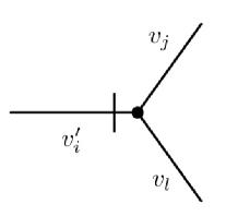
Figure 2: Graphical representation of the interaction vertex in the model (5).

The analysis of UV divergences is based on the analysis of the 1-irreducible Green’s functions. In case of dynamical models Vasiliev two independent scales (the time scale $T$ and the length scale $L$) have to be introduced:

$$[F]\sim[T]^{-d_{F}^{\omega}}[L]^{-d_{F}^{k}},$$ (11)

where $d_{F}^{\omega}$ and $d_{F}^{k}$ are frequency and momentum dimensions of the quantity $F$, respectively. The normalization conditions are

$$d_{k}^{k}=-d_{x}^{k}=d_{\omega}^{\omega}=-d_{t}^{\omega} =1,$$ (12)

$$d_{\omega}^{k}=d_{t}^{k}=d_{k}^{\omega}=d_{x}^{\omega} =0.$$

Based on $d_{F}^{k}$ and $d_{F}^{\omega}$ the total canonical dimension $d_{F}=d_{F}^{k}+2d_{F}^{\omega}$ can be introduced, which in the renormalization theory of the dynamic models plays the same role as the conventional (momentum) dimension does in the static problems.

The canonical dimensions for the model (5) are given in Table 1, including the renormalized parameters (without the subscript “$0$”), which will be introduced later. The parameters $\theta$, $\theta^{\prime}$, $\kappa$, and $w$ are connected with the problem of the advection of scalar field and will be used in Secs. VII – IX. From Table 1 it follows that our model is logarithmic (the coupling constants $g_{0}\sim[L]^{-y}$ and $u_{0}\sim[L]^{-\eta}$ are simultaneously dimensionless) at $y=\eta=0$, so in the minimal subtraction (MS) scheme, which we use in this paper, the UV divergences in the Green’s functions manifest themselves as poles in $y$, $\eta$ and their linear combinations.

The total canonical dimension of an arbitrary 1-irreducible Green’s function $\Gamma_{N_{\Phi}}=\langle\Phi\dots\Phi\rangle_{\rm 1-ir}$ is given by the relation

$$d_{\Gamma}=d+2-\sum_{\Phi}N_{\Phi}d_{\Phi}=d+2-N_{v^{\prime}}d_{v^{\prime}}-N_{v}d_{v}.$$ (13)

Here $N_{\Phi}=\{N_{v},\,N_{v^{\prime}}\}$ are the numbers of corresponding fields entering the function $\Gamma$ and $d_{\Phi}$ is the corresponding total canonical dimension of a field $\Phi$ Zinn ; Vasiliev ; Tauber . The superficial UV divergences the removal of which requires counterterms might be present only in the functions $\Gamma$ for which the formal index of divergence $\delta_{\Gamma}$ (being the value of $d_{\Gamma}$ in the logarithmic theory) is a non-negative integer. Dimensional analysis should be augmented by the following considerations:

(1) In any dynamical model of the type (5) all the 1-irreducible functions without the response field $v_{i}^{\prime}$ necessarily contain closed circuits of retarded propagators similar to (9). Therefore, such functions vanish identically and do not require counterterms.

(2) Using the transversality condition of the field $v_{i}$ we can move the derivative in the vertex $-v_{k}^{\prime}(v_{i}\partial_{i})v_{k}$ from the field $v_{k}$ onto the field $v_{i}^{\prime}$. Therefore, in any 1-irreducible diagram it is always possible to move derivatives onto external “tails” $v_{i}^{\prime}$, which reduces the real index of divergence: $d^{\prime}_{\Gamma}=d_{\Gamma}-N_{v^{\prime}}$.

Table 1: Canonical dimensions of the fields and parameters in the model (5).

$F$	$\bm{v}^{\prime}$	$\bm{v}$	$\theta$	$\theta^{\prime}$	$M,m,\mu,\Lambda$	$\nu,\nu_{0}$, $\kappa$, $\kappa_{0}$	$u,u_{0}$	$g_{0}$	$g$, $w$, $w_{0}$
$d_{F}^{\omega}$	$-1$	$1$	$-1/2$	1/2	$0$	$1$	0	0	0
$d_{F}^{k}$	$d+1$	$-1$	0	$d$	$1$	$-2$	$\eta$	$y$	0
$d_{F}$	$d-1$	$1$	$-1$	$d+1$	$1$	$0$	$\eta$	$y$	0

From Table 1 and Eq. (13) we find that

$$d_{\Gamma}=d+2-dN_{v^{\prime}}-N_{v}.$$ (14)

From this expression we conclude that for any $d>2$, superficial divergences can be present only in the 1-irreducible functions of two types. The first example is the function $\langle v_{\alpha}^{\prime}v_{\beta}\rangle_{\rm 1-ir}$, for which the real index of divergence is $d_{\Gamma}=2$. Another possibility is the function $\langle v_{\alpha}^{\prime}v_{\beta}v_{\gamma}\rangle_{\rm 1-ir}$ with $d_{\Gamma}=1$. This means, that all the UV divergences in our model can be removed by the counterterms of the form $v_{i}\partial^{2}v_{i}$ and $v^{\prime}_{k}(v_{i}\partial_{i})v_{k}$. The Galilean invariance which holds in case of $\delta$ correlated in time function $D_{\phi}(\omega,k)$ forbids the divergence of the vertex $\langle v_{\alpha}^{\prime}v_{\beta}v_{\gamma}\rangle_{\rm 1-ir}$, which we have in our case of the colored noise (3). For $d=2$ a new UV divergence arises in the function $\langle v^{\prime}_{\alpha}v^{\prime}_{\beta}\rangle_{\rm 1-ir}$, and a new counterterm $v_{i}^{\prime}\partial^{2}v_{i}^{\prime}$ should be included Two . This case requires a special treatment, and in the following we assume $d>2$.

The model (5) is multiplicatively renormalizable with two independent renormalization constants $Z_{1}$ and $Z_{2}$; the renormalized action functional has the form

$${\cal S}_{{{\bm{v}}}_{R}}(\Phi)=\frac{1}{2}v_{i}^{\prime}D_{v}v_{k}^{\prime}+v^{\prime}_{k}\left[-\partial_{t}-Z_{1}(v_{i}\partial_{i})+Z_{2}\nu\partial^{2}\right]v_{k}.$$ (15)

Here $g$, $\nu$, and $u$ are the renormalized counterparts of the original (bare) parameters, the function $D_{v}$ is expressed in the renormalized parameters using the relation $g_{0}\nu_{0}^{5}u_{0}^{2}=g\mu^{y+2\eta}\nu^{5}u^{2}$; the reference scale $\mu$ is an additional free parameter of the renormalized theory.

The renormalized action (15) is obtained from the original one (5) by the renormalization of the fields $v\to Z_{v}v$, $v^{\prime}\to Z_{v^{\prime}}v^{\prime}$ and the parameters

$$g_{0}=g\mu^{y}Z_{g},\quad u_{0}=u\mu^{\eta}Z_{u},\quad\nu_{0}=\nu Z_{\nu}.$$ (16)

The renormalization constants in Eqs. (15) and (16) are related as

$$Z_{\nu}=Z_{2},\quad Z_{u}=Z_{2}^{-1},\quad Z_{g}=Z_{1}^{2}Z_{2}^{-3},\quad Z_{v}=Z_{v^{\prime}}^{-1}=Z_{1}.$$ (17)

The renormalization constants are found from the requirement that the Green’s functions of the renormalized model (15), when expressed in renormalized variables, have to be UV finite and can depend only on the completely dimensionless parameters $g,u,d,y$, and $\eta$.

IV Renormalization of the model and RG functions

Let us consider the generating functional of the 1-irreducible Green’s functions

$$\Gamma(\Phi)={\cal S}_{{\bm{v}}}(\Phi)+\widetilde{\Gamma}(\Phi),$$ (18)

where ${\cal S}_{{\bm{v}}}(\Phi)$ is the action functional (5) and $\widetilde{\Gamma}(\Phi)$ is the sum of all the 1-irreducible diagrams with loops.

Hence, one-loop approximation for the 1-irreducible Green’s functions that require UV renormalization provides

$$\langle v_{\alpha}^{\prime}v_{\beta}\rangle_{\rm 1-ir} = \left(i\omega-\nu_{0}p^{2}\right)P_{\alpha\beta}({\bm{p}})+\Sigma_{\alpha\beta},$$ (19)

$$\langle v_{\alpha}^{\prime}v_{\beta}v_{\gamma}\rangle_{\rm 1-ir} = V_{\alpha\beta\gamma}+(\Delta_{1}+\Delta_{2}+\Delta_{3}).$$ (20)

Here, $P_{\alpha\beta}({\bm{p}})$ is the transverse projector, $\Sigma_{\alpha\beta}$ is the self-energy operator, graphical representation for which is depicted in the Fig. 3, $V_{\alpha\beta\gamma}$ is the vertex factor (10), and diagrams $\Delta_{1}$, $\Delta_{2}$, and $\Delta_{3}$ are depicted in Figs. 4a–4c.

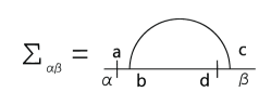
Figure 3: The one-loop approximation of the 1-irreducible response function $\langle v_{\alpha}^{\prime}v_{\beta}\rangle_{\rm 1-ir}$. Greek letters denote external (free) indices of the diagram, Latin letters correspond to internal indices of the vector fields with implied summation.

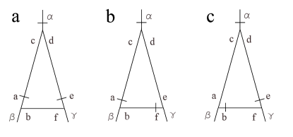
Figure 4: The one-loop approximation of the 1-irreducible function $\langle v_{\alpha}^{\prime}v_{\beta}v_{\gamma}\rangle_{\rm 1-ir}$. Greek letters denote external (free) indices of the diagram, Latin letters correspond to internal indices of the vector fields with implied summation.

The calculation of the renormalization constants $Z_{1}$ and $Z_{2}$ in the one-loop approximation gives

$$Z_{1} = 1-g\frac{1}{d(d+2)}\frac{u}{(u+1)^{3}}\frac{1}{y},$$ (21)

$$Z_{2} = 1-g\frac{1}{d(d+2)}\frac{u^{3}d(d-1)+3u^{2}d(d-1)+2u(d^{2}-d+2)}{4(u+1)^{3}}\frac{1}{y}.$$ (22)

Here, we have introduced a new coupling constant $g\to gS_{d}/(2\pi)^{d}$ with $S_{d}$ being the surface area of the unit sphere in $d$-dimensional space, see Appendixes A.1 and A.2 for details. The corrections of orders $g^{2}$ and higher are neglected.

The relation between the initial and renormalized action functionals $S(\Phi,e_{0})=S^{R}(Z_{\Phi}\Phi,e,\mu)$, where $e$ is the complete set of parameters, yields the fundamental RG differential equation:

$$\biggl{\{}\widetilde{\cal D}_{\mu}+N_{v}\gamma_{v}+N_{v^{\prime}}\gamma_{v^{\prime}}\biggr{\}}\,G^{R}(e,\mu,\dots)=0,$$ (23)

where $G=\langle\Phi\cdots\Phi\rangle$ is the correlation function of the fields $\Phi$; $N_{v}$ and $N_{v^{\prime}}$ are the numbers of the renormalization-requiring fields ${\bm{v}}$ and ${\bm{v}^{\prime}}$, respectively, which are the inputs to $G$; the ellipsis in the expression (23) stands for the other arguments of $G$ (spatial and time variables, etc.). Further, $\widetilde{\cal D}_{\mu}$ is the differential operation $\mu\partial_{\mu}$ taken for fixed $e_{0}$ and expressed in the renormalized variables:

$$\widetilde{\cal D}_{\mu}={\cal D}_{\mu}+\beta_{g}\partial_{g}+\beta_{u}\partial_{u}-\gamma_{\nu}{\cal D}_{\nu}.$$ (24)

Here and below we have denoted ${\cal D}_{x}\equiv x\partial_{x}$ for any variable $x$. The anomalous dimension $\gamma_{F}$ of a certain quantity $F$ (a field or a parameter) is defined as

$$\gamma_{F}=Z_{F}^{-1}\widetilde{\cal D}_{\mu}Z_{F}=\widetilde{\cal D}_{\mu}\ln Z_{F}.$$ (25)

The $\beta$ functions for the two dimensionless coupling constants $g$ and $u$ are

$$\beta_{g} = \widetilde{\cal D}_{\mu}g=g(-y-\gamma_{g}),$$

$$\beta_{u} = \widetilde{\cal D}_{\mu}u=u(-\eta-\gamma_{u}),$$ (26)

where the latter equations result from the definitions and the relations (16).

From the definitions and expressions (21) – (22) for the renormalization constants $Z_{1}$ and $Z_{2}$ one finds

$$\gamma_{1} = g\frac{1}{d(d+2)}\frac{u}{(u+1)^{3}},$$ (27)

$$\gamma_{2} = g\frac{1}{d(d+2)}\frac{u^{3}d(d-1)+3u^{2}d(d-1)+2u(d^{2}-d+2)}{4(u+1)^{3}},$$ (28)

and from the relations (17) it follows that

$$\beta_{g}=g(-y-2\gamma_{1}+3\gamma_{2}),\quad\beta_{u}=u(-\eta+\gamma_{2}).$$ (29)

Eqs. (29) give us full set of $\beta$ functions defining fixed points, which are responsible for asymptotic behavior of correlation and structure functions.

V IR attractive fixed points

One of the basic RG statements is that the asymptotic behavior of the model is governed by the fixed points $\left\{g^{*},u^{*}\right\}$, defined by the equations $\beta_{g}=0$, $\beta_{u}=0$. The type of a fixed point (IR/UV attractive or a saddle point), i.e., the character of the RG flow in the vicinity of the point, is determined by the matrix $\Omega_{ik}=\partial\beta_{i}/\partial g_{k}$ at a given point, where $\beta_{i}$ is the full set of $\beta$ functions and $g_{k}$ is the full set of couplings. For an IR attractive fixed point, the matrix $\Omega$ has to be positive definite, i.e., the real parts of all its eigenvalues have to be positive.

A direct analysis of the $\beta$ functions reveals the existence of the three fixed points: the trivial one and two nontrivial. The free Gaussian fixed point, for which all interactions are irrelevant and no scaling and universality are expected, has the coordinates

$$g^{*}=0,\quad u^{*}=0$$ (30)

and is IR attractive if both $y$ and $\eta$ are negative.

Let us we define $\alpha\equiv\eta/y$ [see Eq. (3)]. If parameter $\alpha$ satisfies the inequalities

$$\frac{1}{3}<\alpha<\frac{1}{3}+\frac{4/3}{3d(d-1)+2},$$ (31)

the system possesses the fixed point $\left\{g^{*},u^{*}\right\}$ with the coordinates

$$u^{*} = \frac{-3+\sqrt{1-\frac{16(\alpha-1)}{d(d-1)(3\alpha-1)}}}{2},$$ (32)

$$g^{*} = d(d+2)\frac{(u^{*}+1)^{3}}{u^{*}}\frac{3\alpha-1}{2}y,$$ (33)

see Fig. 5. However, it turns out that one of the two eigenvalues of the matrix $\Omega$ for this point is negative. This means, that this fixed point is a saddle one, i.e., for any values of $y$ and $\eta$ it is IR attractive only in one of the two possible directions. This fixed point exists for all $d$ except the limit $d\to\infty$, where the inequality (31) has no solution (see details below).

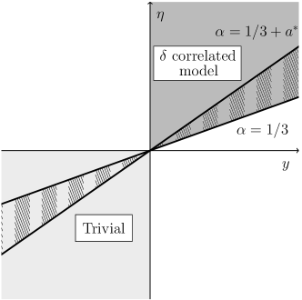
Figure 5: Domains of the existence and IR stability of the fixed points for the model (5) in the plane $(y,\eta)$; $a^{*}=\frac{4/3}{3d(d-1)+2}$. Gray areas correspond to the regions where the trivial and $\delta$ correlated model fixed points are IR attractive; hatched areas which are lying inside the gray ones correspond to the regions where another nontrivial (saddle type) point exists; in white areas there is no IR attractive fixed point.

Another case to be considered is $u^{*}\to\infty$. From Eqs. (3) and (8) it follows that this case corresponds to the previously studied model with the $\delta$ correlated in time random force NS-Zero . Therefore, one should obtain the well-known fixed point of this model. This is indeed the case. To prove this statement it is convenient to pass from the variable $u$ to a variable $x=1/u$. The limit $u\to\infty$ corresponds now to the limit $x\to 0$; the new $\beta$ function is

$$\beta_{x} = \widetilde{\cal D}_{\mu}x=-\frac{1}{u^{2}}\beta_{u}.$$ (34)

If $u^{*}\to\infty$ anomalous dimensions have the following simple form

$$\gamma_{1} = 0,$$ (35)

$$\gamma_{2} = g\frac{d-1}{4(d+2)}.$$ (36)

Therefore, we obtain the new set of $\beta$ functions

$$\beta_{g} = g\left[-y+g\frac{3(d-1)}{4(d+2)}\right],$$ (37)

$$\beta_{x} = x\left[\eta-g\frac{d-1}{4(d+2)}\right].$$ (38)

From Eqs. (37) – (38) it follows that the system possesses the fixed point with the coordinates

$$x^{*}=0,\quad g^{*}=\frac{4(d+2)}{3(d-1)}y,$$ (39)

which coincides with the results of Ref. NS-Zero and is IR attractive for $y>0$ and $\eta>y/3$.

An interesting situation corresponds to the limit $d\to\infty$. The study of the large $d$ behavior of the fluid turbulence is not only an academic interest: one can hope that in this case the intermittency and anomalous scaling disappear or acquire a simple “calculable” form and the finite-dimensional turbulence can be studied within the expansion around this “solvable” limit; hence the idea of expansion in $1/d$, considered in Refs. InfD1 ; InfD2 ; InfD3 ; InfD4 . If $d\to\infty$ the set of the $\beta$ functions (29) reads

$$\beta_{g} = g\left[-y+g\frac{3u(u+2)}{4(u+1)^{2}}\right],$$ (40)

$$\beta_{u} = u\left[-\eta+g\frac{u(u+2)}{4(u+1)^{2}}\right].$$ (41)

Therefore, the system $\beta_{g}=0$, $\beta_{u}=0$ admits several possible solutions. The trivial one is $g^{*}=u^{*}=0$; it corresponds to Eqs. (30) at finite $d$. Another solution is an infinite fixed point

$$x^{*}=0,\quad g^{*}=\frac{4}{3}y,$$ (42)

where $x=1/u$ (see above) and $\beta_{x}$ is given by expression (34). This point is IR attractive for $y>0$ and $\eta>y/3$ and corresponds to Eqs. (39). Furthermore, there is one more solution of the system (40) – (41):

$$g^{*}\frac{u^{*}(u^{*}+2)}{4(u^{*}+1)^{2}}=\frac{y}{3}=\eta,$$ (43)

where both $g^{*}$ and $u^{*}$ are undefined separately. This case corresponds to the saddle type point (32) – (33), but with one significant difference: if $d\to\infty$, two eigenvalues of the matrix $\Omega$ are

$$\lambda_{1}=0;\quad\lambda_{2}=\left.g\frac{u(3u^{2}+9u+8)}{4(u+1)^{3}}\right|_{g^{*},u^{*}}.$$ (44)

Eqs. (43) and (44) are in agreement with the results (32) – (33) for finite $d$. If $d\to\infty$, there is no solution for inequality (31), and two hatched triangles, denoting the possible areas of existence of this point, degenerate into one line $\eta=\frac{y}{3}$ (see Fig. 5). At the same time one of the two eigenvalues, which was negative at finite $d$, tends to zero. This means, that we have not a point, but a line $\eta=\frac{y}{3}$ with zero velocity along it, which is (and was at finite $d$) IR attractive in the perpendicular direction. It is very intriguing phenomenon. On the one hand, there is a continuous limit from finite $d$ to the case $d\to\infty$. Moreover, the expression $\lim_{d\to\infty}\lambda_{1}=0$ can be checked directly from the original $\beta$ functions at the fixed point (32) – (33). On the other hand, the saddle type point, which can be reached only if the initial data (both position and velocity) are very specific and allow it, transforms into an IR attractive line, which will be achieved for any initial data.

The results presented in this section are based on the explicit form of the $\beta$ functions (27) – (29) derived within the leading one-loop approximation. They exhibit a very fine structure and can well appear to be sensitive to inclusion of higher-order corrections. This interesting issue lies beyond the scope of our discussion and will be a subject of further investigation.

VI Critical dimensions

In the leading order of the IR asymptotic behavior, the Green’s functions satisfy the RG equation with the substitution $g\to g^{*}$ and $u\to u^{*}$. This property together with canonical scale invariance gives us the critical dimensions of the fields in the model, which, in fact, govern the asymptotic behavior of arbitrary correlation functions

$$\Delta_{F}=d^{k}_{F}+\Delta_{\omega}d^{\omega}_{F}+\gamma_{F}^{*},\quad{\rm where}\quad\Delta_{\omega}=-\Delta_{t}=2-\gamma_{\nu}^{*}.$$ (45)

Here, $\Delta_{F}$ denotes the critical dimension of the quantity $F$, while $\Delta_{t}$ and $\Delta_{\omega}$ are the critical dimensions of time and frequency. The symbol $\gamma_{F}^{*}$ denotes the value $\gamma_{F}$ at the fixed point.

If $u^{*}\to\infty$ one obtains the exact answers (with no corrections of orders $y^{2}$ and higher)

$$\Delta_{v}=1-y/3,\quad\Delta_{v^{\prime}}=d-1+y/3,$$ (46)

which are in agreement with Ref. NS-Zero .

The saddle fixed point (32) – (33) gives

$$\Delta_{v}=1+\frac{\eta-y}{2},\quad\Delta_{v^{\prime}}=d-1+\frac{\eta-y}{2}.$$ (47)

The latter dimensions have higher-order corrections $y^{n}\eta^{m}$ with $n+m\geqslant 2$. Evaluation of these corrections requires the consideration beyond the one-loop approximation.

VII Advection of passive scalar fields

Let us consider a passive advection of a scalar field $\theta(x)\equiv\theta(t,{\bm{x}})$, which satisfies the stochastic differential equation

$$\partial_{t}\theta+\partial_{i}(v_{i}\theta)=\kappa_{0}\partial^{2}\theta+f_{\theta}.$$ (48)

Eq. (48) describes the advection of a density field, e.g., density of a pollutant. The advection of a tracer field (temperature, specific entropy, or concentration of the impurity particles) differs from this case by the transformation $\partial_{i}(v_{i}\theta)\to(v_{i}\partial_{i})\theta$ on the left-hand side of Eq. (48). Therefore, in case of an incompressible carrier flow (i.e., if $\partial_{i}v_{i}=0$) both density and tracer fields are described by the same equation.

The newly introduced coefficient $\kappa_{0}$ is the molecular diffusivity, $\partial^{2}=\partial_{i}\partial_{i}$ is the Laplace operator, $v_{i}(x)$ is the velocity field, which obeys Eq. (1), and $f_{\theta}=f_{\theta}(x)$ is a Gaussian noise with zero mean and given covariance

$$\langle f_{\theta}(x)f_{\theta}(x^{\prime})\rangle=\delta(t-t^{\prime})\,C({\bm{r}}/L_{\theta}),\quad{\bm{r}}={\bm{x}}-{\bm{x}}^{\prime}.$$ (49)

The function $C({\bm{r}}/L_{\theta})$ in Eq. (49) is finite at $({\bm{r}}/L_{\theta})\to 0$ and rapidly vanishes when $({\bm{r}}/L_{\theta})\to\infty$. The expression (49) brings about another external (integral) scale $L_{\theta}$, related to the noise $f_{\theta}$, but henceforth we will not distinguish it from its analog $L=m^{-1}$ in the correlation function of the stirring force (3). The noise simulates effects of initial and boundary conditions of the system.

If the velocity $v_{i}$ obeys the stochastic Navier-Stokes equation (1), the problem (48), (49) is tantamount to the field theoretic model of the full set of fields $\widetilde{\Phi}\equiv\{\theta^{\prime},\theta,v_{i}^{\prime},v_{i}\}$ and the action functional

$${\cal S}(\widetilde{\Phi})={\cal S}_{\theta}(\theta^{\prime},\theta,v_{i})+{\cal S}_{{\bm{v}}}(v_{i}^{\prime},v_{i}),$$ (50)

where the advection-diffusion component

$${\cal S}_{\theta}(\theta^{\prime},\theta,v_{i})=\frac{1}{2}\theta^{\prime}D_{f}\theta^{\prime}+\theta^{\prime}\left[-\partial_{t}\theta-\partial_{i}(v_{i}\theta)+\kappa_{0}\partial^{2}\theta\right]$$ (51)

is the De Dominicis-Janssen action for the stochastic problem (48), (49) at fixed $v_{i}$, while the second term is given by (5) and represents the velocity statistics; $D_{f}$ is the correlation function (49), all the required integrations and summations over the vector indices are assumed, see explanations (6).

In addition to the expressions (8) – (10), the diagrammatic technique in the full problem involves a new vertex $-\theta^{\prime}\partial_{j}(v_{j}\theta)$ and two new propagators:

$$\left\langle\theta\theta^{\prime}\right\rangle_{0} = \frac{1}{-i\omega+\kappa_{0}k^{2}},$$ (52)

$$\left\langle\theta\theta\right\rangle_{0} = \frac{C({\bm{k}})}{\omega^{2}+\kappa_{0}^{2}k^{4}}.$$ (53)

Figure 6: Graphical representation of the bare propagators $\langle\theta\theta^{\prime}\rangle_{0}$ and $\langle\theta\theta\rangle_{0}$.

In the frequency-momentum representation the new vertex reads

$$V_{j}({\bm{k}})=ik_{j},$$ (54)

where ${\bm{k}}$ is the momentum carried by the field $\theta^{\prime}$.

Graphical representations of the newly introduced propagator functions and vertex are depicted in Figs. 6 and 7, respectively. From now on, the end of a double solid line without a slash denotes the field $\theta$, the end of a double solid line with a slash denotes the field $\theta^{\prime}$.

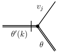
Figure 7: Graphical representation of the interaction vertex $V_{j}$.

The model (50) was considered earlier in Ref. AVH84 in case of the zero-time correlation function

$$\left\langle\phi_{i}(t,{\bm{x}})\phi_{j}(t^{\prime},{\bm{x}^{\prime}})\right\rangle=\delta(t-t^{\prime})\widetilde{D}_{0}\int_{k>m}\frac{d{\bm{k}}}{(2\pi)^{d}}\ P_{ij}({\bm{k}})k^{4-d-y}\ e^{i{\bm{k}\cdot(\bm{x}-\bm{x}^{\prime})}},$$ (55)

where $\widetilde{D}_{0}=D_{0}/\nu_{0}^{2}u_{0}^{2}$. Here, we consider the Navier-Stokes equation (1) with the colored random force (3). As it was shown above the only IR attractive fixed point (39) of this system corresponds to the model with zero-time correlations. This means, that the Galilean symmetry broken by colored noise is restored and we take advantage of the previous study, namely the fact that the full model (50) is multiplicatively renormalizable and possesses the IR attractive fixed point $\left\{g^{*},w^{*}\right\}$ in the full space of couplings

$$g^{*}=\frac{4(d+2)}{3(d-1)}y+O\left(y^{2}\right),\quad w^{*}(w^{*}+1)=\frac{2(d+2)}{d}.$$ (56)

Here, we have introduced the new dimensionless variable $w_{0}=\kappa_{0}/\nu_{0}$ with $\nu_{0}$ from Eq. (1) and its renormalized analog $w$. The critical dimensions of the advected field $\theta$ and additional field $\theta^{\prime}$ are

$$\Delta_{\theta}=-1+y/6,\quad\Delta_{\theta^{\prime}}=d+1-y/6$$ (57)

and have no corrections of the orders $y^{2}$ and higher.

VIII Operator product expansion for the pair correlation function and large-scale anisotropy

Let us consider the influence of the large-scale anisotropy, introduced into the system at the large scale $L$ through the correlation function of the random noise (49), on the inertial range behavior of the pair correlation function $\langle\theta(t,{\bm{x}})\theta(t,{\bm{x}}^{\prime})\rangle$. The goal is to check Kolmogorov’s local symmetry restoration hypothesis, which states that the spatial symmetries of the system are restored in the measurable statistical quantities.

We start our consideration with the structure functions of the following form

$$S_{n}(r)=\langle[\theta(t,{\bm{x}})-\theta(t,{\bm{x}^{\prime}})]^{2n}\rangle.$$ (58)

Dimensionality considerations together with the RG equations give the asymptotic expressions in the region $\mu r\gg 1$:

$$S_{n}(r)=(\nu\mu^{2})^{-n}(\mu r)^{-2n\Delta_{\theta}}\zeta(mr),$$ (59)

where $r=|{\bm{x}^{\prime}}-{\bm{x}}|$, $m=L^{-1}$, the critical dimensions of the fields are given by Eq. (57), and $\zeta$ are certain scaling functions AAV .

We assume that the function $C({\bm{r}}/L_{\theta})$ in Eq. (49) depends additionally on a constant unit vector ${\bm{n}}=\{n_{i}\}$ that determines a certain distinguished direction. Thus, the operator product expansion (OPE) in the irreducible composite operators Zinn

$$[\theta(t,{\bm{x}})-\theta(t,{\bm{x}^{\prime}})]^{2n}\simeq\sum_{F}C_{F}(mr)F(t,{\bm{x}}),\quad{\bm{x}}=({\bm{x}}+{\bm{x}^{\prime}})/2,$$ (60)

which is valid for $r\to 0$, provides the expansion in the irreducible representations of the SO$(d)$ group. Since in order to identify all critical dimensions it is sufficient to consider unaxial anisotropy, Eq. (60) gives rise to the $d$-dimensional generalizations of the Legendre polynomials $P_{l}(\cos\vartheta)$ (which are the basis of such representation), where $\vartheta$ is the angle variable between the vectors ${\bm{r}}$ and ${\bm{n}}$. The structure functions (58) are obtained by averaging (60) with the weight $\exp{\cal S}_{R}$, where ${\cal S}_{R}$ is the renormalized action functional (50). The mean values $\langle F(x)\rangle~{}\propto~{}(mr)^{\Delta_{F}}$ appear in the right hand side.

The main contribution to the “shell” with a given rank $l$ is determined by the $l$th rank operator with the lowest critical dimension. The expansion that takes into account only the leading term in each shell has the form

$$S_{n}\simeq r^{-2n\Delta_{\theta}}\sum_{l=0}^{2n}A_{l}(mr)\,P_{l}(\cos\vartheta)\,(mr)^{\Delta_{(2n,l)}}+\dots,$$ (61)

where we omit the dimensional factors $\nu$ and $\mu$ and the ellipsis stands for the contributions with $l>2n$, which contain more derivatives than fields; $A_{l}(mr)$ are the coefficient functions analytical in $mr$. The dimensions $\Delta_{(2n,l)}$ are the critical dimensions of the operators

$$F^{(n,l)}_{i_{1}\dots i_{l}}=\partial_{i_{1}}\theta\cdots\partial_{i_{l}}\theta\,(\partial_{i}\theta\partial_{i}\theta)^{s}+\dots,$$ (62)

which are constructed solely of the gradients of the passive scalar field and have the lowest canonical dimension (i.e., contain the minimal number of the derivatives). Here, $l$ is the number of the free vector indices (i.e., the rank of the tensor) and $n=l+2s$ is the total number of the fields $\theta$ entering a given operator. The ellipsis then represents the subtractions with Kronecker’s delta symbols that make the operator irreducible (so that the contraction with respect to any pair of the free tensor indices vanishes). For example,

$$F^{(2,2)}_{ij}=\partial_{i}\theta\partial_{j}\theta-\frac{\delta_{ij}}{d}\,(\partial_{k}\theta\partial_{k}\theta).$$ (63)

For the pair correlation functions, the full analog of the expression (61) can be presented in the form that includes all the shells:

$$\langle\theta(t,{\bm{x}})\theta(t,{\bm{x}}^{\prime})\rangle=r^{-2\Delta_{\theta}}\sum_{l=0}^{\infty}A_{l}(mr)\,P_{l}(\cos\vartheta)\,(mr)^{\Delta_{l}}.$$ (64)

This is a consequence of the expression

$$F(x)\partial G(x)=-G(x)\partial F(x)+\partial[F(x)G(x)]$$ (65)

for the operators $F(x)$ and $G(x)$ of the form

$$F_{i_{1}\dots i_{l}}(x)=\theta(x)\partial_{i_{1}}\cdots\partial_{i_{l}}\theta(x)+\dots,$$ (66)

where the ellipsis stands for the subtractions with Kronecker’s delta symbols that make the operator irreducible. It is clear that for the pair correlation function the leading term of the $l$th shell is determined by the single operator (66) with two fields $\theta$ and $l$ tensor indices. From Eq. (65) it follows that this operator is unique up to derivatives, which have vanishing mean values and do not contribute to the quantities of interest; see Secs. IVC and VC in Ref. AK14 for detailed discussion. The critical dimensions $\Delta_{l}$ in Eq. (64) are dimensions of the composite operators (66).

Furthermore, from the relation (65) it follows that for odd $l$ the operator (66) itself reduces to a linear combination of the derivatives. In the following, we will be interested only in the operators which are not reducible to derivatives and will consider only even values of $l$.

IX Inertial range asymptotic behavior of the pair correlation function

In general, a local composite operator is a polynomial constructed from the primary fields $\Phi(x)$ and their finite-order derivatives at a single space-time point $x=\{t,{\bm{x}}\}$. Due to a coincidence of the field arguments, new UV divergences arise in the Green’s functions with such objects Zinn ; Vasiliev . The total canonical dimension of an arbitrary 1-irreducible Green’s function $\Gamma=\langle F\,\Phi\dots\Phi\rangle$ that includes one composite operator $F$ and an arbitrary number of the primary fields $\Phi$ (the formal index of UV divergence) is given by the relation

$$d_{\Gamma}=d_{F}-\sum_{\Phi}N_{\Phi}d_{\Phi},$$ (67)

where $N_{\Phi}$ is the number of the fields $\Phi$ entering $\Gamma$, $d_{\Phi}$ is the total canonical dimension of the given field $\Phi$, $d_{F}$ is the canonical dimension of the operator. In the process of the renormalization operators can mix with each other,

$$F_{i}=\sum_{j}Z_{ij}F_{j}^{R},$$ (68)

where $Z_{ij}$ is the renormalization matrix.

We are interested in the scaling dimensions of the operators (66), which are given by the eigenvalues of the matrix $\Delta_{F}$ [see (45)] calculated for the mixed operators. Since the original stochastic equation (48) is linear in field $\theta$, the necessary diagrams for a calculation of the matrix $Z_{ij}$ do not contain the propagator $\langle\theta\theta\rangle_{0}$ from Eq. (53). Hence, all the calculations can be performed directly in the model without the random noise in Eq. (48), i.e., in the SO$(d)$ covariant model, where the irreducible tensor operators with different ranks cannot mix in renormalization procedure. The only possibility to mix during the renormalization is mixing within the operator’s own “family” of derivatives: the operators with additional derivatives or with the fields $\theta^{\prime}$ and $v_{i}^{\prime}$ have too high canonical dimensions, the appearance of a field $v_{i}$ is forbidden by the (restored) Galilean symmetry, and additional fields $\theta$ are forbidden by the linearity of the model. Herewith, relation (65) shows that all the other operators obtained the same rank differ from (66) by a total derivative and, therefore, give the same contribution into the OPE. This means that the matrix $\Delta_{F}$ is in fact triangular and the composite operators (66) can be treated as multiplicatively renormalizable, $F^{(n,l)}=Z_{(n,l)}F^{(n,l)}_{R}$, with certain renormalization constants $Z_{(n,l)}$ denoted later for simplicity as $Z_{l}$.

Let us introduce $\Gamma_{n}(x;\theta)$, the $\theta^{n}$ term of the expansion in $\theta(x)$ of the generating functional of 1-irreducible Green’s functions with one composite operator $F(x)$ and any number of the fields $\theta$:

$$\Gamma_{n}(x;\theta)=\int dx_{1}\cdots\int dx_{n}\langle F(x)\theta(x_{1})\cdots\theta(x_{n})\rangle\times\theta(x_{1})\cdots\theta(x_{n}).$$ (69)

The renormalization constants $Z_{l}$ are determined by the requirement that the 1-irreducible functions (69) are UV finite in the renormalized theory.

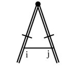
Figure 8: The one-loop approximation of the function $\Gamma_{n}(x;\theta)$. Latin letters $i$ and $j$ denote the internal indices of the velocity field with implied summation.

The one-loop approximation for the 1-irreducible function $\Gamma_{n}(x;\theta)$ can be formally written as

$$\Gamma_{n}(x;\theta)=F(x)+\frac{1}{2}\widetilde{\Delta},$$ (70)

where the first term is the tree (loop-less) approximation, $\widetilde{\Delta}$ is the one-loop graph depicted in Fig. 8, and $1/2$ is the symmetry coefficient of the given graph. The dot with two attached lines in the top of the diagram denotes the operator vertex, i.e., the variational derivative

$$V(x;x_{1},x_{2})=\delta^{2}F(x)/{\delta\theta(x_{1})\delta\theta(x_{2})}.$$ (71)

The contribution of a specific diagram into the functional (70) for any composite operator $F$ is represented in the form

$$\Gamma_{n}=V\times I\times\theta\dots\theta,$$ (72)

where $V$ is the vertex factor given by Eq. (71), $I$ is the diagram itself, and the product $\theta\dots\theta$ corresponds to the external tails.

The calculation of the renormalization constant $Z_{l}$ and anomalous dimension $\gamma_{l}$ (see Appendix B.1 for details) gives

$$Z_{l} = 1-\frac{g}{2(w^{2}+1)}\frac{1}{y}\,{\cal S}_{l}(d),$$ (73)

$$\gamma_{l} = \frac{g}{2(w^{2}+1)}\,{\cal S}_{l}(d).$$ (74)

The factor ${\cal S}_{l}(d)$ in Eqs. (73) and (74) denotes the double sum

$${\cal S}_{l}(d)=\sum_{s,m=0}^{s+m+2\leq l}\frac{(-1)^{s+m}2^{s}C_{l}^{s+m+2}(s+m+2)!}{d(d+2)\dots[d+2(s+m)+2]}\left(\frac{2w^{2}}{w^{2}+1}\right)^{m}.$$ (75)

This sum can be calculated for any given $l$:

$${\cal S}_{l}(d)=\frac{l(l-1)}{4z}\left[\frac{w^{2}+1}{l+z-1}-\frac{w^{2}}{z+1}\,{}_{2}F_{1}\left(1,2-l;2+z;\frac{w^{2}}{w^{2}+1}\right)\right],$$ (76)

where $z=d/2$ and ${}_{2}F_{1}$ is the hypergeomeric function, defined for $|t|<1$ as

$${}_{2}F_{1}(a,b;c;t)=1+\sum_{k=1}^{\infty}\left[\prod_{l=0}^{k-1}\frac{(a+l)(b+l)}{(1+l)(c+l)}\right]\,t^{k};$$ (77)

see Appendix B.2 for details.

The critical dimension of the operator (66) is obtained using the relations (45) and (57)

$$\Delta_{l}=l+2\Delta_{\theta}+\gamma_{l}^{*}=l-2+y/3+\gamma_{l}^{*},$$ (78)

where $\gamma_{l}^{*}$ is the value of $\gamma_{l}$ at the fixed point. For the realistic values of the parameters $d=3$ and $w^{*}\approx 1.393$, see Eq. (56), we get

$$\gamma_{l}^{*}\approx 0.566\,{\cal S}_{l}(3/2)\times y$$ (79)

with the higher-order corrections in scaling exponent $y$. The factor ${\cal S}_{l}(3/2)$ is given by the expression

$${\cal S}_{l}(3/2)=\frac{l(l-1)}{6}\,\left[\frac{2.94}{l+1/2}-0.776\,{}_{2}F_{1}\left(1,2-l;7/2;0.66\right)\right]$$ (80)

and depends on $l$ as depicted in Fig. 9; the same type of behavior is valid for any spatial dimension $d\geq 3$.

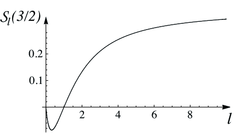
Figure 9: The graph of the function ${\cal S}_{l}(3/2)$ as a function of $l$.

It is important that ${\cal S}_{l}(3/2)>0$ for $l\geq 1$: this leads to a monotonical increase of $\Delta_{l}$ as $l\to\infty$, see expression (78). Moreover, $\Delta_{0}<0$. The quantity of the spatial derivatives $l$ illustrate the degree of anisotropy: the larger $l$ the higher the degree of the anisotropy, see Eq. (64). Thus, there is a hierarchy of the anisotropic contributions in the inertial range asymptotic behavior of the pair correlation function (64), and the leading term is given by the scalar operator $\theta^{2}$.

This fact has a clear physical interpretation: in the inertial range, the leading contribution is given by the isotropic shell $l=0$ and coincides with the scalar isotropic model, while the terms with $l\geq 2$ provide only corrections which become insignificant as $mr\to 0$. Moreover, the corrections become less pronounced with increasing $l$, i.e., with increasing degree of the anisotropy. This effect confirms Kolmogorov’s hypothesis of the local isotropy restoration.

It is worth mentioning that same analogy exists between the present hierarchy and the well-known multipole expansion in ordinary classical electrostatics which can also be written as an expansion in spherical harmonics Jackson . The multipole expansion can be viewed as a series with progressively finer angular features. The initial isotropic term, corresponding to the potential of a point-like charge, gives the leading contribution at large distances. The other terms are anisotropic (they involve angular dependence) and give corrections that decay faster and faster as the “degree of anisotropy” $l$ increases.

This is not just a superficial analogy. It becomes especially clear if one applies the zero-mode approach to the advection problem in the Kraicnan’s rapid-change model (or in some analogous model, in which turbulent flow is simulated by some Gaussian statistics); see, e.g., Ref. LM . Employing the zero-mode approach terminology, the individual terms of the spherical harmonics expansion in electrostatics are the homogeneous solutions (the so-called zero modes) of the Poisson equation. If we are interested in the asymptotic behavior at small or large distances, only the zero modes restricted at the origin or at infinity should be taken into account, respectively. The difference with electrostatic problems is that for the turbulent advection the differential operator is more complicated. Moreover, since we are interested in the inertial range behavior (i.e., behavior in the interval, restricted by both large and small scales) it is not so simple to choose the right solution from two possible zero modes. Nevertheless, the result is similar to the electrostatic case: the leading term corresponds to $l=0$ and is isotropic, while the other (anisotropic) contributions provide the decaying corrections and obey the hierarchy with respect to the value of $l$.

X Conclusion

In this paper incompressible fluid is studied using the field theoretic approach. We have considered the stochastic Navier-Stokes equation with colored noise (i.e., the model with arbitrary finite correlation time of the velocity field) to describe fluid dynamics. The second problem considered is the advection of the passive scalar field by this turbulent flow. The critical dimensions of the fields are calculated for both problems.

Within the one-loop approximation the only nontrivial regime of the long-distance (IR) behavior is found to be reduced to the limiting case of the rapid-change type behavior. This regime is realized for $y>0$, $\eta>y/3$, where $y$ and $\eta$ describe the energy spectrum ${\cal E}\propto k^{1-y}$ and the dispersion law $\omega\sim k^{2-\eta}$ of the velocity field. The second nontrivial fixed point, existing if $\frac{1}{3}<\frac{y}{\eta}<\frac{1}{3}+\frac{4/3}{3d(d-1)+2}$, is a saddle type point. The fact that the only nontrivial IR attractive fixed point corresponds to vanishing correlation time means, in particular, that the Galilean symmetry, violated by the colored stochastic force, is automatically restored in the IR limit. As it should be for the case of rapid-change behavior, the calculated critical dimensions of the fields coincide with the results obtained for the zero-time model which was considered earlier in Ref. NS-Zero .

The inertial-range behavior of the correlation function of two composite operators constructed from the advected fields $\theta$ was studied using the OPE. Existence of the anomalous scaling (singular power-like dependence on the integral scale $L$) was established. From the leading-order (one-loop) calculations it follows that the main contribution into the OPE is given by the isotropic term corresponding to $l=0$, where $l$ is the number of the Legendre polynomial entering the expansion of the correlation function and signifies a degree of the anisotropy; all other terms with $l\geq 2$ provide only corrections.

These two facts (the restoration of the Galilean symmetry and isotropy restoration) give a quantitative illustration of the general concept that the symmetries of the Navier–Stokes equation, broken spontaneously and by initial or boundary conditions, are restored in the statistical sense for fully developed turbulence Legacy ; LegacyD ; Monin ; K41a ; K41b ; K41c .

Appendix A Calculation details for the model of incompressible fluid

This section contains detailed calculations of the diagrams, defining the renormalization constants $Z_{1}$ and $Z_{2}$ (see Sec. IV). All calculations are performed in the analytical regularization and MS scheme.

A.1 Calculation of the self-energy operator

Let us start with the graph presented in Fig. 3. The analytical expression for it reads

$$\Sigma_{\alpha\beta} = D_{0}\int\frac{d\omega}{2\pi}\int\frac{d{\bm{k}}}{(2\pi)^{d}}V_{\alpha ab}({\bm{p}})V_{dc\beta}({\bm{p}+\bm{k}})P_{ac}({\bm{p}+\bm{k}})P_{bd}({\bm{k}})$$ (81)

$$\times \frac{k^{8-d-y-2\eta}}{(\omega^{2}+\nu_{0}^{2}u_{0}^{2}k^{4-2\eta})(\omega^{2}+\nu_{0}^{2}k^{4})(-i\omega+\nu_{0}|{\bm{p}+\bm{k}}|^{2})}.$$

Here and below $V_{ijk}({\bm{p}})$ is the triple vertex (10); Greek letters $\alpha$, $\beta$ and Latin letters $a$ – $d$ denote the vector indices of the propagators (8) and (9) with the implied summation over the repeated indices. Since the index of divergence for this diagram $d_{\Gamma}=2$, we have to calculate only the terms proportional to $p^{2}$, where $\bm{p}$ denotes an external momentum.

Let us consider the expression (19). Taking trace of both sides of it one obtains the scalar equation

$$\Gamma_{2}=i\omega-\nu_{0}p^{2}+\Sigma,$$ (82)

where we have introduced for brevity

$$\Sigma=\Sigma_{\alpha\beta}P_{\alpha\beta}/(d-1).$$ (83)

The calculation of the (scalar) index structure $J$ of the quantity $\Sigma$ yields

$$J = V_{\alpha ab}({\bm{p}})V_{dc\beta}({\bm{p}+\bm{k}})P_{ac}({\bm{p}+\bm{k}})P_{bd}({\bm{k}})P_{\alpha\beta}({\bm{p}})$$

$$\cong ({\bm{A}\cdot\bm{p}})+Bp^{2}+{\it O}({p}^{3}).$$

The vector coefficient ${\bm{A}}$ and scalar coefficient $B$ are

$${\bm{A}} = 2{\bm{k}},$$ (85)

$$B = \sin^{4}\varphi-3\sin^{2}\varphi\cos^{2}\varphi+(2-d)\sin^{2}\varphi,$$ (86)

where $\varphi$ is the angle between the external momenta ${\bm{p}}$ and internal momenta ${\bm{k}}$.

The integration over the frequency $\omega$ in the expression (81) gives

$$\int\frac{d\omega}{2\pi}\frac{1}{(\omega^{2}+\nu_{0}^{2}u_{0}^{2}k^{4-2\eta})(\omega^{2}+\nu_{0}^{2}k^{4})(-i\omega+\nu_{0}|{\bm{p}+\bm{k}}|^{2})}$$

$$=\frac{1}{2\nu_{0}^{4}}\frac{u_{0}k^{2-\eta}+k^{2}+|{\bm{p}+\bm{k}}|^{2}}{u_{0}k^{2}k^{2-\eta}(k^{2}+u_{0}k^{2-\eta})(u_{0}k^{2-\eta}+|{\bm{p}+\bm{k}}|^{2})(k^{2}+|{\bm{p}+\bm{k}}|^{2})}.$$ (87)

Combining the expression (A.1) with the numerator of the expression (A.1) gives

$$\Sigma\propto\int\frac{d{\bm{k}}}{(2\pi)^{d}}\frac{\widehat{{\bm{A}}}+\widehat{{\bm{B}}}}{u_{0}k^{4-\eta}(k^{2}+u_{0}k^{2-\eta})(u_{0}k^{2-\eta}+|{\bm{p}+\bm{k}}|^{2})(k^{2}+|{\bm{p}+\bm{k}}|^{2})}.$$ (88)

Here, the coefficients $\widehat{{\bm{A}}}$ and $\widehat{{\bm{B}}}$ denote the quantities proportional to $p^{2}$ and $\bm{p}$, respectively:

$$\widehat{{\bm{A}}} = p^{2}(u_{0}k^{2-\eta}+2k^{2}){\bm{A}}+2B({\bm{p}\cdot\bm{k}}){\bm{p}},$$ (89)

$$\widehat{{\bm{B}}} = B(u_{0}k^{2-\eta}+2k^{2}){\bm{p}},$$ (90)

with the vector ${\bm{A}}$ and scalar $B$ defined in the expressions (85) and (86).

The integration over the internal momenta ${\bm{k}}$ can be simplified in the MS scheme, in which all the anomalous dimensions $\gamma_{1,2}$ are independent of the regularizers like $y$ and $\eta$. Hence, we may choose them arbitrarily with the only restriction that our diagrams have to remain UV finite; see Ref. FinTimeEta for detailed discussion. The most convenient way is to put $\eta=0$, so expanding the denominator of (88), combining it with (89) – (90) and taking into account that we are interested only in the term proportional to ${\bm{p}}$ for $\widehat{{\bm{B}}}$ and to $p^{0}$ for $\widehat{{\bm{A}}}$ one obtains

$$\Sigma_{\alpha\beta}\propto p^{2}\frac{1}{2(u_{0}+1)}\int\frac{d{\bm{k}}}{(2\pi)^{d}}\frac{1}{k^{2}}\biggl{[}A(u_{0}+2)-4\sin^{2}\varphi\cos^{2}\varphi+\frac{2(u_{0}+2)(u_{0}+3)}{u_{0}+1}\sin^{2}\varphi\cos^{2}\varphi\biggr{]};$$ (91)

the coefficient $A$ is defined in Eq. (85).

In order to integrate over the vector ${\bm{k}}$ we need to average the expression (91) over the angles:

$$\int d{\bm{k}}f({\bm{k}})=S_{d}\int_{m}^{\infty}dk\,k^{d-1}\,\left\langle f({\bm{k}})\right\rangle,$$ (92)

where $\langle\cdots\rangle$ is the averaging over the unit sphere in the $d$-dimensional space, $S_{d}$ is its surface area, and $k=|{\bm{k}}|$. To average the function (91) over the angles in the orthogonal subspace we use the relations

$$\left\langle\cos^{2}\varphi\right\rangle = \frac{1}{d},$$ (93)

$$\left\langle\cos^{4}\varphi\right\rangle = \frac{3}{d(d+2)}.$$

This gives

$$\Sigma\propto p^{2}\frac{2}{(u_{0}+1)^{2}}\int\frac{d{\bm{k}}}{(2\pi)^{d}}\frac{1}{k^{2}}X,$$ (94)

where

$$X=\frac{d-1}{d(d+2)}\left[u_{0}^{2}d(d-1)+3u_{0}d(d-1)+2d^{2}-2d+4\right].$$ (95)

Combining the expression (81) with the expressions (83), (A.1), (94), and expression (4) for the amplitude $D_{0}$ we find

$$\Sigma_{\alpha\beta}=-\frac{1}{4}p^{2}g_{0}\nu_{0}\frac{u_{0}}{(u_{0}+1)^{3}}X\int_{m}^{\infty}\frac{dk}{(2\pi)^{d}}\frac{1}{k^{d+y}}.$$ (96)

Taking into account the multiplier $(d-1)^{-1}$ coming from (83), after the integration of the expression (96) over the modulus $k$ one obtains

$$\Sigma=-\frac{1}{4}p^{2}g_{0}\nu_{0}\frac{u_{0}^{3}d(d-1)+3u_{0}^{2}d(d-1)+2u_{0}(d^{2}-d+2)}{d(d+2)(u_{0}+1)^{3}}C_{d}\frac{m^{-y}}{y},$$ (97)

where $C_{d}\equiv S_{d}/(2\pi)^{d}$. Combining this expression with Eq. (19) from Sec. IV one immediately obtains the renormalization constant $Z_{2}=Z_{\nu}$.

A.2 Calculation of the vertex diagrams

Let us start with the graph presented in Fig. 4a. The analytical expression for it is

$$\Delta_{1} = D_{0}\int\frac{d\omega}{2\pi}\int\frac{d{\bm{k}}}{(2\pi)^{d}}V_{\alpha cd}({\bm{p}})V_{a\beta b}(-\bm{k})V_{ef\gamma}({\bm{p}+\bm{k}})$$

$$\times \frac{P_{ac}(\bm{k})P_{de}({\bm{p}+\bm{k}})P_{bf}({\bm{q}-\bm{k}})}{(i\omega+\nu_{0}k^{2})(-i\omega+\nu_{0}|{\bm{p}+\bm{k}}|^{2})}\frac{(q-k)^{8-d-y-2\eta}}{(\omega^{2}+\nu_{0}^{2}|\bm{q}-\bm{k}|^{4})(\omega^{2}+\nu_{0}^{2}u_{0}^{2}|\bm{q}-\bm{k}|^{4-2\eta})}.$$

Here and below $\bm{p}$ and $\bm{q}$ are the external momenta, $\bm{k}$ denotes an internal (loop) momenta; the index of divergence for this diagram $d_{\Gamma}=1$, therefore, we need to calculate only the terms, proportional to ${\bm{p}}^{1}$ or ${\bm{q}}^{1}$. Since $\Delta_{1}\propto V_{\alpha cd}({\bm{p}})$, we may set $q=p=0$ in all the other multipliers. This observation significantly simplifies the expression for the divergent part of Eq. (A.2)

$$\Delta_{1} \cong D_{0}\int\frac{d\omega}{2\pi}\int\frac{d{\bm{k}}}{(2\pi)^{d}}V_{\alpha cd}({\bm{p}})V_{a\beta b}(-\bm{k})V_{ef\gamma}({\bm{k}})$$

$$\times \frac{P_{ac}(\bm{k})P_{de}({\bm{k}})P_{bf}({\bm{k}})}{(i\omega+\nu_{0}{k}^{2})(-i\omega+\nu_{0}k^{2})}\frac{k^{8-d-y-2\eta}}{(\omega^{2}+\nu_{0}^{2}k^{4})(\omega^{2}+\nu_{0}^{2}u_{0}^{2}k^{4-2\eta})}.$$

Integration over the frequency at $\eta=0$ leads to

$$\int\frac{d\omega}{2\pi}\frac{1}{(i\omega+\nu_{0}{k}^{2})(-i\omega+\nu_{0}k^{2})(\omega^{2}+\nu_{0}^{2}k^{4})(\omega^{2}+\nu_{0}^{2}u_{0}^{2}k^{4-2\eta})}=\frac{u_{0}+2}{4k^{10}\nu_{0}^{5}u_{0}(u_{0}+1)^{2}}.$$ (100)

The calculation of the index structure $J^{1}_{\alpha\beta\gamma}$ of the quantity $\Delta_{1}$ is straighforward

$$J^{1}_{\alpha\beta\gamma} = V_{\alpha cd}({\bm{p}})V_{a\beta b}(-\bm{k})V_{ef\gamma}({\bm{k}})P_{ac}(\bm{k})P_{de}({\bm{k}})P_{bf}({\bm{k}})$$

$$= 2i\left[p_{\alpha}-\frac{(\bm{p}\cdot\bm{k})k_{\alpha}}{k^{2}}\right]k_{\beta}k_{\gamma}.$$

In order to integrate the expression (A.2) over the vector $\bm{k}$ we employ the relations similar to Eqs. (93)

$$\left\langle\frac{k_{i}k_{j}}{k^{2}}\right\rangle = \frac{\delta_{ij}}{d},$$ (102)

$$\left\langle\frac{k_{i}k_{j}k_{l}k_{m}}{k^{4}}\right\rangle = \frac{\delta_{ij}\delta_{lm}+\delta_{il}\delta_{jm}+\delta_{im}\delta_{jl}}{d(d+2)}.$$

Taking into account the expressions (100) – (102), for the divergent part of the diagram $\Delta_{1}$ one obtains

$$\Delta_{1}=i\,g_{0}\frac{u_{0}(u_{0}+2)}{2(u_{0}+1)^{2}}\frac{(d+1)p_{\alpha}\delta_{\beta\gamma}-p_{\beta}\delta_{\alpha\gamma}-p_{\gamma}\delta_{\alpha\beta}}{d(d+2)}C_{d}\frac{m^{-y}}{y}.$$ (103)

The analytical expression for the graph presented in Fig. 4b is

$$\Delta_{2} = D_{0}\int\frac{d\omega}{2\pi}\int\frac{d{\bm{k}}}{(2\pi)^{d}}V_{\alpha cd}({\bm{p}})V_{a\beta b}(\bm{p}-\bm{k})V_{fe\gamma}({\bm{q}-\bm{k}})$$

$$\times \frac{P_{ac}(\bm{p}-\bm{k})P_{de}({\bm{k}})P_{bf}({\bm{q}-\bm{k}})}{(i\omega+\nu_{0}|\bm{p}-{\bm{k}}|^{2})(i\omega+\nu_{0}|{\bm{q}-\bm{k}}|^{2})}\frac{k^{8-d-y-2\eta}}{(\omega^{2}+\nu_{0}^{2}k^{4})(\omega^{2}+\nu_{0}^{2}u_{0}^{2}k^{4-2\eta})}.$$

Like in the previous case, since $\Delta_{2}\propto V_{\alpha cd}({\bm{p}})$ we may set $q=p=0$ in all the other multipliers:

$$\Delta_{2} \cong D_{0}\int\frac{d\omega}{2\pi}\int\frac{d{\bm{k}}}{(2\pi)^{d}}V_{\alpha cd}({\bm{p}})V_{a\beta b}(\bm{k})V_{fe\gamma}({\bm{k}})$$

$$\times \frac{P_{ac}(\bm{k})P_{de}({\bm{k}})P_{bf}({\bm{k}})}{(i\omega+\nu_{0}k^{2})^{2}}\frac{k^{8-d-y-2\eta}}{(\omega^{2}+\nu_{0}^{2}k^{4})(\omega^{2}+\nu_{0}^{2}u_{0}^{2}k^{4-2\eta})}.$$

The integration over the frequency $\omega$ at $\eta=0$ leads to the expression

$$\int\frac{d\omega}{2\pi}\frac{1}{(i\omega+\nu_{0}{k}^{2})^{2}(\omega^{2}+\nu_{0}^{2}k^{4})(\omega^{2}+\nu_{0}^{2}u_{0}^{2}k^{4-2\eta})}=\frac{u_{0}(u_{0}+3)+4}{8k^{10}\nu_{0}^{5}u_{0}(u_{0}+1)^{3}}.$$ (106)

The calculation of the index structure $J^{2}_{\alpha\beta\gamma}$ gives

$$J^{2}_{\alpha\beta\gamma} = V_{\alpha cd}({\bm{p}})V_{a\beta b}(\bm{k})V_{fe\gamma}({\bm{k}})P_{ac}(\bm{k})P_{de}({\bm{k}})P_{bf}({\bm{k}})$$

$$= -2ip_{c}P_{c\alpha}(\bm{k})k_{\beta}k_{\gamma}.$$

Taking into account the expressions (106) and (A.2), the integration of the expression (A.2) over the momenta $\bm{k}$ gives

$$\Delta_{2}=-i\,g_{0}\frac{u_{0}(u_{0}^{2}+3u_{0}+4)}{4(u_{0}+1)^{3}}\frac{(d+1)p_{\alpha}\delta_{\beta\gamma}-p_{\beta}\delta_{\alpha\gamma}-p_{\gamma}\delta_{\alpha\beta}}{d(d+2)}C_{d}\frac{m^{-y}}{y}.$$ (108)

The analytical expression for the divergent part of the graph presented in Fig. 4c coincides with the expression (A.2). Thus, $\Delta_{3}=\Delta_{2}$ and it is also given by the expression (108).

Using the transversality condition $\partial_{i}v_{i}=0$ together with the expression (10) and moving the derivative in the vertex from the field ${\bm{v}}^{\prime}$ onto the field ${\bm{v}}$ we conclude that the term proportional to a momentum $p_{\alpha}$ gives no contribution, therefore for the sum of the three triangle diagrams $\Delta_{1}$, $\Delta_{2}$, and $\Delta_{3}$ [see Eqs. (103) and (108)] one obtains

$$\Delta_{1}+\Delta_{2}+\Delta_{3}=i\,g_{0}\frac{u_{0}}{(u_{0}+1)^{3}}\frac{p_{\beta}\delta_{\alpha\gamma}+p_{\gamma}\delta_{\alpha\beta}}{d(d+2)}C_{d}\frac{m^{-y}}{y}.$$ (109)

Combining this expression with Eq. (20) from Sec. IV one immediately obtains the renormalization constant $Z_{1}=Z_{v}$.

Appendix B Calculation details for the model of passive advection

This section contains detailed calculations of the diagram, defining the renormalization constant $Z_{l}$, and the double sum ${\cal S}_{l}(d)$, entering in the expression for the anomalous dimension $\gamma_{l}$ (see Sec. IX). The calculation of renormalization constant is performed in the analytical regularization and the MS scheme.

B.1 Calculation of the diagram with insertion of the composite operator

The only graph $\widetilde{\Delta}$ which is required for the critical dimensions of the correlation functions (64) is presented in Fig. 8. To simplify the process of calculations it is convenient to contract the operator (66) with a constant vector ${\bm{\lambda}}=\{\lambda_{i}\}$. As a result one obtains the scalar operator

$$F_{l}=\theta(\lambda_{i}\partial_{i})^{l}\theta+\dots,$$ (110)

where the terms, denoted by the ellipsis, necessarily involve the factors of $\lambda^{2}$. The appearance of $\lambda^{2}$ means that the corresponding initial operator contains $\partial^{2}$, i.e., its canonical dimension is too high. Therefore, we should omit the terms with $\lambda^{2}$. The vertex factor (71) in this case takes the form

$$V(x;x_{1},x_{2})=\delta(x-x_{1})(\lambda_{i}\partial_{i})^{l}\delta(x-x_{2})+\{x_{1}\leftrightarrow x_{2}\}.$$ (111)

Let us choose the external momentum ${\bm{p}}$ to flow into the diagram through the left lower vertex and to flow out of the diagram through the right lower one. Since the divergence of the graph $\widetilde{\Delta}$ is logarithmic, the external momentum flowing through the operator vertex and all the external frequencies are set equal to zero. We are interested in the value of the anomalous dimension at the fixed point, therefore, we may perform the substitutions $g=g^{*}$, $w=w^{*}$ [see Eq. (56)] and $u\to\infty$ from the very beginning; furthermore, the limiting case $u\to\infty$ means that $(u_{0}\nu_{0})^{2}\gg\omega^{2}$, so the propagator function (8) reads

$$\left\langle v_{i}v_{j}\right\rangle_{0}=g_{0}\nu_{0}^{3}\ \frac{k^{4-d-y}}{\omega^{2}+\nu_{0}^{2}k^{4}}P_{ij}({\bm{k}}).$$ (112)

Thus, the core of the diagram takes the form

$$\widetilde{\Delta}\cong p_{i}p_{j}\,\int\frac{d\omega}{2\pi}\int_{k>m}\frac{d{\bm{k}}}{(2\pi)^{d}}\,2i^{l}({\bm{\lambda}}\cdot{\bm{q}})^{l}\,\frac{g\mu^{y}\nu^{3}k^{4-d-y}}{\omega^{2}+\nu^{2}k^{4}}\,P_{ij}({\bm{k}})\,\frac{1}{\omega^{2}+w^{2}\nu^{2}q^{4}}.$$ (113)

Here the factor $p_{i}p_{j}$ comes from the vertices $V_{j}$ [see Eq. (54)] and from the observation that in the case of incompressible carrying fluid the derivative can act directly on the field $\theta$; the factor $2i^{l}({\bm{\lambda}}\cdot{\bm{q}})^{l}$ comes from the vertex (111) for even $l$ (for odd $l$ the two terms in Eq. (111) would cancel each other), the factors depending on ${\bm{k}}$ represent the velocity correlation function (112), the last factor comes from the propagators $\langle\theta^{\prime}\theta\rangle_{0}$; the momentum ${\bm{k}}$ flows through the velocity propagator, so that ${\bm{q}}={\bm{k}}+{\bm{p}}$.

In order to find the corresponding renormalization constant it is sufficient to retain in the result for the counterterm only the terms of the same form, i.e., the terms of the form $({\bm{\lambda}}\cdot{\bm{p}})^{l}$, and drop all the other terms containing $\lambda^{2}$ or $p^{2}$. Thus, the structure with $P_{ij}({\bm{k}})$ is simplified and takes the form

$$p_{i}p_{j}P_{ij}({\bm{k}})\cong-({\bm{p}\cdot\bm{k}})^{2}/k^{2}.$$ (114)

The integration over the frequency $\omega$ in Eq. (113) is straightforward

$$\widetilde{\Delta}\cong-g\mu^{y}\,i^{l}\int_{k>m}\frac{d{\bm{k}}}{(2\pi)^{d}}\,({\bm{p}\cdot\bm{k}})^{2}(\bm{\lambda}\cdot{\bm{q}})^{l}\,\frac{k^{-d-y}}{q^{2}(k^{2}+w^{2}q^{2})}.$$ (115)

Expanding all the denominators in the integrand of Eq. (115) in ${\bm{p}}$ together with dropping all the terms with $p^{2}$ gives

$$\frac{1}{q^{2}}\simeq\frac{1}{k^{2}+2({\bm{p}\cdot\bm{k}})}=\frac{1}{k^{2}}\sum^{\infty}_{s=0}\frac{(-2)^{s}({\bm{p}\cdot\bm{k}})^{s}}{k^{2s}};$$ (116)

$$\frac{1}{k^{2}+w^{2}q^{2}} \simeq \frac{1}{k^{2}(w^{2}+1)+2w^{2}({\bm{p}\cdot\bm{k}})}=\frac{1}{(w^{2}+1)k^{2}}\sum_{m=0}^{\infty}\frac{(-1)^{m}({\bm{p}\cdot\bm{k}})^{m}}{k^{2m}}\left(\frac{2w^{2}}{w^{2}+1}\right)^{m}.$$ (117)

Expanding the numerator of (115) using Newton’s binomial formula (note, that ${\bm{q}}={\bm{k}}+{\bm{p}}$) one obtains

$$({\bm{\lambda}}\cdot{\bm{q}})^{l}=\sum_{n=0}^{l}C_{l}^{n}({\bm{\lambda}}\cdot{\bm{k}})^{n}({\bm{\lambda}}\cdot{\bm{p}})^{l-n}.$$ (118)

Combining the expressions (116) – (118) one obtains threefold series over $n,m$, and $s$:

$$(\bm{\lambda}\cdot{\bm{q}})^{l}\,\frac{1}{q^{2}(k^{2}+w^{2}q^{2})}=\frac{1}{k^{4}(w^{2}+1)}\sum_{n=0}^{l}C_{l}^{n}({\mbox{\boldmath$\lambda$}}\cdot{\bm{p}})^{l-n}\sum_{m,s=0}^{\infty}\frac{(-1)^{m}(-2)^{s}({\bm{p}\cdot\bm{k}})^{m+s+2}({\mbox{\boldmath$\lambda$}}\cdot{\bm{k}})^{n}}{k^{2(s+m)}}\left(\frac{2w^{2}}{w^{2}+1}\right)^{m},$$ (119)

in which we need to collect only the terms proportional to $({\mbox{\boldmath$\lambda$}}\cdot{\bm{p}})^{l}$. This leads to the restriction $n=s+m+2$ and hence to the finite double sum

$$(\bm{\lambda}\cdot{\bm{q}})^{l}\,\frac{1}{q^{2}(k^{2}+w^{2}q^{2})} \cong \frac{1}{k^{4}(w^{2}+1)}$$

$$\times \sum_{s,m=0}^{s+m+2\leq l}(-1)^{m}(-2)^{s}C_{l}^{s+m+2}\frac{({\mbox{\boldmath$\lambda$}}\cdot{\bm{p}})^{l-m-s-2}({\bm{p}\cdot\bm{k}})^{m+s+2}({\mbox{\boldmath$\lambda$}}\cdot{\bm{k}})^{s+m+2}}{k^{2(s+m)}}\left(\frac{2w^{2}}{w^{2}+1}\right)^{m}.$$

Substitution of this sum into the expression (115) gives rise to the integrals

$$I_{i_{1}\dots i_{2n}}(m)=\int_{k>m}\frac{d{\bm{k}}}{(2\pi)^{d}}\,k^{-d-y}\,\frac{k_{i_{1}}\dots k_{i_{2n}}}{k^{2n}}$$ (121)

with $n=s+m+2\geq 2$. They can be found using the expressions

$$I_{i_{1}\dots i_{2n}}(m)=\frac{\delta_{i_{1}i_{2}}\dots\delta_{i_{2n-1}i_{2n}}+{\rm all\ permutations}}{d(d+2)\dots(d+2n-2)}\,I(m),$$ (122)

where $I(m)$ is the scalar integral

$$I(m)=\int_{k>m}\frac{d{\bm{k}}}{(2\pi)^{d}}\frac{1}{k^{d+y}}=C_{d}\frac{m^{-y}}{y}.$$ (123)

The sum over all the possible permutations of $2n$ tensor indices in the numerator of Eq. (122) involves $(2n-1)!!=(2n)!/2^{n}n!$ terms, but we have to keep only the terms that give rise to the structure $({\mbox{\boldmath$\lambda$}}\cdot{\bm{p}})^{n}$ after the contraction with the vectors $\lambda$ and ${\bm{p}}$ in the expression (B.1). Hence, there are only $n!$ such permutations.

Collecting all the factors for the core (113) leads to the expression

$$\widetilde{\Delta}\cong-i^{l}({\mbox{\boldmath$\lambda$}}\cdot{\bm{p}})^{l}g\frac{1}{(w^{2}+1)}C_{d}\left(\frac{\mu}{m}\right)^{y}\frac{1}{y}{\cal S}_{l}(d),$$ (124)

where

$${\cal S}_{l}(d)=\sum_{s,m=0}^{s+m+2\leq l}\frac{(-1)^{s+m}2^{s}C_{l}^{s+m+2}(s+m+2)!}{d(d+2)\dots[d+2(s+m)+2]}\left(\frac{2w^{2}}{w^{2}+1}\right)^{m}.$$ (125)

For $l=0$, sums (B.1) and (125) contain no terms, so that ${\cal S}_{0}(d)=0$.

Thus, expression (70) for the functional (69) reads

$$\Gamma_{2}(x)=F_{l}(x)\left[1-\frac{g}{2(w^{2}+1)}\left(\frac{\mu}{m}\right)^{y}\frac{1}{y}\,{\cal S}_{l}(d)\right],$$ (126)

where $F_{l}$ is the operator (110) and the substitution $g\to gC_{d}$ is implied. For the renormalization constant $Z_{l}$ in the MS scheme one obtains

$$Z_{l}=1-\frac{g}{2(w^{2}+1)}\frac{1}{y}\,{\cal S}_{l}(d).$$ (127)

Accordingly to Sec. VIII the parameter $l$ defining the composite operator (110) counts the Legendre polynomials entering in the OPE for correlation functions.

B.2 Calculation of the double sum ${\cal S}_{l}(d)$

It turns out that the double sum ${\cal S}_{l}(d)$ in Eqs. (75) and (125) can be reduced to a simpler onefold sum. Let us pass from the set of variables $s$ and $m$ to the new summation variables $k$ and $m$, where $k=s+m$, and substitute the explicit expression for the binomial coefficient $C^{k+2}_{l}=l!/(k+2)!(l-k-2)!$. This gives

$${\cal S}_{l}(d)=l!\sum_{k=0}^{k+2\leq l}\left[\sum_{m=0}^{k}\left(\frac{w^{2}}{w^{2}+1}\right)^{m}\right]\,\frac{(-2)^{k}}{(l-k-2)!\,d(d+2)\dots(d+2k+2)}.$$ (128)

The internal summation over $m$ gives

$$\sum_{m=0}^{k}\left(\frac{w^{2}}{w^{2}+1}\right)^{m}=(w^{2}+1)\left[1-\left(\frac{w^{2}}{w^{2}+1}\right)^{k+1}\right];$$ (129)

changing now the summation variable $k\to k+2$ one obtains

$${\cal S}_{l}(d)=l!\,(w^{2}+1)\sum_{k=2}^{l}\frac{(-2)^{k-2}}{(l-k)!\,d(d+2)\dots(d+2k-2)}\left[1-\left(\frac{w^{2}}{w^{2}+1}\right)^{k-1}\right].$$ (130)

Substitution $z=d/2$ allows us to construct the expression with the ratio of two factorials

$${\cal S}_{l}(z)=l!\,(w^{2}+1)\sum_{k=2}^{l}\frac{(-1)^{k}(z-1)!}{4(l-k)!\,(z+k-1)!}\left[1-\left(\frac{w^{2}}{w^{2}+1}\right)^{k-1}\right],$$ (131)

which can be calculated for any given $l$:

$${\cal S}_{l}(z)=\frac{l(l-1)}{4z}\left[\frac{w^{2}+1}{l+z-1}-\frac{w^{2}}{z+1}\,{}_{2}F_{1}\left(1,2-l;2+z;\frac{w^{2}}{w^{2}+1}\right)\right].$$ (132)

Here ${}_{2}F_{1}$ denotes the hypergeomeric function, defined for $|t|<1$ as

$${}_{2}F_{1}(a,b;c;t)=1+\sum_{k=1}^{\infty}\left[\prod_{l=0}^{k-1}\frac{(a+l)(b+l)}{(1+l)(c+l)}\right]\,t^{k}.$$ (133)

The explicit expression (132) allows us to analyze the dependence of the anomalous dimensions $\gamma_{l}$ over $l$ being in the present context the degree of the anisotropy.

References

References

- (1) U. Frisch, Turbulence: The Legacy of A.N. Kolmogorov (Cambridge University Press, Cambridge, 1995).
- (2) P. A. Davidson, Turbulence. An introduction for Scientists and Engineers (Oxford University Press, Oxford, 2005).
- (3) A. S. Monin and A. M. Yaglom, Statistical fluid mechanics, vol. 2 (MIT Press, Cambridge, 1975).
-
(4)
A. N. Kolmogorov, Dokl. Akad. Nauk SSSR 30(4), 299 (1941);
reprinted in Proc. R. Soc. Lond. A 434, 9 (1991). - (5) A. N. Kolmogorov, Dokl. Akad. Nauk SSSR 31(6), 538 (1941).
-
(6)
A. N. Kolmogorov, Dokl. Akad. Nauk SSSR 32(1), 19 (1941);
reprinted in Proc. R. Soc. Lond. A 434, 15 (1991). - (7) L. F. Richardson, Weather Prediction by Numerical Process (Cambridge University Press, Cambridge, 1922).
- (8) H. Effinger and S. Grossmann, Phys. Rev. Lett. 53, 442 (1984).
- (9) K. R. Sreenivasan and R. A. Antonia, Annu Rev. Fluid. Mech. 29, 435 (1997).
- (10) I. Arad, B. Dhruva, S. Kurien, V. L’vov, I. Procaccia, and K. R. Sreenivasan, Phys. Rev. Lett. 81, 5330 (1998).
- (11) V. Borue and S. A. Orszag, J. Fluid Mech. 306, 293 (1996).
- (12) I. Arad, V. L’vov, and I. Procaccia, Phys. Rev. E 59, 6753 (1999).
- (13) I. Arad, L. Biferale, and I. Procaccia, Phys. Rev. E 61, 2654 (2000).
- (14) L. Biferale and I. Procaccia, Phys. Rep. 414, 43 (2005).
- (15) G. Falkovich, K. Gawȩdzki, and M. Vergassola, Rev. Mod. Phys. 73, 913 (2001).
- (16) J. Zinn-Justin, Quantum Field Theory and Critical Phenomena, 4th ed. (Oxford University Press, Oxford, 2002).
- (17) A. N. Vasil’ev, The field theoretic renormalization group in critical behavior theory and stochastic dynamics (Chapman & Hall/CRC, Boca Raton, 2004).
- (18) U. Täuber, Critical Dynamics: A Field Theory Approach to Equilibrium and Non-Equilibrium Scaling Behavior (Cambridge University Press, New York, 2014).
- (19) M. Hnatič, J. Honkonen, T. Lučivjanský, Acta Physica Slovaca 66, 69 (2016).
- (20) L. Ts. Adzhemyan, N. V. Antonov, and A. N. Vasil’ev Phys. Rev. E 58, 1823 (1998).
- (21) A. R. Fairhall, O. Gat, V. L’vov, and I. Procaccia, Phys. Rev. E 53, 3518 (1996).
-
(22)
L. Ts. Adzhemyan, N. V. Antonov, V. A. Barinov, Yu. S. Kabrits, and A. N. Vasil’ev, Phys. Rev. E 63, 025303(R) (2001);
Phys. Rev. E 64, 019901(E) (2001); Phys. Rev. E 64, 056306 (2001). - (23) N. V. Antonov, Phys. Rev. E 60, 6691 (1999).
- (24) L. Ts. Adzhemyan, N. V. Antonov, J. Honkonen, Phys. Rev. E 66, 036313 (2002).
- (25) N. V. Antonov, Physica D 144, 370 (2000).
- (26) N. V. Antonov, J. Phys. A: Math. Gen. 39, 7825 (2006).
- (27) N. V. Antonov and N. M. Gulitskiy, Theor. Math. Phys., 176(1), 851 (2013).
- (28) N. V. Antonov, N. M. Gulitskiy, and A. V. Malyshev, EPJ Web of Conf. 126, 04019 (2016).
- (29) M. Hnatich, J. Honkonen, M. Jurcisin, A. Mazzino, and S. Sprinc, Phys. Rev. E 71, 066312 (2005).
-
(30)
E. Jurčišinova and M. Jurčišin, Phys. Rev. E 77, 016306 (2008);
E. Jurčišinova, M. Jurčišin, and R. Remecky, Phys. Rev. E 80, 046302 (2009). - (31) H. Arponen, Phys. Rev. E 79, 056303 (2009).
- (32) N. V. Antonov and N. M. Gulitskiy, Phys. Rev. E 91, 013002 (2015); Phys. Rev. E 92, 043018 (2015); AIP Conf. Proc. 1701, 100006 (2016); EPJ Web of Conf. 108, 02008 (2016).
-
(33)
E. Jurčišinova and M. Jurčišin, Phys. Rev. E 88, 011004(R) (2013);
E. Jurčišinova, M. Jurčišin, and M. Menkyna, Phys. Rev. E 95, 053210 (2017). - (34) N. V. Antonov, N. M. Gulitskiy, M. M. Kostenko, and T. Lucivjansky, Phys. Rev. E 95, 033120, (2017); EPJ Web of Conf. 125, 05006 (2016); EPJ Web of Conf. 137, 10003 (2017); EPJ Web of Conf. 164, 07044 (2017).
- (35) N. V. Antonov and M. M. Kostenko, Phys. Rev. E 90, 063016 (2014).
- (36) N. V. Antonov and M. M. Kostenko, Phys. Rev. E 92, 053013 (2015).
- (37) M. Hnatich and P. Zalom, Phys. Rev. E 94, 053113 (2016).
- (38) E. Jurčišinova, M. Jurčišin, and P. Zalom, Phys. Rev. E 89, 043023 (2014).
- (39) E. Jurčišinova, M. Jurčišin, R. Remecky, and P. Zalom, Phys. Rev. E 87, 043010 (2013).
- (40) O. G. Chkhetiani, M. Hnatich, E. Jurčišinova, M. Jurčišin, A. Mazzino, and M. Repašan, Phys. Rev. E 74, 036310 (2006).
- (41) E. Jurčišinova and M. Jurčišin, J. Phys. A: Math. Theor., 45, 485501 (2012); Phys. Part. Nucl. 44, 360 (2013); Phys. Rev. E 91, 063009 (2015); Phys. Rev. E 94, 043102 (2016); Phys. Rev. E 95, 053112 (2017).
- (42) N. V. Antonov and N. M. Gulitskiy, Lecture Notes in Comp. Science, 7125/2012, 128 (2012); Phys. Rev. E 85, 065301(R) (2012); Phys. Rev. E 87, 039902(E) (2013).
- (43) E. Jurčišinova, M. Jurčišin, and R. Remecký, Phys. Rev. E 88, 011002 (2013); Phys. Rev. E 93, 033106 (2016).
- (44) M. Hnatich, E. Jurčišinova, M. Jurčišin, and M. Repašan, J. Phys. A: Math. Gen. 39, 8007 (2006).
- (45) L. Ts. Adzhemyan, N. V. Antonov, A. N. Vasil’ev, The Field Theoretic Renormalization Group in Fully Developed Turbulence (Gordon & Breach, London, 1999).
- (46) N. G. Van Kampen, Stochastic Processes in Physics and Chemistry, 3rd ed. (North Holland, 2007).
- (47) C. Gardiner, Stochastic Methods: A Handbook for the Natural and Social Sciences, 4th ed. (Springer-Verlag Berlin Heidelberg, 2009).
- (48) M. Holzer and E. D. Siggia, Phys. Fluids 6, 1820 (1994).
- (49) D. Carati, Phys. Fluids A 2, 1854 (1990).
- (50) S. Gama and M. Vergassola, Physica D 76, 291 (1994).
- (51) E. Medina, T. Hwa, M. Kardar, and Y.-C. Zhang, Phys. Rev. A 39, 3053 (1989).
- (52) J. F. Barbero G., A. Dominguez, T. Goldman, and J. Perez-Mercader, Europhys. Let. 38(8), 637 (1997).
- (53) A. Dominguez, D. Hochberg, J. M. Martin-Garcia, J. Perez-Mercader, and L. S. Schulman, Astron. Astrophys. 344, 27 (1999); Astron. Astrophys. 363, 373 (2000).
- (54) L. Ts. Adzhemyan, N. V. Antonov, J. Honkonen, and T. L. Kim, Phys. Rev. E 71, 016303 (2005).
- (55) A. Lanotte and A. Mazzino, Phys. Rev. E 60, R3483(R) (1999).
- (56) N. V. Antonov, A. Lanotte, and A. Mazzino, Phys. Rev. E 61, 6586 (2000).
- (57) N. V. Antonov, J. Honkonen, A. Mazzino, and P. Muratore-Ginanneschi, Phys. Rev. E 62, R5891(R) (2000).
-
(58)
D. Ronis, Phys. Rev. A 36, 3322 (1987);
J. Honkonen and M. Yu. Nalimov, Z. Phys. B 99, 297 (1996);
L. Ts. Adzhemyan, J. Honkonen, M. V. Kompaniets, and A. N. Vasil’ev, Phys. Rev. E 71, 036305 (2005). - (59) L. Ts. Adzhemyan, A. N. Vasil’ev, Yu. M. Pis’mak, Theor. Math. Phys., 57(2), 1131 (1983).
- (60) J.-D. Fournier, U. Frisch, and H. A. Rose, J. Phys. A: Math. Gen. 11, 187 (1978).
- (61) H. L. Frisch and M. Schultz, Physica A 211, 37 (1994).
- (62) L. Ts. Adzhemyan, N. V. Antonov, P. B. Gol’din, T. L. Kim, and M. V. Kompaniets, J. Phys. A: Math. Theor. 41, 495002 (2008).
- (63) L. Ts. Adzhemyan, N. V. Antonov, P. B. Gol’din, and M. V. Kompaniets, J. Phys. A: Math. Theor. 46, 135002 (2013).
- (64) L. Ts. Adzhemyan, A. N. Vasil’ev, M. Hnatich, Theor. Math. Phys. 58(1), 47 (1984).
- (65) J. D. Jackson, Classical Electrodynamics, 3rd ed. (John Wiley and Sons, New York, 1998).