On Parallel Solution of Sparse Triangular Linear Systems in CUDA

Abstract

The acceleration of sparse matrix computations on modern many-core processors, such as the graphics processing units (GPUs), has been recognized and studied over a decade. Significant performance enhancements have been achieved for many sparse matrix computational kernels such as sparse matrix-vector products and sparse matrix-matrix products. Solving linear systems with sparse triangular structured matrices is another important sparse kernel as demanded by a variety of scientific and engineering applications such as sparse linear solvers. However, the development of efficient parallel algorithms in CUDA for solving sparse triangular linear systems remains a challenging task due to the inherently sequential nature of the computation. In this paper, we will revisit this problem by reviewing the existing level-scheduling methods and proposing algorithms with self-scheduling techniques. Numerical results have indicated that the CUDA implementations of the proposed algorithms can outperform the state-of-the-art solvers in cuSPARSE by a factor of up to $2.6$ for structured model problems and general sparse matrices.

1 Introduction

The emerging many-core architectures can deliver enormous raw processing power in the form of massive single-instruction-multiple-data (SIMD) parallelism. The graphics processing unit (GPU) is one of the several available platforms that features a large number of cores. Traditionally, GPUs were aimed to handle the computations in real-time computer graphics. However, they are now increasingly being exploited as general-purpose processors for scientific computations. The potential of GPUs for sparse matrix computations was recognized in the early 2000s when GPU programming still required shading languages [1, 2]. Since the advent of CUDA, the NVIDIA GPUs have drawn much more attention for accelerating sparse matrix computations such as sparse linear solvers [3, 4, 5, 6, 7, 8, 9, 10, 11, 12] and sparse eigensolvers [13, 14, 15].

Significant performance enhancements have been achieved on GPUs for sparse matrix computational kernels such as sparse matrix-vector products [16, 17, 18, 19, 20, 21] and sparse matrix-matrix products [22, 23, 24], where the computations are massively parallelizable. However, the parallel solution of sparse triangular linear systems remains a challenging task on GPUs due to its inherently sequential nature. Compared with the multiplication kernels, the performance reached by sparse triangular solve kernels is much lower. Solving sparse triangular systems is demanded by a variety of scientific and engineering applications. For example, these solves are the essence of the solve phases of sparse direct methods for solving linear systems, and are also the operations of applying Gauss-Seidel type relaxation methods and incomplete LU (ILU) factorization type preconditioners in iterative solvers.

This issue actually motivated the development of a class of sparse approximate inverse preconditioners in the 1990s as alternatives to ILU preconditioners. In this type of method, instead of computing the factorizations of the coefficient matrix $A$, approximate inverses of $A$ or approximate factors of $A^{-1}$ are pursued. Thus, the preconditioning operations involve sparse matrix-vector multiplications, which can often yield much higher throughput than the solves on parallel machines. On the other hand, by and large, the cost of computing approximate inverse preconditioners and the number of iterations required for convergence is higher than those for ILUs, especially for ill-conditioned or indefinite systems. Consequently, there still remains the need for efficient application of ILU preconditioning in massively parallel environments. The same situation also exists in algebraic multigrid (AMG) methods, where Gauss-Seidel type smoothers often turn out to be more robust and preferable than their Jacobi type counterparts. Therefore, in all these scenarios, to avoid a sequential bottleneck, efficient parallel algorithms for solving sparse triangular systems are of great demand for modern many-core processors.

In this paper, we will revisit this problem by reviewing the existing algorithms based on level-scheduling approaches and proposing algorithms with self-scheduling techniques. The implementations of these algorithms in CUDA will be discussed in great detail. In a nutshell, the idea in the level-scheduling methods is to group the unknowns into different levels such that the unknowns within the same level are free of dependencies and can be solved simultaneously. Moreover, global synchronizations are typically required to resolve the dependencies between the levels. In contrast, more aggressive scheduling schemes are used in the proposed self-scheduling algorithms, where the computations for an unknown are immediately started as soon as the solutions of the unknowns that this unknown depends on are all available, and there is no global synchronization required in these algorithms. It is worth pointing out here that the different scheduling approaches mentioned will not change the degree of parallelism in the solve, which is on average determined by the total number of tasks (unknowns) and the number of levels. The focus of the parallel algorithms studied in this work is to explore different scheduling schemes to resolve the dependencies and schedule the parallel tasks more efficiently by minimizing the latency between the time when a task is ready to be started and its actual starting time.

All the parallel algorithms for solving sparse triangular systems discussed in this paper require a setup phase (or called an analysis phase), where the parallelism in the solve phase will be discovered through the nonzero patterns of the sparse triangular matrices. Hence, the setup phase should be considered as an extra overhead of the parallel algorithms compared with the naive approaches. However, several factors should be taken into account: First, the setup phases are often not too expensive, relative to the cost of the solve phases, to make the use of the parallel algorithms unrealistic. So, in many cases, it still pays off to run the parallel algorithms with the setup phases. Second, there are many applications in which multiple right-hand sides with the same triangular matrix need to be solved. For instance, in iterative methods with ILU preconditioners, triangular solves are required in every iteration. This is also true for sparse direct methods when multiple steps of iterative refinements are performed after the solve. Therefore, in these situations, the overhead in the setup phase may be justified because the cost can be amortized by the multiple solves. Third, in a multi-processor environment, for certain applications, the setup phase can be overlapped with other computations once the patterns of the triangular matrices are known. For Gauss-Seidel relaxation and the ILU factorization without fill-in, the triangular factors have the same nonzero structures as the lower and upper parts of the original matrix. For sparse direct methods or ILU factorizations with level-based fill-in, the setup phase can be started immediately after the symbolic factorization is done and can be executed in parallel with the numerical factorization stage.

The remaining of the paper is organized as follows: a summary of related work will be given in Section 2; we will review the row-wise and the column-wise forward and backward sweeps for solving triangular systems in Section 3, which serve as the fundamental frameworks of the parallel algorithms discussed in Section 4; numerical results of model problems and general matrices will be presented in Section 5 and we conclude in Section 6.

2 Related work

To the best of our knowledge, the first level-scheduling type algorithms for the parallel solution of sparse triangular systems were due to Anderson and Saad [25], and later by Saltz in [26], where the forward and backward substitutions are scheduled into levels or so-called wavefronts. The self-scheduling algorithms for shared-memory parallel machines were first introduced in [27]. A related body of literature also exists on the algorithms for solving triangular systems on distributed-memory processors, see, e.g., [28, 29, 30]. The works in [31, 11] might be the first efforts on implementing the level-scheduling algorithms in CUDA, and similar approaches were later adopted in [32, 33]. More recent work on the synchronization-free algorithm on GPUs can be found in [34], and on solving sparse triangular systems with multiple right-hand sides in [35]. For fast dense triangular solves in CUDA, see [36].

Research has also been done on the impact of matrix reorderings and colorings on the performance of sparse triangular solves on GPUs [11, 32, 37, 38]. In general, the number of levels in the substitutions in the triangular parts of a matrix or its LU factors can be significantly reduced if the matrix has been relabeled by graph colorings or by certain types of matrix reorderings [11]. However, we must point out that the relabeling corresponds to permuting the matrix or equivalently performing relaxations in different orders, and actually changes the triangular system to solve. Thus, graph colorings and matrix reorderings will not be considered in this paper.

Another line of parallel methods for solving sparse triangular systems is based on the “partitioned inverses” proposed in [39, 40], where the inverse of the triangular matrix is represented as a product of a few sparse factors. Thus, solving the triangular system reduces to a few matrix-vector products with triangular matrices. Related works also include the approach of using iterative methods to approximately solve sparse triangular systems for preconditioning purposes [41, 42]. These types of methods are also out of the scope of this work. In this paper, we will focus on parallel algorithms for solving sparse triangular systems exactly, based on forward and backward substitutions, and their efficient implementations in CUDA.

3 Preliminaries

The sparse matrix computational kernel considered in this paper is the sparse triangular solve (SpTrSv) of the form

$$(L+D)x=f\quad\mbox{or}\quad(U+D)x=f,$$ (1)

where $L\in\mathbb{R}^{n\times n}$ and $U\in\mathbb{R}^{n\times n}$ are sparse matrices that are strictly lower and upper triangular, $D$ is a diagonal matrix that is assumed to have no zero entries on the diagonal, and $f\in\mathbb{R}^{n}$ is the dense right-hand-side vector. The triangular matrices are assumed to be stored in either the compressed sparse row (CSR) format or the compressed sparse column (CSC) format, and the diagonal matrix is stored separately in a vector $d$, i.e., $D=\mbox{diag}(d)$.

Throughout the paper, we use the notation $(ia,ja,a)$ for the 3 arrays of a CSR matrix that contain the row pointers, the column indices and the numerical values respectively. Similarly, $(ib,jb,b)$ is used for a CSC format matrix. The two different ways of accessing matrix elements in the CSR and the CSC formats give rise to two fundamental algorithms of performing forward and backward substitutions for solving sparse triangular systems, which will be shown in the next two sections in turn.

3.1 Row-wise SpTrSv

Supposing that $x$ is first initialized as $f$, the forward substitution for solving the lower triangular system $(L+D)x=f$ is as follows, where the lower triangular matrix $L$ is assumed to be in the CSR format.

1:  for $i=1,2,\ldots,n$ do

2:     for $j=ia(i),\ldots,ia(i+1)-1$ do

3:        $x(i):=x(i)-a(j)\times x(ja(j))$

4:     end for

5:     $x(i):=x(i)/d(i)$

6:  end for

3.2 Column-wise SpTrSv

When the matrix $L$ is stored in the CSC format, the forward substitution can be done as follows, where the elements in the solution $x$ are updated by the columns of $L$. The initialization step $x:=f$ should have been done before the sweep.

1:  for $i=1,2,\ldots,n$ do

2:     $x(i):=x(i)/d(i)$

3:     for $j=ib(i),\ldots,ib(i+1)-1$ do

4:        $x(jb(j)):=x(jb(j))-b(j)\times x(i)$

5:     end for

6:  end for

The backward substitution for solving upper triangular systems is similar, where the outer loop should be performed in the reverse order, i.e., for $i=n,n-1,\ldots,1$ do.

4 Parallel SpTrSv algorithms on shared-memory machines

In the forward sweeps shown in the previous section, the outer loops are executed sequentially, whereas the inner loops can be vectorized. In the row-wise sweep, the inner loop computes dot products of matrix rows and $x$, while in the column-wise sweep, it involves AXPY operations with matrix columns and $x$. However, since the number of the entries involved in the inner loops is typically small, this parallelization is often inefficient and the potential performance benefit from the vectorization is usually outweighed by its overhead.

4.1 Level-scheduling algorithms

Better parallelism can be achieved by analyzing the dependencies between unknowns. Unknown $x(i)$ can be immediately determined once all the others involved in equation $i$ become available. The dependencies can be analyzed by exploiting the underlying directed acyclic graph (DAG) of the triangular matrix. We associate the $(i,j)$ entry of the matrix if it is nonzero to the edge from node $j$ to node $i$ in the DAG, which indicates that the solution of $x(i)$ depends on that of $x(j)$. The idea is then to group the unknowns into different levels, where the first level consists of the nodes in the graph with zero in-degree and nodes in any level should only depend on those in the lower levels. Therefore, the system can be solved level by level and the unknowns within the same level can be computed simultaneously. The levels of the unknowns can be easily obtained by exploiting a type of topological sorting of the DAG, which is referred to as level scheduling [43].

Denoting by $lev(i)$ the level of unknown $i$, the forward substitution for $lev(i)$ can be computed as follows

1:  for $i=1,2,\ldots,n$ do

2:     $lev\left(i\right)=1+{\max}\left\{lev\left(j\right)\right\},\mbox{ for }j\mbox{ such that }L_{ij}\neq 0$

3:  end for

where the $i$-th row of matrix $L$ is accessed to determine $lev(i)$. When it is easier to access the matrix elements in columns, $lev(i)$ can be computed by

1:  for $j=1,2,\ldots,n$ do

2:     $lev\left(i\right)=\max\{lev(j)+1,lev(i)\},\mbox{ for }i\mbox{ such that }L_{ij}\neq 0$

3:  end for

where $lev(i)$, for $i=1,\ldots,n$, must be first initialized to zeros before running the for-loop. The levels in the backward substitution can be computed in the same way by reversing the order of the above computations. Also, note that the row-wise and the column-wise algorithms discussed in Section 3 share the same level information.

Suppose that $nlev$ denotes the number of levels, $jlev$ is an array that lists the unknowns in a nondecreasing order of their levels, and array $ilev$ contains the pointers to the levels in $jlev$. The row-wise forward substitutions with level scheduling for CSR format matrices are presented in Algorithm 1, where the second for-loop computes all the unknowns in level $m$, so it can be done in parallel.

Algorithm 1 LEVR: Row-wise forward substitutions with level-scheduling

1:  for $m=1,\ldots,nlev$ do

2:     for $k=ilev(m),\ldots,ilev(m+1)-1$ do {in parallel}

3:        $i=jlev\left(k\right)$

4:        for $j=ia\left(i\right),\ldots,ia\left(i+1\right)-1$ do

5:           $x(i):=x(i)-a(j)\times x(ja(j))$

6:        end for

7:        $x(i):=x(i)/d(i)$

8:     end for

9:  end for

Likewise, the column-wise algorithm for CSC format matrices is shown in Algorithm 2, where a remarkable difference is the requirement of a critical section around the concurrent updates to $x$ in order to avoid memory read and write conflicts.

Algorithm 2 LEVC: Column-wise forward substitutions with level-scheduling

1:  for $m=1,\ldots,nlev$ do

2:     for $k=ilev(m),\ldots,ilev(m+1)-1$ do {in parallel}

3:        $i=jlev\left(k\right)$

4:        $x(i):=x(i)/d(i)$

5:        for $j=ib\left(i\right),\ldots,ib\left(i+1\right)-1$ do

6:           CRITICAL SECTION ENTRY

7:           $x(jb(j)):=x(jb(j))-b(j)\times x(i)$

8:           CRITICAL SECTION EXIT

9:        end for

10:     end for

11:  end for

Clearly, in the level-scheduling algorithms, we have $1\leq nlev\leq n$, and thus the degree of parallelism is $n/nlev$ on average. The best case corresponds to the situation where all the unknowns can be computed simultaneously (i.e., for diagonal matrices where $nlev=1$). In the worst case, when $nlev=n$, each unknown will be of a different level, so that the entire sweep will become completely sequential. Therefore, the performance of the level scheduling approaches will significantly depend on the number of levels. For a 2-D regular grid of size $n_{x}\times n_{y}$, the number of levels for the lower (or the upper) triangular parts of 5-point operators is given by $nlev=n_{x}+n_{y}-1$, while for 7-point operators on a 3-D grid of size $n_{x}\times n_{y}\times n_{z}$, we have $nlev=n_{x}+n_{y}+n_{z}-2$. In Figure 1, we show an example of the levels for 5-point operators on a $5\times 5$ grid.

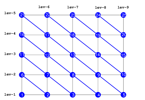
Fig. 1: Level scheduling for the 5-point stencil operator a 2-D regular grid

4.2 Self-scheduling algorithms

The level-scheduling algorithms discussed in the previous section have a main drawback of including a global synchronization point between two levels. It is not only that the synchronization itself represents an extra overhead but the synchronization can also stall jobs that are ready to go. In the example shown in Figure 1, suppose that when dealing with level 5, computations on nodes 5, 9 and 13 are finished much earlier than those on 17 and 21. In the level-scheduling schemes, the computations on nodes 10 and 14 will not be started until the entire level 5 finishes although nodes 10 and 14 are free of dependencies immediately after the jobs on nodes 5, 9 and 13 are done. This issue motivated the development of the self-scheduling algorithms that can dynamically schedule the computations on the nodes that are ready and can avoid global synchronizations.

In the self-scheduling algorithms, each node (or equivalently, each unknown) maintains a counter of the nodes that it depends on that have not finished. Once the counter reaches zero, it means that it is ready to solve its unknown. A sketch of the row-wise self-scheduling algorithm is given in Algorithm 3, where additional auxiliary data for the matrix are required that are the column pointers $ib$ and the row indices $jb$ as in the CSC format. Lines 2–4 make up a busy-waiting loop that iterates until there are no unfinished dependencies for node $i$. In line 11, the counters of the nodes that depend on $i$ are decreased by 1, and we remark that line 11 should be put inside a critical region since the decrements can be executed in parallel from different unknowns.

Algorithm 3 SLFR: Row-wise forward substitutions with self-scheduling

1:  for $i=1,2,\ldots,n$ do {rows in parallel}

2:     while $count(i)\neq 0$  do

3:        {do nothing}

4:     end while

5:     for $j=ia(i),\ldots,ia(i+1)-1$ do

6:        $x(i):=x(i)-a(j)\times x(ja(j))$

7:     end for

8:     $x(i):=x(i)/d(i)$

9:     for $j=ib(i),\ldots,ib(i+1)-1$ do

10:        CRITICAL SECTION ENTRY

11:        $count(jb(j)):=count(jb(j))-1$

12:        CRITICAL SECTION EXIT

13:     end for

14:  end for

The column-wise self-scheduling algorithm for forward substitutions is presented in Algorithm 4, which is based on the same counter-based scheme, and the input counters are identical to those used in the row-wise algorithm. Comparing with Algorithm 3, first this algorithm does not require additional inputs for the matrix other than the arrays in the CSC format. Second, Algorithm 4 uses the same column-wise updating scheme as the fundamental column-wise algorithm shown in Section 3.2, so that the updates to the solution vector $x$ need to be put into a critical region as well. Finally, if we take a closer look at the execution order of the computations in this algorithm, we find that this algorithm actually uses an even more “aggressive” scheduling scheme for concurrency than the row-wise self-scheduling algorithm, which is illustrated in the example shown in Figure 2.

Algorithm 4 SLFC: Column-wise forward substitutions with self-scheduling

1:  for $i=1,2,\ldots,n$ do {columns in parallel}

2:     while $count(i)\neq 0$  do

3:        {do nothing}

4:     end while

5:     $x(i):=x(i)/d(i)$

6:     for $j=ib(i),\ldots,ib(i+1)-1$ do

7:        CRITICAL SECTION ENTRY

8:        $x(jb(j))=x(jb(j))-b(j)\times x(i)$

9:        $count(jb(j)):=count(jb(j))-1$

10:        CRITICAL SECTION EXIT

11:     end for

12:  end for

In Figure 2, we show a situation where solving $x(i)$ depends on the solutions of $x(j_{1})$, $x(j_{2})$ and $x(j_{3})$. In Algorithm 3, the reduction operations (lines 5–7) for computing $x(i)$ are not started until the solutions for $j_{1}$, $j_{2}$ and $j_{3}$ are all available. A more aggressive strategy is to immediately start the computations when individual solutions become available and save the partial results in $x(i)$. Specifically, suppose that $x(j_{1})$ is available earlier than $x(j_{2})$ and $x(j_{3})$. Then, the partial result $L_{i,j_{1}}x(j_{1})$ can be computed and subtracted from $x(i)$ while waiting for the solutions of $x(j_{2})$ and $x(j_{3})$. This is essentially how the computations are scheduled in the column-wise algorithm. Clearly, there is a finer-level concurrency in Algorithm 4 than Algorithm 3 at the price of having a bigger critical region.

Fig. 2: An illustration of the operations for solving $x(i)$ in the row-wise forward substitution

4.3 CUDA implementations

We implemented the four aforementioned SpTrSv algorithms in CUDA for NVIDIA GPUs, namely they are the row-wise level-scheduling algorithm (LEVR), the column-wise level-scheduling algorithm (LEVC), the row-wise self-scheduling algorithm (SLFR), and the column-wise self-scheduling algorithm (SLFC). In this section, we discuss the implementations of these CUDA kernels in turn. Only the implementations of forward substitution will be presented. The implementations of backward substitution are straightforward.

We shall start with kernel LEVR that is a CUDA implementation of Algorithm 1. The input x is the solution vector that is assumed to have been initialized as the right-hand side before the entry of this function. Arrays ia, ja and a contain the strictly lower triangular matrix in the CSR format, while the diagonal is stored in vector d separately. Array jlev contains the indices of the unknowns that are grouped by levels, and l1 and l2 are the pointers of the starting positions of the current group and the next. The information in jlev, l1 and l2 are assumed to have been obtained from the setup phase.

⬇

1__global__ void LEVR(REAL *x, REAL *a, int *ja, int *ia, REAL *d,

2 int *jlev, int l1, int l2) {

3 int wid = (blockIdx.x*BLOCKDIM+threadIdx.x)/WARP;

4 int lane = threadIdx.x & (WARP-1);

5 volatile __shared__ REAL r[BLOCKDIM+16];

6 if (wid >= l2-l1) return;

7 int i = jlev[l1+wid];

8 int p1 = ia[i], q1 = ia[i+1];

9 REAL sum = 0.0;

10 for (int k=p1+lane; k<q1; k+=WARP)

11 sum += a[k] * x[ja[k]];

12 r[threadIdx.x] = sum; // parallel reduction

13 r[threadIdx.x] = sum = sum + r[threadIdx.x+16];

14 r[threadIdx.x] = sum = sum + r[threadIdx.x+8];

15 r[threadIdx.x] = sum = sum + r[threadIdx.x+4];

16 r[threadIdx.x] = sum = sum + r[threadIdx.x+2];

17 r[threadIdx.x] = sum = sum + r[threadIdx.x+1];

18 if (lane == 0)

19 x[i] = (x[i] - r[threadIdx.x]) / d[i];

20}

In the function LEVR, one warp of threads, a CUDA concept that means $32$ consecutive threads (i.e., $\mathtt{WARP}\equiv 32$), are dispatched for one unknown of the current level and thus access one row of the matrix associated with their global warp index (line 7), namely wid. The CUDA built-in variables blockIdx and threadIdx contain the block index and the thread index within the block, and the constant BLOCKDIM is the dimension of the block. The dot-product operations between the sparse row i and vector x are performed by the parallel reduction within the warp (lines 10–17) in the array r located in the shared memory. Finally, the first thread of the warp, which is the one with lane == 0, saves the result back to x(i).

Next, we will see the CUDA implementation of Algorithm 2 that is shown in the kernel function LEVC, where the inputs ib, jb and b are the sparse lower triangular matrix in the CSC format. The variable wlane is the local warp index in the thread block. The critical section in Algorithm 2 is implemented by using the CUDA atomicAdd operation. An optimization used here on memory transactions is to let only the first thread of a warp compute x(i) and save the result into s_xi in the shared memory, and then let all the other threads of the same warp read this value from s_xi. A small performance gain has been observed by this optimization compared with letting all the threads in the warp compute xi.

⬇

1__global__ void LEVC(REAL *x, REAL *b, int *jb, int *ib, REAL *d,

2 int *jlev, int l1, int l2) {

3 int wid = (blockIdx.x*BLOCKDIM+threadIdx.x)/WARP;

4 int lane = threadIdx.x & (WARP-1);

5 int wlane = threadIdx.x / WARP;

6 volatile __shared__ REAL s_xi[BLOCKDIM/WARP];

7 if (wid >= l2-l1) return;

8 int i = jlev[l1+wid];

9 if (lane == 0) s_xi[wlane] = x[i]/d[i];

10 REAL xi = s_xi[wlane];

11 int p1 = ib[i], q1 = ib[i+1];

12 for (int j=p1+lane; j<q1; j+=WARP)

13 atomicAdd(&x[jb[j]], -xi*b[j]);

14 if (lane == 0) x[i] = xi;

15}

The above two kernel functions solve all the unknowns in one level at a time, so that the entire forward substitutions can be done by repeatedly running the functions in an outer-loop as shown in the following, since the easiest way to achieve global synchronization in CUDA is to launch a new kernel after the current one finishes.

⬇

1for (int i=0; i<nlev; i++) { /* ilev: level pointers */

2 LEVR<<<...,...>>>(x, a, ja, ia, d, jlev, ilev(i), ilev(i+1);

3}

In the rest of this section, we discuss the CUDA kernels that implement the self-scheduling algorithms. The kernel function SLFR implements the row-wise self-scheduling approach in Algorithm 3. Since this algorithm requires column access to the nonzero pattern of the matrix, column pointers ib and row indices jb are also provided as inputs in addition to the CSR format matrix ia, ja and a. On the entry of this function, array dp contains the count of dependencies for each unknown and it contains all zeros on exit. The input array jlev has the same meaning as the one in the kernel functions LEVR and LEVC.

⬇

1__global__ void SLFR(int n, REAL *x, REAL *a, int *ja, int *ia,

2 REAL *d, int *jb, int *ib, int *dp, int *jlev) {

3 int wid = (blockIdx.x*BLOCKDIM+threadIdx.x)/WARP;

4 int lane = threadIdx.x & (WARP-1);

5 volatile __shared__ REAL r[BLOCKDIM+16];

6 REAL ti, xi, sum = 0.0;

7 if (wid >= n) return;

8 int i = jlev[wid];

9 int p1 = ia[i], q1 = ia[i+1];

10 int p2 = ib[i], q2 = ib[i+1];

11 if (lane == 0) {

12 ti = 1.0 / d[i]; xi = x[i];

13 while (((volatile int *)dp)[i] != 0);

14 }

15 for (int k=p1+lane; k<q1; k+=WARP)

16 sum += a[k]*x[ja[k]];

17 r[threadIdx.x] = sum; // parallel reduction

18 r[threadIdx.x] = sum = sum + r[threadIdx.x+16];

19 r[threadIdx.x] = sum = sum + r[threadIdx.x+8];

20 r[threadIdx.x] = sum = sum + r[threadIdx.x+4];

21 r[threadIdx.x] = sum = sum + r[threadIdx.x+2];

22 r[threadIdx.x] = sum = sum + r[threadIdx.x+1];

23 if (lane == 0) {

24 x[i] = (xi - r[threadIdx.x]) * ti;

25 __threadfence();

26 }

27 for (int j=p2+lane; j<q2; j+=WARP)

28 atomicSub(&dp[jb[j]], 1);

29}

In the function SLFR, the busy-waiting loop is at line 13, where the counter of unknown $x(i)$ is constantly being compared with zero. The keyword volatile is used to tell the compiler that this variable can be changed at any time by other threads [44]. Once the warp breaks out of the busy loop, it proceeds with the parallel reduction as in LEVR. In line 28, the counters of the unknowns that depend on i are decreased by one using the atomicSub operation. Note that a “thread fence” is put up after updating x[i] by the first thread of a warp and before decreasing the counters. This is to guarantee that at the time when the threads working on the unknowns that depend on i see the corresponding counters equal to zeros, the updates to x[i] have already been observed by all the threads in the device [44].

Finally, we discuss the implementation of the column-wise self-scheduling approach in Algorithm 4, which is given in the kernel function SLFC. The CSC format matrix in ib, jb and b is given as an input and the other inputs and outputs are the same as those of SLFR. The function SLFC uses the same counter-based busy-waiting scheme as in SLFR and uses the same implementation of the column-wise updates to $x$ as in LEVC. Again, as in LEVC, the shared memory array s_xi is used to save the result of xi computed by the first thread of a warp.

⬇

1__global__ void SLFC(int n, REAL *x, REAL *b, int *jb, int *ib,

2 REAL *d, int *dp, int *jlev) {

3 int wid = (blockIdx.x*BLOCKDIM+threadIdx.x)/WARP;

4 int wlane = threadIdx.x / WARP;

5 int lane = threadIdx.x & (WARP - 1);

6 volatile __shared__ REAL s_xi[BLOCKDIM/WARP];

7 if (wid >= n) return;

8 int i = jlev[wid];

9 int p1 = ib[i], q1 = ib[i+1];

10 REAL ti, xi;

11 if (lane == 0) {

12 ti = 1.0 / d[i];

13 while (((volatile int *)dp)[i]);

14 xi = x[i] * ti; s_xi[wlane] = xi;

15 }

16 xi = s_dx[wlane];

17 for (int j=p1+lane; j<q1; j+=WARP) {

18 atomicAdd(&x[jb[j]], -xi*b[j]);

19 __threadfence();

20 atomicSub(&dp[jb[j]], 1);

21 }

22 if (lane == 0) x[i] = xi;

23}

Before closing this section, we remark that a similar method to Algorithm 4 was adopted in the “global-synchronization-free” algorithm proposed in [34]. We list the major differences between the two algorithms and their implementations as follows:

1. In the forward substitution in [34], a warp is dispatched to the unknown with the global index of the warp, i.e., wid in functions SLFR and SLFC. However, in our algorithms, the mapping between warps and the unknowns respects the order in jlev, where the unknowns are listed in a non-descending order of their levels (see line 8 of SLFR and SLFC for the assignments of the warps to the unknowns). From our experimental results, we found that this warp-unknown mapping can often significantly reduce the waiting time and thus can yield much higher overall performance. On the negative side, our algorithms require the level information as input which is not needed by the algorithms in [34]. Consequently, the setup phase of our algorithms will be more costly for computing the levels.

2. In our algorithms, since warps with consecutive indices in a CUDA block in general do not work on consecutive unknowns, the optimization used in [34] that utilizes the shared memory to perform partial updates to the dependent counters in dp and the solution x cannot be applied directly. However, this optimization can still be used if we preorder the matrix columns according to the levels of the corresponding unknowns. Nevertheless, in this work we do not assume that the original matrix has been reordered.

3. In our implementations of the self-scheduling algorithms, only the first thread of a warp is spinning on the lock (line 13 in SLFR and SLFC), whereas the other threads of the warp will wait for the first thread to break its busy-waiting loop before proceeding to the later instructions. This coordination is actually guaranteed by the warp-level synchronization, that is, a warp can only execute one common instruction at a time and warp divergence is serialized. On the other hand, in [34], the whole warp is spinning.

It turns out that the above differences have significant performance effects. As we show in the experimental results in Section 5, our implementations of the self-scheduling algorithms exhibit superior performance compared with the implementation of the synchronization-free algorithm in [34].

4.4 Setup phases

All the parallel SpTrSv algorithms discussed in this paper require a setup phase, where the parallelism in the solve phase is discovered from the nonzero pattern of the sparse triangular matrix. The justification of paying the extra cost at the setup phase but having a more efficient solve phase has been discussed at the end of Section 1. In this section, we examine the operations required in the setup phases of the algorithms discussed in the previous section. Table 1 tabulates the major steps in the setup phases, where the first column lists the setup phases of the different SpTrSv algorithms. “*_CPU” and “*_GPU” indicates whether the setup phase is running on the CPU or on the GPU.

Table 1: The operations required in the setup phases of different SpTrSv algorithms

	MAT_D2H	TRANS_GPU	DEP_GPU	LEV_CPU	LEV_GPU	LEV_H2D
LEVR_CPU	✓			✓		✓
LEVR_GPU		✓	✓		✓
LEVC_CPU	✓			✓		✓
LEVC_GPU			✓		✓
SLFR_CPU	✓	✓	✓	✓		✓
SLFR_GPU		✓	✓		✓
SLFC_CPU	✓		✓	✓		✓
SLFC_GPU			✓		✓
GSF_GPU			✓

In the setup phases of the level-scheduling algorithms, namely LEVR and LEVC, the major computation is to decide the level of each unknown. To do this computation on the CPU, indicted by “LEV_CPU” in the table, the implementations are straightforward. They are simply the two for-loops presented at the beginning of Section 4.1, for matrices in row-wise storage formats and column-wise storage formats respectively. These two for-loops require operations of the order of the number of the nonzeros of the matrix and are generally hard to parallelize. Moreover, when the level information is computed on the host, memory transfers between the host and the device are also needed, since the matrices are assumed to be stored on the device and the computed array $jlev$ is required on the device. The memory copies are denoted by “MAT_D2H” and “LEV_H2D” in the table.

In the setup phases of the self-scheduling algorithms, SLFR and SLFC, computing the level information is also involved. Additionally, the numbers of the dependents of all the unknowns are required as well, which can be easily obtained by counting the number of nonzeros per row. This operation is denoted by “DEP_GPU”. Since both of the self-scheduling algorithms require column-wise access to the matrices, the setup phase of algorithm SLFR also includes a transposition step, in which we transpose the CSR matrices on the GPU (nonzero pattern only without numerical values) to obtain the matrices in the CSC format. This transposition step is denoted by “TRANS_GPU” in the table. On the other hand, the setup phase of the synchronization-free algorithm in [34] is the simplest, which only requires the dependent counters and the cost of which is almost free.

Among all these aforementioned operations in the setup phases, calculating the levels turns out to be the most expensive computation compared with the costs of the other operations, which are basically negligible. Attempts have been made to accelerate this computation by performing a parallel topological sorting algorithm, namely Kahn’s algorithm [45], on GPUs, which is labeled as “LEV_GPU” in Table 1. In the next section, we will discuss the CUDA implementation of this algorithm.

4.4.1 Implementing Kahn’s algorithm in CUDA

The idea of Kahn’s algorithm is to perform topological sorting on the DAG by repeatedly finding vertices of in-degree zero, which are called roots, saving the roots of the current level into a queue, and removing the roots and their outgoing edges from the graph. This algorithm was first described by Kahn in 1962 and also can be found in [46]. To the best of our knowledge, the first CUDA implementation of this algorithm was due to Naumov [31] with a modified form of parallel breadth first search (BFS).

To start Kahn’s algorithm, the output queue should be first initialized with the roots of level 0. The kernel function FIND_LEVEL0 shown below performs this initialization, where dp contains the dependent counters, jlev implements the queue, and last points to the past-the-end position of the elements in the queue, which should be set to zero on entry. As shown in this function, the level-0 roots are found in parallel and saved into jlev, and last is raised by the atomicAdd operation.

⬇

1__global__ void FIND_LEVEL0(int n, int *dp, int *jlev, int *last) {

2 int gid = blockIdx.x * BLOCKDIM + threadIdx.x;

3 if (gid >= n) return;

4 if (dp[gid] == 0)

5 jlev[atomicAdd(last, 1)] = gid;

6}

After the initialization step for level 0, roots of the succeeding levels can be computed by the kernel function FIND_LEVEL. The input first is the starting position of the current level in jlev. This function requires the inputs of column pointers in ib and row indices in jb as well for retrieving the information of the outgoing edges of vertices. Therefore, the transposition is also required in the setup phase of algorithm LEVR, if it is running on GPUs. When the outgoing edges are removed, the counters in dp will be lowered accordingly. Whenever a counter reaches zero, the corresponding vertex is added to the queue and the ending position of the current level, stored in last, is increased by one.

⬇

1__global__ void FIND_LEVEL(int *ib, int *jb, int *dp, int *jlev,

2 int first, int *last) {

3 int wid = (blockIdx.x * BLOCKDIM + threadIdx.x) / WARP;

4 int lane = threadIdx.x & (WARP - 1);

5 int i = jlev[first+wid];

6 int p1 = ib[i], q1 = ib[i+1];

7 for (int j=p1+lane; j<q1; j+=WARP)

8 if (atomicSub(&dp[jb[j]], 1) == 1)

9 jlev[atomicAdd(last, 1)] = jb[j];

10}

Clearly, the entire topological sort can be performed by repeatedly calling function FIND_LEVEL until all the vertices have been removed from the graph, as shown in the code segment below. The graph is traversed one level at a time, and between two levels there is a synchronization point by restarting the kernel function and a memory transfer from the device to the host for the number of the vertices that have been removed so far. Consequently, like the level-scheduling algorithms in the solve phases, the efficiency will gradually deteriorate with the increase of the number of levels. A more efficient implementation of Kahn’s algorithm in CUDA without global synchronization is currently being investigated by the author.

⬇

1 FIND_LEVEL0<<<..., ...>>>(n, dp, jlev, last);

2 cudaMemcpy(&h_last, last, sizeof(int), cudaMemcpyDeviceToHost);

3 for (first=0, nlev=0, ilev[0]=0; h_last < n; ) {

4 FIND_LEVEL<<<..., ...>>>(ib, jb, dp, jlev, first, last);

5 cudaMemcpy(&h_last, last, sizeof(int), cudaMemcpyDeviceToHost);

6 first = h_last; ilev[nlev++] = first;

7 }

8 ilev[nlev] = n;

5 Numerical experiments

The experiments were conducted on one node of Ray, a Linux cluster at Lawrence Livermore National Laboratory, equipped with a dual socket Power 8+ CPU (10 cores/socket) and 4 NVIDIA Tesla P100 (Pascal) GPUs. The CUDA program was compiled by the NVIDIA CUDA compiler nvcc from CUDA toolkit 8.0 with option -gencode arch=compute_60,"code=sm_60" for compute capability 6.0, and the CPU code was compiled by IBM C++ compiler xlc++ with the -O2 optimization level. For the CUDA kernel configurations, thread blocks are one-dimensional and of size 512. We compared our four SpTrSv solvers that are LEVR and LEVC using the level-scheduling algorithm and SLFR and SLFC using the self-scheduling algorithm, with the two solvers cusparse?csrsv and cusparse?csrsv2 available from cuSPARSE v8.0. The cusparse?csrsv solver adopted a similar row-wise level-scheduling approach as in LEVR [31], whereas the algorithm used in cusparse?csrsv2 has not been published. We also considered the global-synchronization-free algorithm introduced in [34], denoted by GSF, the implementation of which is available from [47]. In the following of this section, we will first show the performance of these solvers on structured matrices obtained from finite difference discretizations of 2-D and 3-D Laplace operators, and then we will report their performance on general matrices.

For each test matrix $A\in\mathbb{R}^{n\times n}$, letting

$$A=L+D+U,$$ (2)

where $L$ and $U$ denote the strict lower and upper triangular parts of $A$ respectively, and $D$ denotes the diagonal matrix that has the same diagonal as $A$, for which we assume that $D_{ii}\neq 0$ for $i=1,\ldots,n$, we solve the lower triangular system followed by the upper triangular system of the form

$$y=(U+D)^{-1}(L+D)^{-1}x.$$ (3)

The performance of the solves in (3) was measured in GFLOPS given by

$$\mbox{GFLOPS}=\frac{2\times nnz}{t\times 10^{9}},$$ (4)

where we denote by $nnz$ the number of nonzeros of $A$ and by $t$ the solve time measured in seconds, which was taken as an average of 100 runs. Note that in (4) the factor $2$ is due to the fact that each off-diagonal nonzero entry requires one addition and one multiplication and there are two divisions for each diagonal element.

For the row-wise algorithms, we assume that the matrix $A$ is stored in the CSR format on the GPU, whereas for the CSC format we assume that $A$ is available in the CSC format on the GPU.

5.1 2-D and 3-D Laplacians

We shall start our performance study with a set of discretized Laplacians obtained from the finite-difference scheme on regular grids of the dimension $n_{x}\times n_{y}\times n_{z}$. The size of the matrix, denoted by $n$, is given by $n=n_{x}n_{y}n_{z}$. In Table 2, we list the dimensions of the testing grids, where $\rho_{yx}$ and $\rho_{zx}$ are the aspect ratios of the grids defined as

$$\rho_{yx}=\frac{n_{y}}{n_{x}}\quad\mbox{and}\quad\rho_{zx}=\frac{n_{z}}{n_{x}}\ .$$ (5)

In general, the numbers of the levels in the sparse triangular systems of the same size will increase with these ratios and thus the degrees of parallelism will decrease accordingly. Therefore, lower performance will be expected for the grids with higher aspect ratios. In this set of experiments, we will examine the performance behaviors of the 7 considered solvers across the testing grids. For the 2-D grids, we tested Laplacian matrices with standard $5$- and $9$-point stencils, while for the 3-D grids we tested the standard $7$- and $27$-point Laplacian matrices. The number of stencil points is precisely the number of nonzeros of a matrix row that does not correspond to a grid point on the boundary. Moreover, this number is also the same as the number of the diagonals of the matrix under the assumption that the lexicographical ordering is used for the grid points.

Table 2: 2-D/3-D regular grids for generating Laplacian matrices

$n_{x}\times n_{y}$	$\rho_{yx}$	$n_{x}\times n_{y}\times n_{z}$	$\rho_{zx}$
$1024\times 1024$	1	$128\times 128\times 128$	1
$512\times 2048$	4	$64\times 128\times 256$	4
$256\times 4096$	16	$64\times 64\times 512$	8
$128\times 8192$	64	$32\times 64\times 1024$	32
$64\times 16384$	256	$32\times 32\times 2048$	64

In Figures 3 and 4, we present the performance of the solve phases of the triangular solves in (3) that is measured in GFLOPS in both single and double precisions for 2-D and 3-D Laplacians on the regular grids listed in Table 2. The solvers cusparse?_csrsv and cusparse?_csrsv2 from cuSPARSE are denoted by CUS1 and CUS2 respectively in the figures. The x-axes of the figures represent the aspect ratios $\rho_{yx}$ and $\rho_{zx}$ that are defined in (5). For the results of the 2-D Laplacians in Figure 3, for most of the cases, LEVR and LEVC outperformed the cuSPARSE counterpart cusparse?_csrsv, and the self-scheduling solvers SLFR and SLFC showed superior performance to the level-scheduling solvers. For all the grids, the column-wise algorithm SLFC exhibited better performance than the row-wise algorithm SLFR and the performance of SLFC was very close to that of cusparse?_csrsv2. As expected, the performance of all the first 6 solvers steadily degraded when the ratios $\rho_{yx}$ and $\rho_{zx}$ were increasing. On the other hand, GSF was the exception, which performed exceedingly poorly for the first two grids but eventually became competitive again for the last two grids. For all the grids and all the solvers, the performance difference between the kernels in single precision and double precision was very small.

Fig. 3: Performance of the solve phases of the SpTrSv algorithms for 2-D Laplacians on regular grids in single and double precisions measured in GFLOPS

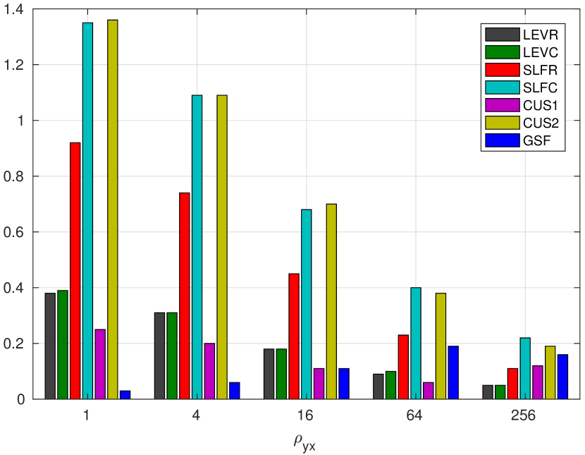
(a) 5-point stencil, single precision

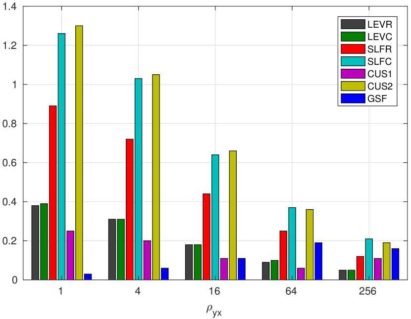
(b) 5-point stencil, double precision

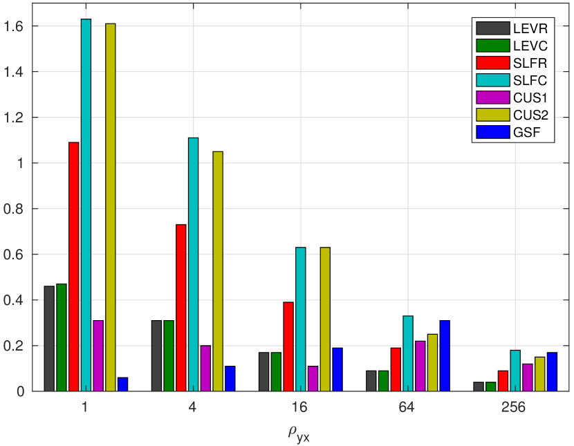
(c) 9-point stencil, single precision

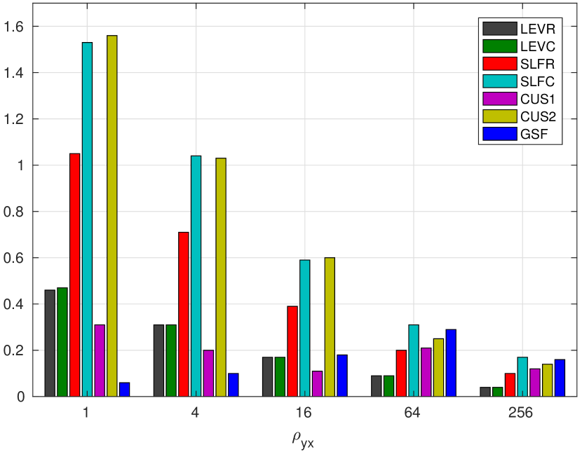
(d) 9-point stencil, double precision

The performance for the 3-D Laplacians are shown in Figure 4. Compared with the 2-D problems, the GFLOPS numbers are much higher. This is because first there are much fewer levels in the triangular matrices for these 3-D problems, and second there are more operations in each task due to the more complex stencils. When comparing the different solvers, the level-scheduling approaches LEVR and LEVC were faster than the row-wise self-scheduling solver SLFR for most of the 7-point operators, while the column-wise solver SLFC remained the fastest for all the test cases except for the 7-point operator on the last 3-D grid, where cusparse?_csrsv2 slightly outperformed SLFC (3.11 vs. 3.05 GFLOPS in single precision and 2.98 vs. 2.84 GFLOPS in double precision). For the other cases, the speedup of SLFC over cusparse?_csrsv2 was by a factor of from $1.18$ to $1.47$ for the 7-point matrices and from $1.09$ to $1.82$ for the 27-point matrices. For almost all the 3-D Laplacians, the performance of the GSF solver was lower than those of the other solvers, and in particular the performance gap between the GSF solver and the self-scheduling solvers was quite significant. Finally, we remark that the performance discrepancy between single and double precisions was more noticeable for the 3-D problems than that for the 2-D problems.

Fig. 4: Performance of the solve phases of the SpTrSv algorithms for 3-D Laplacians on regular grids in single and double precisions measured in GFLOPS

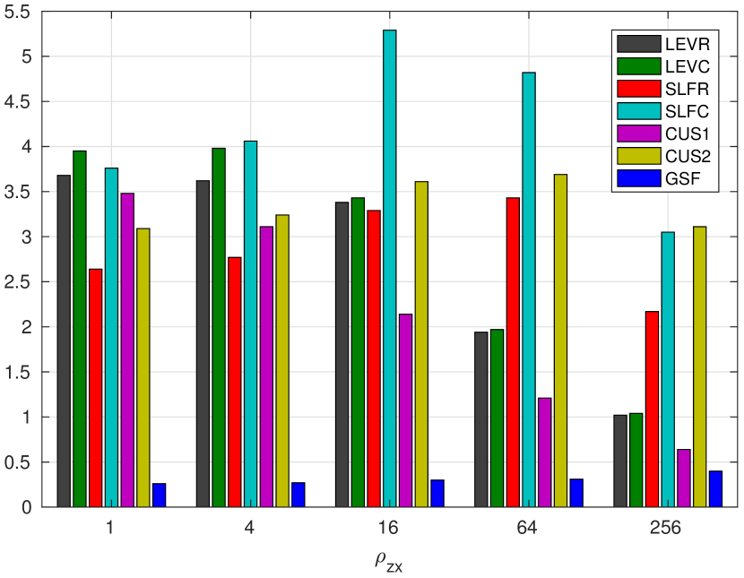
(a) 7-point stencil, single precision

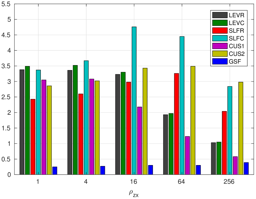
(b) 7-point stencil, double precision

(c) 27-point stencil, single precision

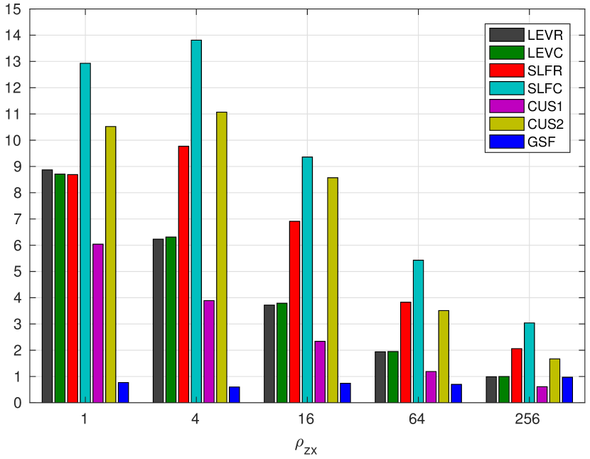
(d) 27-point stencil, double precision

5.2 General matrices

In this section, we report the performance of the SpTrSv solvers in CUDA on $10$ general matrices selected from the University of Florida sparse matrix collection [48] and $2$ matrices for linear elasticity problems discretized with linear elements generated by the finite element package MFEM [49]. The size (N), the number of the nonzeros (NNZ), the average number of non-zeros per row (RNZ), and a short description of each matrix are tabulated in Table 3. The sizes of these matrices range from half a million to 4 million, and the densities of the matrices vary from a few nonzeros per row to several scores.

Table 3: Names, orders (N), numbers of nonzeros (NNZ), average numbers of nonzeros per row (RNZ), and short descriptions of the test matrices.

Matrix	N	NNZ	RNZ	DESCRIPTION
af_shell8	504,855	17,588,875	34.8	Sheet metal forming simulation
ecology2	999,999	4,995,991	5.0	Landscape ecology problem
webbase1M	1,000,005	3,105,536	3.1	Web connectivity matrix
elasticity2D	1,002,528	14,012,744	14.0	2D FEM elasticity
elasticity3D	1,029,000	80,990,208	78.7	3D FEM elasticity
thermal2	1,228,045	8,580,313	7.0	Steady state thermal problem
atmosmodd	1,270,432	8,814,880	6.9	Atmospheric modeling problem
StocF-1465	1,465,137	21,005,389	14.3	Flow in porous medium problem
af_shell10	1,508,065	52,672,325	34.9	Sheet metal forming simulation
Transport	1,602,111	23,500,731	14.7	3D FEM flow and transport
Bump_2911	2,911,419	127,729,899	43.8	3D reservoir simulation
Queen_4147	4,147,110	329,499,284	79.4	3D structural problem

In Figure 5, we report the performance of the 7 tested solvers in double precision only. The numbers of the levels in the lower and upper triangular parts of the matrices are presented at the bottom of this figure. As shown, our LEVR and LEVC solvers consistently outperformed the cuSPARSE counterpart cusparse?_csrsv, and our SLFC solver achieved speedup over cusparse?_csrsv2 by a factor of up to $2.64$. The highest GFLOPS numbers ($>10$ GFLOPS) were achieved with matrices elasticity3D and Queen_4147, both of which have denser rows (about 79 nonzeros per row) than the other matrices. Note that although there are a large number of levels in Queen_4147, the self-scheduling algorithms still reached high performance in the solves. Lastly, for most of the matrices, the performance of the GSF solver was not very competitive compared with the other solvers.

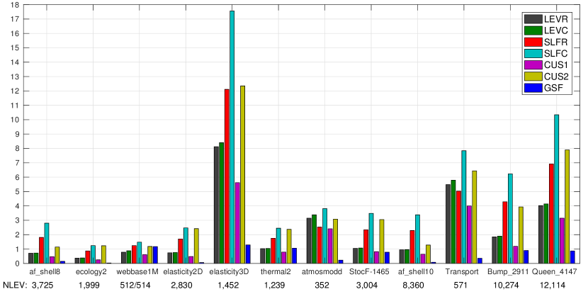
Fig. 5: The numbers of the levels (NLEV) in the lower and upper triangular parts of the tested matrices and the performance of the solve phases of the SpTrSv algorithms, measured in GFLOPS and in double precision.

5.3 Cost of the setup phases

Our final experimental results to report are the timings of the setup phases of all the sparse triangular system solvers considered in this paper. In Table 4, we present the timings required by these setup phases running the CPU, which were measured in milliseconds. In this table, the numbers in the parentheses are the ratios between the setup time and the time for one solve of (3) in double precision. As shown, the setup time for the 2-D problems was generally small, not much more expensive than the solve time. Moreover, the timings for running the setup phases on the CPU was almost constant for the various shapes of grids. Since the performance of the solve phases gradually degrades for grids with higher aspect ratios, the cost of the setup phase became more and more insignificant relative to the cost of the solve phase. The time differences in the setup phases between LEVR and LEVC and between SLFR and SLFC were due to the two versions of the sequential algorithms running the CPU for computing the levels of the unknowns. Based on the experimental results, the column-wise version was often faster than the row-wise version except for the 2-D 5-point operators. On the other hand, the setup costs for the 3-D problems were much higher due to the more complex stencils. Compared with the cost of the setup phase of cusparse?_csrsv, the setup phases of our solvers were always cheaper for all problems when running the CPU. The cost of the setup phase of cusparse?_csrsv2 was in general the most inexpensive, especially for the 3-D problems, among all the solvers except for GSF, whereas the setup cost of GSF was basically negligible but the performance of its solve phase has been shown to be usually much lower than those of the others.

Table 4: Timings of the setup phases of the SpTrSv algorithms running on the CPU for the 2-D and 3-D Laplacians on regular grids, measured in milliseconds. The numbers in the parentheses are the ratios between the setup time and the time for one solve of (3) in double precision.

(a) 2-D Laplacians with 5-point stencil

LEVR	LEVC	SLFR	SLFC	CUS1	CUS2	GSF
030 (1.1)	041 (1.5)	034 (2.9)	041 (5.0)	086 (2.1)	214 (27.)	.34 (.00)
30 (.87)	41 (1.2)	34 (2.4)	42 (4.1)	94 (1.8)	75 (7.5)	.34 (.00)
30 (.51)	41 (.72)	34 (1.5)	41 (2.5)	128 (1.4)	36 (2.3)	.35 (.00)
30 (.27)	41 (.38)	34 (.81)	41 (1.5)	203 (1.2)	25 (.87)	.34 (.00)
30 (.14)	41 (.19)	34 (.40)	41 (.85)	357 (3.8)	35 (.64)	.35 (.00)

(b) 2-D Laplacians with 9-point stencil

LEVR	LEVC	SLFR	SLFC	CUS1	CUS2	GSF
045 (1.1)	036 (.90)	052 (2.9)	036 (2.9)	120 (2.0)	208 (17.)	.41 (.00)
45 (.71)	36 (.59)	52 (2.0)	37 (2.0)	151 (1.6)	74 (4.0)	.40 (.00)
44 (.39)	36 (.32)	52 (1.1)	36 (1.1)	223 (1.3)	37 (1.2)	.40 (.00)
44 (.20)	36 (.17)	52 (.54)	36 (.60)	377 (4.2)	36 (.47)	.40 (.01)
44 (.10)	36 (.08)	52 (.27)	36 (.33)	688 (4.4)	79 (.61)	.39 (.00)

(c) 3-D Laplacians with 7-point stencil

LEVR	LEVC	SLFR	SLFC	CUS1	CUS2	GSF
077 (8.9)	065 (7.8)	089 (7.4)	065 (7.5)	116 (12.)	044 (4.3)	.76 (.01)
75 (8.7)	64 (7.7)	86 (7.8)	63 (7.9)	121 (13.)	55 (5.8)	.77 (.01)
75 (8.4)	64 (7.2)	86 (8.9)	63 (10.)	125 (9.2)	44 (5.2)	.76 (.01)
75 (5.0)	63 (4.3)	86 (9.7)	63 (9.7)	134 (5.6)	46 (5.6)	.75 (.01)
75 (2.7)	64 (2.3)	86 (6.1)	64 (6.3)	134 (3.0)	34 (3.5)	.75 (.01)

(d) 3-D Laplacians with 27-point stencil

LEVR	LEVC	SLFR	SLFC	CUS1	CUS2	GSF
253 (20.)	189 (15.)	285 (22.)	189 (22.)	289 (16.)	64 (6.0)	1.9 (.01)
252 (14.)	186 (11.)	287 (25.)	188 (23.)	302 (11.)	96 (9.4)	1.9 (.01)
249 (8.3)	187 (6.4)	286 (17.)	191 (16.)	308 (6.4)	82 (6.3)	1.9 (.01)
250 (4.3)	189 (3.4)	281 (9.1)	190 (9.4)	351 (3.8)	108 (3.4)	1.9 (.01)
247 (2.2)	186 (1.7)	282 (5.2)	189 (5.3)	406 (2.3)	74 (1.1)	1.9 (.01)

In Table 5, we report the timings for the setup phases on the GPU for the 2-D and 3-D Laplacians. Comparing with the results in Table 4, we can see that the setup phases on the GPU required more time than the CPU versions for the 2-D cases, whereas for the 3-D problems, the costs of the setup phases were reduced dramatically by the GPU. A remarkable difference between the GPU setup phases and the CPU ones is that the running time increases with the number of levels for the same reason as in the solve phases based on level-scheduling algorithms: the cost of (re)launching GPU kernels becomes higher when the number of levels is larger. The same performance behavior can be also found from the cost of the setup phase of the solver cusparse?_csrsv shown in Table 4. On the other hand, there is no clear evidence that the observed setup cost of cusparse?_csrsv2 is correlated with the number of levels.

Table 5: Timings of the setup phases of the SpTrSv algorithms running on the GPU for the 2-D and 3-D Laplacians on regular grids, measured in milliseconds. The numbers in the parentheses are the ratios between the setup time and the time for one solve of (3) in double precision.

(a) 2-D Laplacians with 5-point stencil

LEVR	LEVC	SLFR	SLFC
34 (1.2)	27 (1.0)	31 (2.7)	26 (3.2)
35 (1.0)	28 (.82)	32 (2.3)	27 (2.7)
39 (.66)	32 (.56)	36 (1.6)	31 (1.9)
56 (.50)	49 (.45)	53 (1.4)	48 (1.8)
95 (.43)	88 (.41)	92 (1.1)	87 (1.8)

(b) 2-D Laplacians with 9-point stencil

LEVR	LEVC	SLFR	SLFC
40 (.97)	29 (.72)	37 (2.1)	29 (2.4)
43 (.70)	33 (.54)	40 (1.6)	32 (1.8)
58 (.51)	47 (.42)	54 (1.1)	46 (1.5)
93 (.42)	82 (.38)	90 (.88)	82 (1.4)
167 (.38)	156 (.36)	164 (.86)	156 (1.4)

(c) 3-D Laplacians with 7-point stencil

LEVR	LEVC	SLFR	SLFC
39 (4.3)	22 (2.5)	34 (2.4)	21 (2.1)
41 (4.7)	23 (2.8)	36 (2.7)	23 (2.6)
50 (5.6)	33 (3.7)	47 (4.5)	33 (5.1)
62 (4.1)	46 (3.1)	57 (5.8)	45 (6.3)
73 (2.5)	59 (2.1)	70 (5.0)	58 (5.7)

(d) 3-D Laplacians with 27-point stencil

LEVR	LEVC	SLFR	SLFC
93 (7.3)	44 (3.4)	88 (6.6)	43 (4.9)
109 (6.1)	61 (3.5)	106 (8.9)	61 (7.0)
140 (4.7)	92 (3.1)	134 (8.3)	92 (7.6)
166 (2.9)	115 (2.1)	162 (5.8)	115 (5.6)
180 (1.6)	128 (1.2)	170 (3.3)	128 (3.6)

Finally, in Table 6, we present the cost of the setup phases for the general matrices listed in Table 3. In columns 2–5, the numbers outside the parentheses are the time required by the setup phases running on the CPU while the numbers in the parentheses are the setup time on the GPU. For 11 out of the 12 matrices, running the setup phases on the GPU provided speedups, and for 6 matrices the setup phase of the solver SLFC was cheaper than that of cusparse?_csrsv2.

Before closing the experimental results section, we use the general matrices to demonstrate the justification for paying extra cost in setup phases discussed in Section 1, by showing the smallest numbers of the solves, denoted by $n_{s}$, needed to make the SLFC solver have a shorter total time, i.e., find the smallest $n_{s}$ such that

$$T^{total}_{\mathtt{SLFC}}=T^{setup}_{\mathtt{SLFC}}+n_{s}\times T^{solve}_{\mathtt{SLFC}}<T^{setup}_{\mathtt{*}}+n_{s}\times T^{solve}_{\mathtt{*}}=T^{total}_{*},$$

where $T^{setup}_{*}$ and $T^{solve}_{*}$ denote the setup time and the solve time for a solver respectively. We will compute the $n_{s}$’s of SLFC and cusparse?_csrsv2 which are the two solvers that yielded the best performance in the solve phases in general for all the test matrices. We will also compute the $n_{s}$’s of SLFC and GSF as the GSF solver has an extremely inexpensive setup phase. These numbers are given in Table 7. As shown in the second column of the table, in order to beat cusparse?_csrsv2 in total time, the number of solves required does not need to be very large. It is often reasonable to assume to have such numbers of solves in the applications of iterative solvers. The zeros indicate the cases for which SLFC has a more efficient setup phase and the solve phases of SLFC are also faster than cusparse?_csrsv2. The numbers for GSF shown in the third column are very small since the solve phase performance of this solver is generally much worse, in spite of the very cheap setup phase needed by this solver.

Table 6: Timings of the setup phases of the SpTrSv algorithms running on the CPU and the GPU for the general matrices, measured in milliseconds.

Matrix	LEVR	LEVC	SLFR	SLFC	CUS1	CUS2	GSF
af_shell8	76 (88)	57 (71)	89 (85)	57 (70)	156	72	.43
ecology2	28 (32)	39 (26)	33 (30)	39 (25)	82	216	.34
webbase1M	33 (15)	32 (11)	37 (13)	33 (11)	59	8.0	1.0
elasticity2D	62 (62)	48 (47)	72 (59)	49 (47)	132	265	.46
elasticity3D	466 (127)	422 (61)	525 (120)	425 (61)	358	52	2.2
thermal2	55 (37)	57 (27)	62 (34)	57 (26)	94	11	.43
atmosmodd	46 (27)	38 (17)	54 (25)	38 (16)	80	29	.46
StocF-1465	103 (92)	101 (71)	118 (89)	102 (71)	184	24	.81
af_shell10	230 (200)	173 (154)	268 (195)	175 (154)	396	372	1.2
Transport	107 (50)	69 (27)	125 (46)	70 (27)	149	37	.90
Bump_2911	664 (354)	624 (250)	757 (344)	631 (251)	751	136	3.7
Queen_4147	1872 (726)	1676 (472)	2106 (710)	1690 (469)	1625	253	9.3

Table 7: The smallest numbers of solves required by SLFC to have a faster total time (setup time plus solve time) than cusparse?_csrsv2 and GSF for the general matrices.

Matrix	CUS2	GSF
af_shell8	0	1
ecology2	0	1
webbase1M	3	9
elasticity2D	0	1
elasticity3D	3	1
thermal2	61	3
atmosmodd	0	1
StocF-1465	28	2
af_shell10	0	1
Transport	0	1
Bump_2911	5	2
Queen_4147	11	1

6 Conclusions

This paper considers efficient parallel algorithms for solving sparse triangular linear systems on modern many-core processors such as GPUs. The existing algorithms based on level-scheduling methods are carefully examined and new algorithms with self-scheduling schemes are introduced. The implementations of these algorithms in CUDA are discussed in great detail. All the parallel algorithms considered in this paper require a setup phase, where the parallelism available in the solve phase is uncovered. The justification of paying the extra cost in the setup phase but having a faster solve phase is provided for the scenarios of several important applications. The algorithms for performing the setup phases on both CPUs and GPUs were explored. Experimental results showed that the GPU algorithm can speedup the setup phase for 3-D Laplacian matrices and the general test matrices considered in this paper. We remark that there is still room to improve the current algorithm for running the setup phases on GPUs, which is left as a future endeavor.

Numerical results for structured problems and general sparse matrices prove the efficiency of the solve stages of the proposed algorithms, which can outperform the state-of-the-art solvers in cuSPARSE by a factor of up to $2.6$.

References

- [1] J. Bolz, I. Farmer, E. Grinspun, and P. Schröder, “Sparse matrix solvers on the GPU: Conjugate gradients and multigrid,” ACM Trans. Graph., vol. 22, pp. 917–924, 2003.
- [2] J. Krüger and R. Westermann, “Linear algebra operators for GPU implementation of numerical algorithms,” ACM Trans. Graph., vol. 22, no. 3, pp. 908–916, Jul. 2003.
- [3] M. Naumov, M. Arsaev, P. Castonguay, J. Cohen, J. Demouth, J. Eaton, S. Layton, N. Markovskiy, I. Reguly, N. Sakharnykh, V. Sellappan, and R. Strzodka, “AmgX: A library for GPU accelerated algebraic multigrid and preconditioned iterative methods,” SIAM Journal on Scientific Computing, vol. 37, no. 5, pp. S602–S626, 2015.
- [4] “Accelerating sparse Cholesky factorization on GPUs,” Parallel Computing, vol. 59, no. Supplement C, pp. 140 – 150, 2016, theory and Practice of Irregular Applications.
- [5] P. Sao, R. Vuduc, and X. S. Li, A Distributed CPU-GPU Sparse Direct Solver. Cham: Springer International Publishing, 2014, pp. 487–498.
- [6] M. Wang, H. Klie, M. Parashar, and H. Sudan, Solving Sparse Linear Systems on NVIDIA Tesla GPUs. Berlin, Heidelberg: Springer Berlin Heidelberg, 2009, pp. 864–873.
- [7] “Solving lattice qcd systems of equations using mixed precision solvers on GPUs,” Computer Physics Communications, vol. 181, no. 9, pp. 1517 – 1528, 2010.
- [8] C. Richter, S. Schöps, and M. Clemens, “GPU acceleration of algebraic multigrid preconditioners for discrete elliptic field problems,” IEEE Transactions on Magnetics, vol. 50, no. 2, pp. 461–464, Feb 2014.
- [9] “A GPU accelerated aggregation algebraic multigrid method,” Computers & Mathematics with Applications, vol. 68, no. 10, pp. 1151 – 1160, 2014.
- [10] L. Buatois, G. Caumon, and B. Lévy, “Concurrent number cruncher: a GPU implementation of a general sparse linear solver,” International Journal of Parallel, Emergent and Distributed Systems, vol. 24, no. 3, pp. 205–223, 2009.
- [11] R. Li and Y. Saad, “GPU-accelerated preconditioned iterative linear solvers,” The Journal of Supercomputing, vol. 63, pp. 443–466, 2013.
- [12] K. Rupp, P. Tillet, F. Rudolf, J. Weinbub, A. Morhammer, T. Grasser, A. Jüngel, and S. Selberherr, “ViennaCL—linear algebra library for multi- and many-core architectures,” SIAM Journal on Scientific Computing, vol. 38, no. 5, pp. S412–S439, 2016.
- [13] H. Anzt, S. Tomov, and J. Dongarra, “Accelerating the lobpcg method on GPUs using a blocked sparse matrix vector product,” in Proceedings of the Symposium on High Performance Computing, ser. HPC ’15, 2015, pp. 75–82.
- [14] A. Dziekonski, M. Rewienski, P. Sypek, A. Lamecki, and M. Mrozowski, “GPU-accelerated lobpcg method with inexact null-space filtering for solving generalized eigenvalue problems in computational electromagnetics analysis with higher-order fem,” Communications in Computational Physics, vol. 22, no. 4, p. 997–1014, 2017.
- [15] “Cucheb: A GPU implementation of the filtered lanczos procedure,” Computer Physics Communications, vol. 220, no. Supplement C, pp. 332 – 340, 2017.
- [16] N. Bell and M. Garland, “Implementing sparse matrix-vector multiplication on throughput-oriented processors,” in Proceedings of the Conference on High Performance Computing Networking, Storage and Analysis, ser. SC ’09. New York, NY, USA: ACM, 2009, pp. 18:1–18:11.
- [17] “Speculative segmented sum for sparse matrix-vector multiplication on heterogeneous processors,” Parallel Computing, vol. 49, pp. 179 – 193, 2015.
- [18] W. Liu and B. Vinter, “CSR5: An efficient storage format for cross-platform sparse matrix-vector multiplication,” in Proceedings of the 29th ACM International Conference on Supercomputing, ser. ICS ’15, 2015, pp. 339–350.
- [19] J. W. Choi, A. Singh, and R. W. Vuduc, “Model-driven autotuning of sparse matrix-vector multiply on GPUs,” SIGPLAN Not., vol. 45, no. 5, pp. 115–126, Jan. 2010.
- [20] A. Ashari, N. Sedaghati, J. Eisenlohr, S. Parthasarathy, and P. Sadayappan, “Fast sparse matrix-vector multiplication on GPUs for graph applications,” in Proceedings of the International Conference for High Performance Computing, Networking, Storage and Analysis, ser. SC ’14, 2014, pp. 781–792.
- [21] M. M. Baskaran and R. Bordawekar, “Optimizing sparse matrix-vector multiplication on GPUs using compile-time and run-time strategies,” IBM Reserach Report, RC24704 (W0812-047), 2008.
- [22] W. Liu and B. Vinter, “An efficient GPU general sparse matrix-matrix multiplication for irregular data,” in Proceedings of the 2014 IEEE 28th International Parallel and Distributed Processing Symposium, ser. IPDPS ’14, 2014, pp. 370–381.
- [23] K. Matam, S. R. K. B. Indarapu, and K. Kothapalli, “Sparse matrix-matrix multiplication on modern architectures,” in 2012 19th International Conference on High Performance Computing, Dec 2012, pp. 1–10.
- [24] N. Bell, S. Dalton, and L. N. Olson, “Exposing fine-grained parallelism in algebraic multigrid methods,” SIAM Journal on Scientific Computing, vol. 34, no. 4, pp. C123–C152, 2012.
- [25] E. Anderson and Y. Saad, “Solving sparse triangular linear systems on parallel computers,” Int. J. High Speed Comput., vol. 1, no. 1, pp. 73–95, Apr. 1989.
- [26] J. H. Saltz, “Aggregation methods for solving sparse triangular systems on multiprocessors,” SIAM Journal on Scientific and Statistical Computing, vol. 11, no. 1, pp. 123–144, 1990.
- [27] A. George, M. T. Heath, J. Liu, and E. Ng, “Solution of sparse positive definite systems on a shared-memory multiprocessor,” International Journal of Parallel Programming, vol. 15, no. 4, pp. 309–325, Aug 1986.
- [28] M. T. Heath and C. H. Romine, “Parallel solution of triangular systems on distributed-memory multiprocessors,” SIAM Journal on Scientific and Statistical Computing, vol. 9, no. 3, pp. 558–588, 1988.
- [29] S. C. Eisenstat, M. T. Heath, C. S. Henkel, and C. H. Romine, “Modified cyclic algorithms for solving triangular systems on distributed-memory multiprocessors,” SIAM Journal on Scientific and Statistical Computing, vol. 9, no. 3, pp. 589–600, 1988.
- [30] G. Li and T. F. Coleman, “A parallel triangular solver for a distributed-memory multiprocessor,” SIAM Journal on Scientific and Statistical Computing, vol. 9, no. 3, pp. 485–502, 1988.
- [31] M. Naumov, “Parallel solution of sparse triangular linear systems in the preconditioned iterative methods on the GPU,” NVIDIA Corp., Westford, MA, USA, Tech. Rep. NVR-2011, vol. 1, 2011.
- [32] B. Suchoski, C. Severn, M. Shantharam, and P. Raghavan, “Adapting sparse triangular solution to GPUs,” in 2012 41st International Conference on Parallel Processing Workshops, Sept 2012, pp. 140–148.
- [33] A. Picciau, G. E. Inggs, J. Wickerson, E. C. Kerrigan, and G. A. Constantinides, “Balancing locality and concurrency: Solving sparse triangular systems on GPUs,” in 2016 IEEE 23rd International Conference on High Performance Computing (HiPC), Dec 2016, pp. 183–192.
- [34] W. Liu, A. Li, J. D. Hogg, I. S. Duff, and B. Vinter, A Synchronization-Free Algorithm for Parallel Sparse Triangular Solves, 2016, pp. 617–630.
- [35] ——, “Fast synchronization-free algorithms for parallel sparse triangular solves with multiple right-hand sides,” Concurrency and Computation: Practice and Experience, 2017.
- [36] J. D. Hogg, “A fast dense triangular solve in CUDA,” SIAM Journal on Scientific Computing, vol. 35, no. 3, pp. C303–C322, 2013.
- [37] T. Iwashita, H. Nakashima, and Y. Takahashi, “Algebraic block multi-color ordering method for parallel multi-threaded sparse triangular solver in iccg method,” in 2012 IEEE 26th International Parallel and Distributed Processing Symposium, May 2012, pp. 474–483.
- [38] M. Naumov, P. Castonguay, and J. Cohen, “Parallel graph coloring with applications to the incomplete-LU factorization on the GPU,” NVIDIA White Paper, 2015.
- [39] F. L. Alvarado and R. Schreiber, “Optimal parallel solution of sparse triangular systems,” SIAM Journal on Scientific Computing, vol. 14, no. 2, pp. 446–460, 1993.
- [40] F. L. Alvarado, A. Pothen, and R. Schreiber, Highly Parallel Sparse Triangular Solution. New York, NY: Springer New York, 1993, pp. 141–157.
- [41] E. Chow and A. Patel, “Fine-grained parallel incomplete LU factorization,” SIAM Journal on Scientific Computing, vol. 37, no. 2, pp. C169–C193, 2015.
- [42] H. Anzt, E. Chow, and J. Dongarra, Iterative Sparse Triangular Solves for Preconditioning. Berlin, Heidelberg: Springer Berlin Heidelberg, 2015, pp. 650–661.
- [43] Y. Saad, Iterative Methods for Sparse Linear Systems, 2nd edition. Philadelpha, PA: SIAM, 2003.
- [44] NVIDIA, CUDA C Programming Guide 8.0, June 2017.
- [45] A. B. Kahn, “Topological sorting of large networks,” Commun. ACM, vol. 5, no. 11, pp. 558–562, Nov. 1962.
- [46] T. H. Cormen, C. E. Leiserson, R. L. Rivest, and C. Stein, Introduction to Algorithms, 2nd ed. McGraw-Hill Higher Education, 2001.
- [47] W. Liu, A. Li, J. D. Hogg, I. S. Duff, and B. Vinter, “Benchmark SpTRSM using CSC,” 2017. [Online]. Available: https://github.com/bhSPARSE/Benchmark_SpTRSM_using_CSC
- [48] T. A. Davis and Y. Hu, “The University of Florida Sparse Matrix Collection,” ACM Trans. Math. Softw., vol. 38, no. 1, pp. 1:1–1:25, Dec. 2011.
- [49] “MFEM: Modular finite element methods,” mfem.org.