Origin of the correlations between exit times in pedestrian flows through a bottleneck

Abstract

Robust statistical features have emerged from the microscopic analysis of dense pedestrian flows through a bottleneck, notably with respect to the time gaps between successive passages. We pinpoint the mechanisms at the origin of these features thanks to simple models that we develop and analyse quantitatively. We disprove the idea that anticorrelations between successive time gaps (i.e., an alternation between shorter ones and longer ones) are a hallmark of a zipper-like intercalation of pedestrian lines and show that they simply result from the possibility that pedestrians from distinct ‘lines’ or directions cross the bottleneck within a short time interval. A second feature concerns the bursts of escapes, i.e., egresses that come in fast succession. Despite the ubiquity of exponential distributions of burst sizes, entailed by a Poisson process, we argue that anomalous (power-law) statistics arise if the bottleneck is nearly congested, albeit only in a tiny portion of parameter space. The generality of the proposed mechanisms implies that similar statistical features should also be observed for other types of particulate flows.

1 Introduction

In complex systems, the devil often isn’t in the detail, but in the global response of the system. Indeed, this response may be difficult to predict, whereas the microscopic dynamics are sometimes more easily grasped. This consideration notably applies to pedestrian crowds passing through a bottleneck. In the last fifteen years, this type of flow has been probed intensively at the scale of individual egresses [1, 2, 3, 4, 5, 6, 7, 8, 9, 10, 11]. Despite the variability of human behaviour and the diversity of morphologies, robust statistical properties have emerged from the ‘microscopic’ analysis of the exit time series. Several of the observed features even turn out to be generic to constricted flows of discrete particles, but their origins have not been fully elucidated yet.

More precisely, considerable research has focused on the time gaps $\tau$ between successive exits, whose mean value $\left\langle\tau\right\rangle$ is the inverse of the global flow rate. These time gaps are used to define diverse quantities, which measure distinct characteristics of the flow. First, one can study the probability density function (pdf) $p(\tau)$ of $\tau$. The tail of $p(\tau)$ characterises the frequency of temporary flow interruptions, usually resulting from transient clogs. These events get more frequent as the evacuation is more competitive and the doorway is narrower. In such competitive cases, the flow is intermittent, consistently with early results of agent-based simulations [12], and $p(\tau)$ is well described by a power law at large $\tau$ [13]. The flow intermittency was rationalised in a continuous model by Helbing et al. [14] while the heavy tail of $p(\tau)$ was recently reproduced by one of us within a simple cellular automaton accounting for the non-uniformity of the pedestrians’ behaviours [15]. One should nonetheless remark that similar features have also been observed in e.g. granular flows through a vibrated hopper [16], in which heterogeneities obviously have a different origin. Interestingly, increasing the pedestrians’ eagerness to escape, i.e., their desired velocities, may stabilise clogs and thus delay the evacuation [12, 8, 17]. Secondly, time gaps $\tau$ are central in the definition of bursts of escapes, i.e., clusters of pedestrians egressing in rapid succession. The number $S$ of pedestrians in the burst, called burst size, is consistently found to follow an exponential distribution [9, 10]. This feature is also observed in constricted flows of grains [18], sheep [19], and mice [20]. Finally, one can investigate the correlations between successive time gaps $\tau$. In diverse experimental settings, marked anticorrelations have been observed [21, 5, 10, 22], pointing to an alternation between short and long time gaps.

In this work we aspire to gain insight into the origin of the last two features, namely, the burst sizes and the correlations between time gaps. For this purpose, comprehensive models of pedestrians dynamics are of little avail, not only because trustworthy models are still out of reach, but also because the profusion of details may obscure the sought elementary causes. Therefore, we adopt an opposite stance and look for a minimal description that puts in the limelight the key mechanisms. To do so, after a brief summary of the relevant experimental results in Section 2, we introduce a minimal model in Section 3 and test its ability to capture the experimental features regarding correlations of time gaps (Section 4) and burst sizes (Section 5).

2 Experimental background and widespread interpretations

Controlled experiments of pedestrian flows through bottlenecks usually record the series of exit times $t_{1},\ldots,t_{N}$. Using this time series, the computation of the time gaps $\tau_{p}\equiv t_{p}-t_{p-1}$ for $p=2\ldots N$ is straightforward.

Recalling that, in competitive settings, clogging events cause intermittency, we can split the outflow into bursts of egresses separated by time gaps larger than some time scale $\tau^{b}$ (meaning that, within each burst, $\tau_{p}\leqslant\tau^{b}$). Although the value of $\tau^{b}$ is chosen arbitrarily, the burst sizes $S$ are virtually always found to be exponentially distributed, regardless of the competitiveness of the evacuation [9, 10]. This feature extends to granular flows out of a silo in the presence [18] or in the absence [23] of vibrations, sheep entering a barn [19], as well as mice escaping from a smoky chamber [20]. For completeness, let us mention the only two counterexamples known to us: Power-law distributed burst sizes were reported in a granular hopper flow through a rectangular slit [24] (presumably because of the existence of diverse arch-formation probabilities, depending on the direction of the arch relatively to the slit) and in a study based on a cellular automaton [25], although the evidence supporting this assertion was not compelling in the latter case.

In granular hopper flows, it is accepted that the exponential tail in $p(S)$ is a hallmark of the Poisson process governing the formation of an arch or a vault blocking the exit, which has the same probability to occur for all exiting grains [18]. In particular, this exponential decay is encountered in continuous [14] and discrete [26] models in which the region ahead of the opening is decomposed into semi-circular shells that can only accommodate a finite number of grains (or pedestrians). But can the mechanism proposed for grains be transposed to pedestrian flows? Is the exponential distribution then truly universal?

Before we address these questions, let us take a closer look at the dynamics of egress. To this end, we introduce the correlator

$$\mathcal{C}_{j}\equiv\frac{\left\langle\tau_{p+j}\tau_{p}\right\rangle-\left\langle\tau_{p}\right\rangle^{2}}{\mathrm{Var}(\tau_{p})},$$

where Var refers to the variance. $\mathcal{C}_{j}$ quantifies the correlation between a time gap $\tau_{p}$ and the $j$-th next one, $\tau_{p+j}$. Surprisingly, experiments have shown that $\mathcal{C}_{1}$ is significantly negative, i.e., that short time gaps alternate with larger ones, at least on average. These anticorrelations were first observed in cooperative bottleneck flows, in which two lines formed ahead of the constriction [21, 5]. For this reason, they were ascribed to the so called ‘zipper effect’, sketched in Fig. 1a, whereby two, or more, pedestrian lines get intercalated (like the strands of a zipper) in the bottleneck, the latter being too narrow to allow pedestrians to stand shoulder to shoulder. But anticorrelations were then reported for more competitive evacuations, where the flow was disordered [10] (also see the analysis in [22], which used the data of [9]). Since in that case pedestrians did not line up, the zipper effect could not explain this observation. Nevertheless, a generalised version of this effect was put forward, whereby egressing pedestrians compete with, and try to overtake, their counterparts coming from a different direction, which results in short time gaps, while they maintain a finite headway with pedestrians walking in the same direction (hence the larger time gaps) [10]. At present, these scenarios remain largely pictorial. Therefore, they need to be validated quantitatively and confronted with alternative explanations.

3 Minimal model for bottleneck flow

In order to pinpoint the specific elements responsible for the aforementioned statistical properties, we develop a minimal model. Pedestrians are assumed to be arranged in $n$ lanes that converge towards the bottleneck, as sketched in Fig. 1b; their walking speed is set to $v=1$. Within each lane (labelled $k=1\ldots n$), we denote by $H_{p}^{(k)}(t)$ the minimal time headway in front of pedestrian $p$. The random variable $H_{p}^{(k)}$ is associated with the pedestrian’s morphology and headway preference; it does not depend on time. If the bottleneck is permanently congested, there is no free space and the spacing between pedestrians $p$ and ($p-1$), measured in time units, is always equal to $H_{p}^{(k)}(t)$; lanes then consist of contiguous moving blocks of lengths $H_{p}^{(k)}$.

In the most basic version of the model, there is no interaction across lanes: Pedestrians just walk at constant speed. In a slightly refined variant, the narrowness of the bottleneck precludes simultaneous passages through the door: The pedestrian closest to the exit ($p$) exits first while his or her competitors ($p^{\prime}$) on the other lines ($k^{\prime}$) must halt at a distance $H_{p^{\prime}}^{(k^{\prime})}$ in front of the door until $p$ has crossed the doorway. Note that, with $n=2$ lines, a zipper effect is obtained in this model variant, if one imposes that egresses come alternately from the first line and from the second one.

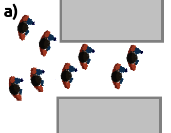
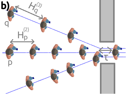
Figure 1: (a) Sketch of the ‘zipper effect’ proposed by Hoogendoorn and Daamen [2]. (b) Sketch of the situation contemplated in our model, in the case of $n=3$ lines. The pedestrians’ minimal headways $H_{p}^{(k)}$ are enlarged for clarity.

4 Correlations between successive time gaps

Using the class of simple models introduced in the previous section, we now enquire into the ‘ingredients’ that give rise to the empirically observed alternation between short time gaps and longer ones, i.e., $\mathcal{C}_{1}<0$.

4.1 Single-file model

First consider a situation with a single line, $n=1$. In this case, assuming congestion, time gaps $\tau_{p}$ coincide with the headways $H_{p}$. Can a heterogeneous distribution of headways then give rise to anticorrelations, $\mathcal{C}_{1}<0$?

At first sight, it is reasonable to assume that the headway $H_{p}$ depends mostly on the intrinsic characteristics of pedestrian $p$. As pedestrians generally arrived in random order in the experiments, the headways of successive pedestrians, $H_{p}$ and $H_{p+1}$, are independent random variables, whence $\left\langle H_{p+1}H_{p}\right\rangle=\left\langle H_{p+1}\right\rangle\left\langle H_{p}\right\rangle=\left\langle H_{p}\right\rangle^{2}$. It immediately follows that $\mathcal{C}_{1}=0$; there is no correlation in this scenario.

Considering the problem in more detail, one realises that, since $H_{p+1}$ is the spacing between pedestrians $p$ and $p+1$, it may actually depend on the morphologies of both agents, e.g., their sizes $S_{p}$ and $S_{p+1}$, because bigger people take more space. Accordingly, $H_{p+1}$ should grow monotonically with $S_{p}$ and with $S_{p+1}$. This renders $H_{p}$ and $H_{p+1}$ positively correlated, because both grow monotonically with $S_{p}$, while $S_{p-1}$ and $S_{p+1}$ are independent. Hence, one expects $\mathcal{C}_{1}>0$, contrary to experimental results.

Consequently, the single-file model is unable to account for the observed anticorrelations. This is consistent with the absence of anticorrelations in some empirical situations in which pedestrians tended to line up ahead of the door [10].

Before we turn to multiple-lane models, a few words should be said about the non-congested case, even though it is less relevant for the considered experiments [2, 5, 9, 10]. In that case, anticorrelations may be obtained if the pedestrians’ walking velocities are not uniform and overtaking is not allowed. Indeed, the interval ahead of particularly slow pedestrians will grow with time, whereas the spacing with the pedestrian just behind them will shrink, and vice versa. Let us mention that anticorrelations were also reported in a single-lane car traffic model in which the driver’s velocity adjusted not only to the gap in front of it ($p$), but also to the previous one $(p-1)$, but such anticorrelations were not observed empirically when single road-lanes were considered [27].

4.2 Theoretical results for the two-lane model

Having discarded the ability of single-file models to capture empirical observations in congested situations, we turn to a scenario with $n=2$ non-interacting lanes. Let us recall that, ahead of the congested bottleneck, pedestrians on both lanes ($k\in\left\{1,2\right\}$) walk at a constant velocity, with spacings $H_{p}^{(k)}$ drawn from a random distribution $p_{H}$ that is assumed independent of the lane $k$. Somewhat counterintuitively, we will show on the basis of a probabilistic reasoning that this simple model of independent lanes already gives rise to anticorrelated time gaps ($\mathcal{C}_{1}<0$).

Without loss of generality, we can suppose that the $p$-th person to egress comes from lane 1. Let $P(\text{Neal}^{(k)},\,\tau)$ be the joint probability that (i) the next agent to leave the room (called Neal) comes from lane $k$ and (ii) the time gap before this upcoming egress is equal to $\tau$. To start with, consider $P(\text{Neal}^{(1)},\,\tau)$. The next egress originates from lane 1 if the next agent on lane 2 (called Neal⁽²⁾) stands behind the cross-hatched region in Fig. 2a, of length $\tau$. Supposing that Neal⁽²⁾’s headway is $H^{(2)}=h\geqslant\tau$, the probability to find him out of the hatched region is $\frac{h-\tau}{h}$ (recall that the files are independent). To conclude, we need to estimate the probability to find such a headway $h$ at the door level. There, a subtlety arises. Indeed, this probability is not $p_{H}\left(h\right)$, but $\frac{h}{\left\langle h\right\rangle}p_{H}\left(h\right)$, because longer headways are encountered more frequently. Bearing in mind this subtlety, the probability that Neal comes from line 1 reads

$$\int_{\tau}^{\infty}\frac{h-\tau}{h}\frac{h}{\left\langle h\right\rangle}p_{H}\left(h\right)dh=\int_{\tau}^{\infty}\frac{h-\tau}{\left\langle h\right\rangle}p_{H}(h)dh.$$

Therefore,

$$P\left(\text{Neal}^{(1)},\tau\right)=p_{H}\left(\tau\right)\mathcal{I}(\tau),$$ (1)

where $\mathcal{I}(\tau)\equiv\int_{\tau}^{\infty}\frac{h-\tau}{\langle h\rangle}p_{H}\left(h\right)dh=\int_{\tau}^{\infty}\frac{P(H>h)}{\langle h\rangle}dh$, with $P(H>h)$ the complementary cumulative distribution function (ccdf) of $p_{H}$.

In the alternative case, sketched in Fig. 2b, Neal⁽²⁾ egresses first. This case will occur if Neal⁽¹⁾’s headway is larger than $\tau$. Thus, it happens with probability $P(H>\tau)$. We are then left with the calculation of the probability to find Neal⁽²⁾ at a distance $\tau$ ahead of the door. Supposing that Neal⁽²⁾’s headway is $h\geqslant\tau$, this probability is simply $1/h$, because the doorway can intersect Neal⁽²⁾’s headway anywhere, owing to the independence between lines. Recalling the aforementioned subtlety, we arrive at

$$P\left(\text{Neal}^{(2)},\tau\right) = P\left(H>\tau\right)\int_{\tau}^{\infty}\frac{1}{h}\frac{h}{\left\langle h\right\rangle}p_{H}\left(h\right)dh$$ (2)

$$= P\left(H>\tau\right)\frac{P\left(H>\tau\right)}{\left\langle h\right\rangle}.$$

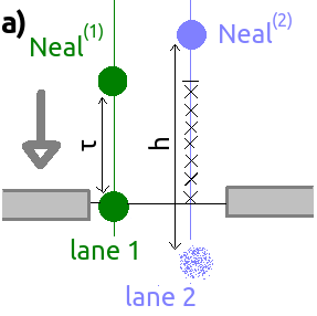
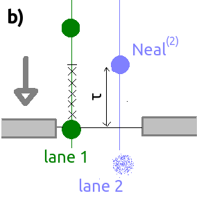
Figure 2: Sketches of the situations in which the next agent to cross the doorway (Neal) is (a) $\mathrm{Neal}^{(1)}$ and (b) $\mathrm{Neal}^{(2)}$. The next time gap is denoted by $\tau$.

Equations 1-2 express the probabilities to find a time gap $\tau_{p}$, if we only know that the last person who egressed came from lane 1. In order to evaluate the correlator $\mathcal{C}_{1},$ we also need to estimate $\tau_{p+1}$, i.e., to consider not only the agent who egresses next (Neal), but also the second next agent to leave, whom we name Seal. The notations deserve a remark: $\tau_{p+1}$ is the time gap measured just after $\tau_{p}$, regardless of the line from which Seal comes. That being said, the derivation of the joint probabilities $P\left(\text{Neal}{}^{(k)},\,\tau_{p},\,\text{Seal}{}^{(k^{\prime})},\,\tau_{p+1}\right)$, i.e., Neal comes from line $k$ and egresses after $\tau_{p}$, followed after $\tau_{p+1}$ by someone from line $k^{\prime}$, is very similar to the derivation detailed above for $\tau_{p}$ and leads to the following expressions,

$$P\left(\text{Neal}^{(1)},\,\tau_{p},\,\text{Seal}^{(1)},\,\tau_{p+1}\right)=p_{H}\left(\tau_{p}\right)\,p_{H}\left(\tau_{p+1}\right)\mathcal{I}\left(\tau_{p}+\tau_{p+1}\right)$$ (3)

$$P\left(\text{Neal}^{(1)},\,\tau_{p},\,\text{Seal}^{(2)},\,\tau_{p+1}\right)=p_{H}\left(\tau_{p}\right)\,P\left(H>\tau_{p+1}\right)\frac{P\left(H>\tau_{p}+\tau_{p+1}\right)}{\left\langle h\right\rangle}$$

$$P\left(\text{Neal}^{(2)},\,\tau_{p},\,\text{Seal}^{(1)},\,\tau_{p+1}\right)=p_{H}\left(\tau_{p}+\tau_{p+1}\right)\frac{P\left(H>\tau_{p}\right)}{\left\langle h\right\rangle}P\left(H>\tau_{p+1}\right)$$

$$P\left(\text{Neal}^{(2)},\,\tau_{p},\,\text{Seal}^{(2)},\,\tau_{p+1}\right)=P\left(H>\tau_{p}+\tau_{p+1}\right)\frac{P\left(H>\tau_{p}\right)}{\left\langle h\right\rangle}p_{H}\left(\tau_{p+1}\right).$$

Finally, these two-point probabilities are inserted into the time gap correlator, viz., $\mathcal{C}_{j}=\left\langle\delta\tau_{p}\delta\tau_{p+1}\right\rangle/\left\langle\delta\tau_{p}^{2}\right\rangle$, where

$$\left\langle\delta\tau_{p}\delta\tau_{p+1}\right\rangle=\iint_{0}^{\infty}(\tau_{p}-\bar{\tau})(\tau_{p+1}-\bar{\tau})\sum_{k,k^{\prime}=1,2}P\left(\text{Neal}^{(k)},\tau_{p},\text{Seal}^{(k^{\prime})},\tau_{p+1}\right)d\tau_{p}d\tau_{p+1}.$$ (4)

Here, the average time gap $\bar{\tau}$ obeys $\bar{\tau}=\langle h\rangle/2$ and the fluctuation $\delta\tau_{p}$ is defined as $\tau_{p}-\bar{\tau}$.

4.3 Evaluation of the correlator for specific headway distributions

Unfortunately, Eq. 4 is complex and the sign of $\mathcal{C}_{1}$ does not immediately transpire from its inspection. Therefore, we will now focus on specific headway distributions, which will simplify the formulae and allow us to test them against simulations of the model.

To start with a simple, but enlightening, example, we assume that headways are constant, i.e., $p_{H}\left(h\right)=\delta\left(h-\bar{h}\right)$. This comes down to studying a perfect zipper in which two regularly ordered lines intercalate with a random offset. In this case, $\bar{\tau}=\bar{h}/2$ and Eqs 3-4 yield

$$\left\langle\delta\tau_{p}^{2}\right\rangle=\frac{\bar{h}^{2}}{12}\text{ and }\left\langle\delta\tau_{p}\delta\tau_{p+1}\right\rangle=\frac{-\bar{h}^{2}}{12}.$$

It follows that $\mathcal{C}_{1}=-1$: Successive time gaps are thus anticorrelated, despite the independence of the lines. There is an intuitive explanation to this observation. Consider an interval between pedestrians in line 1. Because of the random offset between the lines, a pedestrian in line 2 generally splits this interval into a small section and a large one. Since spacings are equal in the two lines, these small and large intervals alternate cyclically, thus generating anticorrelations.

This reasoning hinges on the regular ordering of pedestrians on both lanes. What will remain of it, should the flow be more disordered and pedestrians unequally spaced? To test this more realistic scenario, we consider Gaussian distributions of headways $p_{H}(h)=\left(\delta h\sqrt{2\pi}\right)^{-1}\exp\left[\frac{\left(h-\bar{h}\right)^{2}}{2\delta h^{2}}\right]$, where $\bar{h}=1$ is the mean, and the standard deviation $\delta h$ will be varied to study the influence of the level of disorder. In practice, it will remain small enough for occurrences of $h<0$ to be negligible (in the numerical simulations, negative values of $h$ are shifted to zero). With such Gaussian distributions, explicit analytical formulae can be obtained for the two-point probabilities of Eqs. 3, by inserting the following equalities,

$$P\left(H>h\right)=\frac{1}{2}\mathrm{erfc}\left(\frac{h-\bar{h}}{\delta h\sqrt{2}}\right),\text{ and}$$

$$\mathcal{I}(\tau)=\frac{\delta h^{2}}{\bar{h}}p_{H}(\tau)+\frac{\bar{h}-\tau}{2\bar{h}}\mathrm{erfc}\left(\frac{\tau-\bar{h}}{\delta h\sqrt{2}}\right),$$

where $\mathrm{erfc}$ is the complementary error function. We then rely on numerical integration to evaluate the correlator of Eq. 4. The correlations $\mathcal{C}_{1}$ resulting from this integration accurately match the results of direct numerical simulations of the model for small $\delta h$, as evidenced in Fig 3(left). For larger $\delta h$, the truncation of of $p_{H}$ to positive $h$ in the numerics causes minor differences. Most importantly, we see that $\mathcal{C}_{1}$ is significantly negative not only for vanishing $\delta h$ (almost equal spacings), but also when the flow is entirely disordered, with a rather broad distribution of headways ($\delta h/\bar{h}>\nicefrac{{1}}{{2}}$). We have checked that this also holds if the headway distributions differ between the two pedestrian lines (i.e., if their parameters $\bar{h}$ or $\delta h$ differ). To rephrase this noteworthy result, there tends to be an alternation between short time gaps and longer ones even if pedestrians are not regularly spaced and the lines do not interact.

As a corollary, anticorrelations ($\mathcal{C}_{1}<0$) bring no evidence of a zipper-like intercalation of lines imposed by the narrowness of the bottleneck .

4.4 Effect of extensions of the model

Admittedly, the simple model presented above does not account for all observed features. For instance, the experiments of [10] unveiled a general alternation in the incident directions of egressing pedestrians, i.e., between people coming from the left and from the right. This feature can be enforced in the model by making $\mathrm{Neal}^{(1)}$ wait for $\mathrm{Neal}^{(2)}$ to exit if the last egress was from lane 1; then, $\mathrm{Neal}^{(1)}$ egresses immediately after $\mathrm{Neal}^{(2)}$. This systematic alternation between lines brings our model closer to that of Hoogendoorn and Daamen [2], in which headways were constrained by the impossibility of cross-line overtaking inside the bottleneck. Numerical simulations, represented by cyan stars on Fig. 3(left), show that this new constraint further enhances the anticorrelations, that is, make $\mathcal{C}_{1}$ more negative. This is easily understood: All scenarios $\left(\text{Neal}{}^{(1)},\,\tau_{p},\,\text{Seal}{}^{(1)},\,\tau_{p+1}\right)$ in the previous model turn into scenarios with a longer $\tau_{p}$ and $\tau_{p+1}=0$.

Stronger interactions between lines are expected if the door is so narrow that pedestrians can only pass one by one, which means that the two lines effectively merge at the entrance of the bottleneck. This is incorporated into our model by making pedestrian $p$ (on lane $k$) wait at a distance $H_{p}^{(k)}$ ahead of the door whenever somebody from the other line is currently passing through the door. The next agent to egress is the one that stands closer to the door and the duration of his or her passage is equal to this distance to the door (recall that $v=1$). It turns out that this one-by-one passage rule totally suppresses the time-gap anticorrelations (numerical data not shown); this is due to the fact that agents on lane 2 no longer split the headways on lane 1. As one can imagine, prescribing a systematic alternation between lines, as in a bona fide zipper, does not restore the anticorrelations.

On the contrary, larger doors can accommodate multiple virtually independent lanes. Restoring the independence between lanes, we compute the variations of $\mathcal{C}_{1}$ with the number of lanes $n$. The results are plotted in Fig. 3(right) and prove that anticorrelations persist for $n\geqslant 2$, even though they weaken with increasing $n$.

To summarise the results of this section, within the rather general framework of our model, time-gap anticorrelations emerge if several pedestrians (from distinct lines or directions) can cross the door within a very short interval, as compared to the headways. Accordingly, we speculate that anticorrelations would be suppressed in any experiment with a very narrow door, only allowing one pedestrian to pass at a time.

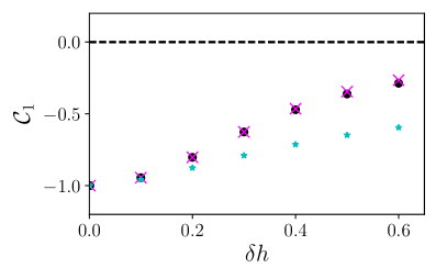
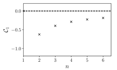
Figure 3: Correlations between successive time gaps, $\mathcal{C}_{1}=\frac{\left\langle\delta\tau_{j}\delta\tau_{j+1}\right\rangle}{\left\langle\delta\tau_{j}^{2}\right\rangle}$, for Gaussian distributions of minimal headways with unit mean and standard deviation $\delta h$. (Left) Dependence of $\mathcal{C}_{1}$ on $\delta h$ for two independent lanes of pedestrians. Black dots were obtained with the theoretical expression of Eq. 4; pink crosses are simulation results. Cyan stars correspond to simulations of the model enforcing an alternation between lines. (Right) Variations of $\mathcal{C}_{1}$ with the number $n$ of (independent) lanes, for $\delta h=0.3$.

5 Distribution of burst sizes

When the time-series of exits is inspected at a more global scale than that of individual time gaps, clusters of uninterrupted escapes, called bursts, become apparent in competitive conditions [13, 8, 10]. In practice, a more precise criterion is required to delimit bursts. Usually, one sets an arbitrary upper bound $\tau^{b}$ on the admissible time-gaps within a burst. A similar criterion can be applied to identify bursts in more ordered flows.

In Section 2, we recalled that, regardless of the precise value $\tau^{b}$, the competitiveness of the crowd and the experimental settings, pedestrian experiments consistently measured exponentially distributed burst sizes $S$, at large $S$ [9, 10]. The model introduced in Section 3 and all variants discussed so far are no exception to this rule, as confirmed by the data shown in Fig 4. Is the exponential pdf of burst sizes then a truly universal feature of bottleneck flows? In the following, after examining the origin of this feature, we contemplate situations which lead to heavier-than-exponential distributions of $S$.

5.1 A Poisson process in the congested case

As long as the probability that a burst is interrupted before the passage of a new agent takes a constant value $p_{c}$, with $0<p_{c}<1$, the egress will be a Poisson process of rate $p_{c}$, which implies $p(S)\approx p_{c}e^{-p_{c}S}$ for $S\rightarrow\infty$. In a granular hopper flow, $p_{c}$ is the clogging probability per grain [18]. In our pedestrian flow models, $p_{c}$ simply represents the probability to find a time gap larger than $\tau^{b}$, $p_{c}=P\left(\tau>\tau^{b}\right)$. Despite the presence of short-term correlations $\mathcal{C}_{p}$ (which undermine the argument), evaluating $p_{c}$ in this way with the help of Eqs. 1-2 results in very good fits to simulation results, as shown in Fig. 4, provided that $\tau_{b}$ is sufficiently large. For smaller $\tau_{b}$, $p(S)$ seems to still decay exponentially at large $S$, but the correlations between successive time gaps induce deviations from the fit based on $p_{c}$.

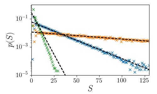
Figure 4: Distributions of burst sizes $S$ obtained in simulations of $n=2$ non-interacting lanes with Gaussian-distributed headways (mean $\bar{h}=1$, standard deviation $\delta h=0.3$), with the burst criterion set to $\tau^{b}=0.7$ (green crosses), 1 (blue crosses), 1.2 (orange crosses). The dashed lines are the exponential fits $p(S)=p_{c}e^{-p_{c}S}$, where $p_{c}$ is evaluated using Eqs. 1-2. Note the semi-logarithmic axes.

5.2 Possibility of anomalous statistics

Despite all apparences to the contrary, we argue that exponential burst size distributions are not universal and that power-law distributions can arise in particular situations close to congestion. Extending the model presented in Section 3 to non-congested situations, we denote by $X_{p}^{(k)}(t)\leqslant 0$ the position of pedestrian $p$ on lane $k$ at time $t$, with the origin at the door. The agent’s actual headway

$$\delta X_{p}^{(k)}(t)\equiv X_{p-1}^{(k)}(t)-X_{p}^{(k)}(t)$$

is always larger than the minimal headway $H_{p}^{(k)}$, viz., $\delta X_{p}^{(k)}(t)\geqslant H_{p}^{(k)}$. Both $H_{p}^{(k)}$ and the initial headway $\delta X_{p}^{(k)}(0)$ are random variables drawn once and for all from distributions that are identical for all lanes (i.e., that do not depend on $k\in\left\{1,\ldots,n\right\}$). To illustrate our findings, we will choose Gaussian distributions, with respective means $\left\langle H_{p}^{(k)}\right\rangle=\overline{H}$ and $\left\langle\delta X_{p}^{(k)}(0)\right\rangle=n\,\overline{\delta X}$, where $\overline{\delta X}$ is the average initial spacing between pedestrians, all lanes combined.

The door is supposed narrow, so that only one agent (Neal) can pass at a time, as in the variant introduced in Section 4.4. We remind the reader that during Neal’s passage, his competitors $p$ on lane $k$ cannot move closer than a distance $H_{p}^{(k)}$ to the door, which may force them to halt and may reduce the headways $\delta X_{p^{\prime}}^{(k)}(t)$ of the people behind. As soon as Neal has left, the agent closest to the door can egress.

Quite interestingly, numerical simulations show that for a (limited) range of parameters this model yields distributions of burst sizes $p(S)$ whose tails are heavier than exponential and are well fitted by power laws (see Fig. 5).

5.3 Delay accumulation and power-law statistics

To clarify the origin of these anomalous statistics, a theoretical analysis of the model is helpful. The analysis is simplified by focusing on the line that results from the merger of the $n$ lines at the door. Therefore, we label pedestrians according to their order of egress and drop the $(k)$ superscripts referring to the lane from which they come. With this new labelling, the $\delta X_{p}(t)$’s are algebraic distances and may be positive or negative. Besides, the sequence of time gaps between egresses is $\tau_{1},\ldots,\tau_{N}$ and pedestrians $(p-1)$ and $p$ belong to the same burst if $\tau_{p}\leqslant\tau^{b}$.

If the bottleneck is not congested, the time gaps $\tau_{p}$ need not coincide with the minimal headways $H_{p}$, but result from the shrinkage of the interpedestrian spacings due to halts. We are thus led to study the propagation of halts (or <<jams>>). Let $D_{p}$ be the cumulative halting time (delay) of agent $p$ from start $(t=0)$ to egress $(t=t_{p})$. To find an iterative relation between $D_{p}$ and $D_{p-1}$, we consider a fictional situation in which pedestrians just walk at constant velocity ($v=1$), without halts; this can be realised by setting $H_{p}=0$ for all agents $p$, all other things being equal. In the fictional scenario, referred to by prime superscripts, spacings are preserved, viz.,

$$\delta X_{p}^{\prime}(t)=\delta X_{p}^{\prime}(0)=\delta X_{p}(0),$$

Recalling that $X_{p}(t_{p})=0$, we remark that the delay $D_{p}$ in the actual model coincides with $X_{p}^{\prime}(t_{p})$, so that

$$D_{p} = X_{p}^{\prime}(t_{p})$$

$$= X_{p}^{\prime}(t_{p-1})+t_{p}-t_{p-1}$$

$$= X_{p-1}^{\prime}(t_{p-1})-\delta X_{p}(0)+\tau_{p}$$

$$= D_{p-1}-\delta X_{p}(0)+\tau_{p}.$$

Now, $D_{p}>0$ means that agent $p$ has halted due to congestion, which reduced his or her actual headway to $H_{p}$, so $\tau_{p}=H_{p}$. The alternative case, $D_{p}=0$, corresponds to only free walk for agent $p$ and implies $\tau_{p}=-D_{p-1}+\delta X_{p}(0)$. In Table 1, we sum up the coupled equations of evolution of $\tau_{p}$ and $D_{p}$ that directly follow from these considerations.

	If $\boldsymbol{D_{p-1}>H_{p}-\delta X_{p}(0)}$ (congestion),	Otherwise (free walk),
$\tau_{p}=$	$H_{p}$	$-D_{p-1}+\delta X_{p}(0)$
$D_{p}=$	$D_{p-1}+H_{p}-\delta X_{p}(0)$	0

Table 1: Iterative relations governing the coupled evolutions of time gaps $\tau_{p}$ and cumulative delays $D_{p}$.

Since $H_{p}$ and $\delta X_{p}(0)$ are random variables with mean values $\overline{H}$ and $\overline{\delta X}$, respectively, $D_{p}$ performs a one-dimensional random walk in “time” $p$ with a bias $\overline{H}-\overline{\delta X}$, close to the absorbing boundary $0^{+}$. Depending on the bias, different flow regimes are expected. (i) If the bias is strongly positive, i.e., $\overline{\delta X}\ll\overline{H}$ , congestion is expected for the greatest part of time. (ii) For $\overline{H}\simeq\overline{\delta X}$, $D_{p}$ performs a virtually unbiased random walk. The survival times $S_{\mathrm{cong}}$ of the congested phases $D_{p}>0$ are thus distributed according to $p(S_{\mathrm{cong}})\sim S_{\mathrm{cong}}^{-\frac{3}{2}}$. (iii) For $\overline{\delta X}\gg\overline{H}$, free walk prevails, and the distribution of congested durations $S_{\mathrm{cong}}$ will decay quickly at large time scales, due to the downward drift of $D_{p}$, of magnitude $\overline{H}-\overline{\delta X}$.

In Section 5.1, we saw that bursts within a congested phase do not display anomalous (heavy-tailed) statistics. Therefore, to have a chance to observe anomalous statistics, bursts must not end during these phases. Thus, $P\left(H>\tau^{b}\right)$ must be negligible. With a somewhat sloppy notation, we write this condition $\sup\left(H\right)<\tau^{b}$. At the same time, $\tau^{b}$ must be small enough to separate bursts between subsequent congested phases, viz., $\tau^{b}\leqslant\overline{\delta X}$ (otherwise, bursts would follow a Poisson process dependent on the initial spacings). Under these combined conditions, the burst sizes coincide with the survival times $S_{\mathrm{cong}}$, which are power-law distributed in regime (ii), $\overline{H}\simeq\overline{\delta X}$. Figure 5 shows that, if all these conditions are fulfilled, a power-law distribution of burst sizes with exponent $-\nicefrac{{3}}{{2}}$ is indeed observed.

However, this regime is highly constrained in parameter space, since the inequality $\sup\left(H\right)<\tau^{b}\leqslant\overline{\delta X}$ must be fulfilled at the same time as $\overline{H}\simeq\overline{\delta X}$. In practice, this is only achieved if the minimal headways $H_{p}$ are quite narrowly distributed and $\tau^{b}\simeq\sup\left(H_{p}\right)\simeq\overline{\delta X}$ . Otherwise, $p(S)$ displays a cut-off.

On a more subtle note, it may be remarked that the above reasoning is oblivious to possible correlations in the random walk of $D_{p}$ due to the lane structure of the flow. It discards the fact that, for agents on the same lane, $H_{p}^{(k)}-\delta X_{p}^{(k)}(0)$ is always negative. This fact enhances the likelihood of the interruption of a congested phase every $n$ egresses, which leads to the pdf (and ccdf) oscillations of period $n$ that can be seen in Fig. 5.

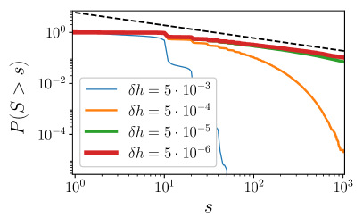
Figure 5: Complementary cumulative distributions $p(S)$ of burst sizes $S$ obtained numerically for Gaussian distributions of minimal headways of mean $\overline{H}=1$ and standard deviation $\delta h$, as indicated in the legend. $n=3$ lanes (left) and $n=10$ lanes (right). The initial distribution of spacings is also Gaussian, with mean value $n(1+10\delta h)$. The burst criterion $\tau^{b}$ was adjusted to be the average between $\overline{H}$ and the mean initial spacing (with all lines combined). The dashed black lines have slopes $\nicefrac{{-1}}{{2}}$, which corresponds to an exponent $\nicefrac{{-3}}{{2}}$ for the pdf.

5.4 Analogy with fibre bundles and depinning problems

There is perhaps a more intuitive way to interpret the distributions of burst sizes $S$. It consists in drawing a parallel with fibre bundle models [28] or depinning models [29]. In these models, the rupture of a fibre, or the motion of a site, destabilises other elements via the redistribution of some positive load $\tau$, which may trigger another rupture. In the mean-field picture, the redistributed load is equally shared among all other elements. To clarify the analogy with our models, we liken the egress of a pedestrian to the rupture of a fibre. In the same way as a broken fibre enhances the probability of subsequent rupture, an egress postpones the end of a burst. The extra time thus given to other agents to exit in the same burst is equal to $\tau=\tau_{p}+\min(\tau_{p+1},\tau^{b})>0$.

Now, it is known that fibre bundle models display cascades of ruptures whose sizes $S$ are power-law distributed close to criticality, with $p(S)\sim S^{-\frac{3}{2}}$ [28]. Farther from the critical point, e.g., when the system is too stable to be entirely destabilised by a single rupture, the power-law distribution is cut-off exponentially. In the light of this analogy, we should not have been surprised to detect a power-law distribution of burst sizes with exponent $3/2$ in the pedestrian model at the transition between a dilute flow and a congested one, provided that the criticality of this transition was not washed out by the disorder in the headways and the finite number of lanes.

6 Conclusions

In summary, we have enquired into the microscopic dynamics of pedestrian flows through a bottleneck, with a strong emphasis on the time gaps $\tau$ between egresses. Our study, based on simple models, sheds light on the mechanisms underlying the experimentally evidenced statistical properties of these time gaps. More precisely, our models show that, contrary to a widespread belief, the anticorrelations between successive time gaps (that is, the alternation between short and long time gaps), which have been reported in various settings, are not a hallmark of a zipper-like intercalation of pedestrian lines. Instead, they naturally emerge whenever the bottleneck is wide enough to allow two or more pedestrians to cross it within a short time interval. Under these conditions, the pedestrian’s headways within a line are split into (generally unequal) sections by the independent passage of another pedestrian, thereby yielding anticorrelations. The minimality of these conditions rationalises the observation of this effect in competitive evacuations as well, where pedestrians did not line up in front of the door. Turning to the second statistical feature, the ubiquitous exponential distributions of burst sizes owe their origin to the constant probability that the lagging egress of a pedestrian marks the end of the burst. Nevertheless, our study unveiled the possibility of anomalous (power-law) statistics if the system is on the brink of congestion and the burst criterion is fine-tuned; the model can then be amalgamated to a fibre bundle. However, this regime only covers a tiny portion of parameter space. It remains to be seen if some vestige of these anomalous statistics can be detected experimentally, in the form of a power law with an exponential cut-off.

Finally, it should be stressed that the mechanisms giving rise to these statistical properties are very general. In fact, they do not rely on any distinctive feature of pedestrian motion. Therefore, we also expect anticorrelations between time gaps to be observed in other types of constricted flows too, such as hopper flows of granular discs, evacuations of mice or multiple-lane vehicular traffic.

References

- [1] Isobe M, Helbing D and Nagatani T 2004 Physical Review E 69 066132
- [2] Hoogendoorn S P and Daamen W 2005 Transportation science 39 147–159
- [3] Kretz T, Grünebohm A and Schreckenberg M 2006 Journal of Statistical Mechanics: Theory and Experiment 2006 P10014
- [4] Nagai R, Fukamachi M and Nagatani T 2006 Physica A: Statistical Mechanics and its Applications 367 449–460
- [5] Seyfried A, Passon O, Steffen B, Boltes M, Rupprecht T and Klingsch W 2009 Transportation Science 43 395–406
- [6] Seyfried A, Steffen B, Winkens A, Rupprecht T, Boltes M and Klingsch W 2009 Empirical data for pedestrian flow through bottlenecks Traffic and Granular Flow 2007 (Springer) pp 189–199
- [7] Liddle J, Seyfried A, Steffen B, Klingsch W, Rupprecht T, Winkens A and Boltes M 2011 arXiv preprint arXiv:1105.1532
- [8] Pastor J M, Garcimartín A, Gago P A, Peralta J P, Martín-Gómez C, Ferrer L M, Maza D, Parisi D R, Pugnaloni L A and Zuriguel I 2015 Physical Review E 92 062817
- [9] Garcimartín A, Parisi D, Pastor J, Martín-Gómez C and Zuriguel I 2016 Journal of Statistical Mechanics: Theory and Experiment 2016 043402
- [10] Nicolas A, Bouzat S and Kuperman M N 2017 Transportation Research Part B: Methodological 99 30–43
- [11] Liddle J, Seyfried A, Klingsch W, Rupprecht T, Schadschneider A and Winkens A 2009 arXiv preprint arXiv:0911.4350
- [12] Helbing D, Farkas I and Vicsek T 2000 Nature 407 487–490
- [13] Zuriguel I, Parisi D R, Hidalgo R C, Lozano C, Janda A, Gago P A, Peralta J P, Ferrer L M, Pugnaloni L A, Clément E et al. 2014 Scientific reports 4
- [14] Helbing D, Johansson A, Mathiesen J, Jensen M H and Hansen A 2006 Physical review letters 97 168001
- [15] Nicolas A, Bouzat S and Kuperman M N 2016 Phys. Rev. E 94(2) 022313
- [16] Janda A, Maza D, Garcimartín A, Kolb E, Lanuza J and Clément E 2009 EPL (Europhysics Letters) 87 24002
- [17] Parisi D and Dorso C 2007 Why ’faster-is-slower’ in evacuation process Pedestrian and Evacuation Dynamics 2005 (Springer) pp 341–346
- [18] Mankoc C, Garcimartín A, Zuriguel I, Maza D and Pugnaloni L A 2009 Physical Review E 80 011309
- [19] Garcimartín A, Pastor J, Ferrer L M, Ramos J, Martín-Gómez C and Zuriguel I 2015 Physical Review E 91 022808
- [20] Lin P, Ma J, Liu T, Ran T, Si Y and Li T 2016 Physica A: Statistical Mechanics and its Applications 452 157–166
- [21] Hoogendoorn S P, Daamen W and Bovy P H 2003 Extracting microscopic pedestrian characteristics from video data Transportation Research Board Annual Meeting pp 1–15
- [22] Al Reda F 2017 Modélisation de mouvement de foules avec contraintes variées Ph.D. thesis Université Paris-Sud
- [23] Zuriguel I, Pugnaloni L A, Garcimartin A and Maza D 2003 Physical Review E 68 030301
- [24] Saraf S and Franklin S V 2011 Physical Review E 83 030301
- [25] Perez G J, Tapang G, Lim M and Saloma C 2002 Physica A: Statistical Mechanics and its Applications 312 609–618
- [26] Masuda T, Nishinari K and Schadschneider A 2014 Cellular automaton approach to arching in two-dimensional granular media Cellular Automata (Springer) pp 310–319
- [27] Eissfeldt N and Wagner P 2003 The European Physical Journal B-Condensed Matter and Complex Systems 33 121–129
- [28] Sornette A and Sornette D 1989 EPL (Europhysics Letters) 9 197
- [29] Fisher D S 1983 Physical Review Letters 50 1486