DEPHASING ASSISTED TRANSPORT
ON A BIOMIMETIC RING STRUCTURE

Abstract

We address two-level systems arranged in ring configurations affected by static disorder. In particular we investigate the role of dephasing in the transport of an excitation along the ring. We compare the efficiency of the transfer process on isotropic rings and on biomimetic rings modelled according to the structure of light-harvesting complexes. Our analysis provides a simple but clear and interesting example of how an interplay between the coherent dynamics of the system and the incoherent action of the environment can enhance the transfer capabilities of disordered lattices.

1 Introduction

Quantum coherent evolution can provide a substantial advantage with respect to classical random walks for the task of transferring energy or information between selected vertices of a graph [1, 2, 3, 4]. The latter, in turn, can be used to model the different parties of a composite system, such as, for example, a communication network or a biological complex [5, 6]. Recent experiments have revealed the presence of quantum coherence in the Exciton Energy Transfer processes (EET) that occur on the photosyntetic membranes of purple bacteria [7, 8, 9]. This observations triggered quite a large amount of research aimed to understanding whether Nature itself is exploiting quantum coherence as a resource in EET, which is well known to be a remarkably efficient biological processes [10, 11, 12, 13, 14, 15, 16]. The understanding of the fundamental mechanism that allows for such efficiency can provide design principles for synthetic photovoltaic devices [17].

Coherence, on the other side, is usually washed away by the unavoidable interaction of the system with the surrounding environment which is therefore expected to detriment the EET efficiency. Recent research, however, showed that there are situations where the presence of a certain amount of decoherence can actually be beneficial for transport [12, 18, 19, 13, 20]. In the presence of static disorder, for example, dephasing can help delocalizing an excitation that would otherwise suffer from Anderson localization. This phenomenon is known as Dephasing Assisted Transport (DAT).[12, 13]

In this paper we investigate excitation transfer on a ring, i.e. $N$-cycle graph, in the presence of disorder and decoherence. We consider $N$-cycles graphs with isotropic and alternate nearest-neighbour coupling. The latter configuration resembles the structure of Light Harvesting complexes of type 1, called LH1 (see Ref.s 21, 22), and 2, LH2 (see Ref. 23) that can be found on the photosynthetic membrane of purple bacteria. The aim of the paper is to provide simple but interesting examples of the possible role of dephasing in transport over disordered $N$-cycle lattices. In particular we show that dephasing can assists transport on both types of rings, when the on-site energies of the cycles are affected by static disorder. We moreover find that alternate couplings do not offer any functional advantage with respect to excitation transfer between two opposite sites of the $N$-cycle.

The paper is organized as follows. In Section 1 we introduce and characterize the ring models and define the the adopted EET efficiency measure. In Section 2 we define the disorder and dephasing and study their relative effects on EET. Section 3 presents the analysis of the conbined effects of disorder and dephasing. The last section is devoted to conclusion and outlook.

2 The model

The quantum system we consider in this paper is a collection of $N$ two-level systems (TLSs) arranged in a circular structure. Each TLS $j$, $j=1,2,\ldots,N$, can be in its ground, $|0\rangle_{j}$, or excited, $|1\rangle_{j}$ state. We restrict our analysis to the relevant single excitation case [24], where only one of the TLSs is excited while the others are all in the ground state. Defined $|j\rangle=\otimes_{n=1}^{N}|\delta_{j,n}\rangle_{n}$, the set $\{|j\rangle\}_{j=1}^{N}$ is a basis for the Hilbert space of considered states. In this basis the system Hamiltonian reads:

$$H=\sum_{j=1}^{N}J(j)(|j+1\rangle\langle j|+|j\rangle\langle j+1|)+\varepsilon(j)|j\rangle\langle j|,$$ (1)

with the condition $|N+1\rangle=|1\rangle$ accounting for the closed boundary conditions. The coefficients $J(j)$ represent the coupling strength between nearest-neighbour sites whereas $\varepsilon(j)$ are the on site energy difference between the ground and excited state of the $j$-th TLS.
In what follows we will study the transfer of the single excitation for two different parametrizations of the ring Hamiltonian $H$. In the first one we consider isotropic couplings $J(j)=J$ and equal on-site energies $\varepsilon(j)=\varepsilon$ (without loss of generality we can set, in this case, $\varepsilon=0$). The Hamiltonian corresponding to this parametrization reduces to:

$$H_{\rm R}=J\sum_{j=1}^{N}|j+1\rangle\langle j|+|j\rangle\langle j+1|.$$ (2)

The second parametrization is chosen as to resemble the configuration of the LH1 complex of purple photosynthetic bacteria (Rhodospirillum rubrum) [22]. This complex is formed by 32 BChl molecules, bound to 16 $\alpha$ and $\beta$ polypeptides as $\alpha\beta(\text{BChl)}_{2}$ subunits organized in a ring geometry. The $\alpha$ and $\beta$ polypeptides of nearest-neighbour subunits are interacting with each other with inter-dimer coupling strength $J_{2}=377\mbox{cm}^{-1}$ whereas the $\alpha\beta$ BChls in the same subunit are coupled with intra-dimer coupling coefficient $J_{1}=600\mbox{cm}^{-1}$. While the on-site energies $\varepsilon_{\alpha}$ and $\varepsilon_{\beta}$ of the LH1 for the $\alpha$ and $\beta$ polypeptides are slighty different ($\varepsilon_{\alpha}/\varepsilon_{\beta}=0.999$), we assume, for the sake of simplicity, $\varepsilon_{\alpha}=\varepsilon_{\beta}$. The Hamiltonian for this biomimetic configuration of the ring can be written as:

$$H_{\rm LH1} =\sum_{j=0}^{N/2}J_{1}(|2j+2\rangle\langle 2j+1|+|2j+1\rangle\langle 2j+2|)$$

$$\hskip 56.9055pt+\sum_{j=1}^{N/2}J_{2}(|2j+1\rangle\langle 2j|+|2j\rangle\langle 2j+1|),$$ (3)

where we have omitted the dynamically irrelevant on-site energies $\varepsilon_{j}$, and $N=32$. As to allow for a direct comparison between the two ring configurations, we will set for the system described by (2) $N=32$ and $J=(J_{1}+J_{2})/2$.

The spectra of $H_{\rm R}$ and $H_{\rm LH1}$ can both be analytically computed. For the isotropic case, the eigenvectors of $H_{\rm R}$ are given by the Fourier basis

$$|e_{k}^{\rm R}\rangle =\frac{1}{\sqrt{N}}\sum_{j=1}^{N}e^{i\frac{2\pi k}{N}j}|j\rangle,\quad k=1,2,\ldots,N$$ (4)

with corresponding eigenvalues $e_{k}^{\rm R}=-2J\cos\left(\frac{2\pi k}{N}\right)$. To solve the eigenvalue/vector problem for the LH1 dimerized Hamiltonian (3), it is instead expedient to use a relabelling of the $j$-th TLS of the ring with the couple $\left(n=\lfloor j/2\rfloor,s=(j\mod 2)+1\right)$ and to define the Fourier basis

$$|k,s\rangle=\frac{1}{\sqrt{K}}\sum_{n=0}^{K-1}e^{i\frac{2\pi}{K}kn}|n,s\rangle.$$ (5)

The Hamiltonian (3) assumes, in this basis, a block-diagonal form whose $2\times 2$ matrices on the diagonal are:

$$h_{k}=\left(\begin{array}[]{c c}0&J_{1}+e^{-i\alpha_{k}}J_{2}\\ J_{1}+e^{i\alpha_{k}}J_{2}&0\end{array}\right),$$

with $\alpha_{k}=2\pi k/K$ and $K=N/2$; each $h_{k}$ has eigenvalues $\pm e_{k}^{\rm LH}$, with $e_{k}^{\rm LH}=J_{2}\sqrt{\beta^{2}+1+2\beta\cos\alpha_{k}}$, where $\beta=J_{1}/J_{2}$ indicates the degree of dimerization and is diagonalized by the transformation

$$U_{k}=\frac{1}{\sqrt{2}}\left(\begin{array}[]{c c}\eta_{k}&-\eta_{k}\\ 1&1\end{array}\right),$$

with $\eta_{k}=(\beta+e^{-i\alpha_{k}})/e_{k}^{\rm LH}$.

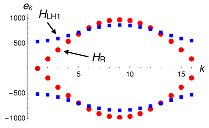
Figure 1: The spectra of $H_{\rm R}$ (circles) and $H_{\rm LH1}$ (squares) for the parametrization given in the main text.

Figure 1 shows the spectra of the isotropic (circles) and the biomimetic, or dimerized, (squares) rings: in both cases the spectra have two bands. In the presence of alternate couplings $J_{1},J_{2}$, however, the spectrum shows an energy gap $2J_{2}\sqrt{1+\beta^{2}}$, i.e. directly proportional to the degree of dimerization $\beta$. In order to study the transport through the rings we assume that the excitation is initially localized on the TLS $j=1$, namely $|\psi(0)\rangle=|1\rangle$, and evaluate the probability of finding the excitation at the opposite site $j=17$ at time $t$, i.e. $|\langle 17|\psi(t)\rangle|^{2}\stackrel{{\scriptstyle\text{def}}}{{\equiv}}p_{17}(t)$. The result is shown in figure 2. Due to the symmetric couplings of site $j=1$ to its nearest-neighbours, in the case of an isotropic ring the initial condition separates in two wavefronts of equal amplitudes that propagate at the same rate along the ring in opposite directions and arrive “simultaneously” at the opposite site. In the presence of alternate couplings, the broken symmetry is made evident by the two separated peaks (around $Jt=22$ and $Jt=28$), formed by the two wavefronts that, in this case, are not symmetrically evolving.

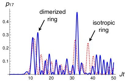
Figure 2: The transfer probability $p_{17}(t)=|\langle 17|\psi^{\rm R/LH}\rangle{(t)}|^{2}$ as a function of time, with $|\psi^{\rm R/LH}(t)\rangle=e^{-itH_{\rm R}/H_{\rm LH}}|1\rangle$. Dotted (red) line: isotropic ring with $J=(J_{1}+J_{2})/2$. Solid (blue) line: dimerized ring. $J_{1}=600$, $J_{2}=377$, $J=(J_{1}+J_{2})/2$.

In the case of the biomimetic configuration it is therefore not immediate to quantify the transfer efficiency. Following Ref. 13 we introduce an extra site, that we indicate by $|s\rangle$, that acts as a sink to which the population is irreversibly transferred from site $N/2+1$. Once defined the operator $S=|s\rangle\langle N/2+1|$, the transfer to the sink is modelled by a Lindblad term

$$\mathcal{L}_{\rm sink}[\rho] =\Gamma\left[2S\rho S^{\dagger}-\{S^{\dagger}S,\rho\}\right].$$ (6)

The efficiency of the transfer at a given time $t$ will be defined as the occupation probability of the sink site, i.e.

$$p_{\rm sink}(t)=\langle s|\rho(t)|s\rangle,$$ (7)

where $\rho(t)$ is the solution of the Lindblad master equation

$$\frac{d}{dt}\rho(t)=-i[H_{\rm R/LH},\rho(t)]+\mathcal{L}_{\rm sink}[\rho(t)],$$ (8)

with initial condition $\rho(0)=|1\rangle\langle 1|$. We now analyse the dependence of $p_{\rm sink}(t)$ on the parameter $\Gamma$ looking for an optimal configuration. We remark that this measure is equivalent to other transfer measures (see, for example Ref. 13). As the inset of figure 3 shows, the population of the sink at a time $Jt=50$, the transfer rate is optimal when it assumes values in a neighbourhood of $J$. As one may expect, for values of $\Gamma$ much smaller than the (average) coupling strength between the ring sites, the transfer to the sink site much slower than the ring evolution; on the other side, for $\Gamma$ larger than the excitation exchange average rate, the evolution of the site $j=17$ gets “frozen” because of a quantum-Zeno-like effect [25]. In what follows, we therefore adopt the optimal value $\Gamma=2J$. In figure 3 we show an example of the population of the sink as a function of time for $\Gamma/J=2$ for the isotropic and biomimetic ring configurations. We observe that the sink populations for the two ring configurations are comparable, even though the dimerized ring shows a slightly reduced transfer capability.

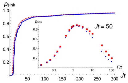
Figure 3: The sink population $p_{\rm sink}(t)$ as a function of $Jt$ for the isotropic (red, dashed line) and the dimerized (blue solid line) ring. Inset: the sink population at fixed time $Jt=50$ for the isotropic (red squares) and the biomimetic (blue circles) configurations as a function of $\Gamma/J$. For both configurations the optimal sink rate $\Gamma$ is achieved for $\Gamma/J\approx 2$.

3 The effect of disorder and dephasing

The models presented in the previous section are idealized. Any physical realization of the lattice will in fact be subjected to different kinds of imperfections; for instance, the on site energies of the TLSs composing the system might differ from each other or the interaction between nearest neighbour can vary from site to site, e.g. because of different relative distances. Moreover, the system can be affected by noise sources: if the TLSs are embedded in a scaffold, they will experience effects due, e.g. to the vibrations (phonons) of the latter. The specific kind of disorder and noise influencing the dynamics of the system, however, is very dependent on the particular physical realization. In the case of the light harvesting complex LH1 our dimerized model is inspired by, even the mere structure of the complex is still debated. [26, 27, 28]

In this work we adopt a paradigmatic approach and consider static (i.e. time-independent) randomly distributed disorder affecting only the on-site energies of the ring Hamiltonians (2) and (3). Such disorder is represented by a diagonal term

$$H_{\rm dis}^{\sigma}(\vec{\mathcal{E}})=\operatorname{\hbox{diag}}\left(\mathcal{E}_{1},\mathcal{E}_{2},\ldots,\mathcal{E}_{N}\right),$$ (9)

with $\mathcal{E}_{i}$ independent random variables with zero-mean Gaussian distribution with standard deviation $\sigma$, quantifying the amount of disorder. Disorder introduces a random on-site energy detuning between different sites of the ring which tends to localize the eigenstates of the Hamiltonian. This results in a localization of the evolving state within a typical $\sigma$-dependent localization length (Anderson localization [29, 30]) thus reducing the transfer capabilities of the ring [31].

We now quantify the effect of disorder on the transfer process for a fixed value of $\sigma$. In order to make the results independent of the particular realization of the diagonal term (9), we need to simulate the evolution of the system for a large number $M$ of realizations of the stochastic Hamiltonian part. For each realization $H_{\rm dis}(\vec{\varepsilon}_{m})$ we numerically determine the states $\rho_{m}(t),\ m=1,2,\ldots,M$, as the solution of (12) with $\vec{\varepsilon}=\vec{\varepsilon}_{m}$. The transfer efficiency is defined as:

$$\bar{p}_{\rm sink}^{M}(t)=\frac{1}{M}\sum_{m=1}^{M}\langle s|\rho_{m}(t)|s\rangle.$$ (10)

In figure 4(a) we plot the sink population as a function of the ratio $\sigma/J$ for the isotropic and dimerized ring configurations at a time $Jt=100$. The transfer efficiency, computed over an average of $M=50$ random realizations is a decreasing function of $\sigma$, as expected. We point out that the transport over the dimerized ring is much more affected by disorder than in the case of a ring with isotropic couplings.

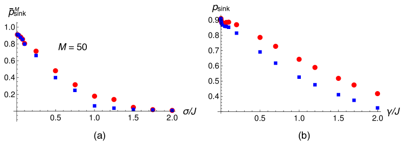
Figure 4: (a) The transfer efficiency $\bar{p}_{\rm sink}^{M}(t)$ as defined in (10) at time $Jt=100$ as a function of the ratio $\sigma/J$ for the isotropic and dimerized rings and $M=50$. (b) The transfer efficiency (7) in the presence of dephasing alone as a function of $\gamma/J$. In both frames red circles refer to the isotropic ring whereas blue squares refer to the biomimetic configuration.

The interaction of the system with a very large number of degrees of freedom, i.e. an environment, can induce different effects to the system. As mentioned above the vibration of the trapping lattice or, in the case of LH1, the proteic scaffold surrounding the TLSs, however, can change their relative positions thus making the coupling coefficients time-dependent. In this case the coupling coefficients would be functions of time. Another noise source is the interaction of each TLS with its local environment, leading to fluctuations of its on-site energy. Such fluctuations lead to a broadening of the line-shape spectrum of each TLS [32, 33, 34]. Following Ref. 35, here we adopt a Markovian effective description of the interaction of each TLS with its local environment and consider only pure dephasing local terms. Such effective description can be seen as a coarse-graining of the stochastic random fluctuations of the on site energies and results in the suppression of the phase coherences of any superposition state of the system. The dephasing process can be modelled by the Lindblad-form super-operator:

$$\mathcal{L}_{\rm deph}[\rho] =\gamma\sum_{j=1}^{N}2|j\rangle\langle j|\rho|j\rangle\langle j|-\left\{|j\rangle\langle j|,\rho\right\},$$ (11)

where we considered the dephasing rates equal for all sites. Figure 4(b) shows the transfer efficiency (7) at the same time $Jt=100$ as in figure 4(a) for the isotropic and dimerized rings in the absence of disorder ($\sigma=0$) as a function of the ratio $\gamma/J$. The loss of coherences detriments the transfer process by making it much slower. It is easy to show, moreover, that in the limit $\gamma\gg J$ the excitation spreads on the lattice at a rate that is close to a purely diffusive process. However, for long times pure dephasing leads to a higher population of the sink site w.r.t. the purely coherent evolution. In figure 5 we show an example of the effect of dephasing for both a small and a large value of the ratio $\gamma/J$. We observe that dephasing affects the excitation transfer to the sink more in the case of a biomimetic ring configuration than in the case of a isotropic ring and such difference becomes more pronounced for larger values of $\gamma$ w.r.t. $J$.

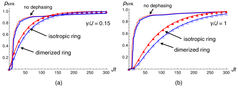
Figure 5: (a) The transfer efficiency $p_{\rm sink}$ in the presence of pure dephasing for the isotropic ring (red filled triangles) and the dimerized ring (blue empty triangles) as a function of $Jt$ for (a) $\gamma/J=0.15$ (b) $\gamma/J=1$. For comparison purposes we also report the population of the sink without dephasing (see figure figure 3).

4 Dephasing assisted transport

As shown in the previous section, disorder and dephasing both decrease the transfer capability over a circular graph. The physical mechanisms behind such efficiency reduction, however, are completely different. On the one hand, disorder induces random phases in the state of the system, that lead to the destructive interference that inhibits the spreading of the excitation over the lattice; on the other, pure dephasing destroys the phase relations between the different sites of the same lattice that determine super-diffusive propagation of the excitation typical of quantum walks [6]. In this section we show that dephasing can indeed enhance the transfer efficiency in the presence of disorder and we address a characterization of DAT over the two ring models we are considering.

The complete master equation determining the evolution of the density matrix of the system is now:

$$\frac{d}{dt}\rho(t)=-i[H_{\rm R/LH1}+H_{\rm dis}^{\sigma}(\vec{\mathcal{E}}),\rho(t)]+\mathcal{L}_{\rm deph}[\rho(t)]+\mathcal{L}_{\rm sink}[\rho(t)].$$ (12)

We will consider an initial condition $\rho(0)=|1\rangle\langle 1|$ as in the previous sections and study the behaviour of the sample transfer probability (10) for different ratios $\sigma/J$ and $\gamma/J$. Figure 6 shows the $\bar{p}_{\rm sink}^{M}(t)$ for $M=50$ and $Jt=100$. It is evident that for both the isotropic and dimerized rings, for any fixed value of $\sigma/J$ there is a range of values $\gamma/J$ that lead to an improved transfer capabilities. For any choice of $\sigma/J$ and $\gamma/J$, moreover, the transfer over the isotropic ring is always more efficient than the transfer over the dimerized configuration.

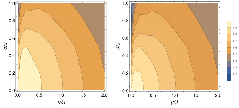
Figure 6: Contour-plots of the transfer efficiency $\bar{p}_{\rm sink}^{M}(t)$ (10) at time $Jt=100$ as a function of the ratio $\gamma/J$ and of $\sigma/J$ for (a) the isotropic ring and (b) the dimerized ring.

An intuitive explanation of can be given as follows: disorder introduces random phases between adjacent sites that would be responsible of the localization of the excitation in the neighbourhood of its initial condition, while dephasing tends to “wash-away” the ensuing interference patterns. In figure 7 we show a comparison between the sink population in the presence of the sole disorder ($\sigma/J=0.5$) and in the presence of the same amount of disorder and dephasing ($\gamma/J=0.1$). The selected parametrization is suggested by an inspection of figure 6.

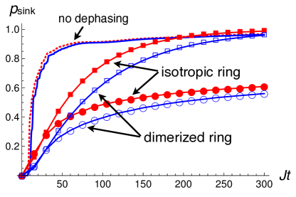
Figure 7: The (average) sink population as a function of $Jt$. Circles: sink population in the presence of disorder with $\sigma/J=0.5$. Squares: sink population in the presence of the same amount of disorder and dephasing for $\gamma/J=0.1$ Filled red markers refer to the isotropic case, empty blue markers to the dimerized configuration. Dashed red line and solid blue line represent the sink population in the absence of dephasing and disorder for the isotropic and dimerized ring respectively and are reported for comparison purposes.

Dephasing, therefore, enhances transport in the presence of disorder already at a time-scale comparable to the propagation time of the excitation from its initial location to the opposite site $j=17$. The suppression of the localization of the excitation is made more evident by the faster increase of the sink population. Even in the presence of disorder, moreover, dephasing still allows, in the long-time limit, to increase the sink population beyond the value reached in the absence of both dephasing and disorder.

5 Conclusion and Outlook

Dephasing assisted transport is an example of how an interplay between the coherent and incoherent part of system dynamics can lead to an improvement of the energy transfer between different points of graph. In this work we have investigated DAT over a circular graph with isotropic and alternate couplings between nearest-neighbour sites in the presence of disorder and dephasing. Our analysis confirmed the existence of regimes where DAT occurs.

We showed that dimerization does not provide an advantage for the energy transfer process over disordered systems affected by decoherence. While the model of the system and of the effects induced by the system-enviromnent interaction we adopted is highly simplified and might not capture some key feature of the light-harvesting complexes, our results hint that the functional advantage of the dimerized structure of LH1/2 complexes cannot be captured by a quantum-walk perspective.

Future work will address the inclusion of losses, dissipation and thermalization, as to understand whether the time-scales on which DAT occurs are compatible with the exciton loss and relaxation rates of the system. More refined models [32, 33, 34], where the effective Markovian dynamics is replaced by scattering processes on the lattice hosting the TLSs will be considered as well.

References

- [1] A. Childs, E. Farhi and S. Gutmann, Quantum Information Processing 1 (2002) 35
- [2] A. M. Childs et al., Exponential algorithmic speedup by a quantum walk, in Proc. 35th ACM Symp. STOC 2003, STOC ’03 (ACM, New York, NY, USA, 2003)
- [3] M. Christandl et al., Phys. Rev. A 71 (2005) 032312
- [4] D. Tamascelli et al., Sci. Rep. 6 (2016) 26054
- [5] S. Bose, Cont. Phys. 48 (2007) 13
- [6] O. Mülken and A. Blumen, Phys. Rep. 502 (2011) 37
- [7] G. S. Engel et al., Nature 446 (2007) 782
- [8] H. Lee, Y.-C. Cheng and G. R. Fleming, Science 316 (2007) 1462
- [9] G. Panitchayangkoon et al., PNAS 107 (2010) 12766
- [10] R. J. Sension, Nature 446 (2007) 740
- [11] A. Olaya-Castro, et al., Phys. Rev. B 78 (2008) 085115
- [12] M. Plenio and S. Huelga, New J. Phys. 10 (2008) 113019
- [13] F. Caruso et al., J. Chem. Phys. 131 (2009) 105106
- [14] M. Sarovan et al., Nature Physics 6 (2010) 462
- [15] C. Smyth, F. Fassioli and G. Scholes, Phil. Trans. R. Soc. A 370 (2012) 3728
- [16] S. Sangwoo, P. Rebentrost, S. Valleau and A. Aspuru-Guzik, Biophys. J. 102 (2012) 649
- [17] G. Scholes, G. Fleming, A. Olaya-Castro and R. van Grondelle, Nature Chemistry 3 (2011) 763
- [18] P. Rebentrost et al., New J. Phys. 11 (2008) 033003
- [19] M. Mohseni et al., J. Chem. Phys. 129 (2008) 174106
- [20] L. D. Contreras-Pulido et al., New J. Phys. 16 (2014) 113061
- [21] S. Niwa et al., Nature 508 (2014) 228
- [22] F. Caycedo-Soler et al., eprint arXiv:1504.05470v2 [physics.bio-ph] (2015)
- [23] Y. Zhao, M. F. Ng and G. Chen, Phys. Rev. E 69 (2014) 032902
- [24] F. Caycedo-Soler et al., eprint arXiv:1107.0191v1 [cond-mat.soft] (2011)
- [25] W. M. Itano, J. Phys.: Conf. Series 196 (2009) 012018
- [26] G. D. Scholes and G. R. Fleming, The Journal of Physical Chemistry B 104 (2000) 1854
- [27] K. Timpmann et al., Chem. Phys. Lett. 414 (2005) 359
- [28] M. K. Sener, J. D. Olsen, C. N. Hunter and K. Schulten, PNAS 104 (2007) 15723
- [29] E. Abrahams et al., Phys. Rev. Lett. 42 (1979) 673
- [30] F. Domínguez-Adame and V. A. Malyshev, Am. J. Phys 72 (2004) 226
- [31] D. de Falco and D. Tamascelli, J. Phys. A: Math. Theor. 46 (2013) 225301
- [32] M. Bednarz, V. A. Malyshev and J. Knoester, J. Chem. Phys. 128 (2004) 3827
- [33] D. J. Heijs, V. A. Malyshev and J. Knoester, J. Chem. Phys. 123 (2005) 144507
- [34] D. J. Heijs, V. A. Malyshev and J. Knoester, J. Lum. (2006) 271
- [35] A. W. Chin et al., New J. Phys. 12 (2010) 065002