Morse index for figure-eight choreographies of the planar equal mass three-body problem

Abstract

We report on numerical calculations of Morse index for figure-eight choreographic solutions to a system of three identical bodies in a plane interacting through homogeneous potential, $-1/r^{a}$, or through Lennard-Jones-type (LJ) potential, $1/r^{12}-1/r^{6}$, where $r$ is a distance between the bodies. The Morse index is a number of independent variational functions giving negative second variation $S^{(2)}$ of action functional $S$. We calculated three kinds of Morse indices, $N$, $N_{c}$ and $N_{e}$, in the domain of the periodic, the choreographic and the figure-eight choreographic function, respectively. For homogeneous system, we obtain $N=4$ for $0\leq a<a_{0}$, $N=2$ for $a_{0}<a<a_{1}$, $N=0$ for $a_{1}<a$, and $N_{c}=N_{e}=0$ for $0\leq a$, where $a_{0}=0.9966$ and $a_{1}=1.3424$. For $a=1$, we show a strong relationship between the figure-eight choreography and the periodic solution found by Simó through the $S^{(2)}$. For LJ system, we calculated the index for the solution tending to the figure-eight solution of $a=6$ homogeneous system for the period $T\to\infty$. We obtain $N$, $N_{c}$ and $N_{e}$ as monotonically increasing functions of the gradual change in $T$ from $T\to\infty$, which start with $N=N_{c}=N_{e}=0$, jump at the smallest $T$ by $1$, and reach $N=12$, $N_{c}=4$, and $N_{e}=1$ for $T\to\infty$ in the other branch.

1 Introduction

Choreographic motion of $N$ bodies is a periodic motion on a closed orbit, $N$ identical bodies chase each other on the orbit with equal time-spacing. Moore [1] found a remarkable figure-eight three-body choreographic solution under homogeneous potential $-1/r^{a}$ by numerical calculations, where $r$ is a distance between bodies. Chenciner and Montgomery [2] gave a mathematical proof of its existence for $a=1$ by variational method. The detailed initial conditions for three bodies are found in [2, 10].

Sbano [3], Sbano and Southall [4], and Fukuda et al [5], after that, studied $N$-body choreographic solutions under an inhomogeneous potential

$$u^{LJ}(r)=\frac{1}{r^{12}}-\frac{1}{r^{6}},$$ (1)

a model potential between atoms called Lennard-Jones-type (hereafter LJ) potential. Sbano and Southall [4] proved that there exist at least two $N$-body choreographic solutions for sufficiently large period $T$, and there exists no solution for small period $T$. Then we confirmed their theorem numerically and unexpectedly found a multitude of figure-eight choreographic solutions under LJ potential (1) [5].

Recently, Shibayama [6] calculated Morse index numerically for the figure-eight and for super-eight choreography to consider the variational proof of their existence. Here Morse index is a number of independent variational functions giving negative second variation of action functional.

There are several researches on Morse indices for periodic solution of three body problem. Barutello et al [7] calculated Morse index mathematically for the Lagrangian circular orbit, and Hu and Sun [8, 9] for elliptic Lagrangian solutions, to discuss the linear stability.

In this paper, we calculate Morse indices numerically for the figure-eight choreographies to a system of three identical bodies interacting through a homogeneous potential or through LJ potential (1). We expect that accurate numerical calculations of Morse index will reveal their structures and relations via the geometry of their action manifolds. In section 2, we define Morse index and present corresponding eigenvalue problem and our method of its numerical calculation. In section 3, Morse index for the system interacting through homogeneous potential with various $a\geq 0$ are calculated. For $a=1$ we point out strong relationship between the figure-eight choreography and periodic solution close to it found by Simó [10] through the second variation of action functional. In section 4, we calculate the Morse index for a solution we found [5] in the system interacting through LJ potential (1), tending toward the figure-eight choreography in the homogeneous system with $a=6$ for $T\to\infty$. We discuss the Euler characteristic of their action manifold. Further the correspondence of the results between LJ and homogeneous system is investigated. Section 5 is a summary and discussions. Our numerical results in this paper were calculated by Mathematica 11.1 in its default precision, unless otherwise stated.

2 Numerical calculation of Morse index

2.1 Eigenvalue problem for Morse index

For a system of three identical bodies in classical mechanics, we consider periodic solutions to equations of motion,

$$\frac{d}{dt}\frac{\partial L}{\partial\dot{q}_{i}}=\frac{\partial L}{\partial q_{i}},\;i=1,2,\ldots,6,$$ (2)

where dot represents a differentiation in $t$. $L$ is the Lagrangian with the potential energy $U(q)$

$$L(q,\dot{q})=\sum_{i=1}^{6}\frac{\dot{q}_{i}^{2}}{2}-U(q),$$ (3)

and

$$q(t)=(q_{1}(t),q_{2}(t),\ldots,q_{6}(t))^{*}$$ (4)

a six component vector composed of position vectors

$$\bi{r}_{b}(t)=(x_{b}(t),y_{b}(t))^{*}=(q_{2b-1}(t),q_{2b}(t))^{*}$$ (5)

for body $b=1,2,3$ moving in a plane, where ^∗ represents transpose.

For a periodic solution $q(t+T)=q(t)$ with period $T$, we calculate the second variation of the action

$$S(q)=\int_{0}^{T}L(q,\dot{q})dt.$$ (6)

The $k$’th variation $S^{(k)}$ of the action $S(q)$ is defined as the $k$’th coefficients in

$$S(q+h\delta q)=S^{(0)}+hS^{(1)}+\frac{h^{2}}{2!}S^{(2)}+\cdots,$$ (7)

thus

$$S^{(k)}=\int_{0}^{T}dt\left(\sum_{i}(\delta q_{i}\frac{\partial}{\partial q_{i}}+\dot{\delta q}_{i}\frac{\partial}{\partial\dot{q}_{i}})\right)^{k}L,$$ (8)

where $h$ is a real number and $\delta q$ is a variation function with period $T$, $\delta q(t+T)=\delta q(t)$.

By partial integration, the second variation is written as

$$S^{(2)}=(\delta q,\hat{H}\delta q)$$ (9)

by $6\times 6$ matrix operator $\hat{H}$,

$$\hat{H}_{ij}=-\delta_{ij}\frac{d^{2}}{dt^{2}}-U_{ij}(t),$$ (10)

with

$$U_{ij}(t)=\frac{\partial^{2}U}{\partial q_{i}\partial q_{j}}.$$ (11)

The inner product $(f,g)$ is defined as

$$(f,g)=\int_{0}^{T}dtf^{*}g$$ (12)

and $\delta_{ij}$ the Kronecker delta. Considering eigenvalue $\lambda$ and eigenfunction $\psi$ of the operator $\hat{H}$,

$$\hat{H}\psi=\lambda\psi,$$ (13)

the second variation for $\delta q=\psi$ is given by

$$S^{(2)}=\lambda.$$ (14)

Then the Morse index is the number of negative eigenvalues of (13). Here the eigenfunction $\psi$ is assumed to be normalized as

$$(\psi,\psi)=1.$$ (15)

2.2 Figure-eight choreographic, choreographic and non-choreographic eigenfunction

We consider the eigenvalue problem (13) for a figure-eight choreography $q$. A function $f$ is called choreography or choreographic if $f$ satisfies

$$\hat{C}f=f$$ (16)

where the linear operator $\hat{C}$ is defined by

$$\hat{C}f_{i}(t)=f_{i+2}(t-\frac{T}{3}).$$ (17)

A figure-eight choreography is a choreography with its orbit symmetric in $x$- and $y$-axis. Here in (17) and hereafter the subscript of six component vector is assumed to be in the range between 1 and 6 with translation by 6.

Then the eigenfunction $\psi$ with period $T$ of (13) is classified into the following three types: 1) Choreographic eigenfunction if $\psi$ is choreographic, which is possible since $\hat{C}$ and $\hat{H}$ commute. 2) Figure-eight choreographic eigenfunction if $q+h\psi$ is figure-eight choreographic. 3) Non-choreographic eigenfunction is a orthogonal complement of choreographic eigenfunction.

Accordingly, we obtain three kind of Morse index at the figure-eight choreography $q$ in different domain from the common eigenvalue problem (13) for periodic $\psi$: Morse index in the domain of the periodic function, the choreographic function, and the figure-eight choreographic function. In the following we denote these three Morse indices in the different domains as $N$, $N_{c}$ and $N_{e}$, respectively.

Note that variational functions representing translation in $x$- and $y$-direction, rotation, and translation in time, keep the action integral $S(q)$ constant, and their derivatives are the eigenfunctions of zero eigenvalues. Therefore the zero eigenvalues of (13) are quadruply degenerated and their eigenfunctions correspond to the conservation law of linear and angular momentum, and energy, respectively.

Further the equation (13) has trivial solutions

$$\lambda=k^{2}\omega^{2},\;k=1,2,3,\ldots,$$ (18)

$$\psi(t)=(x(t),y(t),x(t),y(t),x(t),y(t))^{*}$$ (19)

with $x(t)=\sin{k\omega t}$ or $\cos{k\omega t}$, and $y(t)=\sin{k\omega t}$ or $\cos{k\omega t}$, where $\omega=2\pi/T$. Since $U(q)$ is functions of $|\bi{r}_{b}-\bi{r}_{c}|$ unaffected by the variation $\delta q(t)=\psi(t)$ in (19), $\delta^{2}U=0$, $\sum_{j}U_{ij}\psi_{j}=0$ and $\hat{H}\psi=-d^{2}\psi/dt^{2}$. Thus the solutions (18) and (19) are derived. We call this quadruply degenerated eigenfunctions trivial [11].

2.3 Fourier series expansion

Following Shibayama [6], we solve the eigenvalue problem (13) by expanding the $\psi$ in the Fourier series

$$\psi_{i}(t)=\sum_{k=0}^{M-1}v_{k}^{(i)}\phi_{k}(t)$$ (20)

where

$$\phi_{k}(t)=\left\{\begin{array}[]{l l}\displaystyle\sqrt{\frac{2}{T}}\sin(\frac{k+1}{2}\omega t)&k=1,3,5,\ldots\\ \displaystyle\sqrt{\frac{2}{T(1+\delta_{k0})}}\cos(\frac{k}{2}\omega t)&k=0,2,4,\ldots\\ \end{array}\right.$$ (21)

are the normalized basis as

$$\int_{0}^{T}\phi_{k}\phi_{l}dt=\delta_{kl}.$$ (22)

Thus (13) becomes the eigenvalue problem

$$Hv=\lambda v$$ (23)

for $6M\times 6M$ real symmetric matrix $H$

$$H_{6k+i,6l+j}=\int_{0}^{T}dt\phi_{k}\hat{H}_{ij}\phi_{l}=-u_{6k+i,6l+j}+\omega^{2}\lfloor\frac{k+1}{2}\rfloor^{2}\delta_{ij}\delta_{kl},$$ (24)

where

$$u_{6k+i,6l+j}=\int_{0}^{T}dt\phi_{k}U_{ij}(t)\phi_{l}$$ (25)

and $\lfloor.\rfloor$ is the floor function. The vector $v$ is a column vector of $6M$ components, $v_{6k+i}=v_{k}^{(i)},$ with

$$v^{*}v=1$$ (26)

by the normalization condition (15).

The matrix elements (25) are calculated from about $42M$ integrals

$$u_{ij}(k)=u_{ij}^{(+)}(k)+\imath u_{ij}^{(-)}(k)=\frac{2}{T}\int_{0}^{T}dt\exp(\imath k\omega t)U_{ij}(t)$$ (27)

as

$$u_{6k+i,6l+j}=\left\{\begin{array}[]{l l}\displaystyle\frac{p^{l}}{2}u_{ij}^{(p)}(k^{\prime}-l^{\prime})+\frac{(-1)^{kl}}{2}u_{ij}^{(p)}(k^{\prime}+l^{\prime}),&(k>0,l>0)\\ \displaystyle\frac{1}{\sqrt{1+\delta_{k0}}\sqrt{1+\delta_{l0}}}u_{ij}^{(p)}(k^{\prime}+l^{\prime}),&(\mbox{otherwise})\end{array}\right.$$ (28)

where

$$p=(-1)^{k+l},\;k^{\prime}=\lfloor\frac{k+1}{2}\rfloor,\;l^{\prime}=\lfloor\frac{l+1}{2}\rfloor,$$ (29)

and $\imath=\sqrt{-1}$. Though the upper first term in (28) looks non symmetric in $k$ and $l$ at a glance, it is symmetric as defined by (25) since $p^{l}=-p^{k}$ for $p=-1$.

We evaluate the integral (27) with periodic integrand efficiently by trapezoidal formula of numerical integration with $n$ points and it is done by fast Fourier transform quickly.

3 Homogeneous potential

For the system interacting through the homogeneous potential

$$U(q)=-\sum_{b>c}\frac{1}{r_{bc}^{a}}$$ (30)

where $r_{bc}=|\bi{r}_{b}-\bi{r}_{c}|$, we calculated the matrix elements (25) for $0\leq a\leq 7$. The number of points for the trapezoidal formula is $n=3\times 2^{11}$ and terms for the Fourier series (20) $M=161$. Here $n$ is multiple of 3 to make the set of points for the numerical integration closed in the translation in $t$ by $T/3$. The estimated error in numerical integration is less than $10^{-9}$ and lower twenty eigenvalues are obtained in 6 digits.

3.1 Morse index and eigenfunctions for $a=1$

In figure 1, for $a=1$, twenty eigenvalues and eigenfunctions for the figure-eight choreography $q$ with size $x_{\max}=\max{x_{b}(t)}=2$ and period $T=T_{1}=15.919135$ are shown in the ascending order from the minimum eigenvalue. In figure 1, the eigenfunction $\psi$ itself is not shown but the variated orbit $\bi{r}_{b}+h\delta\bi{r}_{b}$, $b=1,2,3$ with $h=1.5$ is displayed by light, medium and dark gray curves, respectively, together with the orbit $\bi{r}_{1}$ by dashed curve, where $\delta\bi{r}_{b}$ is the body $b$ component of $\psi$ defined by

$$\delta\bi{r}_{b}=(\psi_{2b-1},\psi_{2b})^{*}.$$ (31)

The variated orbits are more physical and convenient for understanding the characteristics of eigenfunctions though they include a parameter $h$ than eigenfunction itself.

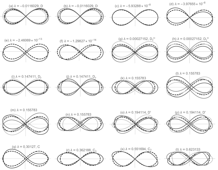
Figure 1: The eigenvalues, orbits $\bi{r}_{1}$ (dashed curve) for $a=1$, $x_{\max}=2$, $T=T_{1}=15.919135$, $S=33.225363$ and the variated orbits $\bi{r}_{b}+h\delta\bi{r}_{b}$, $b=1,2,3$ ( light, medium and dark gray curves, respectively), $h=1.5$. Symbols at the end of the labels are those of eigenfunctions explained in table 1.

The four eigenvalues in figure 1 (c) to (f) are close to zero and from the variated orbits we can see that they represent the translation in time, rotation, and translation in $x$- and $y$-direction, respectively. Thus they are four zero eigenvalues originated in the conservation law. The quadruply degenerated eigenvalues $\lambda=0.155783=\omega^{2}$ in figure 1 (k) to (n) are trivial. Also the $\lambda=0.623133=4\omega^{2}$ in figure 1 (t) is one of the quadruply degenerated trivial eigenvalues with $k=2$.

The eigenvalues in figure 1 (q), (r) and (s) are non-degenerated. We show if an eigenvalue is non-degenerated like that its eigenfunction is choreographic, thus they are choreographic. Suppose $\lambda$ is non-degenerated eigenvalue and $\psi$ its eigenfunction. Since $\hat{H}$ and $\hat{C}$ commute, $\hat{C}\psi$ is also the eigenfunction of $\lambda$, thus $\hat{C}\psi=c\psi$ where $c$ is a real coefficient. Then $\hat{C}^{3}=1$ leads $c^{3}=1$ and $\hat{C}\psi=\psi$ which means $\psi$ is choreographic.

For choreographic eigenfunction $\psi$ the three variated orbits overlap and differ only in time shift,

$$\bi{r}_{c}(t)+h\delta\bi{r}_{c}(t)=\bi{r}_{b}(t^{\prime})+h\delta\bi{r}_{b}(t^{\prime}),\;t^{\prime}=t+(c-b)T/3,$$

by $\hat{C}q=q$ and $\hat{C}\psi=\psi$ with (17). Thus full curves in figure 1 (q), (r) and (s) overlap and appear as one. Further, among the three choreographic eigenfunctions only the variated orbit (r) is symmetric in both $x$- and $y$-axis, thus it is the only figure-eight choreographic eigenfunction.

The pair of successive eigenvalues (a) and (b), (g) and (h), (i) and (j), and (o) and (p) in figure 1 are doubly degenerated and their variated orbits are splited into distinct full curves. We show that any linear combination of such degenerated eigenfunctions can not be choreographic, thus they are non-choreographic. Suppose $\psi^{(s)}$ and $\psi^{(s+1)}$ are the exactly doubly degenerated orthonormal eigenfunctions having distinct full curves. Thus $\hat{C}\psi^{(s)}\neq\psi^{(s)}$ and $\hat{C}\psi^{(s+1)}\neq\psi^{(s+1)}$ since $\hat{C}q=q$. Since the operator $\hat{C}$ commutes with $\hat{H}$, conserves inner product as $(\hat{C}f,\hat{C}g)=(f,g)$, and $\hat{C}^{3}=1$, the $\hat{C}$ is represented as $\theta_{c}=\pm 2\pi/3$ rotation

$$R(\theta_{c})=\left(\begin{array}[]{r r}\cos\theta_{c}&-\sin\theta_{c}\\ \sin\theta_{c}&\cos\theta_{c}\end{array}\right)$$ (32)

in the base functions $\psi^{(s)}$ and $\psi^{(s+1)}$. Here the sign of $\theta_{c}$ is fixed by the phase of the base functions. Thus for any linear combination $\psi=h_{1}\psi^{(s)}+h_{2}\psi^{(s+1)}$, $\hat{C}\psi=\psi$ represented by $R(\theta_{c})(h_{1},h_{2})^{*}=(h_{1},h_{2})^{*}$ leads $(h_{1},h_{2})=0$ which means $\psi$ can not be choreographic.

Now we can count three kind of Morse index for $a=1$ in the different domains from figure 1. Since there are two negative eigenvalues, (a) and (b) in figure 1, Morse index $N$ is counted as 2. They are doubly degenerated and have distinct full curves, therefore $N_{c}$ for choreographic and $N_{e}$ for figure-eight choreographic domain are both counted as 0.

3.2 Morse index for $a\geq 0$

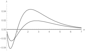
Figure 2: The lowest eight eigenvalues $\lambda$’s for eigenvalue problem (23) for homogeneous potential with $0<a\leq 7$.

In figure 2, for $0<a\leq 7$, the lowest eight eigenvalues for the figure-eight choreography with the same size $x_{\max}=2$ are plotted as functions of $a$. Two curves are doubly degenerated and there are four lines on the $x$-axis which are four zero eigenvalues.

The Morse indices for $0\leq a$ are

$$N=\left\{\begin{array}[]{l l}4&(0\leq a<a_{0}),\\ 2&(a_{0}<a<a_{1}),\\ 0&(a_{1}<a),\end{array}\right.$$ (33)

and

$$N_{c}=N_{e}=0\;(0\leq a),$$ (34)

where

$$a_{0}=0.9966,\;a_{1}=1.3424.$$ (35)

Here $a=0$ is calculated by the log potential

$$U(q)=\sum_{b>c}\log r_{bc}$$ (36)

and $a>7$ are extrapolated.

The characteristics of the variated orbits for $a\neq 1$ are almost similar for $a=1$ shown in figure 1 though the order of the eigenvalues may be changed. For example, at $a=1.5$, the first four eigenvalues are zero and the fifth and the sixth variated orbits are similar to the first and the second in figure 1, as read in figure 2. We present precise table for characteristics of the variated orbits in section 4.1.

3.3 Simó’s H orbits

The three orbits, H1, H2 and H3, found by Simó [10] are very close to the variated orbits by non-choreographic eigenfunctions for $a=1$.

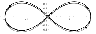
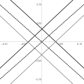
(a)                                (b)

Figure 3: (a) Simó’s H3 orbit [10] rotated by 0.277217 rad scaled to unit mass $m=1$ and $T=T_{1}=15.919135$. (b) The same figure around the origin.

In figure 3, the H3 orbit rotated and scaled to $T=T_{1}$, $q^{H3}(t)$, are shown. It consists of three slightly different eight shaped orbits, one of them is passing through the origin as shown in figure 3 (b). The set of orbits is symmetric in both $x$ and $y$ inversion where the two orbits are exchanged in $y$ inversion. The orbits H1 and H2 are the same orbit as H3 by rotation, translation in time and permutation of bodies.

The variated orbit

$$q(t)+h\psi^{(\Theta)}(t)$$ (37)

by doubly degenerated $s$’th and $(s+1)$’th eigenfunctions $\psi^{(s)}$ and $\psi^{(s+1)}$,

$$\psi^{(\Theta)}(t)=\cos\Theta\psi^{(s)}(t)+\sin\Theta\psi^{(s+1)}(t),$$ (38)

is very close to $q^{H3}$ at $s=7$, $h=h_{H}=0.28375$ and some $\Theta=\Theta_{H}$. Actually the squared difference between $q^{H3}$ and $q+h_{H}\psi^{(\Theta_{H})}$ averaged in $t$ is less than $10^{-7}$. The variated orbits for $\psi^{(7)}$ and $\psi^{(8)}$ are shown in figure 1 (g) and (h). They are symmetric in $y$-axis but not in $x$-axis. The linear combination (38) with $\Theta=\Theta_{H}$ makes it symmetric in $x$-axis.

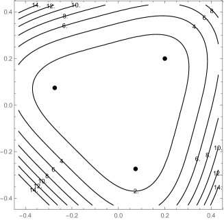
Figure 4: Contour plot for action $S(q+h\psi^{(\Theta)})$ where horizontal and vertical axis are $h\cos\Theta$ and $h\sin\Theta$, respectively. Contours are labeled by $(S(q+h\psi^{(\Theta)})-S(q))\times 10^{5}$.

In figure 4, the contour plot of action $S(q+h\psi^{(\Theta)})$ is shown where horizontal and vertical axis are $h\cos\Theta$ and $h\sin\Theta$, respectively. The contours in figure 4 show the three fold symmetry since $\hat{C}$ is represented by $\theta_{c}=\pm 2\pi/3$ rotation (32) and conserves $S$ as $S(\hat{C}f)=S(f)$.

One of the three black points in figure 4 is the point $(h_{H},\Theta_{H})$ closest to the critical point $q^{H3}$ of action functional, and the other two $(h_{H},\Theta_{H}\pm 2\pi/3)$ its cyclic permutations of bodies with time shift, $\hat{C}q^{H3}$ and $\hat{C}^{2}q^{H3}$.

The action $S(q^{H3})=33.22536589$ at $q^{H3}$ is slightly higher than $S(q)=33.22536229$ at $q$, thus the critical point $q^{H3}$ will be local maximum towards $q$. Here $S(q^{H3})$ and $S(q)$ are obtained in multiple precision calculation by the initial conditions in [10], and no shallow local maximum is found numerically in the plane around the black points in figure 4. Nevertheless $h_{H}$ is about $0.282$ estimated by

$$h=\sqrt{\frac{6|S(q^{\prime})-S(q)|}{|\lambda|}}$$ (39)

with $q^{\prime}=q^{H3}$, which assumes critical at $h$. The estimation (39) is derived by equating $S(q^{\prime})$ and the $S(q+h\psi)$ truncated at $h^{3}$ term in (7) regarding $S^{(3)}$ as a parameter, $S(q)+h^{2}\lambda/2+h^{3}S^{(3)}/3!,$ with the critical condition at $h$, $h\lambda+h^{2}S^{(3)}/2=0$.

Note that Simó’s $q^{H3}$ approximately satisfies the relation [10]

$$q_{i}(t)\simeq\frac{1}{3}\sum_{k=0}^{2}q_{i+2k}^{H3}(t-\frac{kT}{3})$$ (40)

or

$$q\simeq\frac{1+\hat{C}+\hat{C}^{2}}{3}q^{H3}$$ (41)

since $q+h_{H}\psi^{(\Theta_{H})}$ at $s=7$ is very close to $q^{H3}$ and

$$(1+\hat{C}+\hat{C}^{2})\psi^{(\Theta)}=0$$ (42)

by equation (32).

4 Lennard-Jones-type potential

For the system interacting through the LJ potential

$$U(q)=\sum_{b>c}u^{LJ}(r_{bc}),$$ (43)

we calculated the Morse index of the solution $\alpha$ [5]. The solution $\alpha$ is the figure-eight choreographic solution asymptotically tending to that under homogeneous potential with $a=6$ at $T\to\infty$. In figure 5, $S(q)$ for the solution $\alpha$ is shown against $T$. There are two branches of $S(q)$ branched at $T=T_{\min}=14.4793$, the minimum period $T$ of solution $\alpha$, as shown in figure 5. We denote the branch with higher action value $S$ as the $\alpha_{+}$ and lower the $\alpha_{-}$.

The shape of the orbit gradually changes from the figure-eight for $\alpha_{-}$ shown in figure 5 (a), via the branch point $T=T_{\min}$ in figure 5 (b), to the gourd shape for $\alpha_{+}$ shown in figure 5 (c). Though the $S(q)$ shows cusp like shape at $T=T_{\min}$, $q$ changes smoothly there. The characteristics of the eight-shaped choreographic orbits of $\alpha_{-}$ for $T\to\infty$ are very close to those for the $a=6$ homogeneous potential since the particles have large relative distances and the short-range repulsive part of the LJ potential is less important [5].

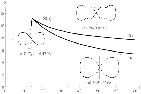
Figure 5: Action $S(q)$ for the figure-eight solution $\alpha$ against $T$ and the orbit $q$ under LJ potential. (a) Figure-eight orbit with $x_{\max}=2$ ($T=61.7495$) in $\alpha_{-}$ branch. (b) Figure-eight orbit at $T=T_{\min}=14.4793$, branch point. (c) Gourd shaped orbit with $x_{\max}=2$ ($T=49.0118$) in $\alpha_{+}$ branch. The three orbit, (a)–(c) are drawn in relatively correct size.

The numerical calculations are done with $3\times 2^{11}\leq n\leq 3\times 2^{14}$ and $321\leq M\leq 10241$ for $T_{\min}\leq T<100$, and lower twenty eigenvalues are obtained at least 5 digits. For the solution $\alpha_{+}$ the gourd shape is sharper for larger $T$ and sharp spikes appear in the matrix elements $U_{ij}(t)$ as shown in figure 6, which make the numerical integration for the $\alpha_{+}$ for $T>100$ difficult.

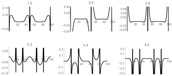
Figure 6: Independent elements of $U_{ij}(t)$ for solution $\alpha_{+}$ at $T=98.0332$ ($x_{\max}=2.4$). Each graph is titled by $i,j$.

We obtain for $\alpha_{-}$

$$N(\alpha_{-})=\left\{\begin{array}[]{l l}5&(14.4793\leq T<14.5952),\\ 4&(14.5952<T<14.8358),\\ 2&(14.8358<T<14.8611),\\ 0&(14.8611<T),\\ \end{array}\right.$$ (44)

$$N_{c}(\alpha_{-})=\left\{\begin{array}[]{l l}1&(14.4793\leq T<14.5952),\\ 0&(14.5952<T),\\ \end{array}\right.$$ (45)

$$N_{e}(\alpha_{-})=0\;(14.4793\leq T),$$ (46)

and for $\alpha_{+}$

$$N(\alpha_{+})=\left\{\begin{array}[]{l l}6&(14.4793\leq T<16.1110),\\ 8&(16.1110<T<16.8779),\\ 10&(16.8687<T<17.1317),\\ 11&(17.1317<T<18.6154),\\ 12&(18.6154<T),\end{array}\right.$$ (47)

$$N_{c}(\alpha_{+})=\left\{\begin{array}[]{l l}2&(14.4793\leq T<17.1317),\\ 3&(17.1317<T<18.6154),\\ 4&(18.6154<T),\end{array}\right.$$ (48)

$$N_{e}(\alpha_{+})=1\;(14.4793<T).$$ (49)

For $T>100$ all indices are extrapolated.

In figure 7, the indices $N$, $N_{c}$ and $N_{e}$ are plotted against $T$ for $\alpha_{+}$ and $\alpha_{-}$ together.

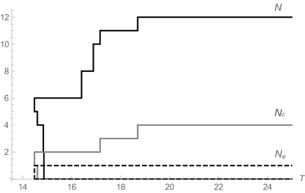
Figure 7: $N$, $N_{c}$ and $N_{e}$ for the solution $\alpha$.

All the $N$, $N_{c}$ and $N_{e}$, increase from $0$ monotonically to $12$, $4$ and $1$, respectively, starting from infinitely large $T$ in $\alpha_{-}$. They all jump by one at $T=T_{\min}$.

4.1 Correlation of eigenfunctions

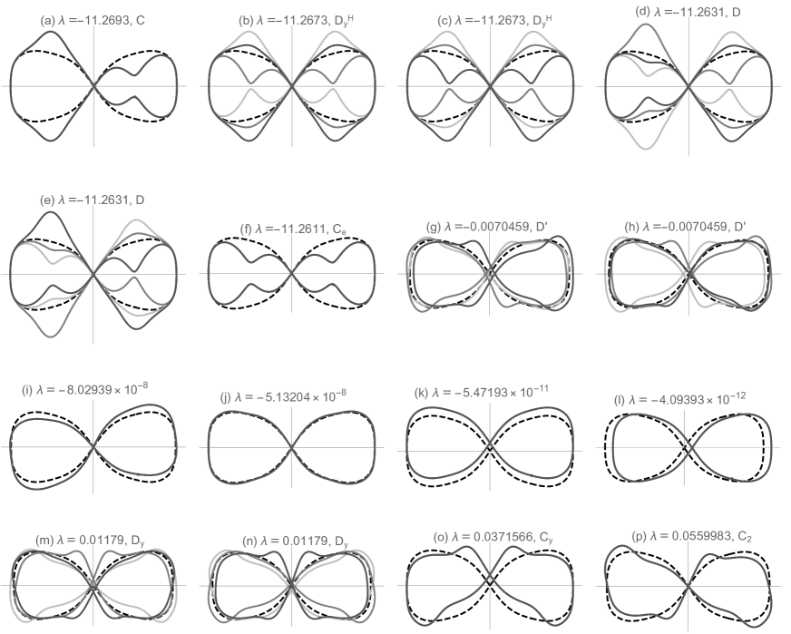
Figure 8: The eigenvalues, orbits $\bi{r}_{1}$ (dashed curve) for solution $\alpha_{+}$ under LJ potential, $x_{\max}=1.44$, $T=16.4019$, $S=10.8136$, and the variated orbits $\bi{r}_{b}+h\delta\bi{r}_{b}$, $b=1,2,3$ (light, medium and dark gray curves, respectively) with $h=1$. Symbols at the end of the labels are those of eigenfunctions explained in table 1.

In figure 8, lower sixteen eigenvalues and eigenfunctions for the solution $\alpha_{+}$ at $T=16.4019$ are shown in the same style as figure 1. Instead of exhibiting a huge number of similar lists as figure 8 for different $T$, we make figure 8 representative and show how they change. When the period $T$ changes, either in the $\alpha_{+}$ or $\alpha_{-}$ branch, the different eigenfunctions change continuously with $T$.

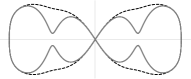
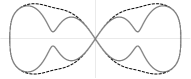
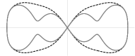
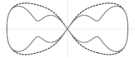
(a) $T=19.0588$       (b) $T=18.3370$       (c) $T=17.0085$       (d) $T=16.4019$

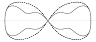
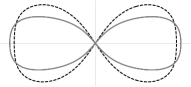
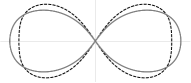
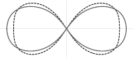
(e) $T=15.3047$       (f) $T=14.4869$       (g) $T=14.6763$       (h) $T=14.8420$      
                              
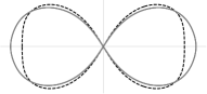
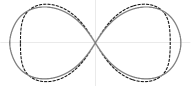
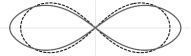
(i) $T=61.7495$           (j) $a=6$                   (k) $a=1$

Figure 9: The eigenvalues, orbits $\bi{r}_{1}$ (dashed curve) and the variated orbits $\bi{r}_{b}+h\delta\bi{r}_{b}$, $b=1,2,3$ (light, medium and dark gray curves, respectively) correlated to those shown in figure 8 (f) or to eigenfunction $C_{e}$ defined in table 1, with $h=3$ for (i) and (j), $h=1.5$ for (k), and $h=1$ for the others.

For example, changes of figure 8 (f) are shown in figure 9. Starting from the figure 9 (d) which is figure 8 (f), figures 9 (a)–(e) show continuous changes in the $\alpha_{+}$ branch and figures 9 (f)–(i) in the $\alpha_{-}$ branch.

Since the $\alpha_{-}$ solution for $T\to\infty$ tends to the solution for the $a=6$ homogeneous system, their eigenfunctions and the variated orbits also do so. In the case of figure 9, (i) and (j) are very close since they are the variated orbits for the $\alpha_{-}$ for large $T$ and the $a=6$ homogeneous system, respectively.

We call the eigenfunction obtained by changing continuous parameter, $T$ or $a$, correlated. We also call two eigenfunctions, one for $\alpha$ solution with $T$ and the other homogeneous system with $a$, if they are identical at $T\to\infty$ in the $\alpha_{-}$ branch and at $a=6$, correlated. In figure 9, the eigenfunctions of all variated orbits, (a)–(k), are correlated since (i) and (j) are correlated.

In table 1 eigenfunctions correlated to those shown in figure 8, except for the trivial eigenfunctions, are tabulated. Each row shows the eigenfunctions by symbols in ascending order of eigenvalues for the solution shown in the left three columns. The symbol $C$ represents non-degenerated choreographic eigenfunction, $D$ doubly degenerated non-choreographic eigenfunctions and $0$ quadruply degenerated eigenfunctions of the zero eigenvalue.

The subscript in the symbol indicates the symmetry of the variated orbits. $y$ indicates they are symmetric in $y$ axis, $e$ in both $x$ and $y$ axis, and 2 in 2 fold rotation at origin. Prime are used to distinguish different eigenfunctions with the same characters. The superscript $H$ identifies the eigenfunction corresponding to the Simó’s H obits discussed in section 3.3 for $a=1$, (g) and (h) in figure 1.

These symbols defined here are added at the end of each label in figure 1 and 8 except for 0’s. The variated orbits shown in figure 9 are those with the eigenfunction $C_{e}$.

Table 1: The correlation table for eigenfunctions. Each row shows the type of eigenfunctions in ascending order of the eigenvalue. $C$; a choreographic eigenfunction. $D$; doubly degenerated non-choreographic eigenfunctions. $0$; quadruply degenerated eigenfunctions of zero eigenvalue. Subscript $y$; the variated orbits are symmetric in $y$ axis. Subscript $e$; symmetric in both $x$ and $y$ axes. Subscript 2; symmetric in 2 fold rotation at origin. Superscript $H$; the eigenfunction corresponds to Simó’s H solution for $a=1$. Prime eigenfunctions with the same characters.

	$T$	$N$	type of eigenfunctions
$\alpha_{+}$	19.0588	12	$C$	$D_{y}^{H}$	$D$	$C_{e}$	$C_{y}$	$D^{\prime}$	$D_{y}$	$C_{2}$	$0$
	18.3370	11	$C$	$D_{y}^{H}$	$D$	$C_{e}$	$D^{\prime}$	$C_{y}$	$D_{y}$	$0$	$C_{2}$
	17.0085	10	$C$	$D_{y}^{H}$	$D$	$C_{e}$	$D^{\prime}$	$D_{y}$	$0$	$C_{y}$	$C_{2}$
	16.4019	8	$C$	$D_{y}^{H}$	$D$	$C_{e}$	$D^{\prime}$	$0$	$D_{y}$	$C_{y}$	$C_{2}$
	15.3047	6	$C$	$D_{y}^{H}$	$D$	$C_{e}$	$0$	$D^{\prime}$	$D_{y}$	$C_{2}$	$C_{y}$
$\alpha_{-}$	14.4869	5	$D_{y}^{H}$	$C$	$D$	$0$	$D_{y}$	$D^{\prime}$	$C_{e}$	$C_{2}$	$D_{y}^{\prime}$
	14.6763	4	$D_{y}^{H}$	$D$	$0$	$C$	$D_{y}$	$D^{\prime}$	$C_{e}$	$C_{2}$	$D_{y}^{\prime}$
	14.8420	2	$D$	$0$	$D_{y}^{H}$	$D_{y}$	$C$	$D^{\prime}$	$C_{e}$	$C_{2}$	$C_{y}$
	61.7495	0	$0$	$D$	$D_{y}^{H}$	$D_{y}$	$D^{\prime}$	$C_{e}$	$C$	$C_{2}$	$C_{y}$
$a=6$		0	$0$	$D$	$D_{y}^{H}$	$D_{y}$	$D^{\prime}$	$C_{e}$	$C$	$C_{2}$	$C_{y}$
$a=1$		2	$D$	$0$	$D_{y}^{H}$	$D_{y}$	$D^{\prime}$	$C$	$C_{e}$	$C_{2}$	$C_{y}$

4.2 Behavior at branch point

In the vicinity of the branch point, $T=T_{\min}$, there exist two solutions, $\alpha_{+}$ and $\alpha_{-}$, very close, see figure 5. Thus they must appear each other in the variated orbits by eigenfunctions as Simó’s H obits in $D^{H}_{y}$. Since $\alpha_{+}$ and $\alpha_{-}$ are figure-eight choreographic, the eigenfunctions have to be $C_{e}$.

At $T=T_{0}=14.4950$ close to $T_{\min}$, the solution $\alpha_{-}$ has slightly lower action $S=11.24342$ than $S=11.24353$ for the solution $\alpha_{+}$, see figure 5. Thus the solution $\alpha_{-}$ has eigenfunction $C_{e}$ with positive eigenvalue and inversely the $\alpha_{+}$ negative.

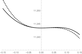
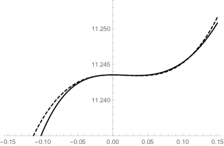
(a) $q=\alpha_{-}$, $\lambda=0.30449$           (b) $q=\alpha_{+}$, $\lambda=-0.448203$

Figure 10: Solid curve is $S(q+h\psi)$ against $h$ and $\psi$ its eigenfunction of $C_{e}$ at $T=T_{0}=14.4950$. (a) There is local minimum at $h=0$ and maximum at $h=0.0636$. (b) There is local maximum at $h=0$ and minimum at $h=0.0343$. Dashed curve is $S(q+h\psi)$ truncated at $h^{3}$ term (7).

In figure 10 (a) and (b), $S(q+h\psi)$ at $T=T_{0}$ for $\psi=C_{e}$ are plotted against $h$ for $q=\alpha_{-}$ and $\alpha_{+}$, respectively. In figure 10 (a), there are local minimum at $h=0$ due to $\lambda=0.30449>0$ and local maximum at $h=0.0636$, and in (b) local maximum due to $\lambda=-0.448203<0$ and local minimum at $h=0.0343$. Both $h$ are close to the distance between $\alpha_{-}$ and $\alpha_{+}$,

$$||q-q^{\prime}||=0.0428$$ (50)

where $q=\alpha_{-}$, $q^{\prime}=\alpha_{+}$, and $||f||=\sqrt{(f,f)}$, thus the local minimum and maximum at $h\neq 0$ are considered to be about the critical points corresponding to the solutions $\alpha_{+}$ and $\alpha_{-}$, respectively.

Dashed curves in figure 10 are $S(q+h\psi)$ truncated at $h^{3}$ term with $S^{(0)}=S(q)$, $S^{(1)}=0$, $S^{(2)}=\lambda$, $S^{(3)}=-2\lambda/h$ where $h$ in $S^{(3)}$ is given by (39). The positions of local maximum and minimum at $h\neq 0$ of dashed curves are calculated by (39) as $h=0.0466$ and $0.0384$, respectively. Here we have four values of $h$ distributed around (50) and one of them $h=0.0636$ for the local maximum in figure 10 (a) is deviated. The reason of this distribution is not yet understood.

In figure 8, (f), and in figure 1, (r) are the variated orbit for $C_{e}$. The former may represent $\alpha_{-}$ if $h$ is suitable, however, at present, the role of the latter for the homogeneous system is unknown.

We note that at the same $T$, $\alpha_{+}$ has higher action than $\alpha_{-}$ by definition, then as explained above, eigenvalue of the $C_{e}$ in $\alpha_{+}$ has to be negative and $\alpha_{-}$ positive in the vicinity of $T=T_{\min}$. In other words, following the solution $\alpha_{-}$ by decreasing $T$, its positive eigenvalue of $C_{e}$ has to change the sign negative at $T=T_{\min}$. Therefore all $N$, $N_{c}$ and $N_{e}$ have to jump by one at $T=T_{\min}$ as shown in figure 7.

4.3 Euler characteristic

We consider the action manifold $S(f)$ in the domain of the figure-eight choreographic function $f$ with period $T$ and its Euler characteristic

$$\chi_{e}=\sum_{q^{\prime}}(-1)^{N_{e}(q^{\prime})}$$ (51)

where $N_{e}(q^{\prime})$ is the Morse index at critical point $q^{\prime}$ of the manifold, that is, the figure-eight choreographic solution of (2). According to the theorem by Sbano and Southall [4], there is no figure-eight choreography with $T<T_{c}$ for some $T_{c}>0$, thus there is no critical point for $T<T_{c}$ then $\chi_{e}=0$. In the vicinity of $T=T_{\min}$, if there is no figure-eight choreography other than $\alpha$ as suggested in [5] where $T_{c}=T_{\min}$ is expected, we obtain the right hand side

$$(-1)^{0}+(-1)^{1}=0$$ (52)

by (46) and (49). This shows the relation (51) holds under a common assumption that the Euler characteristic $\chi_{e}$ is constant for $T>0$.

5 Summary and discussions

In this paper, we solved eigenvalue problem (13) for Morse indices numerically for the figure-eight choreographies under homogeneous potential with $a\geq 0$ and for the $\alpha$ solution under LJ potential (1).

The eigenfunctions are classified into periodic, choreographic, figure-eight choreographic, zero and trivial, and then three kind of Morse indices $N$, $N_{c}$ and $N_{e}$ are counted. We notice that the choreographic eigenfunction is non-degenerate and the non-choreographic eigenfunction is doubly degenerate. More detailed analysis of the operator $\hat{H}$ will be published elsewhere [11].

We then investigated the correlation of eigenfunctions in $T\geq T_{\min}$ for the solution $\alpha$ under LJ and in $a\geq 0$ for homogeneous system. For the two eigenfunctions, labeled $D_{y}^{H}$ and $C_{e}$, their variated orbits correspond to the real solutions, Simó’s H and the $\alpha$ solution itself, respectively.

Several questions arise on Simó’s H orbit. How does Simó’s H orbit change when $a$ is varied? Does periodic orbit corresponding to Simó’s H orbit exist for LJ system? Is there non-choreographic orbit corresponding to the $D$ with $\lambda=-0.0116029$ in figure 1 (a) and (b) for $a=1$, say, a non-symmetric H orbit since $D$ is not symmetric in $y$-axis? How does it behave at $a=a_{1}$ where the eigenvalue changes to positive?

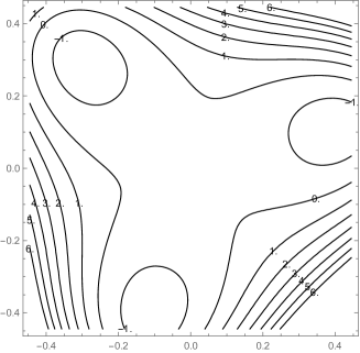
Figure 11: Contour plot for action $S(q+h\psi^{(\Theta)})$. $q$ is the figure-eight choreography under homogeneous potential with $a=a_{-}=0.994$ and the eigenfunction $\psi^{(\Theta)}$ at $s=3$ for $D_{y}^{H}$. Horizontal and vertical axis are $h\cos\Theta$ and $h\sin\Theta$, respectively. Contours are labeled by $(S(q+h\psi^{(\Theta)})-S(q))\times 10^{5}$.

At $a=a_{0}$, the eigenvalue of the $D_{y}^{H}$ correlated to the Simó’s H orbit changes the sign as (33). In figure 11, contour plot of the action $S(q+h\psi^{(\Theta)})$ for $\psi^{(\Theta)}=D_{y}^{H}$ at $a=a_{-}=0.994<a_{0}$ where eigenvalue for $D_{y}^{H}$ is negative are shown. The three fold symmetry and local minima around origin in contour is observed, suggesting the existence of Simó’s H orbit at $a=a_{-}$.

On the other hand, if there exists no Simó’s H at $a=a_{-}$, the Euler characteristic of the action manifold in the domain of the periodic function

$$\chi=\sum_{q^{\prime}}(-1)^{N(q^{\prime})}$$ (53)

at $a=a_{-}$ is $\chi=(-1)^{N}=(-1)^{4}=1$ by (33). However, at $a=1>a_{0}$, $\chi$ is even since $N=2$ by (33) and there are three critical points $q^{\prime}$’s for Simó’s H orbits, $(-1)^{2}+3(-1)^{N(q^{\prime})}=1\pm 3$. Thus the conservation of the Euler characteristic $\chi$ around $a=a_{0}$ also supports the existence of the Simó’s H at $a=a_{-}$. Then we expect that the Simó’s H orbit will exist in the both sides of $a=a_{0}$.

For the solution $\alpha$ under LJ potential, we found that Morse index $N_{e}$ for figure-eight choreography is 0 for $\alpha_{-}$ and 1 for $\alpha_{+}$ and that it changes at minimum of $T$. This behavior of $N_{e}$ is consistent with the Euler characteristic $\chi_{e}=0$ of the action manifold given by the theorem by Sbano and Southall [4]. We expect from this results that the calculation of Morse indices for the other series of solutions, $\beta$, $\gamma$, $\delta$, … found in [5] helps to understand their structures and relations through action manifold. Although we investigated what happened at zero of the eigenvalue for the eigenfunction $C_{e}$ under constant Euler characteristic $\chi_{e}$ in section 4.2 and 4.3, we did not for the other eigenfunctions yet: choreographic ones, $C$, $C_{y}$ and $C_{2}$ under $\chi_{c}=\sum_{q^{\prime}}(-1)^{N_{c}(q^{\prime})}$, and non-choreographic ones, $D_{y}^{H}$, $D_{y}$, $D$ and $D^{\prime}$ under $\chi=\sum_{q^{\prime}}(-1)^{N(q^{\prime})}$. They are also interesting and more studies will be needed in future.

The analysis in this paper was performed with a fixed value of the strength of the potential terms, (30), the repulsive term in the LJ potential (1) and the attractive. However, since the changes of the strength of potential terms are identical to the scale transformation in time and length, the analysis is not changed if the strength is varied.

References

References

- [1] Moore C, 1993 Braids in Classical Gravity, Phys. Rev. Lett. 70, 3675–3679
- [2] Chenciner A and Montgomery R 2000 A remarkable periodic solution of the three-body problem in the case of equal masses, Annals of Mathematics 152, 881–901
- [3] Sbano L 2005 Symmetric solutions in molecular potentials, Proceedings of the international conference SPT2004, Symmetry and perturbation theory, (World Scientific Publishing, Singapore) 291–299.
- [4] Sbano L and Southall J 2010 Periodic solutions of the N-body problem with Lennard-Jones-type potentials, Dynamical Systems 25, 53–73
- [5] Hiroshi Fukuda, Toshiaki Fujiwara, Hiroshi Ozaki, Figure-eight choreographies of the equal mass three-body problem with Lennard-Jones-type potentials, J. Phys. A: Math. Theor. 50, 105202 (2017).
- [6] Shibayama, Numerical calculation of the second variation for the choreographic solution, in Japanese, Computations and Calculations in Celestial Mechanics Proceedings of Symposium on Celestial Mechanics and -body Dynamics, (2010) Eds. M. Saito, M. Shibayama and M. Sekiguchi.
- [7] Vivina Barutello, Riccardo D. Jadanza, Alessandro Portaluri, Morse index and linear stability of the Lagrangian circular orbit in a three-body-type problem via index theory, A. Arch Rational Mech Anal (2016) 219: 387.
- [8] Xijun Hu and Shanzhong Sun, Morse index and stability of elliptic Lagrangian solutions in the planar three-body problem, Advances in Mathematics, 223 98–119, (2010).
- [9] Hu, X. and Sun, S. Index and Stability of Symmetric Periodic Orbits in Hamiltonian Systems with Application to Figure-Eight Orbit, Commun. Math. Phys. (2009) 290: 737.
- [10] Simó C, Dynamical properties of the figure eight solution of the three body problem, Proceedings of the Celestial Mechanics Conference dedicated to D. Saari for his 60th birthday, Evanston, ed. A. Chenciner et al, Contemporary Mathematics 292, pp. 209–228, 2000.
- [11] Fujiwara T, Fukuda H and Ozaki H Decomposition of the Hessian matrix for action at choreographic three-body solutions, will be published elsewhere.