The photon-index - time-lag correlation in black-hole X-ray binaries

Abstract

We have performed a timing and spectral analysis of a set of black-hole binaries to study the correlation between the photon index and the time lag of the hard photons with respect to the soft ones. We provide further evidence that the timing and spectral properties in black-hole X-ray binaries are coupled. In particular, we find that the average time lag increases as the X-ray emission becomes softer. Although a correlation between the hardness of the X-ray spectrum and the time (or phase) lag has been reported in the past for a handful of systems, our study confirms that this correlated behaviour is a global property of black-hole X-ray binaries. We also demonstrate that the photon-index - time-lag correlation can be explained as a result of inverse Comptonization in a jet.

Table 1: List of sources. The fifth column gives the final number of observations used (blue empty circles in Fig. 2) over the total number analysed.

Object	Outburst	MJD interval	Total exposure	Observations
	epoch		time (ks)	lags/total
4U 1543–475	2002	52443–52565	275.4	16/106
Cyg X–1	2003-2004	52693–53182	367.4	135/151
GRO J1655–40	2005	53423–53685	2238.3	66/501
GX 339–4	2002	52311–52884	495.6	45/267
	2004	53050–53498	565.2	139/328
	2007	53769–54678	572.6	177/347
H 1743–322	2008	54746–54789	66.3	34/182
	2009	54980–55039	84.9	16/182
XTE J1720–318	2003	52654–52849	261.9	32/99
XTE J1550–564	2000	51644–51741	128.7	25/66
	2001–2004	51938–53163	306.5	64/101
XTE J1650–500	2002	52159–52447	327.9	46/182

1 Introduction

The vast majority of black-hole binaries (BHBs) are transient X-ray sources that spend much of their life in a dormant state. Occasionally, they become the brightest sources of the X-ray sky. The X-ray outbursts last from weeks to months and are characterized by a fast rise and a slower decay, although there is no unique morphological type (Chen et al., 1997). During these outbursts, the timing and spectral properties change, defining a series of states. In a plot of X-ray luminosity (or count rate) as a function of hardness, the so-called hardness-luminosity (HLD) or hardness-intensity diagram (HID), the sources trace a characteristic $q$-shaped pattern, where each state occupies a specific part of the diagram (e.g. Kylafis & Belloni, 2015a, b, and references therein).

The physical processes that give rise to the X-ray emission are thermal and non-thermal. When the flux is high, the X-ray spectrum is dominated by a thermal component that is generally modeled as a multi-temperature blackbody with a characteristic temperature of 0.1–0.5 keV. The origin of this component is believed to be the innermost part of a geometrically thin, optically thick accretion disk (Shakura & Sunyaev, 1973), which is formed by mass transfer from the optical companion through the Lagrangian point of the Roche lobe. When the flux is low, the X-ray spectrum is dominated by a non-termal component, which is best described as a power law with an exponential cutoff. The origin of this component is believed to be inverse Compton scattering of low-energy photons off very energetic electrons. However, neither the origin of the photons that are up-scattered nor the geometry and properties of the comptonizing medium are known with certainty. The Comptonizing medium could be an optically thin, very hot "corona" in the vicinity of the compact object (Sunyaev & Titarchuk, 1980; Hua & Titarchuk, 1995; Zdziarski, 1998), an advection-dominated accretion flow (Narayan & Yi, 1994; Esin et al., 1997), a low angular momentum accretion flow (Ghosh et al., 2011; Garain et al., 2012), the base of a radio jet (Band & Grindlay, 1986; Georganopoulos et al., 2002; Markoff et al., 2005) or a more extended jet (Reig et al., 2003; Giannios, 2005). The most likely origin for the source of low-energy photons is the blackbody photons from the accretion disk. Other possible scenarios involve cosmic microwave background photons or synchrotron photons emitted by jet electrons (Giannios, 2005; McNamara et al., 2009).

Because the blackbody emission is at low energies and power-law emission at high energies, the states where these components are dominant are called soft and hard, respectively. The power-law spectrum observed in the hard state is commonly referred to as the hard tail.

Optically thick, compact, steady radio emission is detected during the hard state, while optically thin radio flares occur during transitions from the hard to the soft sate. The association of compact radio jets and X-ray hard tails with a specific region of the source in the hardness-intensity diagram is well documented (Fender et al., 2004; Migliari & Fender, 2006; Migliari et al., 2007; Fender et al., 2009; Miller-Jones et al., 2010). Both the radio emission and the strength of the hard tail become weaker at higher accretion rates. Radio and hard X-rays show the strongest intensity in the hard states of BHBs. For the formation and destruction of jets in black-hole and neutron-star binaries, the reader is referred to Kylafis et al. (2012).

Spectral information alone cannot reveal the accretion geometry: different models can result in very similar energy spectra (Nowak et al., 2011). Significant advances in our understanding of how the X-ray mechanism in BHBs works can be achieved when we combine variability and spectral information. The discovery of correlations between a) the characteristic frequencies of the noise components in the power spectra and the photon index of the power-law in the energy spectra (Di Matteo & Psaltis, 1999; Shaposhnikov & Titarchuk, 2009; Shidatsu et al., 2014), b) the broad-band noise components with luminosity (Reig et al., 2013), c) the broad-band noise components with the disk temperature and radius (Kalamkar et al., 2015), d) the photon index with the time lag (Pottschmidt et al., 2003; Grinberg et al., 2014), and the anticorrelations e) between the fraction of up-scattered photons and the characteristic frequency of quasi-periodic oscillations (QPO) (Stiele et al., 2013), and f) between the cut-off energy and the phase lag (Altamirano & Méndez, 2015; Reig & Kylafis, 2015) constitute convincing evidence that the timing and spectral properties of the sources are closely linked. In particular, the time lag between two different energy bands sets tight constraints on the models of the X-ray production. In most cases, positive lags, i.e. hard photons delayed with respect to soft photons, are observed. The lag follows a power-law dependence with Fourier frequency $\tau\propto\nu^{-0.8\pm 0.1}$ (Crary et al., 1998; Nowak et al., 1999; Cassatella et al., 2012). Positive lag calculated at energies above $\sim$2 keV has been traditionally attributed to inverse Comptonization. In order to acquire their energy, harder photons scatter more times than softer photons, hence staying longer in the Comptonizing medium before they escape. In this context, time lags simply signify the light-travel time of photons within the Comptonizing region. A different explanation of the time lags was offered by Kotov et al. (2001) and Arévalo & Uttley (2006). In their model, the lags result from viscous propagation of mass accretion fluctuations within the inner regions of the disk.

In this work, we focus on the correlation between the shape of the spectral continuum and the time lag in the hard state by analysing data corresponding to twelve outbursts of eight BHBs. So far, this correlation has been reported in detail for Cyg X-1 (Pottschmidt et al., 2003; Böck et al., 2011; Grinberg et al., 2014) and GX 339–4 (Nowak et al., 2002; Altamirano & Méndez, 2015). A decrease of the time lag as the source spectrum becomes harder has also been observed in XTE J1650–500 (Kalemci et al., 2003) and 4U 1543-47 (Kalemci et al., 2005). Kalemci (2002) combined observations from several systems into one diagram, highlighting the fact that this correlation may be a common feature in BHBs. Our results confirm the universality of the correlation.

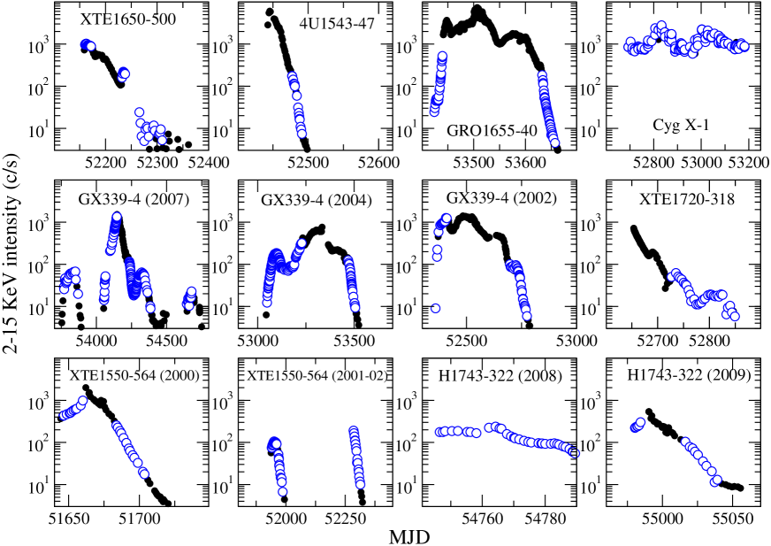
Figure 1: Light curves. Each point corresponds to one observation. The blue empty circles identify the observations used in the final lag-spectral analysis.

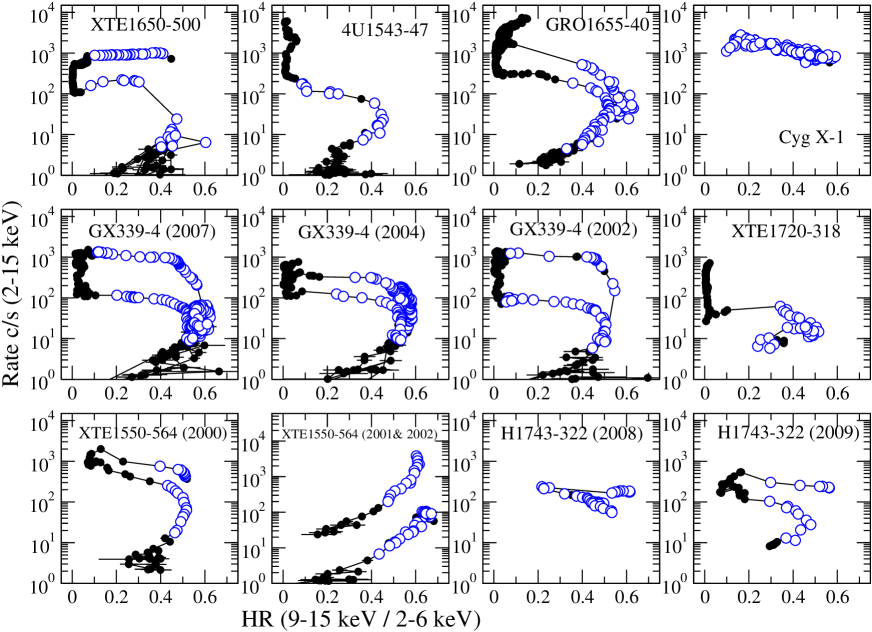
Figure 2: Hardness-intensity diagrams. Each point corresponds to one observation. The blue empty circles identify the observations used in the final lag-spectral analysis. We show two mini-outbursts of XTE J1550–564 in the same panel. The 2002 points were shifted up ($\times$ 20) for clarity.

2 Observations and data analysis

All the observations of the sources analyzed in this work (Table 1) are available in the Rossi X-ray Timing Explorer (RXTE) archive. All these sources (except for Cyg X–1, see e.g. Grinberg et al. 2013) are X-ray transients, that are only detected when they undergo an outburst. During the outburst, the X-ray luminosity increases by three or four orders of magnitude. We have also included Cyg X–1 because it is the best studied BHB and will allow us to verify our results with previous work. The sample of sources is not intended to be complete. We selected sources with well-sampled outbursts.

The RXTE mission was operational in the period 1996–2012 and carried three detectors: the Proportional Counter Array (PCA), the High-energy X-ray Experiment (HEXTE), and the All Sky Monitor (ASM). The PCA (Jahoda et al., 2006) covered the energy range 2–60 keV and consisted of five identical coaligned gas-filled proportional units (PCU), giving a total collecting area of 6500 cm² and provided an energy resolution of 18% at 6 keV. The HEXTE (Rothschild et al., 1998) was constituted of 2 clusters of 4 NaI/CsI scintillation counters each, with a total collecting area of 2 $\times$ 800 cm², sensitive in the 15–250 keV band, with a nominal energy resolution of 15% at 60 keV. The ASM (Levine et al., 1996) scanned about 80% of the sky every orbit, allowing monitoring on time scales of 90 minutes or longer in the energy range 1.3–12.1 keV.

Due to RXTE’s low-Earth orbit, the observations consisted of a number of contiguous data intervals or pointings interspersed with observational gaps produced by Earth occultations of the source and passages of the satellite through the South Atlantic Anomaly. Data taken during satellite slews, passage through the South Atlantic Anomaly, Earth’s occultation, and high voltage breakdown were filtered out. Typically, an observation consists of a continuous stretch of data with a duration of 1000–3000 seconds, although shorter and longer duration intervals are present in the data.

The timing analysis was performed using data from all the PCUs, except when a comparison of the intensity levels was relevant (e.g. Fig. 2), in which case we used PCU2 because it was the best calibrated PCU and the one that was in operation all the time. The spectral analysis was performed using data from the PCU2 and HEXTE. We used Clusters A and B until July 2006, when the detector’s on- and off-source modulation of cluster A began to experience problems, and Cluster B only from that period until December 2010 when it suffered the same malfunction. Owing to these problems, we did not analyse data after December 2010.

2.1 Timing analysis

The timing analysis consisted of the extraction of light curves, which allowed us to examine the outburst profiles and compute the power spectral density (PSD) and the time lag. The light curve was divided into 64-s segments and a Fast Fourier Transform was computed for each segment. The final power spectrum is the average of all the power spectra obtained for each segment. The power spectra were logarithmically rebinned in frequency and normalized such that the integral gives the squared rms fractional variability (Belloni & Hasinger, 1990; Miyamoto et al., 1991). A multicomponent model, consisting of three Lorentzian functions, fit most of the PSD adequately. When a strong quasi-periodic oscillation (QPO) was present, then another Lorentzian component was added. We fitted the PSD for the only purpose to calculate the broad-band (0.01–30 Hz) rms to select the hard states.

We computed the time lag between photons in the energy range 9–15 keV (hard band) with respect to the reference band 2–6 keV (soft band) for each observation interval. We generated light curves $x_{i}(t)$ with time bin size $2^{-7}$ s for each of these two bands. Each light curve was divided into 64-s segments and its Fourier transform $X_{i}(\nu_{j})$ was computed for each segment. The Fourier transforms were used to compute the average cross-spectrum, defined as $C(\nu_{j})=X_{1}^{*}(\nu_{j})X_{2}(\nu_{j})$, where the asterisk denotes complex conjugate. The phase lag between the signals in the two bands at Fourier frequency $\nu_{j}$ is $\phi(\nu_{j})=arg[C(\nu_{j})]$ [the position angle of $C(\nu_{j})$ in the complex plane] and the corresponding time lag $t_{\rm lag}(\nu_{j})=\phi(\nu_{j})/2\pi\,\nu_{j}$. We calculated an average cross vector $<C(\nu_{j})>$ by averaging the complex values over multiple adjacent 64-s spectra at each frequency. The final time lag resulted from the average of the time lags in the frequency range 0.05–5 Hz.

Figure 3: Distribution of the reduced $\chi^{2}$ after fitting the spectra with the broken power law model.

2.2 Selection of the hard state

In this work we are interested in the hard and hard-intermediate states of BHBs, because these are the states when inverse Comptonization dominates the X-ray emission. We identified the hard and hard-intermediate states using timing information only. By ignoring spectral information, we avoid the introduction of possible bias in the selection procedure, as our objective is to investigate the relationship between timing and spectral parameters.

Hard states are characterised by strong variability of the form of band-limited noise (Muñoz-Darias et al., 2011; Belloni et al., 2011). As representative of the hard and hard-intermediate states, we selected observations with an rms above 10%. The rms was obtained from the 2–15 keV PSD in the frequency range 0.01–30 Hz. To have an acceptable signal-to-noise, we discarded observations with less than 20 c s^-1 in the 2–30 keV range. Likewise, we only considered observations that contain at least ten data segments of 64-s length each.

To better visualize the selected data, we show the outburst light curves in Fig. 1 and the hardness-intensity diagrams (HID) in Fig. 2. To create the HID, we extracted light curves with a time resolution of 16 s using the Standard 2 configuration in three different energy bands. We used the counts in the energy ranges 2–6 keV and 9–15 keV to derive the hardness ratio HR, while the intensity (Y-axis) corresponds to the energy range 2–15 keV. We obtained one point per observation by averaging the count rate of the corresponding light curve. In Figs. 1 and 2, we indicate with circles (filled and empty) all the observations initially considered (Table 1). With blue empty circles we display the observations selected for further analysis, that is those observations that fulfill the selection criteria stated above. As can be seen in Fig. 2, our selection criteria based solely on the timing properties result in observations that correspond to hard and intermediate states and do not include observations in the soft state, that is, points in the vertical left branch of the HID.

XTE J1550–564 (and H 1743–322) sometimes displays mini-outbursts with low but significant increases in intensity above the quiescent state. In these mini-outbursts the source remains in the hard state and does not show state transitions. Two of these mini-outbursts of XTE J1550–564 have been plotted in the same panel in Fig. 2. In this panel, we shifted up ($\times 20$) the data points of the 2002 outburst for clarity.

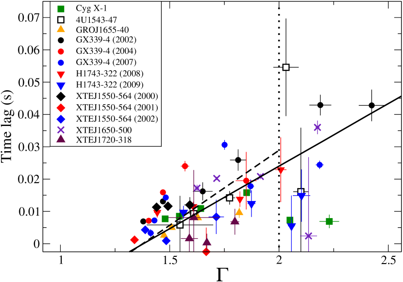
Figure 4: The correlation between the photon index, $\Gamma$, and the average time lag, for all observations. Each point is the average of the observations within a bin in HR of size 0.1. in The time lag was obtained between the 9–15 keV photons and 2–6 keV photons and averaged in the frequency range 0.05–5 Hz. The solid line is the fit to all data points while the dashed line is the fit to points with $\Gamma<2$.

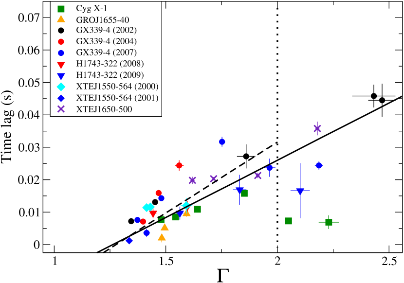
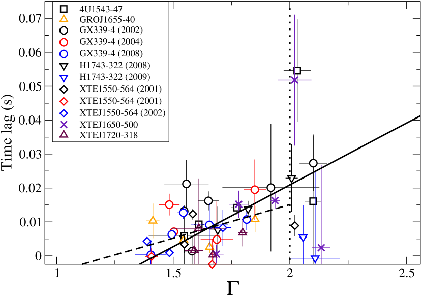
Figure 5: The correlation between the photon index, $\Gamma$, and the average time lag, considering only observations during the rise (left) and the decay (right) of the outburst. The solid line is the fit to all data points while the dashed line is the fit to points with $\Gamma<2$.

2.3 Spectral analysis

For the selected observations, we obtained the energy spectra using the standard modes for both PCA and HEXTE. PCA provides 128 channels, while HEXTE provides 64 channels to cover the full energy range. The PCA spectrum becomes background dominated above $\sim 25$ keV, while the calibration below $\sim 3$ keV is uncertain. Because the hard state is a low-intensity state, the HEXTE spectra begin to be dominated by the background at higher energies. Therefore the overall energy range considered in our spectral analysis was 3–150 keV.

We wished to characterise the spectral continuum dominated by Comptonization in as much an independent way as possible, regardless of the underlying physical process. For this reason, we chose the photon index of a power-law model to be representative of this component. Thus, we first fitted the spectra with a simple model that consisted of an absorbed power law and an exponential cutoff. A narrow Gaussian component (line width $\sigma\mathbin{\lower 3.0pt\hbox{$\hbox to0.0pt{\raise 5.0pt\hbox{$\char 60\relax$}\hss}\mathchar 29208\relax$}}0.9$ keV) was added to account for the iron emission line at around 6.4 keV. The hydrogen column density was fixed to the values provided by Dunn et al. (2010). For Cyg X–1 we used the value given by Hanke et al. (2009). This model left significant residuals below 10 keV. Substantial improvement was achieved with the use of a broken power-law model. Figure 3 shows the distribution of the reduced $\chi^{2}$. The distribution peaks at around 1. The reduced $\chi^{2}$ of 85% of the fits lie in the range $0.7\leq\chi^{2}\leq 1.3$, while 91% of the observations have $0.7\leq\chi^{2}\leq 2$. The broken power-law model has been successfully used to fit the spectra of Cyg X–1 (Wilms et al., 2006; Grinberg et al., 2014). The parameters of the broken power-law model are a soft photon index, a hard photon index, and a break energy. The break energy is typically found at $\sim 10$ keV. We used the best-fit hard photon index in our analysis. In some sources, the X-ray continuum shows a roll over at high energy, which was modeled with an exponential cutoff. As expected, no blackbody component was needed to obtain a good fit.

Table 2: Results of the linear regression and correlation analysis for all $\Gamma$ and for $\Gamma<2$. Here $r$ is Pearson’s correlation coefficient, $N$ is the number of points, and $p$ the probability that the null hypothesis (no correlation) is true.

	All points					Points with $\Gamma<2$
	Intercept	Slope	$r$	N	$p$-value	Intercept	Slope	$r$	N	$p$-value
All	$-0.053\pm 0.012$	$0.039\pm 0.008$	0.57	57	$4.5\times 10^{-6}$	$-0.064\pm 0.016$	$0.046\pm 0.010$	0.51	45	$3.6\times 10^{-4}$
Rise	$-0.045\pm 0.004$	$0.035\pm 0.003$	0.73	37	$3.6\times 10^{-7}$	$-0.056\pm 0.010$	$0.044\pm 0.007$	0.72	30	$7.0\times 10^{-6}$
Decay	$-0.052\pm 0.033$	$0.036\pm 0.020$	0.44	47	$1.9\times 10^{-3}$	$-0.025\pm 0.025$	$0.020\pm 0.016$	0.36	39	$2.6\times 10^{-2}$

3 Results

Figure 4 shows the average time lag as a function of the photon index. In this figure, we rebinned the observations according to their position in the HID (Fig. 2), i.e. we divided the $HR$ range from 0.0 to 0.7 into bins of size 0.1 and obtained the weighted average time lag and photon index in the corresponding bin. Thus each point in Fig. 4 is the average of a varying number of observations. If the average is formed out of two points, then the error is obtained as $\sigma=(\sigma_{1}^{2}+\sigma_{2}^{2})^{1/2}$, where $\sigma_{1}$ and $\sigma_{2}$ are the individual errors of the two points. When the bin contains only one point, we retained the original error. To study the posibility of different behaviour during the rise and the decay of the outbursts, we selected observations corresponding to each one of these two cases separately, and rebinned them as before. The relationship between the time lag and the photon index for the rise and decay is shown in Fig. 5.

Although these figures exhibit large dispersion, there is a general trend showing that the time lag increases as the photon index increases. For $\Gamma\mathbin{\lower 3.0pt\hbox{$\hbox to0.0pt{\raise 5.0pt\hbox{$\char 62\relax$}\hss}\mathchar 29208\relax$}}2$, that is when the source leaves the pure hard state and enters the hard-intermediate state, before crossing the jet line, the relationship becomes more complex, with some sources showing a reversed trend, i.e. the lags decrease when the photon index increases. This behaviour is well documented in Cyg X–1 (Grinberg et al., 2014). Not all the sources show a turning point, but this might be due to the fact that different sources may reach the soft state at different $\Gamma$. Even different outbursts of the same source may or may not show the drop in $t_{\rm lag}$ at larger $\Gamma$, as in GX 339–4 (Altamirano & Méndez, 2015).

We now investigate whether the observed trend between the photon index and the time lag is statistically significant by performing a correlation and a linear regression analysis on the three groups of points considered, namely the whole sample (Fig. 4) and the rise and decay of the outburst (Fig. 5), separately. In addition, for each one of these three groups, we carry out the analysis considering all data points and those with $\Gamma<2$. The latter case would correspond to a pure hard state. The results are presented in Table 2. First, we study whether the two variables correlate by computing the Pearson’s correlation coefficient, $r$, and the probabilty of the null hypothesis, $p$-value, i.e. that there is no correlation between the two variables. We find a significant positive correlation ($r=0.57$) when we consider all data points (Fig. 4). The correlation becomes stronger ($r=0.73$) when we consider the points during the rise phase of the outbursts (left panel of Fig. 5). During the decay (right panel of Fig. 5), the correlation is weaker ($r=0.44$) than in the other two cases. The positive correlation remains strong when we consider the rise points with $\Gamma<2$ (left panel in Fig. 5), despite the fact that the number of points is smaller. In contrast, an even weaker correlation is found for the decay data set and $\Gamma<2$.

We also performed a linear fit to the data. There is no apriori reason to choose one of the two variables as the independent variable. The lags and the photon index are not directly correlated in the sense that one can be considered the cause and the other one the effect. The correlation between time lag and spectral continuum most likely arises because the two variables correlate with another unknown physical parameter (e.g. optical depth, accretion rate). Moreover, the intrinsic scatter of the data dominates over the errors arising from the observations and the measurement process. Under these circumstances, the preferred linear regression method is the bisector of the two lines that correspond to the least-square fit of Y on X and X on Y following the prescription by Akritas & Bershady (1996), which takes into account both the individual errors and the intrinsic scatter. The linear regression is shown in Figs. 4 and 5 as solid lines (all $\Gamma$) and dashed lines ($\Gamma<2$) and the results are presented in Table 2.

When we include points in both the hard and hard-intermediate states, i.e. all $\Gamma$, the slope of the regression is not consistent with zero, irrespective of the phase of the outburst, although for the decay data, the slope deviates from zero at less than $2\sigma$. When we consider points with $\Gamma<2$, the slopes of the data sets that include the entire outburst and that of the rise are steeper than when all $\Gamma$ are considered. In contrast, that of the decay group is flatter. However, we notice that the slope of the three groups is consistent within errors with the values when all data points are taken into account.

The extrapolation of the best-fit values for $\Gamma\mathbin{\lower 3.0pt\hbox{$\hbox to0.0pt{\raise 5.0pt\hbox{$\char 60\relax$}\hss}\mathchar 29208\relax$}}1.2$ predicts negative lags (Figs. 4 and 5), which is at odds with Comptonization models. In terms of the outburst evolution, such extrapolation would mean entering the quiescent state. However, studies of the quiescent state of BHBs show that as the systems fade from the low/hard state toward quiescence, their X-ray spectra become softer with typical values of $\Gamma$ in the range 2–3 (Tomsick et al., 2001, 2004; Kalemci et al., 2005; Wu & Gu, 2008; Sobolewska et al., 2011; Armas Padilla et al., 2013). Thus, the correlation must break down at around $\Gamma\sim 1.2$.

Our results can be summarised as follows: i) we detect a significant and strong positive correlation between time lag and spectral slope during the rise phase of the outbursts in BHBs. ii) The significance of the correlation is lower during the decay. This may simply be a consequence of the poorer statistics as a result of lower count rates. During the decay, the X-ray intensity is typically an order of magnitude lower than during the rise. iii) The correlation does not change significantly when we consider observations with $\Gamma<2$ only, and iv) the correlation breaks down when the source enters the quiescent state.

Next, we investigate whether Comptonization in a jet can explain these results.

4 A jet model

All BHBs show radio emission that points toward evidence of the presence of a compact radio jet when they are in their quiescent, hard, and hard-intermediate states (Fender & Belloni, 2012). Over the years we have developed a jet model to explain the spectral and timing properties of BHBs (Reig et al., 2003; Giannios et al., 2004; Giannios, 2005; Kylafis et al., 2008; Reig & Kylafis, 2015).

The jet model used here is the same as the one used in Reig & Kylafis (2015), which in turn, is based on the model described in Kylafis et al. (2008), with the addition of an acceleration zone. The jet has an acceleration region of height $z_{1}$ beyond which the flow has a constant velocity equal to $v_{0}$. Hence, the flow velocity in the jet is given by

$$v_{\parallel}(z)=\begin{cases}(z/z_{1})^{p}~{}v_{0}&\text{if }\,\,\,0<z\leqslant z_{1}\\ v_{0}&\text{if}\,\,\,\,\,z>z_{1}\end{cases}$$ (1)

The radius of the jet at height $z$ is $R(z)=R_{0}(z/z_{0})^{1/2}$, which corresponds to a parabolic jet. The density outside the acceleration region is $n_{e}(z)=n_{0}(z_{0}/z)$. Within the acceleration region, the density is obtained through the continuity equation $n_{\rm acc}(z)=(z_{1}/z)^{p}\,\,n_{e}(z)$.

The parameters of the model are: the optical depth along the jet’s axis $\tau_{\parallel}$, the width of the jet at its base $R_{0}$, the parallel, $v_{0}$, and perpendicular, $v_{\perp}$, components of the velocity, or equivalently the Lorentz factor $\gamma=1/\sqrt{1-(v_{0}^{2}+v_{\perp}^{2})/c^{2}}$, the distance $z_{0}$ of the bottom of the jet from the black hole, the total height $H$ of the jet, the size $z_{1}$ and exponent $p$ of the acceleration zone, and the temperature $T_{bb}$ of the soft-photon input. Our assumption of a characteristic Lorentz $\gamma$ in the flow is equivalent to considering the smallest Lorentz factor of a steep power-law distribution (Giannios et al., 2004; Giannios, 2005).

Physically, a variation in optical depth is equivalent to a change in the density at the base of the jet. Hence, $\tau_{\parallel}$ is the prime parameter that drives the changes in the photon index. A change in $R_{0}$ corresponds to a change in the size of the jet, and time lags are strongly affected by changes in $R_{0}$. Finally, the variation in $v_{\perp}$ (or $\gamma$) mimics the process of Compton cooling, which is related to the cutoff at high energy.

The top panel of Fig. 6 shows the $\Gamma$–$t_{\rm lag}$ correlation for different models. The empty red circles correspond to pairs of the model parameters $\tau_{\parallel}$ and $R_{0}$, with constant $\gamma=2.24$. This value of $\gamma$ was chosen because it matches the cutoff energy of $\sim 100$ keV, observed in GX 339–4 (Motta et al., 2009). The parameters varied in the ranges $2\leqslant\tau_{\parallel}\leqslant 11$ and $40\leqslant R_{0}/r_{g}\leqslant 900$, where $r_{g}=GM/c^{2}$ is the gravitational radius of the black hole. The models (empty red circles) were selected to match the best-fit line to the data (left panel in Fig. 5). Figure 6, bottom panel, displays the data shown in the left panel of Fig. 5 and the solid line of Fig. 6, top panel., which in this case, is the best-fit line to the models. Similarly, we computed pairs $(\Gamma,~{}t_{\rm lag})$ keeping $R_{0}$ constant at two different values: $R_{0}=100r_{g}$ (empty blue squares) and $R_{0}=300r_{g}$ (filled green squares) in Fig. 6, top panel. In these two cases, we varied the model parameters $2\leqslant\tau_{\parallel}\leqslant 11$ and $2.0\leqslant\gamma\leqslant 2.8$. The dotted line is the best linear fit to the $R_{0}=100r_{g}$ models and the dashed line to the $R_{0}=300r_{g}$ ones. In all the models, the rest of the parameters are fixed at the following reference values: $z_{0}=5r_{g}$, $H=10^{5}r_{g}$, $v_{0}=0.8c$, $z_{1}=50r_{g}$, $p=0.5$, and $T_{bb}=0.2$ keV.

We can reproduce the $\Gamma$ - $t_{\rm lag}$ correlation by changing the width of the jet at its base and the optical depth along the jet’s axis. In contrast, we cannot reproduce the correct slope with a fixed width at the base of the jet. Changing the optical depth and the perpendicular component of the jet velocity, without changing the width of the jet can reproduce the range of photon index, but not the range of time lag.

We also find that to explain the $\Gamma$ - $t_{\rm lag}$ correlation, $\tau_{\parallel}$ and $R_{0}$ should vary in a highly correlated way following a power-law function, $\tau_{\parallel}\propto R_{0}^{\alpha}$ with index $\alpha=-0.57$ (Fig. 7). This index is smaller than the one found in Kylafis et al. (2008) for Cyg X–1. The difference can be attributed to the acceleration region, which was absent in Kylafis et al. (2008). The acceleration zone was introduced to explain the correlation between the cut-off energy and phase lags in GX 339–4 (Reig & Kylafis, 2015). As shown in Reig & Kylafis (2015), for a given value of $\tau_{\parallel}$, the models with the acceleration zone produce shorter lags than when acceleration occurs instantaneously. The natural way to increase the lags is by increasing the size of the jet.

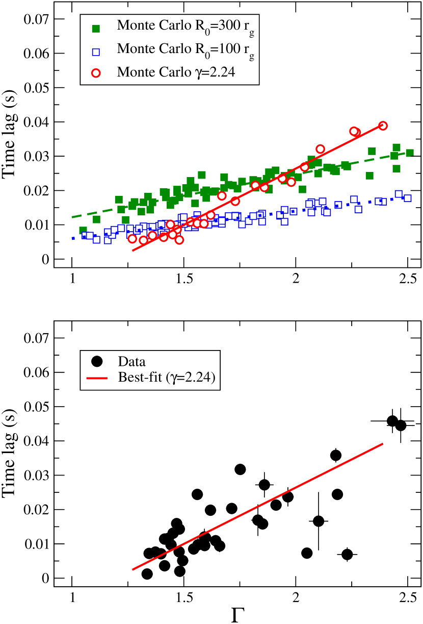
Figure 6: The correlation between the photon index, $\Gamma$, and the average time lag. In the upper panel, the points correspond to different jet models obtained from Monte Carlo simulations with a fixed value of the Lorentz factor $\gamma$ and variable width at the base of the jet $R_{0}$ (circles) and fixed $R_{0}$ and variable $\gamma$ (squares). The lines represents the best linear fit to the points. In the bottom panel, the observational data (circles) from the left panel of Fig. 5 and the best-fit from the Monte Carlo simulation (solid line in the upper panel) are plotted together.

5 Discussion

Extensive studies of Cyg X–1 (Nowak et al., 2002; Pottschmidt et al., 2003; Böck et al., 2011; Grinberg et al., 2014) and GX 339–4 (Altamirano & Méndez, 2015) have shown that the time lag increases with decreasing hardness, that is, as the source transits from the hard to the intermediate state. A similar behaviour has been reported for XTE J1650-500 (Kalemci et al., 2003) and 4U 1543-47 (Kalemci et al., 2005). Our study reveals that this correlated behaviour is a global property of BHBs. The $\Gamma$ - $t_{\rm lag}$ correlation imposes stringent constraints on all the models that seek to explain the behaviour of BHBs. A model that can successfully explain the time delay between two energy bands, should also predict the right spectrum.

In Comptonization models, the lags are related to the average number of scatterings of the low-energy photons with highly energetic electrons. Hence, the time lag is related to a characteristic length scale of the medium which upscatters the observed photons. Nowak et al. (2002) modeled the spectrum of GX 339–4 with a hybrid coronal model and found that higher coronal compactness, defined as the energy released by the Comptonizing medium divided by its radius (see Coppi, 1999, for a review), is associated with shorter time lags. The higher the compactness parameter, the harder the spectra. In principle, compactness changes are achieved solely by varying the coronal radius. A large corona would be associated with high compactness, i.e., harder spectra, but also, following the geometric interpretation, with larger lags, contrary to what is observed. Nowak et al. (2002) suggested a jet-like model, where the corona is simply the base of the jet. The correlation between compactness and lags in GX 339–4 was observed when the source went from the soft to the hard state. This transition would be associated with the formation of a jet. Time lags could be generated via propagation along the length of the jet.

Alternatively, Kalemci (2002) explained the correlation by invoking a hotter medium (“corona") in the hard state, and a cooler one as the source transits to the soft state. In a very hot medium, the time lag becomes insignificant because the number of scatterings is roughly the same independent of the energy. The problem with a uniform static corona is the lack of a heating mechanism to maintain a highly energetic electron population away (hundreds of gravitational radii) from the black hole as required by the magnitude of the observed lags ($\sim 0.1$ s).

In this work we demonstrate that Comptonization in the jet can reproduce satisfactorily the observed relationship between the X-ray spectral continuum emission and the time lag of hard photons with respect to softer ones. In fact, the correlation between the photon index and the time lag suggests that the lag originates in the jet, that is, the same region as where the hard X-rays are formed. The identification of the Comptonizing medium is a matter of intense debate with corona, ADAF, and jet as the prime candidates. The fact that the lags disappear or decrease abruptly when the source moves to the soft state, i.e., when the radio emission weakens, strongly supports a jet model.

To understand how Comptonization in the jet can explain the time-lag - photon-index correlation, we need to understand the dependence of the lags and the photon index on the main parameters of the jet, $\tau_{\parallel}$, $R_{0}$, and $\gamma$. At high optical depth, the disk photons penetrate the base of the jet superficially. Because of the high density, the mean free path is short and the photons sample a small region at the base of the jet before they escape. The photon suffers a large number of scatterings on short length scales. Thus the time lag between hard and softer photons is small and the spectrum is hard (small $\Gamma$). As the optical depth (or equivalently the density) decreases, the mean free path increases, and the photons sample a larger volume of the jet. Thus, the time lag increases and the spectrum becomes softer (larger $\Gamma$). For the same reasons, as $R_{0}$ increases while keeping $\tau_{\parallel}$ constant, the lags increase and the photon index decreases (Reig et al., 2003), i.e. the photons sample a larger volume and more scatterings take place in a larger jet. The scatter in the $\Gamma$ - $t_{\rm lag}$ correlation could then be related to differences in the jet’s characteristics such as optical depth, size, and/or velocity.

The X-ray spectral continuum of some sources displays an exponential cutoff in the hard state. The value $E_{\rm cut}$ varies from source to source in the range $\sim$50–200 keV. In our jet model, the cutoff energy strongly depends on the parameter $\gamma$ (Lorentz factor), i.e. the perpendicular component of the jet velocity, because it determines the maximum energy gain by the soft photons (Giannios et al., 2004). In this work we find that the $\Gamma$ - $t_{\rm lag}$ correlation can be reproduced with different fixed values of $\gamma$. All the sets of models displayed in Fig. 7 reproduce the $\Gamma$ - $t_{\rm lag}$ correlation satisfactorily. If we plotted the corresponding lines in the bottom panel of Fig. 6, they would differ by less than  1-2 line widths. Figure 7 shows that for a given $\tau_{\parallel}$, wider jets are required at lower velocities. Interestingly, the slope $\alpha$ of the relation between $\tau_{\parallel}$ and $R_{0}$ remains the same, irrespective of the value of $\gamma$. We conclude that the differences observed in the cutoff energy can be explained by invoking differet jet velocity. We refer the reader to Reig & Kylafis (2015) for a study of the dependence of the cutoff energy with $\gamma$.

In previous work, we have shown that Comptonization of low-energy disk photons by energetic electrons in a jet can reproduce many of the timing and spectral properties of BHBs in the hard state. By changing a small number of the parameters of the jet such as the density, size or velocity, we have been able to quantitatively explain: i) the emerging spectrum from radio to hard X-rays (Giannios, 2005); ii) the evolution of the photon index and the time (phase)-lags as a function of Fourier frequency (Reig et al., 2003); iii) the narrowing of the autocorrelation function with photon energy (Giannios et al., 2004) iv) the correlation observed in Cyg X-1 between the photon index and the average time lag (Kylafis et al., 2008); v) the correlation between the cutoff energy of the power law and the phase lag of hard photons with respect to soft ones in GX 339–4 (Reig & Kylafis, 2015). In this work, we have shown that the correlation between the photon index and the average time lag is not exclusive of Cyg X–1, but appears in most, if not all, BHBs and have demonstrated that Comptonization in a jet can reproduce it. We speculate that the ultimate physical mechanism that triggers the change in the jet parameters is the Cosmic Battery (Contopoulos & Kazanas, 1998; Kylafis et al., 2012), which creates the poloidal magnetic field needed for the formation of the jet. In any case, inverse Comptonization appears as the only mechanism capable to explain all the above results in a self-consistent way.

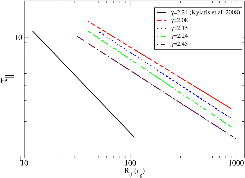
Figure 7: Relationship between the optical depth, $\tau_{\parallel}$, and the width at the base of the jet, $R_{0}$, for the models that reproduce the observations. Four different sets of models (discontinuous lines) are shown. Each set (line) was created by varying $\tau_{\parallel}$ and $R_{0}$, while $\gamma$ remained fixed at the value indicated. For comparison, we also show (continuous line) the relation between optical depth and jet width in the absence of an acceleration region from (from Kylafis et al., 2008).

6 Conclusions

We have performed an X-ray timing and spectral analysis of twelve outbursts of eight black-hole binaries and found that the slope of the hard spectral continuum correlates with the time lag of hard photons with respect to softer photons. As the source evolves in the hard state the spectral continuum becomes softer and the time lag increases. The correlation is particularly strong and significant during the rise of the outburst. Remarkably this correlation appears to be a universal property of BHBs. We demonstrate that Comptonization of low-energy photons by very energetic electrons in a jet can explain these results. The different cutoff energy is explained by invoking different jet velocities.

References

- Akritas & Bershady (1996) Akritas, M. G. & Bershady, M. A. 1996, ApJ, 470, 706
- Altamirano & Méndez (2015) Altamirano, D. & Méndez, M. 2015, MNRAS, 449, 4027
- Arévalo & Uttley (2006) Arévalo, P. & Uttley, P. 2006, MNRAS, 367, 801
- Armas Padilla et al. (2013) Armas Padilla, M., Degenaar, N., Russell, D. M., & Wijnands, R. 2013, MNRAS, 428, 3083
- Band & Grindlay (1986) Band, D. L. & Grindlay, J. E. 1986, ApJ, 311, 595
- Belloni & Hasinger (1990) Belloni, T. & Hasinger, G. 1990, A&A, 227, L33
- Belloni et al. (2011) Belloni, T. M., Motta, S. E., & Muñoz-Darias, T. 2011, Bulletin of the Astronomical Society of India, 39, 409
- Böck et al. (2011) Böck, M., Grinberg, V., Pottschmidt, K., et al. 2011, A&A, 533, A8
- Cassatella et al. (2012) Cassatella, P., Uttley, P., Wilms, J., & Poutanen, J. 2012, MNRAS, 422, 2407
- Chen et al. (1997) Chen, W., Shrader, C. R., & Livio, M. 1997, ApJ, 491, 312
- Contopoulos & Kazanas (1998) Contopoulos, I. & Kazanas, D. 1998, ApJ, 508, 859
- Coppi (1999) Coppi, P. S. 1999, in Astronomical Society of the Pacific Conference Series, Vol. 161, High Energy Processes in Accreting Black Holes, ed. J. Poutanen & R. Svensson, 375
- Crary et al. (1998) Crary, D. J., Finger, M. H., Kouveliotou, C., et al. 1998, ApJ, 493, L71
- Di Matteo & Psaltis (1999) Di Matteo, T. & Psaltis, D. 1999, ApJ, 526, L101
- Dunn et al. (2010) Dunn, R. J. H., Fender, R. P., Körding, E. G., Belloni, T., & Cabanac, C. 2010, MNRAS, 403, 61
- Esin et al. (1997) Esin, A. A., McClintock, J. E., & Narayan, R. 1997, ApJ, 489, 865
- Fender & Belloni (2012) Fender, R. & Belloni, T. 2012, Science, 337, 540
- Fender et al. (2004) Fender, R. P., Belloni, T. M., & Gallo, E. 2004, MNRAS, 355, 1105
- Fender et al. (2009) Fender, R. P., Homan, J., & Belloni, T. M. 2009, MNRAS, 396, 1370
- Garain et al. (2012) Garain, S. K., Ghosh, H., & Chakrabarti, S. K. 2012, ApJ, 758, 114
- Georganopoulos et al. (2002) Georganopoulos, M., Aharonian, F. A., & Kirk, J. G. 2002, A&A, 388, L25
- Ghosh et al. (2011) Ghosh, H., Garain, S. K., Giri, K., & Chakrabarti, S. K. 2011, MNRAS, 416, 959
- Giannios (2005) Giannios, D. 2005, A&A, 437, 1007, "Paper III"
- Giannios et al. (2004) Giannios, D., Kylafis, N. D., & Psaltis, D. 2004, A&A, 425, 163, "Paper II"
- Grinberg et al. (2013) Grinberg, V., Hell, N., Pottschmidt, K., et al. 2013, A&A, 554, A88
- Grinberg et al. (2014) Grinberg, V., Pottschmidt, K., Böck, M., et al. 2014, A&A, 565, A1
- Hanke et al. (2009) Hanke, M., Wilms, J., Nowak, M. A., et al. 2009, ApJ, 690, 330
- Hua & Titarchuk (1995) Hua, X.-M. & Titarchuk, L. 1995, ApJ, 449, 188
- Jahoda et al. (2006) Jahoda, K., Markwardt, C. B., Radeva, Y., et al. 2006, ApJS, 163, 401
- Kalamkar et al. (2015) Kalamkar, M., Reynolds, M. T., van der Klis, M., Altamirano, D., & Miller, J. M. 2015, ApJ, 802, 23
- Kalemci (2002) Kalemci, E. 2002, PhD thesis, University of California, San Diego
- Kalemci et al. (2005) Kalemci, E., Tomsick, J. A., Buxton, M. M., et al. 2005, ApJ, 622, 508
- Kalemci et al. (2003) Kalemci, E., Tomsick, J. A., Rothschild, R. E., et al. 2003, ApJ, 586, 419
- Kotov et al. (2001) Kotov, O., Churazov, E., & Gilfanov, M. 2001, MNRAS, 327, 799
- Kylafis & Belloni (2015a) Kylafis, N. D. & Belloni, T. M. 2015a, in Astrophysics and Space Science Library, Vol. 414, The Formation and Disruption of Black Hole Jets, ed. I. Contopoulos, D. Gabuzda, & N. Kylafis, 245
- Kylafis & Belloni (2015b) Kylafis, N. D. & Belloni, T. M. 2015b, A&A, 574, A133
- Kylafis et al. (2012) Kylafis, N. D., Contopoulos, I., Kazanas, D., & Christodoulou, D. M. 2012, A&A, 538, A5
- Kylafis et al. (2008) Kylafis, N. D., Papadakis, I. E., Reig, P., Giannios, D., & Pooley, G. G. 2008, A&A, 489, 481, "Paper IV"
- Levine et al. (1996) Levine, A. M., Bradt, H., Cui, W., et al. 1996, ApJ, 469, L33
- Markoff et al. (2005) Markoff, S., Nowak, M. A., & Wilms, J. 2005, ApJ, 635, 1203
- McNamara et al. (2009) McNamara, A. L., Kuncic, Z., & Wu, K. 2009, MNRAS, 395, 1507
- Migliari & Fender (2006) Migliari, S. & Fender, R. P. 2006, MNRAS, 366, 79
- Migliari et al. (2007) Migliari, S., Miller-Jones, J. C. A., Fender, R. P., et al. 2007, ApJ, 671, 706
- Miller-Jones et al. (2010) Miller-Jones, J. C. A., Sivakoff, G. R., Altamirano, D., et al. 2010, ApJ, 716, L109
- Miyamoto et al. (1991) Miyamoto, S., Kimura, K., Kitamoto, S., Dotani, T., & Ebisawa, K. 1991, ApJ, 383, 784
- Motta et al. (2009) Motta, S., Belloni, T., & Homan, J. 2009, MNRAS, 400, 1603
- Muñoz-Darias et al. (2011) Muñoz-Darias, T., Motta, S., & Belloni, T. M. 2011, MNRAS, 410, 679
- Narayan & Yi (1994) Narayan, R. & Yi, I. 1994, ApJ, 428, L13
- Nowak et al. (2011) Nowak, M. A., Hanke, M., Trowbridge, S. N., et al. 2011, ApJ, 728, 13
- Nowak et al. (1999) Nowak, M. A., Vaughan, B. A., Wilms, J., Dove, J. B., & Begelman, M. C. 1999, ApJ, 510, 874
- Nowak et al. (2002) Nowak, M. A., Wilms, J., & Dove, J. B. 2002, MNRAS, 332, 856
- Pottschmidt et al. (2003) Pottschmidt, K., Wilms, J., Nowak, M. A., et al. 2003, A&A, 407, 1039
- Reig & Kylafis (2015) Reig, P. & Kylafis, N. D. 2015, A&A, 584, A109
- Reig et al. (2003) Reig, P., Kylafis, N. D., & Giannios, D. 2003, A&A, 403, L15, "Paper I"
- Reig et al. (2013) Reig, P., Papadakis, I. E., Sobolewska, M. A., & Malzac, J. 2013, MNRAS, 435, 3395
- Rothschild et al. (1998) Rothschild, R. E., Blanco, P. R., Gruber, D. E., et al. 1998, ApJ, 496, 538
- Shakura & Sunyaev (1973) Shakura, N. I. & Sunyaev, R. A. 1973, A&A, 24, 337
- Shaposhnikov & Titarchuk (2009) Shaposhnikov, N. & Titarchuk, L. 2009, ApJ, 699, 453
- Shidatsu et al. (2014) Shidatsu, M., Ueda, Y., Yamada, S., et al. 2014, ApJ, 789, 100
- Sobolewska et al. (2011) Sobolewska, M. A., Papadakis, I. E., Done, C., & Malzac, J. 2011, MNRAS, 417, 280
- Stiele et al. (2013) Stiele, H., Belloni, T. M., Kalemci, E., & Motta, S. 2013, MNRAS, 429, 2655
- Sunyaev & Titarchuk (1980) Sunyaev, R. A. & Titarchuk, L. G. 1980, A&A, 86, 121
- Tomsick et al. (2001) Tomsick, J. A., Corbel, S., & Kaaret, P. 2001, ApJ, 563, 229
- Tomsick et al. (2004) Tomsick, J. A., Kalemci, E., & Kaaret, P. 2004, ApJ, 601, 439
- Wilms et al. (2006) Wilms, J., Nowak, M. A., Pottschmidt, K., Pooley, G. G., & Fritz, S. 2006, A&A, 447, 245
- Wu & Gu (2008) Wu, Q. & Gu, M. 2008, ApJ, 682, 212
- Zdziarski (1998) Zdziarski, A. A. 1998, MNRAS, 296, L51