Edge sampling using network local information

Abstract.

Edge sampling is an important topic in network analysis. It provides a natural way to reduce network size while retaining desired features of the original network. Sampling methods that only use local information are common in practice as they do not require access to the entire network and can be parallelized easily. Despite promising empirical performances, most of these methods are derived from heuristic considerations and therefore still lack theoretical justification. To address this issue, we study in this paper a simple edge sampling scheme that uses network local information. We show that when local connectivity is sufficiently strong, the sampled network satisfies a strong spectral property. We quantify the strength of local connectivity by a global parameter and relate it to more common network statistics such as the clustering coefficient and network curvature. Based on this result, we also provide sufficient conditions under which random networks and hypergraphs can be sampled efficiently.

1. Introduction

Network analysis has become an important area in many research domains. It provides a natural way to model and analyze data with a complex interdependence among entities. A network typically consists of a set of nodes representing the entities of interest and a set of edges between nodes encoding the relations between the nodes. For example, in a social network such as Facebook or Twitter, nodes are users and there is an edge between two users if they are friends. Studying the structure of a network provides valuable information about how entities interact and may help predict the formation of different groups [18, 15].

As real-world networks are often very large, it is difficult and often impossible to store or even get access to the entire data set. It is therefore desirable to preprocess the data to reduce the network size before performing any analysis. A natural method for this task is graph sparsification, a well-known edge sampling method in network literature [8, 49, 48]. For a network of $n$ nodes, one samples edges independently with probabilities proportional to their effective resistances, i.e. the electrical resistances between the same nodes in the resistor network obtained from the original network by replacing edges with resistors of unit conductance [16]. It has been shown that sampling and storing $O(n\log n)$ weighted edges is sufficient for approximately preserving the important topological structure of the original network [48]. Specifically, for an undirected network $G=(V,E)$ with the set of nodes $V=\{1,2,...,n\}$ and the set of edges $E\subseteq V\times V$, let $A$ be the adjacency matrix with $A_{ij}=1$ if $(i,j)\in E$ and $A_{ij}=0$ otherwise. Let $L_{G}=D-A$ be the Laplacian, where $D$ is the diagonal matrix with node degrees $d_{i}=\sum_{j\in V}A_{ij}$ on the diagonal, and define the Laplacian $L_{H}$ for the weighted network $H$ output by graph sparsification in a similar way. Then $H$ satisfies the following inequality for every $x\in\mathbb{R}^{n}$, known as the strong spectral property:

$$(1-\varepsilon)x^{\mathsf{T}}L_{G}x\leq x^{\mathsf{T}}L_{H}x\leq(1+\varepsilon)x^{\mathsf{T}}L_{G}x.$$ (1.1)

Although this method has a strong theoretical guarantee, a serious drawback it suffers from, especially when applied to very large networks, is that it requires access to the entire network for computing effective resistances of all edges. Also, the computation involves a complicated linear system solver of Spielman and Teng, not easy to implement in practice. Although some improvements of [48] have been proposed, they still rely on complicated linear system solvers [24, 23].

To avoid this problem, several fast and simple edge sampling methods have been developed with more emphasis on preserving certain network features such as the number of connected components, network diameter, homophily, node centrality measures or community structure [35]. One of the simplest sampling methods is uniform sampling, which samples edges independently and uniformly at random [43, 30]. More adaptive methods leverage the strong local connectivity of networks that is widely observed in practice: the network neighborhoods of most of the nodes are surprisingly dense [53, 50]. They sample edges according to certain edge scores that can be calculated locally without access to the entire network such as the Jaccard similarity score [44], the number of triangles [20] or the number of quadrangles containing the edges under consideration [37]; see also [20] for methods based on other local measures. Although these methods have been empirically shown to perform well and can be parallelized easily, to our best knowledge, there is still no theoretical guarantee for their performances. It is also unclear if other features of networks (besides the targeting features considered) are preserved.

In an attempt to understand the theoretical properties of these methods, in this paper we study a fast and simple edge sampling scheme similar to methods that use Jaccard similarity or number of triangles [44, 20]. Specifically, for an undirected network $G=(V,E)$, we sample each edge $(i,j)\in E$ with probability inversely proportional to the number of common neighbors of $i$ and $j$ (i.e. those nodes connected to both $i$ and $j$). The numbers of common neighbors have been used in network literature, for example in the context of community detection [42] and network embedding [40].

We observe that when the numbers of common neighbors are sufficiently large compared to node degrees, our sampling method satisfies the same strong spectral property (1.1) that the graph sparsification does, while avoiding the complicated calculation of effective resistances. This result also provides theoretical evidence supporting edge sampling methods based on local statistics [44, 37, 20]. Qualitatively, as the number of common neighbors increases, the network local connectivity gets stronger and our sampling method becomes more similar to graph sparsification using effective resistances. In contrast, as the numbers of common neighbors decrease, the method becomes more similar to uniform sampling. We quantify the strength of the network local connectivity by the following parameter

$$\alpha=\frac{1}{n}\sum_{(i,j)\in E}\frac{2}{t_{ij}+2},$$ (1.2)

where $t_{ij}$ denotes the number of common neighbors of node $i$ and node $j$. As we will show, $\alpha$ is closely related to other well-known and similar in nature statistics such as the clustering coefficient [53] and network curvature [5]; see Section 3 for the definition. More importantly, it determines the sample size (the number of sampled edges) needed for the strong spectral property to hold.

1.1. Our contributions

We make the following contributions in this paper. First, in Section 2 we propose a simple sampling method by leveraging the strong local connectivity that has been often observed for real-world networks and show that it satisfies the strong spectral property (1.1) if we sample $O(\alpha n\log n)$ edges, where $\alpha$ is defined by (1.2). As a direct consequence, we show that uniform sampling with replacement also satisfies (1.1) if the sample size is sufficiently large; the exact value is given by (2.4). This requirement can be relaxed if a hybrid sampling method that combines both uniform sampling and sampling according to the number of common neighbors is used. Second, we provide lower and upper bounds on $\alpha$ for general networks in terms of the clustering coefficient and network curvature (Section 3). Since $\alpha$ directly determines the sample size required for the strong spectral property, these bounds provide useful information about when our sampling method can be used efficiently. They also show a connection with other sampling methods that use different local statistics [44, 37, 20] for which the theory developed in this paper may potentially be applied. Third, in Section 4 we provide an upper bound on $\alpha$ for the general inhomogeneous Erdős-Rényi random graph model [11]. Since this model is very popular in network literature, the bound provides a rich class of examples for which our sampling method can be used for reducing the network size. We discuss in Section 5 another natural class of examples, the hypergraphs, for which our method can be found useful. Lastly, in Section 7 we show that $\alpha$ is small for many real-world networks and perform a thorough numerical study to evaluate our sampling method.

1.2. Related work

The simplest sampling method is bond percolation, which independently selects edges with a fixed probability $\varepsilon$ [3, 34, 10]. If $\varepsilon$ is sufficiently large so that $\Omega(n\log n)$ edges are selected then with high probability the adjacency matrix of the sparsified network concentrates around $\varepsilon A$ by a standard matrix concentration result [38]. The advantage of this method is that it is fast and only requires the total number of edges in the network as a global input parameter. However, it satisfies a much weaker property than the strong spectral property [49]. A closely related method is uniform sampling, for which [43] shows that (1.1) holds with high probability, but only for smooth vectors $x$.

In semi-streaming setting, [8] and [17] show that local network structure can be used to design sampling methods that approximately preserve all cuts of the original network; here, the cut of a set of nodes is the number of edges between that set and its complement in $V$. However, this property is strictly weaker than the strong spectral property that our method satisfies [24].

2. Edge sampling using common neighbors

For an undirected network $G=(V,E)$ and $(i,j)\in E$, let $t_{ij}$ be the number of common neighbors of $i$ and $j$. For simplicity of presentation, we first discuss the case when $t_{ij}$ are known for all edges. In practice, they can be either exactly calculated in a parallel manner or approximated by neighbor sampling; see Section 6 for a more detailed discussion. To form a sparsifier $H$, we sample $m$ edges of $G$ independently according to a multinomial distribution with probabilities

$$p_{ij}=\frac{\frac{2}{t_{ij}+2}}{\sum_{(i,j)\in E}\frac{2}{t_{ij}+2}}.$$ (2.1)

If an edge $(i,j)\in E$ is selected $k\geq 1$ times then we add it to $H$ and assign the weight $k(mp_{ij})^{-1}$ to it.

Note that $2/(t_{ij}+2)$ is the effective resistance of the edge between $i$ and $j$ in a subgraph of $G$ consisting of the edge $(i,j)$ and $t_{ij}$ paths of length two between $i$ and $j$. It is therefore an upper bound of the effective resistance of the edge between $i$ and $j$ in $G$; for a detailed explanation, see the proof of Theorem 2.2 in Appendix A.

The following theorem shows that our sampling method satisfies the strong spectral property.

Theorem 2.1 (Sampling method using $t_{ij}$).

Consider an undirected and connected network $G=(V,E)$. Let $\varepsilon\in(0,1)$ and $\alpha$ be the parameter of $G$ defined by (1.2). Form a weighted network $H$ by sampling $8\alpha n\log n/\varepsilon^{2}$ edges of $G$ as described above. Then $H$ satisfies the strong spectral property (1.1) with probability at least $1-1/n$.

Parameter $\alpha$ measures the average strength of network local connectivity. To better understand $\alpha$, consider a special case when $d_{i}=d$ for all vertices $i$ and $t_{ij}=t$ for all edges $(i,j)\in E$. Then $\alpha\approx 2|E|/(nt)=d/t$, where here and after we use $|\mathcal{M}|$ to denote the number of elements of the set $\mathcal{M}$. Thus, if $(i,j)\in E$ then the number of common neighbors of $i$ and $j$ is approximately $d/\alpha$. In other words, $i$ and $j$ share a fraction of $1/\alpha$ of their neighbors.

When the local connectivity is strong, i.e. $\alpha=O(1)$, Theorem 2.1 shows that we can approximately preserve the network topology if we locally sample and retain $O(n\log n)$ edges. In contrast, if the local connectivity is weak (for example when $t_{ij}=O(1)$) then $p_{ij}$ are of the same order, resulting in a sampling scheme similar to uniform sampling. Table 2 shows the value of $\alpha$ and the clustering coefficient (see Section 3.1 for the definition) for several well-known real-world networks. Note that while these networks are relatively sparse, the values of $\alpha$ are quite small, which suggests that real-world networks have strong local connectivity.

The above sampling method requires access to the number of common neighbors $t_{ij}$ for all pairs of incident nodes. If $t_{ij}$ are readily available, which is the case for some social networks such as Facebook, then the computational complexity of this sampling method is linear in the total number of edges $|E|$. When $t_{ij}$ are not available, we can calculate them in parallel fashion or estimate them by neighbor sampling; see Section 6 for more detail. The following theorem shows that the strong spectral property still holds if we use estimates of $t_{ij}$ and increase the sample size by a factor depending on the accuracy of the estimates.

Theorem 2.2 (Sampling method using estimates of $t_{ij}$).

Consider an undirected and connected network $G=(V,E)$ and let $\hat{t}_{ij}$ be nonnegative estimates of $t_{ij}$ such that

$$\hat{t}_{ij}+2\leq C(t_{ij}+2)$$ (2.2)

for all edges $(i,j)\in E$ and some constant $C$. Let $\varepsilon\in(0,1)$ and denote

$$\hat{\alpha}=\frac{1}{n}\sum_{(i,j)\in E_{G}}\frac{2}{\hat{t}_{ij}+2}.$$ (2.3)

Form a weighted graph $H$ by sampling $8C\hat{\alpha}n\log n/\varepsilon^{2}$ edges of $G$ as described in Theorem 2.1 but using $\hat{t}_{ij}$ instead of $t_{ij}$. Then $H$ satisfies the spectral property (1.1) with probability at least $1-1/n$.

The proof of Theorem 2.2 depends crucially on condition (2.2). It implies that $2/(t_{ij}+2)\leq 2C/(\hat{t}_{ij}+2)$ and consequently the effective resistance of the edge $(i,j)$ is bounded by $2C/(\hat{t}_{ij}+2)$. This observation allows us to express the Laplacian of the sparsified network as a sum of independent matrices with spectral norms bounded by $C\hat{\alpha}n$ up to a scaling matrix factor. A standard matrix concentration result is then used to show the strong spectral property; see the proof in Appendix A for more detail. Note that Theorem 2.1 follows directly from Theorem 2.2 by setting $\hat{t}_{ij}=t_{ij}$ and $C=1$.

One may wonder how many edges must be sampled so that the uniform sampling (which samples edges with probabilities $p_{ij}=1/|E|$) satisfies the spectral property (1.1). The uniform sampling is obtained by setting $\hat{t}_{ij}=t$ for all edges of $G$ in Theorem 2.2. The constant $C$ can be taken to be

$$C=\frac{t+2}{\min_{(i,j)\in E}t_{ij}+2}\quad\text{and}\quad\hat{\alpha}=\frac{2|E|}{n(T+2)}.$$

Therefore by Theorem 2.2, the uniform sampling satisfies (1.1) with high probability if the sample size is

$$m=\frac{16\varepsilon^{-2}|E|\log n}{\min_{(i,j)\in E}t_{ij}+2}.$$ (2.4)

If $\min_{(i,j)\in E}t_{ij}$ is of order $|E|/n$, i.e. numbers of common neighbors are at least a constant fraction of the average degree, then $m=O(n\log n)$.

In general, the sample size requirement (2.4) is optimal up to the logarithm and constant factors. That is, (1.1) needs not hold if $m=o(|E|/(\min_{(i,j)\in E}t_{ij}+2))$. To see this, consider an example of a graph $G$ consisting of a complete graph of $n-1$ nodes and a node $i$ of degree $k=o(n)$. Then $\min_{(i,j)\in E}t_{ij}=k-1$. If $m=o(|E|/(k+1))$ and edges of $G$ are sampled uniformly then the probability that no edges incident to $i$ is selected is

$$\left(1-\frac{k}{|E|}\right)^{m}=\left(1-\frac{k}{|E|}\right)^{\frac{|E|}{k}\cdot\frac{mk}{|E|}}\approx\exp\left(-\frac{mk}{|E|}\right)\approx 1.$$

That is, with probability close to one, $i$ is an isolated node in the (weighted) sparsified graph. Therefore the degree of $i$ cannot be approximately preserved, which implies that the spectral property (1.1) does not hold.

For graphs with small value of $\min_{(i,j)\in E}t_{ij}$, the sample size $m$ in (2.4) for the uniform sampling scheme may get as large as the total number of edges $|E|$, which defies the purpose of graph sparsification. By choosing $\hat{t}_{ij}=t$ only if $t_{ij}>t$ for some large threshold $t$ and $\hat{t}_{ij}=t_{ij}$ if $t_{ij}\leq t$, we obtain a hybrid of uniform sampling and sampling using common neighbors that may require smaller sample size than (2.4). Indeed, in Theorem 2.2, we can choose $C=1$ and

$$\hat{\alpha}=\frac{1}{n}\sum_{(i,j)\in E:t_{ij}\leq t}\frac{2}{t_{ij}+2}+\frac{1}{n}\sum_{(i,j)\in E:t_{ij}>t}\frac{2}{t+2}\leq\alpha+\frac{2|E|}{n(t+2)}.$$

The required sample size for the hybrid method to obtain the spectral property (1.1) with high probability is then

$$8\varepsilon^{-2}C\hat{\alpha}n\log n\leq 8\varepsilon^{-2}\left(\alpha+\frac{2|E|}{n(t+2)}\right)n\log n=8\varepsilon^{-2}\alpha n\log n+\frac{16|E|\log n}{\varepsilon^{2}(t+2)},$$

which is smaller than the sample size in (2.4) if $\alpha n=o(|E|/(\min_{(i,j)\in E}t_{ij}+2))$ and $\min_{(i,j)\in E}t_{ij}=o(t)$. This hybrid method illustrates an interesting application of Theorem 2.2 and may also be useful when uniform sampling is desirable, for example for controlling the variance of the sparsified graph.

3. Bounding parameter $\alpha$

In this section we draw the connection between the parameter $\alpha$ and two of the most common network statistics, the clustering coefficient [53] and the network curvature [5].

3.1. Lower bound

It has been observed that for many real-world networks, the neighborhoods of most of the nodes are surprisingly dense [53, 50]. This reflects the belief that incident nodes exhibit the transitivity property: if $i$ and $j$ are connected and $j$ and $k$ are connected then it is likely that $i$ and $k$ are also connected. One way to measure the transitivity is via the clustering coefficient [53]. For an undirected network $G=(V,E)$, the local clustering coefficient of node $i\in V$ is defined as the ratio between the number of triangles containing $i$ and the maximum number of triangles it can form with incident nodes

$$c_{i}=\frac{|\{(j,k)\in E:(i,j)\in E,(i,k)\in E\}|}{d_{i}(d_{i}-1)/2}.$$

The clustering coefficient of a network $G$ is the average of all local clustering coefficients

$$c=\frac{1}{n}\sum_{i=1}^{n}c_{i}.$$

The following theorem provides a lower bound on parameter $\alpha$ in terms of the clustering coefficient $c$ and node degrees $d_{i}$. It shows that if node degrees are large and $c$ is small then $\alpha$ is large and therefore a large sample size is required for our method to obtain the spectral property (1.1). On the other hand, Table 2 suggests that $\alpha$ is small when $c$ is large. Since the clustering coefficient is a very popular statistic and has been calculated for most of available real-world networks, the connection to the clustering coefficient provides valuable information about $\alpha$ before the sampling procedure is performed.

Theorem 3.1 (Lower bound on $\alpha$).

For any undirected and connected network we have

$$\alpha\geq\frac{1}{4c+\frac{2}{n}\sum_{i=1}^{n}\frac{1}{d_{i}}}.$$ (3.1)

According to Theorem 3.1, if $c\gtrsim 1/n\sum_{i\in V}1/d_{i}$ then $\alpha$ satisfies $\alpha\gtrsim 1/c$ (for two sequences $a_{n}$ and $b_{n}$, we write $a_{n}\gtrsim b_{n}$ if $a_{n}\geq Cb_{n}$ for some constant $C$ and sufficiently large $n$). The geometric random graph model described in Corollary 4.2 below provides examples for which the upper bound $\alpha\lesssim 1/c$ also holds; for more detail, see the discussion following Corollary 4.2. In addition, Table 2 gives examples of real networks for which $\alpha$ and $1/c$ are of similar order.

There exist graphs for which the two sides of (3.1) are of different orders. For example, let $G=K_{n}\cup E_{n}$ be the union of a complete graph $K_{n}$ of size $n$ and an Erdős-Rényi random graph $E_{n}$, also of size $n$, for which edges are formed independently between each pair of nodes with probability $d/n$; we connect $K_{n}$ and $E_{n}$ by an arbitrary edge to make $G$ a connected graph. If $\sqrt{n}\lesssim d=o(n)$ then an easy calculation shows that with high probability, the left hand-side of (3.1) is of order $n/d$ while the right hand-side is bounded.

3.2. Upper bound

Another measure of network transitivity that has recently attracted much attention is the network curvature [5, 22, 31, 9]. In this section we recall the definition of network curvature and show that if it is bounded from below by some constant $\kappa_{0}>0$ then $\alpha\leq 1/\kappa_{0}$.

Denote by $d(i,j)$ the length of a shortest path connecting nodes $i$ and $j$. For each node $i$, consider a uniform measure $m_{i}$ with support being the set $N_{i}$ of neighbors of $i$:

$$m_{i}(k)=\left\{\begin{array}[]{ll}\frac{1}{d_{i}},&\hbox{if }k\in N_{i}\\ 0,&\hbox{otherwise.}\end{array}\right.$$

The optimal transportation distance between $m_{i}$ and $m_{j}$ is defined as follows:

$$W_{1}(m_{i},m_{j})=\inf_{\xi\in\Pi(m_{i},m_{j})}\sum_{(k,k^{\prime})\in V\times V}d(k,k^{\prime})\xi(k,k^{\prime}),$$

where $\Pi(m_{i},m_{j})$ is the set of all probability measures on $V\times V$ with marginals $m_{i}$ and $m_{j}$. Intuitively, $\xi(k,k^{\prime})$ represents the mass transported from $k$ to $k^{\prime}$, and $W_{1}(m_{i},m_{j})$ is the optimal cost for moving a unit mass distributed evenly among neighbors of $i$ to neighbors of $j$. With this notion of distance between probability measures on $G$, the curvature $\kappa$ defined for every pair of nodes $i$ and $j$ is

$$\kappa(i,j)=1-\frac{W_{1}(m_{i},m_{j})}{d(i,j)}.$$

To illustrate, in Figure 1 we show the Zachary’s karate club network [55] together with the information of its curvatures for incident nodes. In particular, edges with negative curvatures are in blue, positive curvatures – in red and zero curvatures – in black; widths of edges are proportional to magnitudes of curvatures.

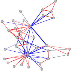
Figure 1. Zachary’s karate club network [55]. Edges with negative curvatures are in blue, positive curvatures – in red and zero curvatures – in black; widths of the edges are proportional to the magnitudes of their curvatures.

We say $\kappa\geq\kappa_{0}$ for some constant $\kappa_{0}$ if $\kappa(i,j)\geq\kappa_{0}$ for every pair of nodes $i$ and $j$. If $\kappa\geq\kappa_{0}$ then by definition $W_{1}(m_{i},m_{j})\leq(1-\kappa_{0})d(i,j)$ for all $(i,j)\in V\times V$. In particular, if $i$ and $j$ are connected then $W_{1}(m_{i},m_{j})\leq 1-\kappa_{0}$. Note that if $G$ is a connected graph then the inverse is also true: If $W_{1}(m_{i},m_{j})\leq 1-\kappa_{0}$ holds for all pairs of connected nodes $i$ and $j$ then $W_{1}(m_{i},m_{j})\leq(1-\kappa_{0})d(i,j)$ holds for all $(i,j)\in V\times V$ by a triangle inequality.

This notion of curvature is closely related to the simple random walk on a network. If $\kappa\geq\kappa_{0}>0$ then [39] shows that the spectral gap between the two largest eigenvalues of the transition matrix $D^{-1}A$ is bounded from below by $\kappa_{0}$ (see also [5] for an improvement of the bound). Thus, the curvature of a graph controls how fast a simple random walk on that network mixes.

The following theorem provides a simple upper bound on $\alpha$ in terms of the curvature.

Theorem 3.2 (Upper bound on $\alpha$).

Let $G$ be an undirected and connected network. Assume there exist constants $\kappa_{0}>0$ and $C>0$ such that $\kappa(i,j)\geq\kappa_{0}$ for all but at most $Cn$ edges of $G$. Then $\alpha\leq 1/\kappa_{0}+C$.

4. Random networks

In this section we provide a high probability bound on $\alpha$ for inhomogeneous Erdős-Rényi random networks [11] satisfying some mild conditions. As a corollary, we give an example of a geometric random network model for which $\alpha$ is bounded.

Theorem 4.1 (Inhomogeneous Erdős-Rényi networks).

Consider a random graph with adjacency matrix $A$ such that the upper diagonal elements of $A$ are independent Bernoulli random variables. Denote $P=\operatorname{\mathbb{E}}A$ and $\Delta=\max_{i}\sum_{j=1}^{n}P_{ij}$. Assume that there exists a sufficiently large constant $C$ such that

$$\Delta\geq C\log n\qquad\text{and}\qquad\Delta\cdot\left[1+\max_{i,j}\left(P^{2}\right)_{ij}\right]\leq\frac{1}{C\log n}\sum_{i<j}P_{ij}.$$ (4.1)

Then with probability at least $1-1/n$,

$$\alpha\leq\frac{1}{n}\sum_{i<j}\frac{10P_{ij}}{\operatorname{\mathbb{E}}t_{ij}+2}.$$ (4.2)

In particular, if the right-hand side of (4.2) is bounded then $\alpha$ is also bounded.

The first inequality of (4.1) requires that the maximal expected node degree grow at least as $\log n$; this is a natural condition because otherwise the network would already be sparse and no sampling would be needed. The second inequality of (4.1) is a condition on the maximal expected degree $\Delta$, the maximal expected number of common neighbors $\max_{ij}(P^{2})_{ij}$ and the expected number of edges $1/2\sum_{i<j}P_{ij}$. If all nodes in the graph are of similar expected degree then $\sum_{i<j}P_{ij}\approx n\Delta$. Therefore, using the crude bound $(P^{2})_{ij}\leq\Delta$, the second inequality of (4.1) is satisfied if $\Delta$ is at most of order $n/\log n$.

By Jensen’s inequality and the independence between $A_{ij}$ and $t_{ij}$, we have

$$\operatorname{\mathbb{E}}\alpha=\frac{1}{n}\sum_{i<j}\operatorname{\mathbb{E}}\frac{2A_{ij}}{t_{ij}+2}=\frac{1}{n}\sum_{i<j}\operatorname{\mathbb{E}}\frac{2P_{ij}}{t_{ij}+2}\geq\frac{1}{n}\sum_{i<j}\frac{2P_{ij}}{\operatorname{\mathbb{E}}t_{ij}+2}.$$

It then follows from (4.2) that $\alpha\leq 5\operatorname{\mathbb{E}}\alpha$ with probability at least $1-1/n$, while naively applying Markov’s inequality gives the same inequality with probability at least $4/5$. Note, however, that the upper bound of (4.2) is much easier to calculate than $\operatorname{\mathbb{E}}\alpha$.

As a direct consequence of Theorem 4.1, the following corollary shows that $\alpha$ is bounded for a simple geometric random network model.

Corollary 4.2 (Geometric random networks).

Let $X=\{x_{1},x_{2},...,x_{n}\}\subseteq K$ be a set of points in a bounded set $K\subseteq\mathbb{R}^{d}$ with unit volume. For each pair of nodes $(i,j)$, let

$$P_{ij}=\begin{cases}\delta,&\text{if }\|x_{i}-x_{j}\|\leq r_{n},\\ 0,&\text{otherwise}.\end{cases}$$

Denote by $n_{i}$ the number of points of $X$ of distance at most $R_{n}$ from $x_{i}$; similarly, denote by $n_{ij}$ the number of points of $X$ of distance at most $R_{n}$ from $x_{i}$ and $x_{j}$. Assume that there exists a constant $C=C(d,K)$ depending only on $d$ and $K$ such that for every node $i$ and every node $j$ with $\|x_{j}-x_{i}\|\leq r_{n}$,

$$C^{-1}nr_{n}^{d}\leq n_{i},n_{ij}\leq Cnr_{n}^{d}\quad\text{and}\quad C^{2}\delta^{-1}\log n\leq nr_{n}^{d}\leq\frac{n}{4C^{3}\delta^{2}\log n}.$$ (4.3)

Then $\alpha\leq 5C^{2}/\delta$ with probability at least $1-1/n$.

The first condition of (4.3) holds with high probability if $x_{1},...,x_{n}$ are independently drawn from a uniform distribution on $K$. Indeed, for every node $i$, $n_{i}/n$ is approximately the volume of the ball of radius $r_{n}$ and center $x_{i}$, which is proportional to $r_{n}^{d}$ up to a constant depending on $d$ and $K$; a similar argument holds for $n_{ij}$ with $\|x_{j}-x_{i}\|\leq r_{n}$. The second condition of (4.3) requires that the average degree of the graph be roughly between $\log n$ and $n/\log n$. If these conditions are satisfied then $\alpha$ is bounded with high probability.

Theorem 3.1 shows that $\alpha\gtrsim 1/c$ if the clustering coefficient $c$ is at least of the same order as $1/n\sum_{i\in V}1/d_{i}$. Corollary 4.2 provides examples for which the reverse bound also holds. Indeed, since $\alpha\lesssim 1/\delta$ with high probability by Corollary 4.2, the bound $\alpha\lesssim 1/c$ holds if $c\gtrsim\delta$ with high probability. To see why that is the case, for every node $i$ let $N_{i}$ be the set of all neighbors of $i$. Then conditioned on $N_{i}$, the probability that two neighbors of $i$ are connected is at most $\delta$. Therefore the number of triangles containing $i$ is stochastically bounded by a sum of $d_{i}(d_{i}-1)/2$ independent Bernoulli random variables with success probability $\delta$. Using a standard concentration result and union bounds, we see that the local clustering coefficients satisfy $c_{i}\lesssim\delta$ for all $i$ with high probability. Since $c$ is the average of $c_{i}$, this implies $c\gtrsim\delta$ with high probability.

5. Sampling hypergraphs

Strong local connectivity of a network is often caused by the fact that each node belongs to one or several tightly connected small groups [19]. To simplify the analysis, we assume that within each small group, all nodes are connected. Under this assumption, a network can be modeled by a hypergraph $\mathcal{G}=(V,\mathcal{E})$ which consists of a set of nodes $V$ and a set of hyperedges $\mathcal{E}$ where each hyperedge is a subset of $V$. In this section we derive a condition under which a hypergraph can be sampled and reduced to a weighted network. This provides another example for which our sampling scheme works well and may be useful in practice as a computational acceleration technique.

The Laplacian previously defined for networks can be naturally extended to hypergraphs through clique expansion [41, 2]. For a hypergraph $\mathcal{G}=(V,\mathcal{E})$, the evaluation of the Laplacian $L_{\mathcal{G}}$ at a vector $x$ is defined by

$$L_{\mathcal{G}}(x)=\sum_{e\in\mathcal{E}}\sum_{i,j\in e}(x_{i}-x_{j})^{2}.$$

If we view $x$ as a function from $V$ to $\mathbb{R}$ then $L_{\mathcal{G}}(x)$ measures the smoothness of $x$ and it occurs naturally in many problems of estimating smooth functions [47, 7, 21, 25, 30, 27].

Let $G=(V,E,W)$ be a weighted network such that $(i,j)\in E$ if and only if both $i$ and $j$ belong to at least one hyperedge of $\mathcal{G}$, and $W$ denotes the weight matrix with entries $W_{ij}$ being the number of hyperedges that both $i$ and $j$ belong to. It is easy to see that $L_{\mathcal{G}}(x)=x^{\mathsf{T}}L_{G}x$ for every $x$, where $L_{G}$ is the Laplacian of the weighted network $G$ defined by

$$x^{\mathsf{T}}L_{G}x=\sum_{(i,j)\in E}W_{ij}(x_{i}-x_{j})^{2}.$$

Thus, if we are mainly interested in the smoothness of functions determined by $\mathcal{G}$ then we can replace $\mathcal{G}$ with $G$. We call $G$ the weighted network induced by $\mathcal{G}$.

To form a sparsifier $H=(V,E_{H},W_{H})$ of $G$, we sample with replacement $m$ edges of $G$ with probability

$$\mathcal{P}_{ij}=\frac{\tilde{t}_{ij}^{-1}}{\sum_{(i,j)\in E}\tilde{t}_{ij}^{-1}},\quad\text{where}\quad\tilde{t}_{ij}=\sum_{e\in\mathcal{E}:\{i,j\}\in e}|e|.$$

If an edge $(i,j)\in E$ is selected $k\geq 1$ times then we add $(i,j)$ to $E_{H}$ and assign the weight $k(m\mathcal{P}_{ij})^{-1}$ to it. Similar to the parameter $\alpha$ for unweighted graphs, let

$$\tilde{\alpha}=\frac{1}{n}\sum_{(i,j)\in E}\tilde{t}_{ij}^{-1}.$$

Lemma 5.1 (Upper bound on $\tilde{\alpha}$).

Let $\mathcal{G}=(V,\mathcal{E})$ be a hypergraph. If each node of $\mathcal{G}$ belongs to at most $d$ hyperedges then $\tilde{\alpha}\leq d/2$.

Without further assumptions on $\mathcal{G}$, the bound $\tilde{\alpha}\leq d/2$ is nearly optimal. To see this, consider the following example. Let $k>0$ be an integer, $n=k^{2}$ and $V_{1},...,V_{k}$ be a partition of $V=\{1,...,n\}$ such that each $V_{i}$ contains exactly $k$ elements $V_{i1},...,V_{ik}$. For each $1\leq i\leq k$, let $\sigma_{i}$ be a permutation of $\{1,2,...,k\}$ given by $\sigma_{i}(j)=i+j$ (mode $k$). Define the set of hyperedges of $\mathcal{G}$ as a collection of subsets of the form

$$\left\{V_{1j},V_{2\sigma_{i}(j)},...,V_{k\sigma_{i}^{k-1}(j)}\right\},\quad 1\leq i,j\leq k.$$

It is easy to see that every node of $\mathcal{G}$ is contained in exactly $d=k$ hyperedges and every pair of nodes of $\mathcal{G}$ is contained in at most one hyperedge. A simple calculation shows that $\tilde{\alpha}=(d-1)/2$.

The following theorem shows that the sparsified network obtained from a hypergraph satisfies the strong spectral property.

Theorem 5.2 (Sampling hypergraphs).

Let $\mathcal{G}=(V,\mathcal{E})$ be a hypergraph and $G=(V,E,W)$ be the weighted network induced by $\mathcal{G}$. Let $\varepsilon\in(0,1)$ and assume that each node of $\mathcal{G}$ belongs to at most $d$ hyperedges of $\mathcal{G}$. Form a weighted graph $H$ by sampling $4dn\log n/\varepsilon^{2}$ edges of $G$ as described above. Then $H$ satisfies the strong spectral property (1.1) with probability at least $1-1/n$.

6. Calculating the number of common neighbors

In this section we discuss the problem of calculating $t_{ij}$ (either exactly or approximately), especially when the network is too large to be stored in a single computer. Once $t_{ij}$ are all computed, the sampling method can be performed easily by sampling edges according to $t_{ij}$ and aggregating over all sampled edges.

6.1. Exact calculation

The number of common neighbors $t_{ij}$ can be calculated efficiently by using an MPI-based distributed memory parallel algorithm in [4], with very little modification. The algorithm first carefully partitions the graph into smaller overlapping subgraphs and stores them separately in local machines. A sequential algorithm then finds all triangles in every subgraph and counts the number of common neighbors for every connected pair of nodes in that subgraph. Since an edge of the original graph may belong to different overlapping subgraphs, the counts from all local machines are then aggregated before the final result is output. The authors of [4] show that their algorithm scales almost linearly in the number of local machines and can handle very large graphs with billions of edges.

6.2. Estimation

Depending on the strength of the local connectivity of a graph, the computational complexity of our sampling method can be further improved by approximating $t_{ij}$ instead of calculating them exactly. In this section we describe a simple method for estimating $t_{ij}$ by sampling the neighbors of either $i$ or $j$. A similar idea has been used in minwise hashing, a popular technique for efficiently estimating the Jaccard similarity between two sets [13, 14, 6, 44, 45, 46]. Although the method described here is sequential in nature, we can easily turn it into a parallel algorithm by adapting the method of [4] discussed in Section 6.1.

For each pair of connected nodes $(i,j)$, denote by $N_{i}$ the set of neighbors of $i$ and by $N_{j}$ the set of neighbors of $j$. The asymmetric Jaccard similarity between $N_{i}$ and $N_{j}$ is defined by

$$\theta_{ij}=\frac{|N_{i}\cap N_{j}|}{\min\{|N_{i}|,|N_{j}|\}}=\frac{t_{ij}}{\min\{d_{i},d_{j}\}}.$$

Fix a sample size $k\geq 1$ and assume that $d_{i}\leq d_{j}$. If $k\geq d_{i}$ then simply counting the number of neighbors of $i$ that are also neighbors of $j$ gives us exactly $t_{ij}$. If $k<d_{i}$, let $Z_{1},...,Z_{k}$ be $k$ random neighbors of $i$ drawn independently and uniformly from $N_{i}$. We estimate $t_{ij}$ by

$$\hat{t}_{ij}=\frac{d_{i}}{k}\sum_{\ell=1}^{k}{\bf 1}(Z_{\ell}\in N_{j}),$$

where ${\bf 1}(Z_{\ell}\in N_{j})$ is the indicator of the event $Z_{\ell}\in N_{j}$. It is easy to see that $\hat{t}_{ij}$ is an unbiased estimate of $t_{ij}$ because ${\bf 1}(Z_{\ell}\in N_{j})$, $1\leq\ell\leq k$, are Bernoulli random variables with success probability $\theta_{ij}$.

In order to apply Theorem 2.2, condition (2.2) must be satisfied for all edges $(i,j)\in E_{G}$. For those edges such that $\theta_{ij}\geq\varepsilon$ for some constant $\varepsilon$, we will show that (2.2) holds with high probability if $k$ is chosen to be of order $\log n$. For those edges with $\theta_{ij}=o(1)$, $\hat{t}_{ij}$ may not satisfy (2.2) if $k=O(\log n)$, therefore we calculate $t_{ij}$ directly. We use $\frac{1}{k}\sum_{\ell=1}^{k}{\bf 1}(Z_{\ell}\in N_{j})$ to check whether $\theta_{ij}$ is sufficiently large. The estimation procedure is summarized in the following algorithm.

Algorithm 1.

(Estimating number of common neighbors) Choose $\varepsilon\in(0,1)$ and $k\geq 1$. For each edge $(i,j$), let $i$ be the node with $d_{i}\leq d_{j}$. If $d_{i}\leq k$, calculate $t_{ij}$ directly by counting the number of elements of $N_{i}\cap N_{j}$. If $d_{i}>k$, sample $k$ neighbors $Z_{1},...,Z_{k}$ of $i$ independently and uniformly from $N_{i}$, calculate $\hat{\theta}_{ij}=\frac{1}{k}\sum_{\ell=1}^{k}{\bf 1}(Z_{\ell}\in N_{j})$ and proceed as follows:

• If $\hat{\theta}_{ij}<\varepsilon$, calculate $t_{ij}$ directly by counting the number of elements of $N_{i}\cap N_{j}$.

• If $\hat{\theta}_{ij}\geq\varepsilon$, estimate $t_{ij}$ by $\hat{t}_{ij}=d_{i}\hat{\theta}_{ij}$.

The following theorem provides the spectral guarantee (1.1) for the sparsified network when Algorithm 1 is used.

Theorem 6.1 (Sampling method using $\hat{t}_{ij}$).

Let $\varepsilon\in(0,1)$, $k=100\log n/\varepsilon$ and estimate the numbers of common neighbors using Algorithm 1. Form a weighted graph $H$ by sampling $24{\alpha}n\log n/\varepsilon^{2}$ edges of $G$ according to Theorem 2.2. Then with probability at least $1-1/n$, $H$ satisfies the spectral property (1.1) and the computational complexity of estimating the number of common neighbors is at most

$$\sum_{(i,j)\in E_{G}:\theta_{ij}\leq\varepsilon/2}\min\{d_{i},d_{j}\}+100\varepsilon^{-1}|E_{G}|\log n.$$ (6.1)

The complexity of estimating the number of common neighbors in Theorem 6.1 is nearly linear in the number of edges $|E_{G}|$ (up to the $\log n$ factor) and depends on the local structure of the network via the first term of (6.1). If the local connectivity of $G$ is sufficiently strong so that $\theta_{ij}\geq\varepsilon/2$ for all edges then the first term disappears. However, for networks with very weak local connectivity, such as Erdős-Rényi random networks, the first term of (6.1) may be as large as $d\cdot|E_{G}|$, where $d$ is the average node degree. In that case, it is not clear if the computational complexity of the (sequential) estimation algorithm can be substantially improved; we leave this problem for future study.

Section 7.2 shows the performance of the proposed sampling method using both exact and estimated numbers of common neighbors.

7. Numerical study

7.1. Parameter $\alpha$

According to Theorem 2.1, $\alpha$ directly controls the accuracy of our sampling method. In this section we show that $\alpha$ is relatively small for many simulated and real-world networks.

7.1.1. Simulated networks

We consider geometric inhomogeneous random networks (GIRG) generated from a latent space model which has been shown to exhibit several properties of real-world networks such as the strong transitivity and the power law distribution of node degrees [12]. To model the power law, each node $i$ is assigned a weight $w_{i}=\delta\cdot(n/i)^{1/(\beta-1)}$, where $\delta>0$ and $2\leq\beta\leq 3$ are parameters. The latent positions $x_{i}$ are drawn uniformly at random from an $r$-dimensional torus $\mathbb{T}^{r}=\mathbb{R}^{r}/\mathbb{Z}^{r}$ equipped with the distance

$$d(u,v)=\max_{1\leq k\leq r}\min\{|u_{k}-v_{k}|,1-|u_{k}-v_{k}|\}.$$

For a parameter $\gamma>1$ and $w=\sum_{i=1}^{n}w_{i}$, an edge is independently drawn between each pair of nodes $i,j$ with probability

$$p_{ij}=\min\left\{\frac{1}{\|x_{i}-x_{j}\|^{\gamma r}}\Big{(}\frac{w_{i}w_{j}}{w}\Big{)}^{\gamma},1\right\}.$$

We report in Table 1 the value of $\alpha$, the clustering coefficient and the average node degree (averaged over 20 replications) of networks generated from GIRG with parameter $\delta=\gamma=2$, $r=3$, $\beta=2.5$ and $n=100,500,1000,2000,4000$. Table 1 shows that while the network size and average node degree increase, the value of $\alpha$ increases mildly from 1.84 to 2.65 and the clustering coefficient decreases from 0.59 to 0.52.

Network size	100	500	1000	2000	4000
Parameter $\alpha$	1.84	2.34	2.49	2.59	2.65
Clustering coefficient	0.59	0.53	0.52	0.52	0.52
Average degree	27.64	36.42	38.89	40.89	42.57

Table 1. Statistics of networks generated from the GIRG with $\delta=\gamma=2$, $r=3$ and $\beta=2.5$, averaged over 20 replications.

7.1.2. Real-world networks

We further report in Table 2 the value of $\alpha$, the clustering coefficient and the average degree of several well-known real-world networks: karate club network [55], dolphins network [32], political blogs network [1], Facebook ego network [33], Astrophysics collaboration network [28], Enron email network [26], Twitter Social circles [54], Google+ social circles [54], DBLP collaboration network [54] and LiveJournal social network [54]. Again, we observe that while the network size and average node degree vary, $\alpha$ and the clustering coefficient are very stable, with the value of $\alpha$ between 1.40 and 4.38 and the value of the clustering coefficient between 0.26 and 0.63, respectively.

Data	$n$	Average degree	$c$	$\alpha$
Karate club	$34$	$4.59$	$0.57$	$1.46$
Dolphins	$62$	$5.13$	$0.26$	$1.65$
Political blogs	$1490$	$22.44$	$0.32$	$3.04$
Facebook ego	$4039$	$43.69$	$0.61$	$1.96$
Astrophysics collaboration	$18771$	$21.10$	$0.63$	$1.96$
Enron email	$36692$	$10.02$	$0.50$	$1.59$
Twitter	$81306$	$33.02$	$0.57$	$2.33$
Google+	$107614$	$227.45$	$0.49$	$4.38$
DBLP collaboration	$317080$	$6.62$	$0.63$	$1.40$
LiveJournal	$3997962$	$17.35$	$0.28$	$3.65$

Table 2. Statistics of some real-world networks.

7.2. Accuracy of network sampling

In this section, we compare the performance of our sampling method that uses the number of common neighbors (CN), the uniform sampling (UN) and a version of CN that uses $\hat{t}_{ij}$ defined in (6.2) to approximate the number of common neighbors (CNA). We use these methods to sparsify networks, both simulated and real-world, and then measure the accuracy of the resulting sparsified networks by comparing their Laplacians with those of the original networks. Motivated naturally by the strong spectral property (1.1), for a connected network $G$ and its sparsification $H$, we report the following relative error

$$\text{Relative error}=\max_{x:L_{G}x\neq 0}\frac{x^{\mathsf{T}}(L_{H}-L_{G})x}{x^{\mathsf{T}}L_{G}x}=\|L_{G}^{-1/2}(L_{H}-L_{G})L_{G}^{-1/2}\|,$$ (7.1)

where $L_{G}^{-1/2}$ is the square root of the Moore–Penrose pseudo-inverse $L_{G}^{-1}$ of $L_{G}$. This error reflects the accuracy of $H$ in preserving the structure of $G$. Since calculating the relative error involves inverting the Laplacian, we consider in this section only networks of relatively small sizes.

7.2.1. Simulated networks

We first analyze the performance of CN, CNA and UN on random networks generated from the latent space stochastic block model [36], which has been shown to capture important characteristics of real-world networks. Specifically, we assume that nodes are partitioned into three disjoint groups or communities, and conditioning on the community labels, subsetworks corresponding to the communities follow the GIRG model defined in Section 7.1 with $\gamma=\delta=1$, $\beta=3$ and $r=10$. Edges between nodes in different communities are independently drawn with the same probability adjusted so that the ratio of the expected numbers of edges between communities and within communities equals $\rho\in\{0.01,0.1\}$, which measures the strength of the community structure.

For each $\rho\in\{0.01,0.1\}$, we consider three settings corresponding to different community size ratios $(1/20,9/20,1/2)$, $(1/10,2/5,1/2)$ and $(1/3,1/3,1/3)$. In the first two settings, network communities are of very different sizes, while in the last setting, all communities are of the same size $n/3$. The networks generated in these settings are relatively dense for the sampling purpose, with expected degree ranging approximately from 300 to 500. We vary the sample size $m$ by setting $m=\tau n$, where $\tau$ is the sample size factor taking values from 10 to 210. To approximate the number of common neighbors for CNA, we sample $k=50$ neighbors using Algorithm 1.

Figure 2 shows the relative error averaged over 10 repetitions of CN, CNA and UN in three settings and different values of $\rho$. We observe that as the sample size $m$ increases, all methods perform better, with CN slightly better than CNA, and both methods are more accurate than UN when the communities are of different sizes and especially when $\rho=0.01$. This is because when $\rho$ is small and one community is of much smaller size than the others, UN focuses on sampling edges within large communities, mostly ignoring edges between communities and within the smallest community. In contrast, CN and CNA sample more edges within the smallest community and between communities because they have fewer common neighbors, resulting in better estimates of the Laplacian. However, when all communities are of the same size, UN tends to perform better than CN and CNA. This is perhaps because no part of any balanced and dense network needs to be sampled much more frequently than others, and UN often performs well in this case [43]. However, real networks are usually far from balanced, and UN may be much less accurate than CN and CNA when they are applied to these networks, as we will show next.

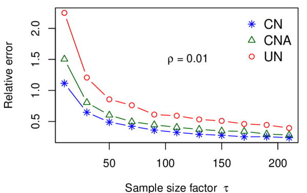
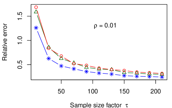
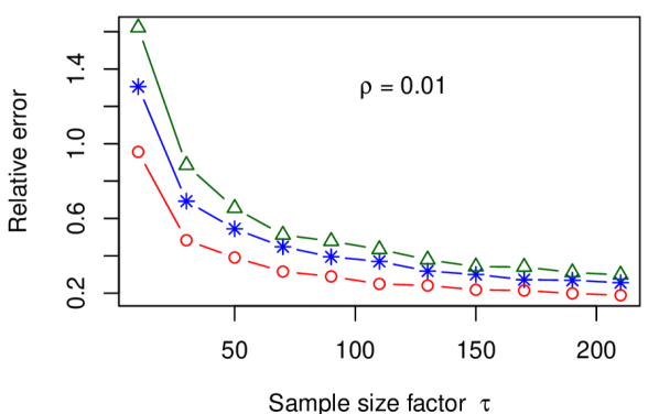
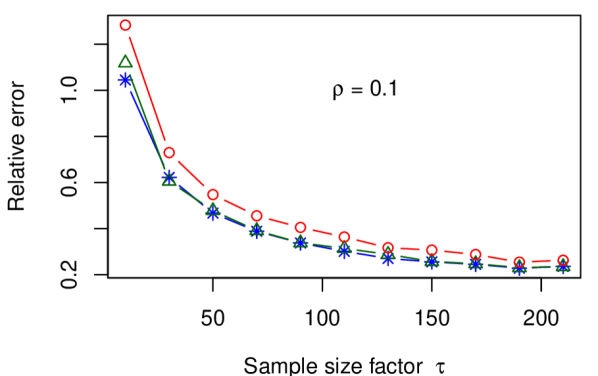
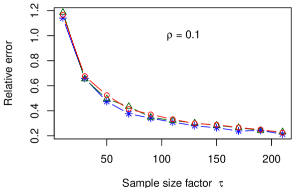
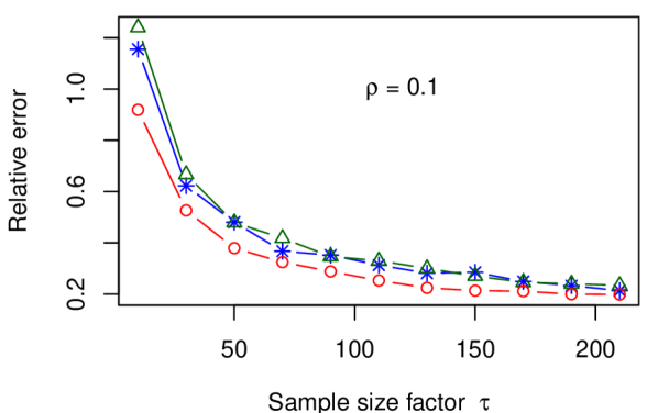
Figure 2. Accuracy of different sampling methods on random networks.

7.2.2. Real-world networks

We further compare the performance of CN, CNA and UN on the political blogs network [1] and the Facebook ego network [33], the two largest networks in Table 2 for which inverting the Laplacian can be done reasonably fast. (Note that the matrix inversion is only needed for calculating the relative error in (7.1) while our proposed methods can easily handle all networks in Table 2.) Similar to the analysis in the previous section, we vary the sample size $m$ by setting $m=\tau n$ with $\tau\in[10,50]$. To approximate the number of common neighbors for CNA, we sample $k=20$ neighbors according to Algorithm 1. Figure 3 shows that as $\tau$ increases, all three methods perform better, with CN slightly better than CNA, both having much smaller errors than UN.

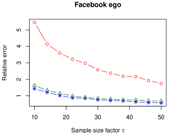
Figure 3. Accuracy of different sampling methods on real networks.

Note that the performance gap between UN and the proposed methods is much more visible on the real networks than on simulated networks shown in the previous section. This is probably due to the significant difference between the distributions of the number of common neighbors of simulated and real networks. As shown in Figure 4, most of the edges of the simulated networks have very large numbers of common neighbors, and for such nodes, the uniform sampling performs well (this is partially explained in the discussion following Theorem 2.2). In contrast, edges of the real networks considered here have relatively smaller numbers of common neighbors, resulting in the much worse performance of the uniform sampling. The numerical results on real networks show that sampling using the number of common neighbors may be very useful in practice.

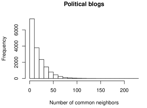
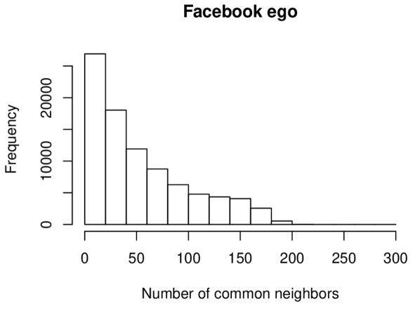
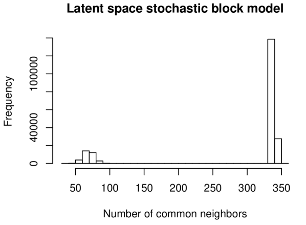
Figure 4. Distributions of the number of common neighbors for the political blogs network, the Facebook ego network and a network generated from a latent space stochastic block model described in Section 7.2.1 with community size ratios $(1/3,1/3,1/3)$ and $\rho=0.1$.

8. Discussion

In this paper we study an edge sampling algorithm that uses only the number of common neighbors. This simple statistic provides an easy way to measure the strength of network local connectivity through parameter $\alpha$, which directly controls the accuracy of the sampling method. However, in practice we often have access to not only the numbers of common neighbors but also neighborhood networks around edges. In that case, we should use the information from these local networks, provided that it is available or easily computed, because it contains more structural information of the network than just the numbers of common neighbors. Measuring the strength of local connectivity through local networks is more challenging and we leave it for future work.

Appendix A Proofs of results in Section 2

Theorem 2.1 directly follows from Theorem 2.2 with $\hat{t}_{ij}=t_{ij}$ for all edges $(i,j)\in E_{G}$ and $C=1$. To prove Theorem 2.2, we use the following result about the concentration of the sum of random matrices [51].

Theorem A.1 (Concentration of sum of matrices).

Let $Y_{1},...,Y_{m}$ be independent $n\times n$ random positive semidefinite matrices such that $\|Y_{k}\|\leq M$ for all $1\leq k\leq m$. Let $S_{m}=\sum_{k=1}^{m}Y_{k}$ and $E=\sum_{k=1}^{m}\|\operatorname{\mathbb{E}}Y_{k}\|$. Then for every $\varepsilon\in(0,1)$ we have

$$\mathbb{P}\left\{\|S_{m}-\operatorname{\mathbb{E}}S_{m}\|>\varepsilon E\rule{0.0pt}{8.53581pt}\right\}\leq n\cdot\exp\left(\frac{-\varepsilon^{2}E}{4M}\right).$$

Proof of Theorem 2.2.

Let $X$ be a random matrix such that

$$X=\frac{1}{p_{ij}}(e_{i}-e_{j})(e_{i}-e_{j})^{\mathsf{T}}\quad\text{with probability }\ \hat{p}_{ij},$$

where $(i,j)\in E_{G}$, $\{e_{i},1\leq i\leq n\}$ are standard basis vectors (the $i$th entry of $e_{i}$ is one and all other entries are zero), and

$$\hat{p}_{ij}=\frac{\frac{2}{\hat{t}_{ij}+2}}{\sum_{(i,j)\in E_{G}}\frac{2}{\hat{t}_{ij}+2}}.$$ (A.1)

Then

$$\operatorname{\mathbb{E}}X=\sum_{(i,j)\in E_{G}}\hat{p}_{ij}\times\frac{1}{\hat{p}_{ij}}(e_{i}-e_{j})(e_{i}-e_{j})^{\mathsf{T}}=L_{G}.$$ (A.2)

Let $X_{k}$ be $m$ independent copies of $X$. By the sampling scheme we have

$$L_{H}=\frac{1}{m}\sum_{k=1}^{m}X_{k},\quad\operatorname{\mathbb{E}}L_{H}=L_{G}.$$

Denote by $L_{G}^{-1}$ the Moore-Penrose pseudoinverse of $L_{G}$ and by $L_{G}^{-1/2}$ the squared root of $L_{G}^{-1}$. Note that the kernel of the map $L_{G}$ is a one-dimensional vector space spanned by the all-one vector ${\bf 1}$ and it is contained in the kernel of $L_{H}$. Therefore the strong spectral property (1.1) is equivalent to

$$(1-\varepsilon)I_{\bf 1}\preceq\frac{1}{m}\sum_{k=1}^{m}L_{G}^{-1/2}X_{k}L_{G}^{-1/2}\preceq(1+\varepsilon)I_{\bf 1},$$ (A.3)

where $I_{\bf 1}=I-(1/n){\bf 1}{\bf 1}^{\mathsf{T}}$ is the identity map on the $(n-1)$-dimensional subspace orthogonal to the all-one vector ${\bf 1}$. Here, we write $U\preceq V$ if $V-U$ is positive semidefinite.

To prove (A.3), we apply Theorem A.1 to $Y_{k}:=L_{G}^{-1/2}X_{k}L_{G}^{-1/2}$. Since $X_{k}\succeq 0$ and $\operatorname{\mathbb{E}}X_{k}=L_{G}$ by (A.2), it follows that $Y_{k}\succeq 0$ and $\|\operatorname{\mathbb{E}}Y_{k}\|=\|I_{\bf 1}\|=1$. To bound $\|Y_{k}\|$, note that $Y_{k}$ takes one of the following matrix values

$$\frac{1}{\hat{p}_{ij}}\left(L_{G}^{-1/2}(e_{i}-e_{j})\right)\left(L_{G}^{-1/2}(e_{i}-e_{j})\right)^{\mathsf{T}},\quad(i,j)\in E_{G}.$$

By (A.1) and (2.3) we have $1/\hat{p}_{ij}=n\hat{\alpha}(\hat{t}_{ij}+2)/2$. Therefore

$$\|Y_{k}\|\leq\max_{(i,j)\in E_{G}}\frac{n\hat{\alpha}(\hat{t}_{ij}+2)}{2}\cdot(e_{i}-e_{j})^{\mathsf{T}}L_{G}^{-1}(e_{i}-e_{j}).$$ (A.4)

Note that $(e_{i}-e_{j})^{\mathsf{T}}L_{G}^{-1}(e_{i}-e_{j})$ is the effective resistance of the edge between $i$ and $j$ [16]. We claim that it is upper bounded by $2/(t_{ij}+2)$. To show that, let $N_{ij}$ be the set of common neighbors of $i$ and $j$. Denote by $G_{ij}=(V_{ij},E_{ij})$ the subgraph of $G$ such that

$$V_{ij}=\{i,j\}\cup N_{ij},\qquad E_{ij}=\{(i,j),(i,k),(j,k):k\in N_{ij}\}.$$

Thus, $G_{ij}$ consists of an edge and $t_{ij}$ paths of length two between $i$ and $j$. It is easy to see that the effective resistance $(e_{i}-e_{j})^{\mathsf{T}}L^{-1}_{G_{ij}}(e_{i}-e_{j})$ of the edge between $i$ and $j$ in $G_{ij}$ is $2/(t_{ij}+2)$. Indeed, let $x=L^{-1}_{G_{ij}}(e_{i}-e_{j})$. Then $L_{G_{ij}}x=e_{i}-e_{j}$ and by comparing the $i$-th and $j$-th components of $L_{G_{ij}}x$ and $e_{i}-e_{j}$, we have

$$(t_{ij}+1)x_{i}-x_{j}-\sum_{k\in N_{ij}}x_{k}=1,\qquad x_{i}-(t_{ij}+1)x_{j}+\sum_{k\in N_{ij}}x_{k}=1.$$

Adding these equalities, we obtain that the effective resistance of the edge between $i$ and $j$ in $G_{ij}$ is $(e_{i}-e_{j})^{\mathsf{T}}x=x_{i}-x_{j}=2/(t_{ij}+2)$. Since $G_{ij}$ is a subgraph of $G$ and adding edges does not increase the effective resistance (see e.g. Corollary 9.13 in [29]), it follows that

$$(e_{i}-e_{j})^{\mathsf{T}}L_{G}^{-1}(e_{i}-e_{j})\leq(e_{i}-e_{j})^{\mathsf{T}}L^{-1}_{G_{ij}}(e_{i}-e_{j})=\frac{2}{t_{ij}+2}.$$

Together with (A.4) this implies $\|Y_{k}\|\leq n\hat{\alpha}(\hat{t}_{ij}+2)/(t_{ij}+2)\leq n\hat{\alpha}C$. Therefore by Theorem A.1 we have

$$\mathbb{P}\left\{\left\|\frac{1}{m}\sum_{k=1}^{m}Y_{k}-I_{{\bf 1}}\right\|>\varepsilon\rule{0.0pt}{8.53581pt}\right\}\leq n\cdot\exp\left(\frac{-\varepsilon^{2}m}{4C\hat{\alpha}n}\right).$$

Inequality (A.3) then follows by choosing $m=8C\hat{\alpha}n\log n/\varepsilon^{2}$. ∎

Appendix B Proofs of results in Section 3

Proof of Theorem 3.2.

Let $(i,j)$ be an edge of $G$ such that $\kappa(i,j)\geq\kappa_{0}$ or equivalently $W_{1}(m_{i},m_{j})\leq 1-\kappa_{0}$. Recall that

$$W_{1}(m_{i},m_{j})=\inf_{\xi\in\Pi(m_{i},m_{j})}\sum_{(k,k^{\prime})\in V\times V}d(k,k^{\prime})\xi(k,k^{\prime}),$$

where $\Pi(m_{i},m_{j})$ is the set of all probability measures on $V\times V$ with marginals $m_{i}$ and $m_{j}$. For every $\xi\in\Pi(m_{i},m_{j})$,

$$\xi(k,k)\leq\min\left\{\sum_{k^{\prime}\in V}\xi(k^{\prime},k),\sum_{k^{\prime}\in V}\xi(k,k^{\prime})\right\}=\min\{m_{j}(k),m_{i}(k)\}.$$

Since $m_{i}$ and $m_{j}$ are uniform measures with supports being the sets of neighbors of $i$ and $j$, respectively, if $k$ is not a common neighbor of $i$ and $j$ then $\min\{m_{j}(k),m_{i}(k)\}=0$; when $k$ is one of the $t_{ij}$ common neighbors of $i$ and $j$ then $\min\{m_{j}(k),m_{i}(k)\}=\min\{1/d_{i},1/d_{j}\}$. Therefore

$$\sum_{k\in V}\xi(k,k)\leq t_{ij}\cdot\min\{1/d_{i},1/d_{j}\},$$

which implies

$$\sum_{(k,k^{\prime})\in V\times V}d(k,k^{\prime})\xi(k,k^{\prime}) = \sum_{k\neq k^{\prime}}d(k,k^{\prime})\xi(k,k^{\prime})$$

$$\geq \sum_{k\neq k^{\prime}}\xi(k,k^{\prime})$$

$$= 1-\sum_{k\in V}\xi(k,k)$$

$$\geq 1-t_{ij}\cdot\min\{1/d_{i},1/d_{j}\}.$$

Taking the infimum over all $\xi\in\Pi(m_{i},m_{j})$, we have

$$1-\kappa_{0}\geq W_{1}(m_{i},m_{j})\geq 1-t_{ij}\cdot\min\{1/d_{i},1/d_{j}\},$$

or $t_{ij}\geq\kappa_{0}/\min\{1/d_{i},1/d_{j}\}$. Denote by $\mathcal{E}$ the set of all edges of $G$ such that $\kappa(i,j)\geq\kappa_{0}$ and by $\mathcal{E}^{c}$ its complement. Since $|\mathcal{E}^{c}|\leq Cn$ by assumption,

$$\alpha = \frac{1}{n}\sum_{(i,j)\in\mathcal{E}}\frac{2}{2+t_{ij}}+\frac{1}{n}\sum_{(i,j)\in\mathcal{E}^{c}}\frac{2}{2+t_{ij}}$$

$$\leq \frac{2}{\kappa_{0}n}\sum_{(i,j)\in\mathcal{E}}\min\{1/d_{i},1/d_{j}\}+C$$

$$\leq \frac{1}{\kappa_{0}n}\sum_{i\in V}\sum_{j\in N_{i}}\min\{1/d_{i},1/d_{j}\}+C$$

$$\leq \frac{1}{\kappa_{0}}+C.$$

For the last inequality, we use the fact that $\sum_{j\in N_{i}}\min\{1/d_{i},1/d_{j}\}\leq 1$. ∎

For proving Theorem 3.1, we need the following lemma.

Lemma B.1.

For positive numbers $x_{1},x_{2},...,x_{k}$ the following inequality holds

$$\left(x_{1}+x_{2}+\cdots+x_{k}\right)\left(\frac{1}{x_{1}}+\frac{1}{x_{2}}+\cdots+\frac{1}{x_{k}}\right)\geq k^{2}.$$

The two sides are equal if and only if $x_{1}=x_{2}=\cdots=x_{n}$.

Proof of Lemma B.1.

Using the inequality of arithmetic and geometric means, we have

$$x_{1}+x_{2}+\cdots+x_{k}\geq k(x_{1}x_{2}\cdots x_{k})^{1/k},\quad\frac{1}{x_{1}}+\frac{1}{x_{2}}+\cdots+\frac{1}{x_{k}}\geq k(x_{1}x_{2}\cdots x_{k})^{-1/k}.$$

Lemma B.1 follows directly from these inequalities. ∎

Proof of Theorem 3.1.

For each node $i$, denote by $N_{i}$ and $t_{i}$ the set of neighbors of $i$ and the number of triangles that contain $i$, respectively. Using Lemma B.1, we have

$$\sum_{j\in N_{i}}\frac{2}{t_{ij}+2}\geq\frac{2|N_{i}|^{2}}{\sum_{j\in N_{i}}(t_{ij}+2)}=\frac{d_{i}^{2}}{t_{i}+d_{i}}\geq\frac{1}{2c_{i}+\frac{1}{d_{i}}}.$$

Summing over all nodes $i$ and applying Lemma B.1 again, we obtain

$$\sum_{(i,j)\in E}\frac{4}{t_{ij}+2}\geq\sum_{i\in V}\frac{1}{2c_{i}+\frac{1}{d_{i}}}\geq\frac{|V|^{2}}{\sum_{i\in V}\left(2c_{i}+\frac{1}{d_{i}}\right)}=\frac{n}{2c+\frac{1}{n}\sum_{i\in V}\frac{1}{d_{i}}}.$$

The proof is complete by dividing both sides of this inequality by $2n$. ∎

Appendix C Proofs of results in Section 4

Proof of Theorem 4.1.

We rewrite $S:=n\alpha$ as follows:

$$S=\sum_{(i,j)\in E_{G}}\frac{2}{t_{ij}+2}=\sum_{i<j}\frac{2A_{ij}}{t_{ij}+2}=:\sum_{i<j}Y_{ij}.$$

The proof consists of two parts: showing that $S\leq 2\operatorname{\mathbb{E}}S$ with high probability and upper bounding $\operatorname{\mathbb{E}}S$. For the first part, note that $S$ is a sum of $n(n-1)/2$ weakly depdendent random variables $Y_{ij}=2A_{ij}/(t_{ij}+2)$, where $Y_{ij}$ and $Y_{i^{\prime}j^{\prime}}$ are independent if $i^{\prime}\neq i$ and $j^{\prime}\neq j$. To deal with the dependence among $Y_{ij}$, we will use the moment method (see for example [52]).

For notational simplicity, we denote $\gamma=\{i,j\}$ as a set of two elements $i,j$ and write $S=\sum_{\gamma}Y_{\gamma}$. With the new notation, $Y_{\gamma}$ and $Y_{\gamma^{\prime}}$ are independent if $\gamma\cap\gamma^{\prime}=\emptyset$. For a positive integer $k$, let

$$M_{k}=\sum_{(\gamma_{1},...,\gamma_{k})}\prod_{i=1}^{k}Y_{\gamma_{i}},$$

where the sum is over all $k$-tuples $(\gamma_{1},...,\gamma_{k})$ such that $\gamma_{i}\cap\gamma_{j}=\emptyset$ if $i\neq j$. Since $Y_{\gamma_{1}},Y_{\gamma_{2}},...,Y_{\gamma_{k}}$ are independent by construction,

$$\operatorname{\mathbb{E}}M_{k}=\sum_{(\gamma_{1},...,\gamma_{k})}\prod_{i=1}^{k}\operatorname{\mathbb{E}}Y_{\gamma_{i}}\leq\left(\sum_{\gamma}\operatorname{\mathbb{E}}Y_{\gamma}\right)^{k}=\left(\operatorname{\mathbb{E}}S\right)^{k}.$$ (C.1)

Denote by $\mathcal{E}$ the event that $S>2\operatorname{\mathbb{E}}S$. When $\mathcal{E}$ occurs,

$$M_{k+1} = \sum_{(\gamma_{1},...,\gamma_{k})}\prod_{i=1}^{k}Y_{\gamma_{i}}\left(\sum_{\gamma}Y_{\gamma}-\sum_{\gamma\cap\gamma_{i}\neq\emptyset\text{ for some }1\leq i\leq k}Y_{\gamma}\right)$$

$$\geq \sum_{(\gamma_{1},...,\gamma_{k})}\prod_{i=1}^{k}Y_{\gamma_{i}}\left(2\operatorname{\mathbb{E}}S-\sum_{\gamma\cap\gamma_{i}\neq\emptyset\text{ for some }1\leq i\leq k}Y_{\gamma}\right).$$

For each $(\gamma_{1},...,\gamma_{k})$ we have

$$\sum_{\gamma\cap\gamma_{i}\neq\emptyset\text{ for some }1\leq i\leq k}Y_{\gamma}\leq\sum_{i=1}^{k}\sum_{\gamma\cap\gamma_{i}\neq\emptyset}Y_{\gamma}\leq k\cdot\max_{\gamma^{\prime}}\sum_{\gamma\cap\gamma^{\prime}\neq\emptyset}Y_{\gamma}.$$

Let $Z=\max_{i}\sum_{j=1}^{n}A_{ij}$ be the maximal node degree. Since $Y_{\gamma}\leq A_{\gamma}$,

$$\max_{\gamma^{\prime}}\sum_{\gamma\cap\gamma^{\prime}\neq\emptyset}Y_{\gamma}\leq\max_{\gamma^{\prime}}\sum_{\gamma\cap\gamma^{\prime}\neq\emptyset}A_{\gamma}\leq 2Z.$$

Therefore if $\mathcal{E}$ occurs then

$$M_{k+1}\geq\sum_{(\gamma_{1},...,\gamma_{k})}\prod_{i=1}^{k}Y_{\gamma_{i}}\left(2\operatorname{\mathbb{E}}S-2kZ\right)=M_{k}\left(2\operatorname{\mathbb{E}}S-2kZ\right).$$ (C.2)

We now show that $2\operatorname{\mathbb{E}}S-2kZ\geq(3/2)\cdot\operatorname{\mathbb{E}}S>0$ with high probability for $k=O(\log n)$, so the above inequality can be applied repeatedly to obtain a desired lower bound for $M_{k}$. Since upper diagonal elements of $A$ are independent, by Jensen’s inequality we have

$$\operatorname{\mathbb{E}}S=\sum_{i<j}P_{ij}\cdot\operatorname{\mathbb{E}}\left[\frac{2}{t_{ij}+2}\right]\geq\sum_{i<j}\frac{2P_{ij}}{\operatorname{\mathbb{E}}t_{ij}+2}\geq\ \frac{2}{\max_{i,j}\operatorname{\mathbb{E}}t_{ij}+2}\cdot\sum_{i<j}P_{ij}.$$

The second inequality of (4.1) then implies

$$\operatorname{\mathbb{E}}S\geq C\Delta\log n.$$

Let $\mathcal{E}_{1}$ be the event that $Z\leq 2\Delta$. Since $\Delta>C\log n$, it follows from the Chernoff and union bounds that

$$\mathbb{P}(\mathcal{E}_{1})=\mathbb{P}(Z\leq 2\Delta)\geq 1-\frac{1}{2n}.$$ (C.3)

When $\mathcal{E}_{1}$ occurs,

$$2\operatorname{\mathbb{E}}S-2kZ=\frac{3\operatorname{\mathbb{E}}S}{2}+\frac{\operatorname{\mathbb{E}}S}{2}-2kZ\geq\frac{3\operatorname{\mathbb{E}}S}{2}+\frac{C\Delta\log n}{2}-4k\Delta\geq\frac{3\operatorname{\mathbb{E}}S}{2}$$

for all $k\leq m$, where $m=\lfloor(C/8)\log n\rfloor$ is the largest integer not greater than $(C/8)\log n$. Therefore if $\mathcal{E}\cap\mathcal{E}_{1}$ occurs then $M_{1}=S>2\operatorname{\mathbb{E}}S$ and by applying (C.2) repeatedly,

$$M_{m}\geq M_{m-1}\cdot\frac{3\operatorname{\mathbb{E}}S}{2}\geq\cdots\geq\left(\frac{3\operatorname{\mathbb{E}}S}{2}\right)^{m}.$$

Using Markov’s inequality, (C.1) and (C.3), we have

$$\mathbb{P}(S>2\operatorname{\mathbb{E}}S) \leq \mathbb{P}(S>2\operatorname{\mathbb{E}}S,Z\leq 2\Delta)+\mathbb{P}(Z>2\Delta)$$

$$\leq \mathbb{P}\left(M_{m}\geq\left[\frac{3\operatorname{\mathbb{E}}S}{2}\right]^{m}\right)+\frac{1}{2n}$$

$$\leq \left(\frac{2}{3}\right)^{m}+\frac{1}{2n}$$

$$\leq \frac{1}{n},$$

where the last inequality holds for sufficiently large $C$. Thus, $S\leq 2\operatorname{\mathbb{E}}S$ with probability at least $1-1/n$.

It remains to bound

$$\operatorname{\mathbb{E}}S=\sum_{i<j}2P_{ij}\cdot\operatorname{\mathbb{E}}\left[\frac{1}{t_{ij}+2}\right].$$

For every pair of nodes $(i,j)$ we have

$$\left|\operatorname{\mathbb{E}}\frac{1}{t_{ij}+2}-\frac{1}{\operatorname{\mathbb{E}}t_{ij}+2}\right|=\frac{1}{\operatorname{\mathbb{E}}t_{ij}+2}\cdot\left|\operatorname{\mathbb{E}}\frac{t_{ij}-\operatorname{\mathbb{E}}t_{ij}}{t_{ij}+2}\right|\leq\frac{1}{\operatorname{\mathbb{E}}t_{ij}+2}\cdot\operatorname{\mathbb{E}}\frac{|t_{ij}-\operatorname{\mathbb{E}}t_{ij}|}{t_{ij}+2}.$$ (C.4)

Since $t_{ij}$ is the sum of $n$ independent Bernoulli random variables, by Chernoff bound,

$$\mathbb{P}\left(t_{ij}\leq\operatorname{\mathbb{E}}t_{ij}/2\right)\leq\exp\left(-\frac{\operatorname{\mathbb{E}}t_{ij}}{8}\right).$$

Consider the function $g(x)=|x-\operatorname{\mathbb{E}}t_{ij}|/(x+2)$ with $x\geq 0$. It is easy to show that $g(x)\leq\operatorname{\mathbb{E}}t_{ij}$ if $x\leq\operatorname{\mathbb{E}}t_{ij}/2$ and $g(x)\leq 1$ if $x>\operatorname{\mathbb{E}}t_{ij}/2$. Therefore

$$\operatorname{\mathbb{E}}\frac{|t_{ij}-\operatorname{\mathbb{E}}t_{ij}|}{t_{ij}+2} = \operatorname{\mathbb{E}}g(t_{ij})\cdot I(t_{ij}\leq\operatorname{\mathbb{E}}t_{ij}/2)+\operatorname{\mathbb{E}}g(t_{ij})\cdot I(t_{ij}>\operatorname{\mathbb{E}}t_{ij}/2)$$

$$\leq \operatorname{\mathbb{E}}t_{ij}\cdot\mathbb{P}(t_{ij}\leq\operatorname{\mathbb{E}}t_{ij}/2)+\mathbb{P}(t_{ij}>\operatorname{\mathbb{E}}t_{ij}/2)$$

$$\leq \operatorname{\mathbb{E}}t_{ij}\cdot\exp\left(-\frac{\operatorname{\mathbb{E}}t_{ij}}{8}\right)+1$$

$$\leq 4.$$

The last inequality follows from the fact that $x\cdot\exp(-x/8)\leq 3$ for all $x\geq 0$. By (C.4) and the last inequality, we get

$$\operatorname{\mathbb{E}}\frac{1}{t_{ij}+2}\leq\frac{5}{\operatorname{\mathbb{E}}t_{ij}+2}.$$

Finally,

$$\operatorname{\mathbb{E}}S=\sum_{i<j}2P_{ij}\cdot\operatorname{\mathbb{E}}\left[\frac{1}{t_{ij}+2}\right]\leq\sum_{i<j}\frac{10P_{ij}}{\operatorname{\mathbb{E}}t_{ij}+2}$$

and the proof is complete. ∎

Proof of Corollary 4.2.

We first verify the conditions in Theorem 4.1. By (4.3),

$$\Delta=\max_{i}\sum_{j=1}^{n}P_{ij}=\max_{i}n_{i}\delta\geq C^{-1}nr_{n}^{d}\delta\geq C\log n.$$

Therefore the first condition of (4.1) is satisfied if $C$ is sufficiently large. Also, since

$$\Delta\cdot\max_{i,j}\left[1+\left(P^{2}\right)_{ij}\right]=\max_{i}n_{i}\delta\cdot\max_{ij}(1+n_{ij}\delta^{2})\leq 2Cn^{2}r_{n}^{2d}\delta^{3}$$

and

$$\frac{1}{\log n}\sum_{i<j}P_{ij}=\frac{1}{2\log n}\sum_{i=1}^{n}n_{ij}\delta\geq\frac{n^{2}r_{n}^{d}\delta}{2C\log n},$$

the second condition of (4.1) holds because $r_{n}^{d}\leq(4C^{3}\delta^{2}\log n)^{-1}$. Therefore by Theorem 4.1, with probability at least $1-1/n$, the upper bound of $\alpha$ is

$$\frac{1}{n}\sum_{i<j}\frac{10P_{ij}}{\operatorname{\mathbb{E}}t_{ij}+2} = \frac{1}{n}\sum_{i=1}^{n}\sum_{j:\|x_{i}-x_{j}\|\leq r_{n}}\frac{5\delta}{n_{ij}\delta^{2}+2}$$

$$\leq \frac{1}{n}\sum_{i=1}^{n}\frac{5n_{i}\delta}{n_{ij}\delta^{2}+2}$$

$$\leq 5C^{2}\delta^{-1},$$

and the proof is complete. ∎

Appendix D Proof of results in Section 5

Proof of Lemma 5.1.

By the definition of $E$ and $\mathcal{E}$, we have

$$\sum_{(i,j)\in E}\tilde{t}_{ij}^{-1}\leq\sum_{e\in\mathcal{E}}\sum_{\{i,j\}\subseteq e}\tilde{t}_{ij}^{-1}.$$

Since $\tilde{t}_{ij}\geq|e|$ for each $e\in E_{\mathcal{G}}$ that contains $\{i,j\}$ and there are $|e|(|e|-1)/2$ pairs $\{i,j\}\in e$, it follows from above inequality that

$$\sum_{(i,j)\in E}\tilde{t}_{ij}^{-1}\leq\sum_{e\in\mathcal{E}}\frac{|e|-1}{2}\leq\frac{1}{2}\sum_{e\in\mathcal{E}}|e|\leq\frac{dn}{2}.$$

For the last inequality we use the assumption that each node belongs to at most $d$ hyperedges. ∎

Proof of Theorem 5.2.

The proof of this theorem is similar to the proof of Theorem 2.1 with one exception that we replace $\tilde{\alpha}$ with the upper bound $d/2$ shown in Lemma 5.1. ∎

Appendix E Proof of results in Section 6

Proof of Theorem 6.1.

Let $S$ be the sum of $k$ independent Bernoulli random variables with success probability $\theta$. Then by Bernstein’s inequality, for any $\delta\in[0,1]$,

$$\mathbb{P}\left(|S-k\theta|>\delta k\theta\right)\leq 2\exp\left(\frac{-(\delta k\theta)^{2}/2}{k\theta+(\delta k\theta)/3}\right)\leq 2\exp\left(\frac{-\delta^{2}k\theta}{4}\right).$$ (E.1)

Let $\mathcal{E}$ be the set of all edges with $\theta_{ij}<\varepsilon/2$. For each $(i,j)\in\mathcal{E}$, $k\hat{\theta}_{ij}$ is stochastically bounded by $S$ with $\theta=\varepsilon/2$. Therefore by (E.1) with $\delta=\varepsilon$,

$$\mathbb{P}(\hat{\theta}_{ij}\geq\varepsilon)\leq\mathbb{P}(S\geq k\varepsilon)\leq\mathbb{P}(|S-k\varepsilon/2|\geq k\varepsilon/2)\leq 2\exp\left(\frac{-k\varepsilon}{8}\right).$$

Since $k=100\log n/\varepsilon$, by the union bound,

$$\mathbb{P}\left(\hat{\theta}_{ij}<\varepsilon\ \text{for all}\ (i,j)\in\mathcal{E}\right)\geq 1-2n^{2}\exp\left(\frac{-k\varepsilon}{8}\right)\geq 1-\frac{1}{2n}.$$ (E.2)

Consider now $\mathcal{E}^{c}$, the set of nodes with $\theta_{ij}\geq\varepsilon/2$. Then using (E.1) with $\theta=\theta_{ij}$ and $\delta=1/2$, we get

$$\mathbb{P}(|\hat{\theta}_{ij}-\theta_{ij}|\geq\theta_{ij}/2)\leq\mathbb{P}(|S-k\theta_{ij}|\geq k\theta_{ij}/2)\leq 2\exp\left(\frac{-k\theta_{ij}}{16}\right)\leq 2\exp\left(\frac{-k\varepsilon}{32}\right).$$

Therefore with $k=100\log n/\varepsilon^{3}$, we have

$$\mathbb{P}\left(\Big{|}\frac{\hat{t}_{ij}}{t_{ij}}-1\Big{|}\leq\frac{1}{2}\ \text{for all}\ (i,j)\in\mathcal{E}^{c}\right) = \mathbb{P}\left(\Big{|}\frac{\hat{\theta}_{ij}}{\theta_{ij}}-1\Big{|}\leq\frac{1}{2}\ \text{for all}\ (i,j)\in\mathcal{E}^{c}\right)$$ (E.3)

$$\leq 2n^{2}\exp\left(\frac{-k\varepsilon}{32}\right)$$

$$\leq 1-\frac{1}{2n}.$$

Recall that for edges $(i,j)$ with $\min\{d_{i},d_{j}\}>k$, we calculate $t_{ij}$ directly if $\hat{\theta}_{ij}<\varepsilon$ and estimate $t_{ij}$ by $\hat{t_{ij}}=\hat{\theta}_{ij}\cdot\min\{d_{i},d_{j}\}$ otherwise. From (E.2) and (E.3), we obtain that $|\hat{t}_{ij}-t_{ij}|\leq 1/2$ for all $(i,j)$ with probability at least $1-1/n$. The spectral property (1.1) then follows from Theorem 2.2.

The computational complexity of estimating all $t_{ij}$ is bounded by

$$\sum_{(i,j)\in\mathcal{E}}\min\{d_{i},d_{j}\}+\sum_{(i,j)\in\mathcal{E}^{c}}k\leq\sum_{(i,j):\theta_{ij}\leq\varepsilon/2}\min\{d_{i},d_{j}\}+100|E_{G}|\log n/\varepsilon.$$

The proof is complete. ∎

References

- [1] L. A. Adamic and N. Glance. The political blogosphere and the 2004 US election. In Proceedings of the WWW-2005 Workshop on the Weblogging Ecosystem, 2005.
- [2] S. Agarwal, K. Branson, and S. Belongie. Higher order learning with graphs. ICML ’06, pages 17–24, 2006.
- [3] N. Alon, I. Benjamini, and A. Stacey. Percolation on finite graphs and isoperimetric inequalities. Ann. Probab., 32(3):1727–1745, 2004.
- [4] S. Arifuzzaman, M. Khan, and M. Marathe. Fast parallel algorithms for counting and listing triangles in big graphs. ACM Transactions on Knowledge Discovery from Data, 14(1):5:1–5:34, 2019.
- [5] F. Bauer, J. Urgen, and S. Liu. Ollivier-Ricci curvature and the spectrum of the normalized graph Laplace operator. Math. Res. Lett., 19(6):1185–1205, 2012.
- [6] L. Becchetti, P. Boldi, C. Castillo, and A. Gionis. Efficient semi-streaming algorithms for local triangle counting in massive graphs. Proceedings of the 14th ACM SIGKDD international conference on Knowledge discovery and data mining, pages 16–24, 2008.
- [7] M. Belkin, I. Matveeva, and P. Niyogi. Regularization and semi-supervised learning on large graphs. COLT, 3120:624–638, 2004.
- [8] A. A. Benczúr and D. R. Karger. Approximating s-t minimum cuts in time. Proceedings of the 28th Annual ACM Symposium on Theory of Computing, pages 47–55, 1996.
- [9] B. B. Bhattacharya and S. Mukherjee. Exact and asymptotic results on coarse Ricci curvature of graphs. Discrete Mathematics, 338(6):23–42, 2015.
- [10] B. Bollobás, C. Borgs, J. Chayes, and O. Riordan. Percolation on dense graph sequences. Ann. Probab., 38(1):150–183, 2010.
- [11] B. Bollobas, S. Janson, and O. Riordan. The phase transition in inhomogeneous random graphs. Random Structures and Algorithms, 31:3–122, 2007.
- [12] K. Bringmann, R. Keusch, and J. Lengler. Sampling geometric inhomogeneous random graphs in linear time. arXiv:1511.00576, 2015.
- [13] A. Z. Broder. On the resemblance and containment of documents. Proceeding of Compression and Complexity of Sequences, pages 21–29, 1997.
- [14] A. Z. Broder, S. C. Glassman, M. S. Manasse, and G. Zweig. Syntactic clustering of the web. Computer Networks and ISDN Systems, 29:1157–1166, 1997.
- [15] S. Fortunato. Community detection in graphs. Physics Reports, 486(3-5):75 – 174, 2010.
- [16] A. Ghosh, S. Boyd, and A. Saberi. Minimizing effective resistance of a graph. SIAM Review, 1(50):37–66, 2008.
- [17] A. Goel, M. Kapralov, and S. Khanna. Graph sparsification via refinement sampling. arXiv:1004.4915, 2010.
- [18] A. Goldenberg, A. X. Zheng, S. E. Fienberg, and E. M. Airoldi. A survey of statistical network models. Foundations and Trends in Machine Learning, 2:129–233, 2010.
- [19] R. Gupta, T. Roughgarden, and C. Seshadhri. Decompositions of triangle-dense graphs. Proceedings of the 5th conference on Innovations in theoretical computer science, pages 471–482, 2014.
- [20] M. Hamann, G. Lindner, H. Meyerhenke, C. L. Staudt, and D. Wagner. Structure-preserving sparsification methods for social networks. Social Network Analysis and Mining, 6(22):1–22, 2016.
- [21] J. Huang, S. Ma, H. Li, and C. H. Zhang. The sparse laplacian shrinkage estimator for high-dimensional regression. Annals of Statistics, 39(4):2021–2046, 2011.
- [22] J. Jost and S. Liu. Ollivier’s Ricci curvature, local clustering and curvature-dimension inequalities on graphs. Discrete and Computational Geometry, 51(2):300–322, 2014.
- [23] M. Kapralov, Y. T. Lee, C. Musco, C. Musco, and A. Sidford. Single pass spectral sparsification in dynamic streams. SIAM J. Comput., 46(1):456–477, 2014.
- [24] J. Kelner and A. Levin. Spectral sparsification in the semi-streaming setting. Theory of Computing Systems, 53(2):243–262, 2013.
- [25] A. Kirichenko and H. van Zanten. Estimating a smooth function on a large graph by bayesian laplacian regularisation. Electron. J. Statist., 11(1):891–915, 2017.
- [26] B. Klimt and Y. Yang. The enron corpus: A new dataset for email classification research. In Boulicaut JF., Esposito F., Giannotti F., Pedreschi D. (eds) Machine Learning: ECML 2004, volume 3201, pages 217–226, 2004.
- [27] C. M. Le and T. Li. Linear regression and its inference on noisy network-linked data. arXiv:2007.00803, 2020.
- [28] J. Leskovec, J. Kleinberg, and C. Faloutsos. Graph evolution: Densification and shrinking diameters. ACM Transactions on Knowledge Discovery from Data (ACM TKDD), 1(1):2007, 2007.
- [29] D. A. Levin and Y. Peres. Markov Chains and Mixing Times. American Mathematical Society, 2017.
- [30] T. Li, E. Levina, and J. Zhu. Network cross-validation by edge sampling. Biometrika, 107(2):257–276, 2020.
- [31] Y. Lin, L. Lu, and S. T. Yau. Ricci-flat graphs with girth at least five. Communications in Analysis and Geometry, 22(4):671–687, 2014.
- [32] D. Lusseau, K. Schneider, O. J. Boisseau, P. Haase, E. Slooten, and S. M. Dawson. The bottlenose dolphin community of doubtful sound features a large propor- tion of long-lasting associations. can geographic isola- tion explain this unique trait? Behavioral Ecology and Sociobiology, 54:396–405, 2003.
- [33] J. McAuley and J. Leskovec. Learning to discover social circles in ego networks. Neural Information Processing Systems (NIPS), 2012.
- [34] A. Nachmias. Percolation on dense graph sequences. Geometric and Functional Analysis, 19(4):1171–1194, 2010.
- [35] M. E. J. Newman. Networks: An introduction. Oxford University Press, 2010.
- [36] T. L. J. Ng, T. B. Murphy, T. Westling, T. H. McCormick, and B. K. Fosdick. Modeling the social media relationships of Irish politicians using a generalized latent space stochastic blockmodel. arXiv:1807.06063, 2018.
- [37] A. Nocaj, M. Ortmann, and U. Brandes. Untangling hairballs – From 3 to 14 degrees of separation. Duncan CA, Symvonis A (eds) Graph Drawing–22nd international symposium, GD 2014, Würzburg, Germany, September 24-26, 2014, pages 101–112, 2014.
- [38] R. Oliveira. Concentration of the adjacency matrix and of the laplacian in random graphs with independent edges. arXiv:0911.0600, 2010.
- [39] Y. Ollivier. Ricci curvature of markov chains on metric spaces. Journal of Functional Analysis, 256(3):810–864, 2009.
- [40] F. Papadopoulos, R. Aldecoa, and D. Krioukov. Network geometry inference using common neighbors. Physical Review E, 92(2):022807, 2015.
- [41] J. A. Rodríguez. On the Laplacian eigenvalues and metric parameters of hypergraphs. Linear and Multilinear Algebra, 50(1):1–14, 2002.
- [42] K. Rohe and T. Qin. The blessing of transitivity in sparse and stochastic networks. arXiv:1307.2302, 2013.
- [43] V. Sadhanala, Y. Wang, and R. J. Tibshirani. Graph sparsification approaches for laplacian smoothing. AISTATS, pages 1250–1259, 2016.
- [44] V. Satuluri, S. Parthasarathy, and Y. Ruan. Local graph sparsification for scalable clustering. Proceedings of the 2011 international conference on Management of data (SIGMOD’11), pages 721–732, 2011.
- [45] A. Shrivastava and P. Li. Densifying one permutation hashing via rotation for fast near neighbor search. Proceedings of the 31st International Conference on Machine Learning (ICML-14), pages 557–565, 2014.
- [46] A. Shrivastava and P. Li. Asymmetric minwise hashing for indexing binary inner products and set containment. Proceedings of the 24th International Conference on World Wide Web (WWW’15), pages 981–991, 2015.
- [47] A. Smola and R. Kondor. Kernels and regularization on graphs. Learning Theory and Kernel Machines, 2777:144–158, 2003.
- [48] D. A. Spielman and N. Srivastava. Graph sparsification by effective resistances. SIAM J. Comput., 40(6):1913–1926, 2011.
- [49] D. A. Spielman and S.-H. Teng. Nearly-linear time algorithms for graph partitioning, graph sparsification, and solving linear systems. Proceedings of the thirty-sixth annual ACM Symposium on Theory of Computing (STOC-04), pages 81–90, 2004.
- [50] J. Ugander, B. Karrer, L. Backstrom, and C. Marlow. The anatomy of the facebook social graph. arXiv:1111.4503, 2011.
- [51] R. Vershynin. A note on sums of independent random matrices after Ahlswede-Winter. Available at http://www-personal.umich.edu/~romanv/teaching/reading-group/ahlswede-winter.pdf, 2009.
- [52] L. Warnke. Upper tails for arithmetic progressions in random subsets. Israel Journal of Mathematics, 1(221):317–365, 2017.
- [53] D. J. Watts and S. H. Strogatz. Collective dynamics of ’small-world’ networks. Nature, 393:440, 1998.
- [54] J. Yang and J. Leskovec. Defining and evaluating network communities based on ground-truth. In 2012 IEEE 12th International Conference on Data Mining, pages 745–754, 2012.
- [55] W. W. Zachary. An information flow model for conflict and fission in small groups. Journal of Anthropological Research, 33(4):452–473, 1977.