Local and nonlocal order parameters in the Kitaev chain

Abstract

We have calculated order parameters for the phases of the Kitaev chain with interaction and dimerization at a special symmetric point applying the Jordan-Wigner and other duality transformations. We use string order parameters (SOPs) defined via the correlation functions of the Majorana string operators. The SOPs are mapped onto the local order parameters of some dual Hamiltonians and easily calculated. We have shown that the phase diagram of the interacting dimerized chain comprises the phases with the conventional local order as well as the phases with nonlocal SOPs. From the results for the critical indices we infer the 2D Ising universality class of criticality at the particular symmetry point where the model is exactly solvable.

$\bullet$ Introduction and Motivation.– In the Landau theory phases are distinguished by different types of long-ranged order, or its absence. The order is described by an appropriately chosen order parameter. In the original version of the theory the latter quantity is understood as local. Also, a continuous phase transition is related to spontaneous breaking of system’s symmetry expressed via local parameters of the Hamiltonian. Landau5

It might appear that various low-dimensional fermionic or spin systems as quantum spin liquids, frustrated magnetics, topological and Mott insulators, etc, FradkinBook13 ; TI ; Ryu10 ; Montorsi12 which lack conventional local long-ranged order even at zero temperature, cannot be dealt with in the Landau framework. The new paradigm of topological order (for a recent review and references Wen16 ) seems to be taking over. In our recent work we made a strong claim that the Landau formalism, although extended, remains instrumental even for nonconventional quantum orders. GT2017 The formalism needs to be extended to incorporate nonlocal (string) operators, Kogut79 ; denNijs89 string correlation functions, and string order parameters (SOPs). The appearance of nonlocal SOP is accompanied by a hidden symmetry breaking. HiddenSSB The local and nonlocal order frameworks are related by duality, and become a matter of convenient choice of variables of the Hamiltonian. Kogut79 ; GT2017 ; ChenHu07 ; Xiang07 ; Nussinov In a sense this is analogous to description of a crystal using direct or reciprocal Bravais lattices.

Some additional aspects of quantum ordering quantified by, e.g., topological numbers, Berry phases, entanglement FradkinBook13 are nor reducible to the parameters of the Landau theory. These quantities provide rather complementary description and do not seem to be indispensable, since the information one can get from the spectrum, correlation functions, and the order parameter suffice to determine the phase diagram and the universality classes of the transitions it contains.

The above apologia of the Landau paradigm might be not very appealing, since its almost “unbelievable simplicity” is at odds with the fashion trend for “more complex things which are …. easier.” Pasternak The main goal of the present work is to explain the recently found phase diagram of the dimerized interacting Kitaev model using “simple” basics of the Landau framework. The key elements of dealing with local and nonlocal orders were worked out in GT2017 using mainly results for the Heisenberg spin ladders.UsLadd Now we present a straightforward application of the methods developed in GT2017 for the Kitaev fermionic chain.

$\bullet$ Noninteracting Kitaev chain.– The Kitaev chain model of topological superconductor comprised of spinless fermions is defined asKitaev01

$$H = \sum_{n=1}^{N}\Big{\{}-\mu\big{(}c^{{\dagger}}_{n}c_{n}-\frac{1}{2}\big{)}-t\big{(}c^{{\dagger}}_{n+1}c_{n}+c^{{\dagger}}_{n}c_{n+1}\big{)}$$ (1)

$$+ \Delta\big{(}c^{{\dagger}}_{n+1}c^{{\dagger}}_{n}+c_{n}c_{n+1}\big{)}\Big{\}}\leavevmode\nobreak\ ,$$

where $\mu$ is the chemical potential, $t$ is the hoping amplitude, and $\Delta$ is the (real) superconducting gap. In terms of the Majorana operators

$$a_{n}+ib_{n}\equiv 2c^{{\dagger}}_{n}\leavevmode\nobreak\ .$$ (2)

with the standard anticommutation relations

$$\{a_{n},a_{m}\} = 2\delta_{nm},\leavevmode\nobreak\ \leavevmode\nobreak\ \{b_{n},b_{m}\}=2\delta_{nm},$$

$$\{a_{n},b_{m}\} = 0$$ (3)

the Hamiltonian (1) reads

$$H=\frac{i}{2}\sum_{n=1}^{N}\Big{\{}\mu a_{n}b_{n}-(t+\Delta)b_{n}a_{n+1}+(t-\Delta)a_{n}b_{n+1}\Big{\}}\leavevmode\nobreak\ .$$ (4)

The Jordan-Wigner transformation Lieb61 ; Franchini2017 in the Majorana representation

$$\left(\begin{array}[]{c}\sigma_{n}^{x}\\ \sigma_{n}^{y}\\ \end{array}\right)=\left(\begin{array}[]{c}a_{n}\\ b_{n}\\ \end{array}\right)\prod_{l=1}^{n-1}\big{[}ia_{l}b_{l}\big{]}$$ (5)

resulting in

$$\sigma_{n}^{x}\sigma_{n+1}^{x} = ib_{n}a_{n+1}\leavevmode\nobreak\ ,\leavevmode\nobreak\ \leavevmode\nobreak\ \sigma_{n}^{y}\sigma_{n+1}^{y}=-ia_{n}b_{n+1}\leavevmode\nobreak\ ,$$

$$\sigma_{n}^{z} = -ia_{n}b_{n}\leavevmode\nobreak\ ,$$ (6)

maps the Kitaev model (4) onto the $XY$ chain in the transverse field: Kitaev01 ; DeGottardi11

$$H=-\sum_{i=1}^{N}\bigg{\{}\frac{t}{2}\bigg{[}\bigg{(}1+\frac{\Delta}{t}\bigg{)}\sigma_{i}^{x}\sigma_{i+1}^{x}+\bigg{(}1-\frac{\Delta}{t}\bigg{)}\sigma_{i}^{y}\sigma_{i+1}^{y}\bigg{]}+\frac{1}{2}\mu\sigma_{i}^{z}\bigg{\}}\leavevmode\nobreak\ ,$$ (7)

where $\sigma$-s are the Pauli matrices. The spectrum of this model

$$\varepsilon(k)=\pm 2t\sqrt{\Big{(}\frac{\mu}{2t}-\cos k\Big{)}^{2}+\Big{(}\frac{\Delta}{t}\Big{)}^{2}\sin^{2}k}\leavevmode\nobreak\ ,$$ (8)

its phase diagram and other properties are well known. Lieb61 ; Barouch71 The properties of two models (1) and (7) are identified from the correspondence $J\leftrightarrow 2t$, $\gamma\leftrightarrow\Delta/t$, and $h\leftrightarrow\mu$, cf. the definitions in Franchini2017 . At “strong field” $|h/J|=|\mu/2t|>1$ the Kitaev model does not have a nontrivial order. To identify the order parameter at $|\mu/2t|<1$ we define the Majorana string operator:

$$O_{x}(m)=\prod_{l=1}^{m-1}\big{[}ib_{l}a_{l+1}\big{]}\leavevmode\nobreak\ .$$ (9)

(By definition $O_{x}(1)=1$.) The SOP $\mathcal{O}_{x}$ is introduced as

$$\mathcal{O}^{2}_{x}=\lim_{(n-m)\to\infty}|\langle O_{x}(m)O_{x}(n)\rangle|\leavevmode\nobreak\ .$$ (10)

As follows from relations (Local and nonlocal order parameters in the Kitaev chain), the nonlocal Majorana string correlation function maps onto the two-point spin correlation function of the dual $XY$ chain (8) (cf, e.g., Franchini2017 ):

$$\langle O_{x}(m)O_{x}(n)\rangle=\langle\prod_{l=m}^{n-1}\big{[}ib_{l}a_{l+1}\big{]}\rangle=\langle\sigma_{n}^{x}\sigma_{m}^{x}\rangle\leavevmode\nobreak\ .$$ (11)

Introducing the longitudinal magnetization of the $XY$ chain as

$$m_{x}^{2}=\lim_{(m-n)\to\infty}|\langle\sigma_{n}^{x}\sigma_{m}^{x}\rangle|$$ (12)

and using the results of Barouch71 we find the Majorana SOP at $|\mu/2t|<1$:

$$\mathcal{O}_{x}=\left\{\begin{array}[]{lr}\displaystyle\sqrt{\frac{2}{1+\Delta/t}}\bigg{(}\Big{(}\frac{\Delta}{t}\Big{)}^{2}\Big{[}1-\Big{(}\frac{\mu}{2t}\Big{)}^{2}\Big{]}\bigg{)}^{1/8}\leavevmode\nobreak\ ;&\leavevmode\nobreak\ \Delta/t>0\\[14.22636pt] \displaystyle 0\leavevmode\nobreak\ ;&\leavevmode\nobreak\ \Delta/t<0\end{array}\right.$$ (13)

To probe the region $\Delta/t<0$ we define another Majorana string:

$$O_{y}(m)=\prod_{l=1}^{m-1}\big{[}-ia_{l}b_{l+1}\big{]}\leavevmode\nobreak\ .$$ (14)

Similarly we find the SOP at $|\mu/2t|<1$:

$$\mathcal{O}_{y}=\left\{\begin{array}[]{lr}0\leavevmode\nobreak\ ;&\leavevmode\nobreak\ \Delta/t>0\\ \mathcal{O}_{x}(-\Delta/t)\leavevmode\nobreak\ ;&\leavevmode\nobreak\ \Delta/t<0\end{array}\right.$$ (15)

Note that the SOPs $\mathcal{O}_{\alpha}$ ($\alpha=x,y$) and their dual magnetizations are the bulk parameters and their values (13), (15) are not sensitive to the choice of the ends of the strings (cf. (10)) as far as the thermodynamic limit is taken and $(n-m)\to\infty$. We adapt the idea of DeGottardi and co-workers DeGottardi11 to visualize the Kitaev chain as a two-leg ladder where two Majorana fermions comprizing a single Dirac fermion reside on the rungs of this ladder, see Fig. 1. Two string Majorana operators yielding $\mathcal{O}_{x}$ and $\mathcal{O}_{y}$ correspond to two distinct snake-like paths on the ladder, cf. definitions (9) and (14). The string of maximal length $O_{x/y}(N)$ for a chain of $N$ sites does not include a pair of Majorana operators at the ends ($(a_{1},b_{N})/(b_{1},a_{N})$, resp.). Thus nonvanishing SOPs $\mathcal{O}_{x/y}$ signal correlations of the fermions along the chain and existence of two unpaired edge Majorana fermions. (For details, see the Appendix.) This is the feature associated with a topological order and that is why the phase with $\mathcal{O}_{x/y}\neq 0$ is called topological superconductor.Kitaev01 ; DeGottardi11 ; TI The string $O_{z}(m)$ made out of pairs of Majorana fermions residing on the rungs of the ladder is not useful at this point, since $\langle\sigma_{n}^{z}\rangle=-i\langle a_{n}b_{n}\rangle\neq 0$ at $\mu\neq 0$.

Figure 1: (Color online) The Kitaev chain visualized as a two-leg ladder (upper panel) and its phase diagram (lower panel). The couplings in the ladder are shown according to the Hamiltonian (4). Two phases with nonzero SOPs are shown on the phase diagram along with the disorder line $(\mu/2t)^{2}+(\Delta/t)^{2}=1$ (dotted line).

The disorder line $(\mu/2t)^{2}+(\Delta/t)^{2}=1$ shown in Fig. 1 corresponds to a transition (without gap closure) when the asymptotic behavior of string correlation functions changes. The exponentially decaying functions acquire additional oscillations inside the circle.Barouch71 The relation of this transition to the analytical properties of the model’s partition function, and the closely related wave functions of the zero-energy edge states are analyzed in the Appendix.

$\bullet$ Dimerized interacting Kitaev chain.– The Kitaev model was analysed also in the presence of dimerization and interactions. EzawaNagaosa14 ; Zeng16 ; Miao17a ; Ezawa17 ; Miao17b As shown by the recent exact solution of the interacting Kitaev chain at a special point,Miao17a the interaction brings about new phases. Interplay of interaction and dimerization makes the phase diagram of the model even richer. Very recently the 1D dimerized interacting Kitaev models were proposed and solved virtually simultaneously at a special symmetric point. Ezawa17 ; Miao17b Technically, the solution of the dimerized case is a straightforward extension of the earlier solution for the interacting model without dimerization. Miao17a The models analyzed in Ezawa17 ; Miao17b are slightly different (the version of Wang and co-workers Miao17b does not have dimerization in interaction). We find the version of the model proposed by Ezawa Ezawa17 slightly more convenient, and this is the Hamiltonian we will use in this paper:

$$H=\sum_{n=1}^{N} \Big{\{} -\mu\big{(}c^{{\dagger}}_{n}c_{n}-\frac{1}{2}\big{)}-t_{n}\big{(}c^{{\dagger}}_{n+1}c_{n}+c^{{\dagger}}_{n}c_{n+1}\big{)}$$ (16)

$$+ \Delta_{n}\big{(}c^{{\dagger}}_{n+1}c^{{\dagger}}_{n}+c_{n}c_{n+1}\big{)}$$

$$+ U_{n}\big{(}2c^{{\dagger}}_{n+1}c_{n+1}-1\big{)}\big{(}2c^{{\dagger}}_{n}c_{n}-1\big{)}\Big{\}}\leavevmode\nobreak\ ,$$

where

$$t_{n} = t\big{[}1-(-1)^{n}\delta\big{]},\leavevmode\nobreak\ \leavevmode\nobreak\ \Delta_{n}=\Delta\big{[}1-(-1)^{n}\delta\big{]},$$

$$U_{n} = U\big{[}1-(-1)^{n}\delta\big{]}\leavevmode\nobreak\ .$$ (17)

Symmetries of the model Miao17a ; Ezawa17 allow to assume $t>0$ and $\Delta>0$ without loss of generality, and the dimerization parameter is bound $|\delta|\leq 1$. The model (16) is solved at the special point

$$\Delta=t,\leavevmode\nobreak\ \mu=0.$$ (18)

The Jordan-Wigner transformation maps the fermionic Hamiltonian onto the spin model

$$H = \sum_{n=1}^{N}\Big{[}-t_{n}ib_{n}a_{n+1}+U_{n}ia_{n}b_{n}ia_{n+1}b_{n+1}\Big{]}$$ (19)

$$= \sum_{n=1}^{N}\Big{[}-t_{n}\sigma_{n}^{x}\sigma_{n+1}^{x}+U_{n}\sigma_{n}^{z}\sigma_{n+1}^{z}\Big{]}\leavevmode\nobreak\ ,$$ (20)

which after additional spin-rotational transformation becomes the well-known dimerized quantum $XY$ chain:Perk75 ; DelGamMod

$$H=\sum_{n=1}^{N}\Big{[}-t_{n}\sigma_{n}^{x}\sigma_{n+1}^{x}+U_{n}\sigma_{n}^{y}\sigma_{n+1}^{y}\Big{]}\leavevmode\nobreak\ .$$ (21)

The Kitaev model in this particular exactly-solvable point is depicted as a two-leg ladder in Fig. 2. Only the adjacent $b$ and $a$ operators are coupled along the legs, plus four Majorana operators on each plaquette are coupled via alternating interaction.

Figure 2: (Color online) The interacting dimerized Kitaev chain visualized as a two-leg ladder. The in-leg and plaquette couplings are shown according to the Hamiltonian (19).

At this point the critical properties of the model can be analyzed from fermionized Hamiltonian (21). Ezawa17 ; Miao17b Instead, to easily reveal the hidden order parameters we will follow our recent analysis GT2017 and apply the duality transformation:Fradkin78

$$\sigma_{n}^{x} = \tau_{n-1}^{x}\tau_{n}^{x}$$ (22)

$$\sigma_{n}^{y} = \prod_{l=n}^{N}\tau_{l}^{z}\leavevmode\nobreak\ ,$$ (23)

where $\tau$-s obey the standard algebra of the Pauli operators, and they reside on the sites of the dual lattice which can be placed between the sites of the original chain. This transformation maps the Hamiltonian (21) onto a sum of two decoupled 1D transverse-field Ising models Perk defined on the even and odd sites of the dual lattice:

$$H = H_{e}+H_{o}$$ (24)

$$H_{e} = \sum_{l=1}^{N/2}-t(1+\delta)\tau_{2l-2}^{x}\tau_{2l}^{x}+U(1-\delta)\tau_{2l}^{z}$$ (25)

$$H_{o} = \sum_{l=1}^{N/2}-t(1-\delta)\tau_{2l-1}^{x}\tau_{2l+1}^{x}+U(1+\delta)\tau_{2l-1}^{z}$$ (26)

Such dual representation makes obvious the hidden $\mathbb{Z}_{2}\otimes\mathbb{Z}_{2}$ symmetry of the Kitaev chain. The spectrum of the transverse Ising chain is well known, Lieb61 ; Barouch71 ; Pfeuty70 so the eigenvalues of the Hamiltonian (24) $\pm\varepsilon_{e/o}(k)$ read

$$\varepsilon_{e/o}(k)=\frac{1}{2}t(1\pm\delta)\sqrt{\sin^{2}k+\bigg{(}\cos k-\displaystyle\frac{U}{t}\frac{1\mp\delta}{1\pm\delta}\bigg{)}^{2}}\leavevmode\nobreak\ ,$$ (27)

in agreement with the earlier result of direct diagonalization. Ezawa17 The lines of quantum criticality (gaplesness) for even and odd parts of the Hamiltonian (24) are:

$$\mathrm{even\leavevmode\nobreak\ sector:}\leavevmode\nobreak\ \leavevmode\nobreak\ \delta_{c,e}=\left\{\begin{array}[]{lr}\displaystyle\frac{U/t-1}{U/t+1};&\leavevmode\nobreak\ U/t>0\\[14.22636pt] \displaystyle\frac{U/t+1}{U/t-1};&\leavevmode\nobreak\ U/t<0\end{array}\right.$$ (28)

and in the odd sector:

$$\delta_{c,o}=-\delta_{c,e}\leavevmode\nobreak\ .$$ (29)

The chains are (ferromagnetically) ordered under the following conditions:

$$\langle\tau^{x}_{e/o}\rangle\neq 0\leavevmode\nobreak\ \leavevmode\nobreak\ \mathrm{if}\leavevmode\nobreak\ \leavevmode\nobreak\ \delta\gtrless\delta_{c,e/o}\leavevmode\nobreak\ .$$ (30)

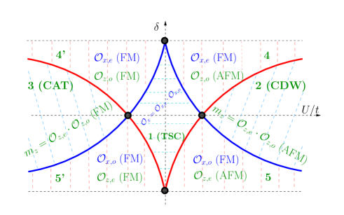
Figure 3: (Color online) Phase diagram of the interacting dimerized Kitaev model with nonvanishing order parameter shown for each phase.

The curves (28,29) shown in Fig. 3 are the phase boundaries, and now we will establish the nature of the order parameters characterizing each of the phases in the $(U/t,\delta)$ parametric plane. The phase diagram of the model was found already in the earlier related work. Ezawa17 ; Miao17b In particular, the winding numbers were calculated, and it was shown that at least one number changes when a phase boundary is crossed, indicating thus topological phase transition(s) along the lines (28,29). This is not surprising, since the phase boundaries are the branching points of the spectra (27). Our goal is to find the Landau-like order parameters for each phase of the diagram. The phases 1-3 in Fig. 3 are continuous extensions of their counterparts found in Miao17a at $\delta=0$.

Region 1 (Topological superconductor (TSC)): In this phase the $\mathbb{Z}_{2}$ symmetry is spontaneously broken in the even and odd sectors of the Hamiltonian (24), the ground state is then 4-fold degenerate, and $m_{x}=\langle\tau^{x}_{e}\rangle\langle\tau^{x}_{o}\rangle$. GT2017 Then we easily find nontrivial Majorana SOP for this phase:

$$\mathcal{O}_{x} = \displaystyle\Big{[}\Big{(}1-\Big{[}\frac{U}{t}\frac{1-\delta}{1+\delta}\Big{]}^{2}\Big{)}\Big{(}1-\Big{[}\frac{U}{t}\frac{1+\delta}{1-\delta}\Big{]}^{2}\Big{)}\Big{]}^{1/8}\leavevmode\nobreak\ ,$$ (31)

$$\mathrm{at}\leavevmode\nobreak\ \leavevmode\nobreak\ \{\delta_{c,e}<\delta<\delta_{c,o}\}\cup\{|U|/t<1\}\leavevmode\nobreak\ .$$

This phase and its order parameter are smoothly connected to the corresponding phase of the free Kitaev chain shown in Fig. 1

Reqions 2 & 3 (CDW & CAT): To calculate the order parameter(s) for those phases we apply the duality transformations (22,23) with the interchange $x\leftrightarrow y$. The Hamiltonian (21) maps again onto a sum of the even and odd transverse Ising chains as:

$$H_{e} = \sum_{l=1}^{N/2}U(1-\delta)\tau_{2l-2}^{y}\tau_{2l}^{y}-t(1+\delta)\tau_{2l}^{z}$$ (32)

$$H_{o} = \sum_{l=1}^{N/2}U(1+\delta)\tau_{2l-1}^{y}\tau_{2l+1}^{y}-t(1-\delta)\tau_{2l-1}^{z}\leavevmode\nobreak\ ,$$ (33)

which have ferromagnetic or antiferromagnetic (depending on the sign of $U$) long-ranged order

$$\langle\tau^{y}_{e/o}\rangle\neq 0\leavevmode\nobreak\ \leavevmode\nobreak\ \mathrm{if}\leavevmode\nobreak\ \leavevmode\nobreak\ \delta\lessgtr\delta_{c,e/o}\leavevmode\nobreak\ .$$ (34)

The order parameter $m_{z}$ is defined via the density correlation function

$$4\langle\delta n_{i}\delta n_{j}\rangle=\langle(2c^{{\dagger}}_{i}c_{i}-1)(2c^{{\dagger}}_{j}c_{j}-1)\rangle$$

$$\leavevmode\nobreak\ \xrightarrow{(j-i)\to\infty}\leavevmode\nobreak\ [-\mathrm{sign}(U)]^{j-i}m_{z}^{2}\leavevmode\nobreak\ ,$$ (35)

where the $z$-component is understood in terms of (19) and (20) before the spin rotation. The nontrivial value of

$$m_{z}=|\langle 2c^{{\dagger}}_{n}c_{n}-1\rangle|=|\langle a_{n}b_{n}\rangle|=|\langle\tau^{y}_{e}\rangle\langle\tau^{y}_{o}\rangle|\leavevmode\nobreak\ .$$ (36)

is given by

$$m_{z} = \displaystyle\Big{[}\Big{(}1-\Big{[}\frac{t}{U}\frac{1+\delta}{1-\delta}\Big{]}^{2}\Big{)}\Big{(}1-\Big{[}\frac{t}{U}\frac{1-\delta}{1+\delta}\Big{]}^{2}\Big{)}\Big{]}^{1/8}\leavevmode\nobreak\ ,$$ (37)

$$\mathrm{at}\leavevmode\nobreak\ \leavevmode\nobreak\ \{\delta_{c,o}<\delta<\delta_{c,e}\}\cup\{|U|/t>1\}\leavevmode\nobreak\ .$$

The phase with alternating density at $U/t>0$ is associated with the charge-density wave (CDW), while the superposition of two differently homogeneously filled states (in our dual representation they are dual even and odd sublattices with distinct ferromagnetic orders $\langle\tau^{y}_{e}\rangle$ and $\langle\tau^{y}_{o}\rangle$) at $U/t<0$ is called the CAT phase. Miao17a (Named after Schrödinger’s cat superposition state.) Similarly to the TSC phase, the CDW and CAT phases have 4-fold degenerate ground states and correspond to the completely broken $\mathbb{Z}_{2}\otimes\mathbb{Z}_{2}$ symmetry.

Regions 4 & 5: Now we introduce two types of rarefied strings IsingCasc and define the even and odd Majorana string operators:

$$O_{x,e}(m)=\prod_{l=1}^{m}\big{[}ib_{2l-1}a_{2l}\big{]}\leavevmode\nobreak\ ,$$ (38)

$$O_{x,o}(m)=\prod_{l=1}^{m}\big{[}ib_{2l}a_{2l+1}\big{]}\leavevmode\nobreak\ .$$ (39)

The corresponding Majorana SOPs are defined similarly to (10). Using the Jordan-Wigner (Local and nonlocal order parameters in the Kitaev chain) and duality transformation (22) we obtain the important relations

$$\mathcal{O}_{x,e/o}^{2}=\lim_{(R-L)\rightarrow\infty}\left<\tau_{L}^{x}\tau_{R}^{x}\right>\leavevmode\nobreak\ ,$$ (40)

where the ends of the strings are chosen such that:

$$L=2n,\leavevmode\nobreak\ R=2m\leavevmode\nobreak\ \longmapsto \leavevmode\nobreak\ \mathcal{O}_{\alpha,e}\leavevmode\nobreak\ ,$$

$$L=2n-1,\leavevmode\nobreak\ R=2m-1\leavevmode\nobreak\ \longmapsto \leavevmode\nobreak\ \mathcal{O}_{\alpha,o}\leavevmode\nobreak\ .$$ (41)

This leads us easily to the nontrivial SOPs for the phases 4 and 5:

$$\mathcal{O}_{x,e/o} = \displaystyle\Big{(}1-\Big{[}\frac{U}{t}\frac{1\mp\delta}{1\pm\delta}\Big{]}^{2}\Big{)}^{1/8}\leavevmode\nobreak\ ,$$ (42)

$$\mathrm{at}\leavevmode\nobreak\ \leavevmode\nobreak\ \{\delta\gtrless\delta_{c,o}\}\cup\{\delta\gtrless\delta_{c,e}\}\leavevmode\nobreak\ .$$

As one can infer from definition (38) and Fig. 2, the appearance of SOP $\mathcal{O}_{x,e}\neq 0$ signals nonvanishing average value of the rarefied string made out of Majorana dimers residing on the same leg of the ladder and coupled by a “plus” bond $t+\delta$. Similarly, the nonvanishing $\mathcal{O}_{x,o}$ probes the rarefied strings made out the “minus” dimers coupled by $t-\delta$. Note that the SOP in the TSC phase $\mathcal{O}_{x}=\mathcal{O}_{x,e}\mathcal{O}_{x,o}$ is a superposition of these two rarefied strings where their nonzero averages overlap. The ground states of the rarefied dimer phases 4 and 5 are two-fold degenerate, and nonvanishing SOPs $\mathcal{O}_{x,e/o}$ signal breaking of one of the $\mathbb{Z}_{2}\otimes\mathbb{Z}_{2}$ symmetries, either in the even or odd sector of the dual Hamiltonian.

Another couple of SOPs in these two phases can be deduced from the local magnetizations (34) on the even/odd dual sublattices (32) and (33) (cf. also (41)):

$$\langle\tau_{L}^{y}\tau_{R}^{y}\rangle=\langle\prod_{l=L+1}^{R}\big{[}-ia_{l}b_{l}\big{]}\rangle$$

$$\leavevmode\nobreak\ \xrightarrow{(R-L)\to\infty}\leavevmode\nobreak\ [-\mathrm{sign}(U)]^{\frac{R-L}{2}}\mathcal{O}_{z,e/o}^{2}\leavevmode\nobreak\ ,$$ (43)

Analytically, we find

$$\mathcal{O}_{z,e/o} = \displaystyle\Big{(}1-\Big{[}\frac{t}{U}\frac{1\pm\delta}{1\mp\delta}\Big{]}^{2}\Big{)}^{1/8}\leavevmode\nobreak\ ,$$ (44)

$$\mathrm{at}\leavevmode\nobreak\ \leavevmode\nobreak\ \{\delta\lessgtr\delta_{c,o}\}\cup\{\delta\lessgtr\delta_{c,e}\}\leavevmode\nobreak\ ,$$

These two SOPs combine into the local order parameter (average density) $m_{z}=\mathcal{O}_{z,e}\mathcal{O}_{z,o}$ in the phases CDW and CAT, where these even and odd SOP coexist.

$\bullet$ Conclusions.– Using spin-fermion and spin-spin duality transformations we have calculated order parameters for the phases of the noninteracting Kitaev chain and for the chain with interaction and dimerization at a special symmetric point. The main building blocks we used are various string operators made out of Majorana fermions. The string order parameters (SOPs) are defined by the asymptotes of the corresponding string correlation functions. Using duality we show that the SOPs are local order parameters of the dual Hamiltonians and are easily calculated. On the phase diagram Ezawa17 ; Miao17b of the interacting dimerized model we have found the nonlocal order detected by the rarefied strings built from selected sets of the Majorana operators (Phases 4 & 5). Such rarefied SOPs coexist in the TSC phase and their overlap results in the SOP which continuously evolves from the corresponding SOP of the noninteracting chain. The phases CAT and CDW possess conventional local order parameters known from the analysis of the interacting model without dimerization. Miao17a Using the duality we have easily obtained the results for those local parameters as products of corresponding overlapping SOPs. Each symmetry broken in a given phase of the model is identified with the spontaneous symmetry breaking of the dual Hamiltonian(s). We have also related the phase transitions of the model (including the disorder line) to zeros of its partition function. Form the results for the gaps and order parameters we infer the critical indices $\nu=1$ and $\beta=1/8$ of the 2D Ising universality class. Note This is valid of course only for the particular symmetry point in the parameter space considered where the interacting model is equivalent to free fermions.

We expect the proposed SOPs to be operational to explore the model’s phase diagram away from this special point, EzawaNagaosa14 ; Zeng16 ; Miao17a ; Ezawa17 ; Miao17b when the fermionic interactions need to be dealt with. This can be done along the lines of our earlier related work on spin ladders (i.e. interacting fermions). GT2017 ; UsLadd Another interesting extension is the noninteracting Kitaev chain with long-ranged superconducting pairing, which has a quite nontrivial phase diagram and very interesting critical properties.LRpairing These are very promising and relatively straightforward directions for advancement of the present formalism, which we relegate for future work.

Appendix A Critical and disorder lines, Lee-Yang zeros, and Majorana edge states in the $XY$ model

Since the seminal papers by Yang and Lee LeeYang52 we are able to rigorously relate phase transitions in a model to zeros of its partition function. Such zeros in the $1D$ $XY$ model and its integrable deformations which keep the Hamiltonian equivalent to free fermions, were analyzed in Tong06 . (See also Tong12 for a follow-up work). In units of $J$ the Hamiltonian of the model is

$$H=-\frac{1}{2}\sum_{i=1}^{N}\bigg{\{}\frac{1}{2}\big{(}1+\gamma\big{)}\sigma_{i}^{x}\sigma_{i+1}^{x}+\frac{1}{2}\big{(}1-\gamma\big{)}\sigma_{i}^{y}\sigma_{i+1}^{y}+h\sigma_{i}^{z}\bigg{\}}\leavevmode\nobreak\ .$$ (45)

The partition function

$$\mathcal{Z}(h,\gamma,T;\{k\})=\prod_{k\in[0,2\pi]}e^{\beta\varepsilon(k)/2}\Big{(}e^{-\beta\varepsilon(k)}+1\Big{)}\leavevmode\nobreak\ .$$ (46)

has its zeros determined from the following equation:Tong06

$$\varepsilon(k)=\sqrt{(h-\cos k)^{2}+\gamma^{2}\sin^{2}k}=i(2n+1)\pi T\leavevmode\nobreak\ ,$$ (47)

(we set $k_{B}=1$) resulting in the solution with a complex magnetic field

$$h=\cos k\pm i\sqrt{\gamma^{2}\sin^{2}k+(2n+1)^{2}\pi^{2}T^{2}}\leavevmode\nobreak\ .$$ (48)

At zero temperature the Lee-Yang zeros are also zeros of the spectrum, and they are located on the ellipse in the plane $h=h^{\prime}+ih^{\prime\prime}\in\mathbb{C}$:

$$(h^{\prime})^{2}+\bigg{(}\frac{h^{\prime\prime}}{\gamma}\bigg{)}^{2}=1\leavevmode\nobreak\ .$$ (49)

The Lee-Yang zeros located on the real axis of the complex magnetic plane are the points of quantum criticality. For arbitrary $\gamma\neq 0$ this gives us to lines of the quantum phase transitions $h=\pm 1$, while for $\gamma=0$ the ellipse collapses into the critical line $h\in[-1,1]$. Thus predictions for the phase boundaries of the Lee-Yang formalism reproduce the results known from analysis of the correlation functions,Barouch71 as it must be.

A more interesting question is to understand the origin of the transition on the disorder line

$$h^{2}+\gamma^{2}=1\leavevmode\nobreak\ ,$$ (50)

where there is no gap closure, and the transition is detected by the change of asymptotic behavior of the spin correlation functions: the exponentially decaying functions acquire additional oscillations inside the circle (50).Barouch71 The ground state energy

$$E_{0}=-\frac{N}{2\pi}\int_{0}^{\pi}dk\varepsilon(k)\leavevmode\nobreak\ ,$$ (51)

is found in terms of elliptical functions Taylor85 and is shown Mac16 to be smooth and even infinitely differentiable function on the boundary (50).

It is convenient to write the spectrum $\varepsilon(k)$ in terms of the complex variable $z=e^{ik}$ as Franchini2017

$$\varepsilon^{2}(z)=\frac{(1+\gamma)^{2}}{4}(z-\lambda_{+})(z-\lambda_{-})(z^{-1}-\lambda_{+})(z^{-1}-\lambda_{-})\leavevmode\nobreak\ ,$$ (52)

where

$$\lambda_{\pm}=\frac{h\pm\sqrt{h^{2}+\gamma^{2}-1}}{1+\gamma}\leavevmode\nobreak\ .$$ (53)

The quantum phase transitions in the $XY$ model we discussed above are signalled by the zeros $\lambda_{\pm}$ of the partition function $\mathcal{Z}(h,\gamma,T\to 0;\{z\})$ lying on the unit circle $|z|=1$. Analytical continuation $k\rightarrowtail k+ik_{0}$ extends the product in the partition function (46) over the complex loop of arbitrary radius $e^{-k_{0}}$, which, in particular, can pass through the roots $\lambda_{\pm}^{\pm 1}$. Thus, the latter are zeros of the zero-temperature partition function analytically continued onto the complex states $|z|\neq 1$. On the other hand, $\lambda_{\pm}$ control the asymptotes of the correlation functions calculated from the Toeplitz determinants McCoyBook ; Franchini2017 . The transition on the disorder line (50) resulting in the oscillations corresponds to the points where $\lambda_{\pm}$ acquire imaginary parts and $\lambda_{+}=\lambda_{-}^{\ast}$. This is in a close analogy to the transition on the disorder line in the classical Ising chain which corresponds to the Lee-Yang zeros in the range of complex parameters.IsingCasc

There is even a more close analogy between the transitions on the disorder lines in the classical Stephenson70 ; IsingCasc and the quantum transverse $XY$ chains. To reveal it one needs to find the zero-energy localized state in the ordered phase $h<1$ of the model Hamiltonian (45). This problem was originally solved by Karevski Karevski00 whose transfer-matrix approach we will follow. (The solution was repeated in more recent literature DeGottardi11 .) The Bogoliubov-de Gennes equation for the Jordan-Wigner fermions in the direct space (cf. equations (1), (4) and (7) ) can be written as

$$\left(\begin{array}[]{cc}0&\hat{A}-\hat{B}\\ \hat{A}+\hat{B}&0\\ \end{array}\right)\leavevmode\nobreak\ \left(\begin{array}[]{c}\Phi_{q}\\ \Psi_{q}\\ \end{array}\right)=\varepsilon(q)\left(\begin{array}[]{c}\Phi_{q}\\ \Psi_{q}\\ \end{array}\right)\leavevmode\nobreak\ ,$$ (54)

where $\hat{A}$ and $\hat{B}$ are $N\times N$ symmetric and antisymmetric matrices, respectively:

$$A_{ij} = 2h\delta_{i,j}+\delta_{i,j+1}+\delta_{i,j-1}$$ (55)

$$B_{ij} = -\gamma\delta_{i,j+1}+\gamma\delta_{i,j-1}\leavevmode\nobreak\ ,$$ (56)

$\Phi_{q}=(\phi_{q}(1)....\phi_{q}(N))^{T}$ and $\Psi_{q}=(\psi_{q}(1)....\psi_{q}(N))^{T}$ are the $N$-component spinors defining the Bogoliubov transformation of the Majorana fermions $(a_{n},b_{n})\mapsto(\alpha_{q},\beta_{q})$ as

$$2\eta_{q}^{\dagger}=\alpha_{q}+i\beta_{q}=\sum_{n=1}^{N}\Big{[}\phi_{q}(n)a_{n}+i\psi_{q}(n)b_{n}\Big{]}\leavevmode\nobreak\ .$$ (57)

In terms of the Bogoliubov fermions $\eta_{q}$ the Hamiltonian is diagonal:

$$H=\sum_{k}\varepsilon(k)\big{[}\eta_{k}^{\dagger}\eta_{k}-\frac{1}{2}\big{]}\leavevmode\nobreak\ .$$ (58)

The energy of the first excited singe-particle state $|1\rangle=\eta_{1}^{\dagger}|GS\rangle$ vanishes in the thermodynamic limit and this state becomes degenerate with the ground state in the ordered phase $h<1$. The wave function $\Phi_{1}$ of the Majorana fermion in this state is found via iteration of the “transfer matrix”

$$\hat{T}=\left(\begin{array}[]{cc}\frac{2h}{1+\gamma}&\frac{1-\gamma}{1+\gamma}\\ -1&0\\ \end{array}\right)$$ (59)

as

$$\phi_{1}(n+1)=(-1)^{n}(\hat{T}^{n})_{11}\phi_{1}(1)\leavevmode\nobreak\ .$$ (60)

The roots (53) also happen to be the eigenvalues of the “transfer matrix”. The latter can be written via two orthogonal idempotent operators (projectors) $\hat{\mathcal{P}}_{\pm}$ as Lancaster69

$$\hat{T}=\lambda_{+}\hat{\mathcal{P}}_{+}+\lambda_{-}\hat{\mathcal{P}}_{-}\leavevmode\nobreak\ ,$$ (61)

where

$$\hat{\mathcal{P}}_{\pm}\equiv\pm\frac{\hat{T}-\lambda_{\mp}\hat{\mathbb{1}}}{\lambda_{+}-\lambda_{-}}\leavevmode\nobreak\ .$$ (62)

Then $\hat{T}^{n}=\lambda_{+}^{n}\hat{\mathcal{P}}_{+}+\lambda_{-}^{n}\hat{\mathcal{P}}_{-}$, and we recover the result of Karevski: Karevski00

$$\phi_{1}(n+1)=(-1)^{n}\frac{\lambda_{+}^{n}-\lambda_{-}^{n}}{\lambda_{+}-\lambda_{-}}\phi_{1}(1)\leavevmode\nobreak\ .$$ (63)

The wave function is delocalized when $h>1$, while in the ordered phase when $h<1$ it is localized near the left edge of the chain $n=1$, and the probability density for this zero-energy edge Majorana fermion exponentially decays with the distance $\phi_{1}^{2}(n\gg 1)\propto\exp(-\kappa n)$. The inverse penetration depth $\kappa=2|\log\lambda_{+}|$ is also the inverse bulk correlation length of the spin correlation function. Barouch71 Inside the disorder circle (50) $\lambda_{+}=\lambda_{-}^{\ast}$ with $|\lambda_{\pm}|^{2}=(1-\gamma)/(1+\gamma)$, the edge-state wavefunction (63) acquires incommensurate oscillations on the top of the exponential decay. The disorder line corresponds to a “weak” continuous phase transition where the correlation length stays finite. As in the classical Ising chain,Stephenson70 it demonstrates a cusp at the critical point. One can check that $\kappa$ as a function of field, approaches its maximum on the disorder line with an infinite slope and stays constant $\kappa=-\log\frac{1-\gamma}{1+\gamma}$ in the oscillating phase. It is natural to identify the localized zero-energy edge-state with the Majorana fermion ($a_{1}$) “missed” by the ordered Majorana string ($\mathcal{O}_{x}\neq 0$) discussed in the main text on the free Kitaev chain.

Since $\lambda_{\pm}(-\gamma)\lambda_{\mp}(\gamma)=1$, the second solution of (54) follows easily

$$\psi_{1}(n+1)=(-1)^{n}\frac{\lambda_{-}^{-n}-\lambda_{+}^{-n}}{\lambda_{-}^{-1}-\lambda_{+}^{-1}}\psi_{1}(1)\leavevmode\nobreak\ .$$ (64)

In the ordered phase this wave function localized near the right edge DeGottardi11 $\psi_{1}(n\gg 1)\sim\psi(N))\exp(-(N-n)|\log\lambda_{-}|)$, acquires oscillations after crossing the disorder line. It can be related to the zero-energy edge-state of the Majorana fermion $b_{N}$. In the range of negative $\gamma$ the solutions interchange in the obvious way, along with $(a_{1},b_{N})\leftrightarrow(b_{1},a_{N})$.

References

- (1) L.D. Landau and E.M. Lifshitz, Statistical Physics Part 1. Course of Theoretical Physics Vol. 5 (3rd ed.), Butterworth-Heinemann (1980).
- (2) E. Fradkin, Field Theories of Condensed Matter Physics, 2nd edition (Cambridge University Press, New York, 2013).
- (3) B.A. Bernevig and T.L. Hughes, Topological Insulators and Topological Superconductors (Princeton University Press, Princeton, 2013).
- (4) S. Ryu, A.P. Schnyder, A. Furusaki, and A.W.W. Ludwig, New J. Phys. 12, 065010 (2010).
- (5) A. Montorsi and M. Roncaglia, Phys. Rev. Lett. 109, 236404 (2012).
- (6) X.-G. Wen, Rev. Mod. Phys. 89, 041004 (2017).
- (7) G.Y. Chitov and T. Pandey, J. Stat. Mech. (2017) 043101.
- (8) J.B. Kogut, Rev. Mod. Phys. 51, 659 (1979).
- (9) M. den Nijs and K. Rommelse, Phys. Rev. B 40, 4709 (1989).
- (10) M. Oshikawa, J. Phys. Condens. Matt. 4, 7469 (1992); T. Kennedy and H. Tasaki, Phys. Rev. B 45, 304 (1992); M. Kohmoto and H. Tasaki, Phys. Rev. B 46, 3486 (1992).
- (11) H.-D. Chen and J. Hu, Phys. Rev. B 76, 193101 (2007).
- (12) X.-Y. Feng, G.-M. Zhang, and T. Xiang, Phys. Rev. Lett. 98, 087204 (2007).
- (13) H.-D. Chen and Z. Nussinov, J. Phys. A: Math. Theor. 41, 075001 (2008); E. Cobanera, G. Ortiz, and Z. Nussinov Phys. Rev. B 87, 041105(R) (2013).
- (14) B.L. Pasternak, Poetry, (G. P. Putnam’s Sons, New York, 1959).
- (15) S.J. Gibson, R. Meyer, and G.Y. Chitov, Phys. Rev. B 83, 104423 (2011); G.Y. Chitov, B.W. Ramakko, and M. Azzouz, Phys. Rev. B 77, 224433 (2008); M. Azzouz, K. Shahin, and G.Y. Chitov, Phys. Rev. B 76, 132410 (2007).
- (16) A. Kitaev, Usp. Fiz. Nauk (Suppl.) 171, 131 (2001).
- (17) F. Franchini, An Introduction to Integrable Techniques for One-Dimensional Quantum Systems, Lecture Notes in Physics 940, (Springer, Heidelberg, 2017).
- (18) E.H. Lieb, T. Schultz, and D. Mattis, Ann. Phys. (N.Y.) 16, 407 (1961).
- (19) W. DeGottardi, D. Sen, and S. Vishveshwara, New J. Phys. 13, 065028 (2011).
- (20) E. Barouch and B.M. McCoy, Phys. Rev. A 3, 786 (1971).
- (21) R. Wakatsuki, M. Ezawa, Y. Tanaka, and N. Nagaosa, Phys. Rev. B 90, 014505 (2014).
- (22) Q.-B. Zeng, S. Chen, R. Lü, Phys. Rev. B 94, 125408 (2016).
- (23) J.-J. Miao, H.-K. Jin, F.-C. Zhang, and Y. Zhou, Phys. Rev. Lett. 118, 267701 (2017).
- (24) M. Ezawa, Phys. Rev. B 96, 121105(R) (2017).
- (25) Y. Wang, J.-J. Miao, H.-K. Jin, and S. Chen, Phys. Rev. B 96, 205428 (2017).
- (26) J.H.H. Perk, H.W. Capel, M.J. Zuilhof, and Th. J. Siskens, Physica A 81, 319 (1975).
- (27) F. Ye, G.-H. Ding, and B.-W. Xu, Commun. Theor. Phys. (Beijing, China) 37, 492 (2002); F. Ye and B.-W. Xu, Commun. Theor. Phys. (Beijing, China) 39, 487 (2003).
- (28) E. Fradkin and L. Susskind, Phys. Rev. D 17, 2637 (1978).
- (29) H.W. Capel and J.H.H. Perk, Physica A 87, 211 (1977). For more literature and a recent overview on such transformation and factorization, J.H.H. Perk, arXiv:1710.03384.
- (30) P. Pfeuty, Ann. Phys. (N.Y.) 57, 79 (1970).
- (31) The exception is limit of the noninteracting model which corresponds to the isotropic limit of the model. It is known Franchini2017 to belong to the different universality class of the conformal charge . (The Ising belongs to the class).
- (32) C.N. Yang and T.D. Lee, Phys. Rev. 87, 404 (1952); T.D. Lee and C.N. Yang, Phys. Rev. 87, 410 (1952).
- (33) P. Tong and X. Liu, Phys. Rev. Lett. 97, 017201 (2006).
- (34) X. Liu, M. Zhong, H. Xu, and P. Tong, J. Stat. Mech. P01003 (2012).
- (35) B.M. McCoy, Advanced Statistical Mechanics (Oxford University Press, New York, 2010).
- (36) J.H. Taylor and G. Müller, Physica A 130, 1 (1985).
- (37) T. Maciazek and J. Wojtkiewicz, Physica A 441, 131 (2016).
- (38) J. Stephenson, Can. J. Phys. 48, 1724 (1970); Phys. Rev. B 1, 4405 (1970).
- (39) P.N Timonin and G.Y. Chitov, Phys. Rev. E 96, 062123 (2017).
- (40) D. Karevski, J. Phys. A: Math. Theor. 33, L313 (2000).
- (41) D. Vodola, L. Lepori, E. Ercolessi, and G. Pupillo, New J. Phys. 18, 015001 (2016); L. Lepori and L. Dell’Anna, ibid 19, 103030 (2017); L. Lepori, A. Trombettoni, and D. Vodola, J. Stat. Mech. (2017) 033102.
- (42) P. Lancaster, Theory of Matrices (Academic Press, New York, 1969).