Dynamics of vaccination in a time-delayed epidemic model with awareness

Abstract

This paper investigates the effects of vaccination on the dynamics of infectious disease, which is spreading in a population concurrently with awareness. The model considers contributions to the overall awareness from a global information campaign, direct contacts between unaware and aware individuals, and reported cases of infection. It is assumed that there is some time delay between individuals becoming aware and modifying their behaviour. Vaccination is administered to newborns, as well as to aware individuals, and it is further assumed that vaccine-induced immunity may wane with time. Feasibility and stability of the disease-free and endemic equilibria are studied analytically, and conditions for the Hopf bifurcation of the endemic steady state are found in terms of system parameters and the time delay. Analytical results are supported by numerical continuation of the Hopf bifurcation and numerical simulations of the model to illustrate different types of dynamical behaviour.

1 Introduction

Vaccines are known to be effective means of disease control and prevention [13, 19, 24, 42], having led to a complete eradication of smallpox [6, 28] and a substantial reduction in the cases of polio, measles, mumps, rubella. Latest WHO forecasts suggest expected eradication of measles and mumps in Europe in the next few years [49]. Depending on a particular disease and each individual vaccine, the vaccine-induced immunity may be life-long, or individuals may require subsequent vaccinations to improve their immunity status. In order to achieve maximum impact, every vaccination campaign should be accompanied by appropriate information campaigns that educate individuals about the need for vaccination to prevent the spread of infection and achieve the desired level of herd immunity [24]. In some cases, negative press coverage has led to a reduction in vaccine uptake or even complete disruption of the vaccination campaign, as has been the case with HPV vaccine in Romania [36] and the MMR vaccine in the UK [8]. Furthermore, fears associated with possible side effects or incorrect perceptions about vaccine efficiency may also be detrimental to the vaccine uptake and subsequent success [5, 43].

A number of mathematical models have looked into the dynamics of vaccination [4, 5, 11, 22, 24, 26, 39, 44] focusing on different types of vaccination schedules, various scenarios of vaccine uptake and efficiency, and the resulting control of epidemics. Some work has also been done on developing techniques for assessment and quantification of vaccine efficacy and efficiency [13, 19, 42]. More recently, attention has turned to vaccination models that include different types of population awareness [28, 41, 46] and/or time delays due to either epidemiological properties of infection, such as latency or temporary immunity, or time delay in individuals’ responses to available information about the disease [1, 27, 32, 40]. Liu et al. [30] have recently discussed an interesting notion of “endemic” bubble in the context of delayed behavioural response during epidemics, which corresponds to existence of periodic oscillations around the endemic steady state only for some finite range of basic reproduction numbers.

In this paper we focus on the interactions between two approaches to reducing population-level impact of an infectious disease: spread of awareness and vaccination. The literature on epidemic models of the concurrent spread of disease and information is quite substantial, and mostly consists of mean-field [3, 14, 17, 25, 31] or network models [15, 14, 16, 18, 21, 23, 37, 48, 50]. Within the set of mean-field models, disease awareness can be treated as an additional “media” variable [33, 35, 38] or incorporated into reduced rates of disease transmission [9, 10, 28, 29, 45, 47, 46]. Since there are several distinct contribution to the overall disease awareness that come from contacts between unaware and aware individuals, global awareness campaigns, or reports of the incidence of infection, it is often realistic to include in the models time delays that are associated with either delayed reporting of infected cases or delayed responses of individuals to available information about the disease [17, 34, 51, 52, 53].

Zhao et al. [51] have modelled the delay in media coverage of an epidemic outbreak as a delayed term acting to reduce the disease transmission rate. Greenhalgh et al. [17] have explicitly incorporated in their model a separate compartment for a level of disease awareness, and considered the effects of two time delays on epidemic dynamics, one associated with the “forgetting time”, i.e. the time it takes for the aware susceptible individuals to become unaware again, and the other being the time it takes for awareness to emerge from the infected cases being reported. Similar approach has been pursued by Zuo et al. [52, 53] who included the time delay in reporting of cases either through a delayed awareness term [52], or a delayed contribution from the infected cases to the growth of population awareness [53]. Very recently, Agaba et al. [2] have proposed and studied a model, in which population awareness increases due to global campaigns, as well as reported cases of infection, and a contribution from aware susceptible individuals. In this model, the time delay associated with delayed response of individuals to available information can lead to a destabilisation of endemic steady state and subsequent onset of stable periodic oscillations. Whilst these models have provided insights into epidemic dynamics with account for disease awareness and time delays associated with reporting of cases or modifying the behaviour, they did not consider the effects of epidemic control or vaccination.

In terms of analysis of control of epidemics in time-delayed models, Meng et al. [32] and Sekiguchi and Ishiwata [40] have considered the influence of pulse vaccination on dynamics of SIR epidemic models with time delay representing disease incubation time. Abta et al. [1] have studied a similar problem from the control theory point of view, and showed how optimal control of epidemics can be achieved. The main emphasis of these models was on the effects of vaccination on epidemics, in which some aspects of the disease transmission were delayed, but they did not make any account for disease awareness.

In this paper, we consider the effects of vaccination in an epidemic model with awareness. Of particular interest is the interplay between parameters characterising the emergence of disease awareness, the time delay associated with individuals’ response to available information about the disease, and the levels of vaccination. The paper is organised as follows. In the next Section we introduce a time-delayed model of disease dynamics in the presence of awareness and vaccination, and establish the well-posedness of this model. Section 3 contains analytical results of feasibility and stability analyses of the disease-free and endemic equilibria, together with conditions for a Hopf bifurcation of the endemic steady state. Section 4 is devoted to a numerical bifurcation analysis and simulations that illustrate behaviour of the model in different dynamical regimes. The paper concludes in Section 5 with the discussion of results and open problems.

2 Model derivation

We begin by considering an SIRS-type model, which is a modification of the model analysed recently in Agaba et al. [2]. Unlike that earlier model, we now include vital dynamics (though the disease is still assumed to be non-lethal) and assume that vaccination may not confer a life-long immunity. The population is divided into groups of susceptible individuals unaware of infection, $S_{n}(t)$, susceptible individuals aware of infection, $S_{a}(t)$, infected individuals $I(t)$, and recovered individuals $R(t)$. There is a constant birth rate $b$, which is taken to be the same as the death rate, so that the total population $N$ remains constant, and it is assumed that all newborns are unaware and susceptible to infection. The disease is transmitted from infected to unaware susceptible individuals at a rate $\beta$, and this rate is reduced by a factor $0<\sigma_{s}<1$ for aware susceptibles, who take some measures to reduce their potential contact rate. Infected individuals recover at a rate $r$. Disease awareness $M(t)$ has contributions from the reported number of cases at a rate $\alpha_{o}$, from the aware individuals at a rate $\alpha$, and from some global awareness campaigns at a rate $\omega_{o}$, and the awareness is lost at a rate $\lambda_{o}$, whereas aware susceptibles lose their awareness at a rate $\lambda$. Finally, unaware susceptibles become aware at a rate $\eta$, and it is assumed that it takes time $\tau$ for them to become aware or to modify their behaviour in the relation to spreading infection. These assumptions lead to the following basic model

$$\begin{array}[]{l}\displaystyle{S_{n}^{\prime}=bN-\frac{\beta IS_{n}}{N}-\eta M(t-\tau)S_{n}+\lambda S_{a}-bS_{n},}\\ \\ \displaystyle{S_{a}^{\prime}=-\frac{\sigma_{s}\beta IS_{a}}{N}+\eta M(t-\tau)S_{n}-\lambda S_{a}-bS_{a},}\\ \\ \displaystyle{I^{\prime}=\frac{\beta IS_{n}}{N}+\frac{\sigma_{s}\beta IS_{a}}{N}-rI-bI,}\\ \\ \displaystyle{R^{\prime}=rI-bR,}\\ \\ \displaystyle{M^{\prime}=\omega_{o}+\alpha_{o}I+\frac{\alpha S_{a}}{N}-\lambda_{o}M,}\end{array}$$ (1)

where $S_{n}(t)+S_{a}(t)+I(t)+R(t)=N={\rm const}$. A summary of model parameters is given in Table 1.

Parameter	Definition
$b$	birth rate (same as the death rate)
$\beta$	disease transmission rate
$\sigma_{s}$	rate of reduction in susceptibility to infection due to being aware
$r$	recovery rate
$\alpha_{o}$	growth rate of disease awareness from the reported number of infections
$\alpha$	growth rate of disease awareness arising from aware individuals
$\omega_{o}$	growth rate of disease awareness from global awareness campaigns
$\lambda_{o}$	rate of loss of awareness generated by awareness dissemination
$\lambda$	rate of loss of awareness in susceptible individuals

Table 1: Parameter definitions

To investigate the effects of the introduction of a vaccine on the disease dynamics, we consider a situation where a proportion $v$ of newborns are vaccinated, and aware susceptible individuals are vaccinated at the rate $v_{s}$. With this assumption, $bvN\equiv v_{i}N$ newborns appear straight in the recovered (protected) class, and $b(1-v)N=(b-v_{i})N$ newborns go to the class of unaware susceptibles. Note that the newborn vaccination is considered to be constant since infants, assumed to be unaware, are vaccinated as a result of awareness of their parents, as well as nurses/doctors. Once they become aware of infection as adults, that automatically classifies them as aware susceptibles that could then be influenced by the awareness campaign for enhancing vaccination courage. It is further assumed that after a period of time $1/\delta$, the individuals lose their immunity against the infection. If $\delta=0$, this describes a perfect vaccine, while $\delta>0$ describes a vaccine resulting in temporary (waning) immunity. Similar to some earlier works [2, 52, 53], it is assumed that upon losing immunity, a certain proportion, $p$, of individuals will join the aware susceptible class while the remaining proportion, $q=1-p$, will return to the unaware susceptible class. With these assumptions, a modified model has the form

$$\begin{array}[]{l}\displaystyle{S_{n}^{\prime}=(b-v_{i})N-\frac{\beta IS_{n}}{N}-\eta M(t-\tau)S_{n}+\lambda S_{a}+\delta qR-bS_{n},}\\ \\ \displaystyle{S_{a}^{\prime}=-\frac{\sigma_{s}\beta IS_{a}}{N}+\eta M(t-\tau)S_{n}-(\lambda+v_{s}+b)S_{a}+\delta pR,}\\ \\ \displaystyle{I^{\prime}=\frac{\beta IS_{n}}{N}+\frac{\sigma_{s}\beta IS_{a}}{N}-(r+b)I,}\\ \\ \displaystyle{R^{\prime}=rI+v_{i}N+v_{s}S_{a}-(\delta+b)R,}\\ \\ \displaystyle{M^{\prime}=\omega_{o}+\alpha_{o}I+\frac{\alpha S_{a}}{N}-\lambda_{o}M.}\end{array}$$ (2)

This system has to be augmented by an appropriate initial conditions

$$\begin{array}[]{l}S_{n}(0)=S_{n_{0}}\geq 0,\quad S_{a}(0)=S_{a_{0}}\geq 0,\quad I(0)=I_{0}>0,\quad R(0)=R_{0}\geq 0,\\ \\ M(0)=M_{0}\geq 0,\qquad M(s)=M_{0}(s)\geq 0\qquad\text{for all}\quad s\in[-\tau,0).\end{array}$$ (3)

Before proceeding with the analysis of the model (2), it is essential to verify that it is feasible, i.e. its solutions remain non-negative and bounded for all $t\geq 0$.

Theorem 1.

The solutions $(S_{n}(t),S_{a}(t),I(t),R(t),M(t))$ of the system (2) with the initial condition (3) are non-negative and bounded for all $t\geq 0$.

Proof. Considering the equation for $I(t)$, let $t_{i}>0$ be the first time when $I(t)=0$, and the other components are still non-negative as per initial conditions, so

$$S_{n}(t)\geq 0,\quad S_{a}(t)\geq 0\qquad\text{for all}\quad t\in[0,t_{i}].$$

Introducing an auxiliary quantity

$$\psi=\min_{0\leq t\leq t_{i}}\left\{\frac{\beta S_{n}}{N}+\frac{\sigma_{s}\beta S_{a}}{N}-(r+b)\right\},$$

we have the relation

$${I^{\prime}=\frac{\beta IS_{n}}{N}+\frac{\sigma_{s}\beta IS_{a}}{N}-(r+b)I\geq\psi I,}$$

that can be readily solved to yield

$$I(t_{i})\geq I(0)e^{\psi t_{i}}>0,$$

which gives a contradiction.

In a similar way, let us assume there exists a first time $t_{n}>0$ such that $S_{n}(t)>0$ for $t\in[0,t_{n})$ and $S_{n}(t_{n})=0$, which implies $dS_{n}(t_{n})/dt<0$. Substituting this value of $S_{n}$ into the first equation of the system (2) gives

$$\frac{dS_{n}}{dt}\Big{|}_{t=t_{n}}=(b-v_{i})N+\lambda S_{a}+\delta qR>0,$$

which contradicts the initial assumption. Consequently, $S_{n}(t)>0$ for $t\geq 0$, and similar arguments can be used to establish that $S_{a}$, $R$ and $M$ remain non-negative for all $t\geq 0$.

Having established the positivity of all state variables, from the fact that $S_{n}(t)+S_{a}(t)+I(t)+R(t)=N={\rm const}$, it immediately follows that they are also all bounded between $0$ and $N$. Looking at the last equation of the system (2), we have

$$M^{\prime}=\omega_{o}+\alpha_{o}I+\frac{\alpha S_{a}}{N}-\lambda_{o}M\leq\omega_{o}+\alpha_{o}N+\alpha-\lambda_{o}M,$$

which can be solved to give

$${M(t)\leq M(0)e^{-\lambda_{o}t}+\frac{\omega_{o}+\alpha_{o}N+\alpha}{\lambda_{o}}\left(1-e^{-\lambda_{o}t}\right)\leq\widehat{M},}$$

where

$${\widehat{M}=M(0)+\frac{\omega_{o}+\alpha_{o}N+\alpha}{\lambda_{o}}.}$$ (4)

This suggests that throughout the time evolution, all solutions remain within the bounded region

$$\Phi=\left\{(S_{n},S_{a},I,R,M)\in\mathbb{R}_{+}^{5}:0\leq S_{n},S_{a},I,R\leq N,0\leq M\leq\widehat{M}\right\}.$$

$\blacksquare$

3 Steady states and their stability

The system (2) can have at most two steady states, a disease-free equilibrium and an endemic equilibrium. The disease-free steady state is given by

$$E_{0}=(S_{n}^{\circ},S_{a}^{\circ},0,R^{\circ},M^{\circ}).$$

where

$$S_{n}^{\circ}=Nh_{n},\quad S_{a}^{\circ}=Nh_{a},\quad R^{\circ}=N(1-h_{a}-h_{n}),\quad M^{\circ}=\frac{\omega_{o}+\alpha h_{a}}{\lambda_{o}},$$ (5)

and

$${h_{a}=\frac{-x_{2}+\sqrt{x_{2}^{2}+4x_{1}x_{3}}}{2x_{1}},\quad h_{n}=\frac{\lambda_{o}[b-v_{i}+\delta q(1-h_{a})+\lambda h_{a}]}{\eta(\omega_{o}+\alpha h_{a})+\lambda_{o}(\delta q+b)},}$$

with

$$\begin{array}[]{l}x_{1}=\eta\alpha(\delta+v_{s}+b),\\ \\ x_{2}=\lambda_{o}(\delta+b)(\lambda+b)+\lambda_{o}v_{s}(\delta q+b)+\eta\omega_{o}(\delta+v_{s}+b)-\eta\alpha(b+\delta-v_{i}),\\ \\ x_{3}=\lambda_{o}\delta pv_{i}+\eta\omega_{o}(b+\delta-v_{i}).\end{array}$$

The steady state $E_{0}$ is biologically feasible, as long as the following condition holds

$$h_{a}<\frac{b+\delta-v_{i}}{\delta+v_{s}+b},$$ (6)

which also implies $0<h_{n}<1$. Due to the fact that $h_{a}$ is monotonically increasing with $\omega_{o}$, we have

$$0<h_{a}(\omega_{o}=0)<h_{a}<h_{a}(\omega_{o}=\infty)<\frac{b+\delta-v_{i}}{\delta+v_{s}+b},$$

implying that a condition (6) is always satisfied, so the disease-free steady state $E_{0}$ is biologically feasible for all values of parameters. Unlike $h_{a}$, $h_{n}$ is monotonically decreasing with $\omega_{o}$, and the same behaviour is exhibited by $h_{a}$ and $h_{n}$ in their dependence on $\alpha$. In fact, for large $\alpha$, $h_{n}\to 0$, while $h_{a}\to(b+\delta-v_{i})/(\delta+v_{s}+b)$. An explanation for this is that increasing $\alpha$ leads to the growth of $M(t)$, which, in turn, results in the majority of susceptible individuals being aware, and they then contribute to further growth of $M(t)$ in a manner similar to the effect of a global awareness campaign.

The endemic equilibrium $E^{*}=(S_{n}^{*},S_{a}^{*},I^{*},R^{*},M^{*})$ is given by

$$\begin{array}[]{l}\displaystyle{S_{n}^{*}=Nh_{n_{*}},\quad S_{a}^{*}=Nh_{a_{*}},\quad I^{*}=Nh_{i_{*}},}\\ \\ \displaystyle{R^{*}=N(1-h_{n_{*}}-h_{a_{*}}-h_{i_{*}}),\quad M^{*}=\frac{Nh_{i_{*}}\alpha_{o}+\omega_{o}+\alpha h_{a_{*}}}{\lambda_{o}},}\end{array}$$ (7)

with

$$h_{n_{*}}=\frac{y_{2}\pm\sqrt{y_{2}^{2}-4y_{1}y_{3}}}{2y_{1}},\quad h_{a_{*}}=\frac{r+b-\beta h_{n_{*}}}{\sigma_{s}\beta},\qquad h_{i_{*}}=\frac{h_{n_{*}}(m_{1}h_{n_{*}}-m_{6})+m_{7}}{\sigma_{s}\beta(\lambda_{o}\delta q+m_{4}h_{n_{*}})},$$

where

$$\begin{array}[]{l}m_{1}=\beta\eta\alpha,\quad m_{2}=\beta\lambda_{o}[\lambda+v_{s}+b+\delta p(1-\sigma_{s})]+\eta\alpha(r+b)+\sigma_{s}\beta\eta\omega_{o},\\ \\ m_{3}=\lambda_{o}[(\lambda+\delta p+v_{s}+b)(r+b)-\sigma_{s}\beta\delta p],\quad m_{4}=N\eta\alpha_{o}+\beta\lambda_{o},\\ \\ m_{5}=\lambda_{o}(r+\delta p+b),\quad m_{6}=\beta\lambda_{o}(\lambda+\sigma_{s}\delta q+\sigma_{s}b-\delta q)+\sigma_{s}\beta\eta\omega_{o}+\eta\alpha(r+b),\\ \\ m_{7}=\lambda_{o}[\sigma_{s}\beta(b+\delta q-v_{i})+(\lambda-\delta q)(r+b)],\end{array}$$

and

$$\begin{array}[]{l}y_{1}=m_{1}(\lambda_{o}\delta q+m_{5})+m_{4}(m_{6}-m_{2}),\quad y_{2}=\lambda_{o}\delta qm_{2}+m_{5}m_{6}+m_{4}(m_{7}-m_{3}),\\ \\ y_{3}=\lambda_{o}\delta qm_{3}+m_{5}m_{7}.\end{array}$$

The endemic steady state $E^{*}$ is biologically feasible, provided $0<h_{n_{*}}<(r+b)/\beta$.

Since the total population is constant, one can remove the equation for $R(t)$ and focus on the behaviour of variables $S_{n}(t)$, $S_{a}(t)$ and $I(t)$ only, with $R(t)=N-S_{n}(t)-S_{a}(t)-I(t)$. This reduces the total number of equations without affecting the system dynamics. We begin stability analysis of these steady states by looking at the disease-free equilibrium.

Theorem 2.

The disease-free equilibrium of the system (3) is linearly asymptotically stable for all $\tau\geq 0$ if the basic reproductive number satisfies the condition $R_{v}^{d}<1$, where

$$R_{v}^{d}=\frac{\beta(h_{n}+\sigma_{s}h_{a})}{r+b}.$$ (8)

Proof. For $\tau=0$, application of the next generation matrix method [12] immediately yields the result of the Theorem.

For $\tau>0$, linearisation of the system (3) near its disease-free steady state gives the following characteristic equation for the eigenvalues $k$,

$$(k+r+b-a_{2}-a_{5})[k^{3}+x_{4}k^{2}+x_{5}k+x_{6}-a_{0}(x_{7}k+x_{8})]=0,$$ (9)

where

$$\begin{array}[]{l}\displaystyle{a_{0}=e^{-k\tau},\quad a_{2}=\frac{\beta S^{\circ}_{n}}{N},\quad a_{4}=\eta S^{\circ}_{n},\quad a_{5}=\frac{\sigma_{s}\beta S^{\circ}_{a}}{N},\quad a_{6}=\eta M^{\circ},\quad a_{7}=\frac{\alpha}{N},}\\ \\ g_{1}=\lambda+b+a_{6},\quad g_{2}=\lambda_{o}+\delta+b,\quad g_{3}=\delta+b+v_{s},\quad g_{4}=\delta q+b+a_{6},\\ \\ x_{4}=g_{1}+g_{2}+v_{s},\quad x_{5}=g_{1}g_{2}+\lambda_{o}g_{3}+v_{s}g_{4},\quad x_{6}=\lambda_{o}[v_{s}g_{4}+g_{1}(\delta+b)],\\ \\ x_{7}=a_{4}a_{7},\quad x_{8}=a_{4}a_{7}(\delta+b).\end{array}$$ (10)

The first eigenvalue $k=a_{2}+a_{5}-(r+b)$ is negative whenever

$$a_{2}+a_{5}-(r+b)<0\quad\Longleftrightarrow\quad\frac{\beta(h_{n}+\sigma_{s}h_{a})}{r+b}<1\quad\Longleftrightarrow\quad R_{v}^{d}<1,$$

with $R_{v}^{d}$ defined in (8). Other eigenvalues can be found as the roots of the transcendental equation

$$k^{3}+x_{4}k^{2}+x_{5}k+x_{6}=(x_{7}k+x_{8})e^{-k\tau}.$$ (11)

Since the disease-free steady state is stable for $\tau=0$ whenever $R_{v}^{d}<1$, let us now investigate whether in this case stability can be lost for $\tau>0$. To this end, we look for solutions of the equation (11) in the form $k=i\mu$. Separating real and imaginary parts gives

$$\begin{array}[]{l}-x_{4}\mu^{2}+x_{6}=x_{7}\mu\sin(\mu\tau)+x_{8}\cos(\mu\tau),\\ \\ -\mu^{3}+x_{5}\mu=x_{7}\mu\cos(\mu\tau)-x_{8}\sin(\mu\tau).\end{array}$$ (12)

Squaring and adding these two equations yields

$$z^{3}+y_{4}z^{2}+y_{5}z+y_{6}=0,\qquad z=\mu^{2},$$ (13)

so if one can show that there are no real positive roots $z$ of this equation, then no eigenvalues of the equation (11) can even cross the imaginary axis, thus implying the stability of the disease-free steady state. We will once again use the Routh-Hurwitz criteria to show that all roots of the cubic equation (13) have a negative real part, which is true if and only if

$$y_{4}>0,\qquad y_{5}>0,\qquad y_{6}>0,\qquad y_{4}y_{5}>y_{6}.$$ (14)

It is straightforward to show that the first three of these conditions holds,

$$y_{4} =x_{4}^{2}-2x_{5}=g_{1}^{2}+\lambda_{o}^{2}+(\delta+b)^{2}+v_{s}^{2}+2v_{s}(\lambda+\delta p+b)>0,$$

$$y_{5} =x_{5}^{2}-2x_{4}x_{6}-x_{7}^{2}=(\lambda_{o}g_{1}+a_{4}a_{7})(\lambda_{o}g_{1}-a_{4}a_{7})+\lambda_{o}^{2}[v_{s}^{2}+(\delta+b)^{2}$$

$$\quad+2v_{s}(\lambda+\delta p+b)]+[v_{s}g_{4}+g_{1}(\delta+b)]^{2}>0,$$

$$y_{6} =x_{6}^{2}-x_{8}^{2}=(x_{6}+x_{8})(x_{6}-x_{8})=(x_{6}+x_{8})\left[\lambda_{o}v_{s}g_{4}+(\delta+b)(\lambda_{o}g_{1}-a_{4}a_{7})\right]>0,$$

and the fourth can be transformed into

$$y_{4}y_{5}-y_{6} =(x_{4}^{2}-2x_{5})(x_{5}^{2}-2x_{4}x_{6}-x_{7}^{2})-x_{6}^{2}+x_{8}^{2}$$

$$=\Big{[}g_{1}^{2}+(\delta+b)^{2}+v_{s}^{2}+2v_{s}(\lambda+\delta p+b)\Big{]}\Big{[}(\lambda_{o}g_{1}+a_{4}a_{7})(\lambda_{o}g_{1}-a_{4}a_{7})$$

$$\quad+\lambda_{o}^{2}\big{[}v_{s}^{2}+(\delta+b)^{2}+2v_{s}(\lambda+\delta p+b)\big{]}+\big{[}v_{s}g_{4}+g_{1}(\delta+b)\big{]}^{2}\Big{]}+(a_{4}a_{7})^{2}$$

$$\quad+\lambda_{o}^{2}(\lambda_{o}g_{1}+a_{4}a_{7})(\lambda_{o}g_{1}-a_{4}a_{7})+\lambda_{o}^{4}\big{[}v_{s}^{2}+(\delta+b)^{2}+2v_{s}(\lambda+\delta p+b)\big{]}>0.$$

which shows that $y_{4}y_{5}>y_{6}$, implying that all roots $z$ of the equation (13) have a negative real part. Thus, there are no purely imaginary roots $k=i\mu$ of the characteristic equation (11), and the disease-free state $E_{0}$ is stable if $R_{v}^{d}<1$ for any $\tau\geq 0$. $\blacksquare$

Remark. It is worth noting that stability of the disease-free steady state is not affected by the rate $\alpha_{o}$ of growth of awareness associated with the reported number of infections. The reason for this is that in the neighbourhood of the disease-free steady state, if $R_{v}^{d}<1$, the number of infected individuals would go to zero, thus reducing to zero its contribution to the growth of awareness, and therefore, it would have no further effect on the stability of $E_{0}$.

Next, we turn our attention to the endemic steady state $E^{*}$. The characteristic equation for linearisation near this steady state has the form

$$k^{4}+k^{3}P_{1}+k^{2}(P_{2}-a_{0}x_{7})+k(P_{3}+a_{0}\tilde{P}_{3})+P_{4}+a_{0}\tilde{P}_{4}=0,$$ (15)

with

$$P_{1} =a_{1}+a_{3}+g_{1}+g_{2}+v_{s},$$

$$P_{2} =g_{2}(a_{1}+a_{3}+g_{1})+v_{s}(a_{1}+g_{4})+\lambda_{o}g_{3}+a_{1}(\lambda+a_{2}+a_{3})+a_{3}(a_{5}+a_{6}),$$

$$P_{3} =\lambda_{o}[v_{s}(a_{1}+g_{4})+(\delta+b)(a_{1}+a_{3}+g_{1})]+a_{1}[v_{s}(\delta q+a_{2})+r(\lambda+a_{3}-\delta q)]$$

$$\quad+a_{3}r(a_{6}-\delta p)+g_{2}[a_{1}(\lambda+a_{2}+a_{3})+a_{3}(a_{5}+a_{6})],$$

$$\tilde{P}_{3} =\alpha_{o}a_{4}(a_{1}-a_{3})-x_{7}(\delta+b+a_{1}),$$

$$P_{4} =\lambda_{o}\big{[}a_{1}[v_{s}(\delta q+a_{2})+\lambda(\delta+b)+r(\lambda+a_{3}-\delta q)]+(\delta+b)[a_{3}(b+a_{1}+a_{6})$$

$$\quad+a_{2}(a_{1}-a_{3})]+a_{3}rg_{4}\big{]},$$

$$\tilde{P}_{4} =\alpha_{o}a_{4}[v_{s}a_{1}+(\delta+b)(a_{1}-a_{3})]-x_{7}a_{1}(r+\delta+b),$$ (16)

and

$$\begin{array}[]{l}\displaystyle{a_{0}=e^{-k\tau},\quad a_{1}=\frac{\beta I^{*}}{N},\quad a_{2}=\frac{\beta S^{*}_{n}}{N},\quad a_{3}=\frac{\sigma_{s}\beta I^{*}}{N},\quad a_{4}=\eta S^{*}_{n},\quad a_{5}=\frac{\sigma_{s}\beta S^{*}_{a}}{N},}\\ \\ \displaystyle{a_{6}=\eta M^{*},\quad a_{7}=\frac{\alpha}{N},}\quad g_{1}=\lambda+b+a_{6},\quad g_{2}=\lambda_{o}+\delta+b,\quad g_{3}=\delta+b+v_{s},\\ \\ g_{4}=\delta q+b+a_{6},\quad x_{7}=a_{4}a_{7}.\end{array}$$ (17)

For $\tau=0$, the characteristic equation (15) turns into a quartic

$$\Rightarrow\qquad k^{4}+k^{3}P_{1}+k^{2}(P_{2}-x_{7})+k(P_{3}+\tilde{P}_{3})+P_{4}+\tilde{P}_{4}=0.$$ (18)

whose roots all have a negative real part if and only if the following Routh-Hurwitz conditions are satisfied

$$\begin{array}[]{l}P_{1}>0,\quad P_{2}-x_{7}>0,\quad P_{3}+\tilde{P}_{3}>0,\quad P_{4}+\tilde{P}_{4}>0,\\ \\ P_{1}[(P_{2}-x_{7})(P_{3}+\tilde{P}_{3})-P_{1}(P_{4}+\tilde{P}_{4})]>(P_{3}+\tilde{P}_{3})^{2}.\end{array}$$ (19)

From the definitions of parameters in (3) it follows that

$$P_{1}=a_{1}+a_{3}+g_{1}+g_{2}+v_{s}>0,$$

and the condition $P_{3}+\tilde{P}_{3}>0$ is always satisfied, provided

$$P_{2}-x_{7}>0,\;P_{4}+\tilde{P}_{4}>0,\;P_{1}[(P_{2}-x_{7})(P_{3}+\tilde{P}_{3})-P_{1}(P_{4}+\tilde{P}_{4})]>(P_{3}+\tilde{P}_{3})^{2},$$ (20)

implying that all stability conditions for the endemic steady state with $\tau=0$ are given by (20). Before proceeding with verification of these conditions, one can note that

$$S^{*}_{n}>\frac{N\lambda_{o}(r+\delta p+b)}{N\eta\alpha_{o}+\beta\lambda_{o}}\quad\Longrightarrow\quad(N\eta\alpha_{o}+\beta\lambda_{o})S^{*}_{n}>N\lambda_{o}(r+\delta p+b),$$

which can be rewritten as

$$\alpha_{o}a_{4}+\lambda_{o}a_{2}>\lambda_{o}(r+\delta p+b),$$ (21)

and also

$$a_{1}-a_{3}=\frac{\beta I^{*}}{N}-\frac{\sigma_{s}\beta I^{*}}{N}=\beta h_{i_{*}}(1-\sigma_{s})>0\qquad\Longrightarrow\qquad a_{1}>a_{3}.$$ (22)

Using the relation

$$(N\eta\alpha_{o}+\beta\lambda_{o})S^{*}_{n}>N\lambda_{o}(r+\delta p+b),$$

and the equations determining the components of the endemic steady state, one can find that

$$N\lambda_{o}(\lambda+v_{s}+b)S^{*}_{a}>\eta\alpha S^{*}_{a}S^{*}_{n}\qquad\Longrightarrow\qquad\lambda_{o}(\lambda+v_{s}+b)>\frac{\eta\alpha S^{*}_{n}}{N}=x_{7},$$ (23)

which can be used to verify the first stability condition in (20) as follows,

$$P_{2}-x_{7} =g_{2}(a_{1}+a_{3}+g_{1})+v_{s}(a_{1}+g_{4})+\lambda_{o}g_{3}+a_{1}(\lambda+a_{2}+a_{3})+a_{3}(a_{5}+a_{6})-x_{7}$$

$$>\lambda_{o}(\lambda+v_{s}+b)-x_{7}>0,$$

which means that this condition is satisfied for any parameter values.

The second condition in (20) has the explicit form

$$P_{4}+\tilde{P}_{4} =a_{1}v_{s}[\alpha_{o}a_{4}+\lambda_{o}a_{2}-\lambda_{o}(r+\delta p+b)]+a_{1}(r+\delta+b)[\lambda_{o}(\lambda+v_{s}+b)-x_{7}]$$

$$\quad+\lambda_{o}a_{1}r\delta p+(a_{1}-a_{3})(\delta+b)[\alpha_{o}a_{4}+\lambda_{o}a_{2}-\lambda_{o}(r+b)]+\lambda_{o}a_{3}[r(\delta q+a_{1})$$

$$\quad+(\delta+b)(a_{1}+a_{6})]>0,$$

and again it is satisfied for any parameter values due to relations (21), (22) and (23) shown above.

The last condition in (20) can be written as follows,

$$(P_{3} +\tilde{P}_{3})[P_{1}(P_{2}-x_{7})-(P_{3}+\tilde{P}_{3})]-P_{1}^{2}(P_{4}+\tilde{P}_{4})$$

$$=(P_{3}+\tilde{P}_{3})\big{[}(\lambda_{o}+v_{s}+a_{3}+g_{1})[\lambda_{o}(\lambda+v_{s}+b)-x_{7}]-\lambda_{o}[\lambda_{o}P_{1}+(\lambda_{o}+v_{s}$$

$$\quad+a_{3}+g_{1})(\lambda+v_{s}+b)]+(a_{1}+a_{3}+g_{1})[g_{3}(\delta+b+a_{1})+(\delta+b)(a_{3}+g_{1})]$$

$$\quad+a_{3}[(a_{5}+a_{6})(v_{s}+a_{3}+g_{1})+r\delta p+\alpha_{o}a_{4}]+v_{s}(a_{1}+g_{4})(a_{3}+g_{1}+g_{3})$$

$$\quad+a_{1}[a_{3}(a_{3}+g_{1})+r(\delta q+b)+g_{1}(\lambda+b+a_{3}-a_{5})-\alpha_{o}a_{4}]+a_{6}r(a_{1}-a_{3})\big{]}$$

$$\quad+P_{1}^{2}\big{[}\lambda_{o}(\delta+b+a_{1})[\lambda_{o}(\lambda+v_{s}+b)-x_{7}]+a_{1}[\lambda_{o}^{2}(\delta+a_{2})+x_{7}(r+\delta+b)]$$

$$\quad+a_{3}[(\delta+b)(\alpha_{o}a_{4}+\lambda_{o}^{2})+\lambda_{o}^{2}(a_{1}+a_{5}+a_{6})]+\lambda_{o}^{2}(a_{6}g_{3}-v_{s}\delta p)$$

$$\quad+\alpha_{o}a_{4}\lambda_{o}(a_{1}-a_{3})-\alpha_{o}a_{1}a_{4}g_{3}\big{]}>0.$$ (24)

Hence, we have the following result.

Lemma 1.

Let the condition

$$(P_{3}+\tilde{P}_{3})[P_{1}(P_{2}-x_{7})-(P_{3}+\tilde{P}_{3})]-P_{1}^{2}(P_{4}+\tilde{P}_{4})>0$$ (25)

hold. Then the endemic steady state $E^{*}$ is linearly asymptotically stable for $\tau=0$.

Remark. Although it does not appear possible to prove that the condition (25) is automatically satisfied, extensive numerical simulations show that it does indeed hold for any parameter values, for which the endemic steady state $E^{*}$ is biologically feasible. Furthermore, numerical simulations suggest the endemic steady state $E^{*}$ is only biologically feasible, provided the condition $R_{v}^{d}>1$ holds.

Having established stability of the endemic state $E^{*}$ for $\tau=0$, the next step in the analysis is to investigate whether this steady state can lose stability for $\tau>0$, in which case the characteristic equation (15) has the explicit form

$$k^{4}+P_{1}k^{3}+P_{2}k^{2}+P_{3}k+P_{4}=(x_{7}k^{2}-\tilde{P}_{3}k-\tilde{P}_{4})e^{-k\tau}.$$ (26)

In order for the steady state $E^{*}$ to lose its stability, some of the eigenvalues as determined by this equation must cross the imaginary axis. Looking for solutions in the form $k=i\mu$ and separating real and imaginary parts gives

$$\begin{array}[]{l}\mu^{4}-P_{2}\mu^{2}+P_{4}=-(x_{7}\mu^{2}+\tilde{P}_{4})\cos(\mu\tau)-\tilde{P}_{3}\mu\sin(\mu\tau),\\ \\ -P_{1}\mu^{3}+P_{3}\mu=(x_{7}\mu^{2}+\tilde{P}_{4})\sin(\mu\tau)-\tilde{P}_{3}\mu\cos(\mu\tau).\end{array}$$ (27)

Squaring and adding these equations yields the following equation for the Hopf frequency

$$f(\mu)=\mu^{8}+y_{7}\mu^{6}+y_{8}\mu^{4}+y_{9}\mu^{2}+y_{10}=0,$$ (28)

where

$$y_{7}=P_{1}^{2}-2P_{2},\hskip 2.84544pty_{8}=2P_{4}+P_{2}^{2}-2P_{1}P_{3}-x_{7}^{2},\hskip 2.84544pty_{9}=P_{3}^{2}-2P_{2}P_{4}-\tilde{P}_{3}^{2}-2x_{7}\tilde{P}_{4},\hskip 2.84544pty_{10}=P_{4}^{2}-\tilde{P}_{4}^{2}.$$

Without loss of generality, one can assume that the equation $f(\mu)=0$ has eight different positive roots $\mu_{j}$, $j=1,\dots,8$. For each of those roots, we can solve the system of equations (27) to find the corresponding value of the time delay $\tau$

$$\begin{array}[]{l}\displaystyle{\tau_{n,j}=\frac{1}{\mu_{j}}\left[\cos^{-1}\left(\frac{(P_{2}\mu_{j}^{2}-\mu_{j}^{4}-P_{4})(x_{7}\mu_{j}^{2}+\tilde{P}_{4})+\tilde{P}_{3}\mu_{j}^{2}(P_{1}\mu_{j}^{2}-P_{3})}{(x_{7}\mu_{j}^{2}+\tilde{P}_{4})^{2}+\tilde{P}_{3}^{2}\mu_{j}^{2}}\right)+2\pi n\right],}\\ \\ j=1,\ldots,8,\qquad n=0,1,2,\dots,\end{array}$$ (29)

and define

$${\tau_{0}=\tau_{n_{0},j_{0}}=\min_{1\leq j\leq 8,n\geq 1}\{\tau_{n,j}\},\quad\mu_{0}=\mu_{j_{0}}.}$$ (30)

In order to establish whether the Hopf bifurcation actually occurs at $\tau=\tau_{0}$, one has to determine the sign of $d\text{Re}[k(\tau_{0})]/d\tau$. Differentiating the characteristic equation (26) with respect to $\tau$ gives

$$\left(\frac{dk}{d\tau}\right)^{-1}=\frac{(2x_{7}k-\tilde{P}_{3})e^{-k\tau}-(4k^{3}+3P_{1}k^{2}+2P_{2}k+P_{3})}{(x_{7}k^{3}-\tilde{P}_{3}k^{2}-\tilde{P}_{4}k)e^{-k\tau}}-\frac{\tau}{k}.$$

Evaluating this at $\tau=\tau_{0}$ with $k=i\mu_{0}$,

Figure 1: Stability of the endemic steady state $E^{*}$. Colour code denotes max[Re$(k)$], and in white regions the endemic steady state is not feasible. Baseline parameter values are as follows, $\beta=1.2,\omega_{o}=0.1,\alpha=0.3,\alpha_{o}=0.2,v_{i}=0.04,v_{s}=0.06$, other parameter values are $\lambda=0.1,r=0.2,\sigma_{s}=0.04,p=0.4,q=0.6,\lambda_{o}=0.3,\eta=0.05,\delta=0.3,b=0.4,N=100$.

and using expressions for $\cos(\mu_{0}\tau_{0})$ and $\sin(\mu_{0}\tau_{0})$ in terms of coefficients $y_{7}$,…, $y_{10}$ of the characteristic equation (26) yields

$$\text{Re}\left(\frac{dk}{d\tau}\right)^{-1}\Big{|}_{\tau=\tau_{0}}=\frac{4\mu_{0}^{6}+3y_{7}\mu_{0}^{4}+2y_{8}\mu_{0}^{2}+y_{9}}{(x_{7}\mu_{0}^{2}+\tilde{P}_{4})^{2}+\tilde{P}_{3}^{2}\mu_{0}^{2}}=z_{v}f^{\prime}(\mu_{0}),$$

$$z_{v}=\Big{[}2\mu_{0}\Big{(}(x_{7}\mu_{0}^{2}+\tilde{P}_{4})^{2}+\tilde{P}_{3}^{2}\mu_{0}^{2}\Big{)}\Big{]}^{-1}.$$

Since $z_{v}>0$, this implies

$$\text{sign}\left\{\frac{d\text{Re}[k(\tau_{0})]}{d\tau}\right\}=\text{sign}\left\{\text{Re}\left(\frac{dk(\tau_{0})}{d\tau}\right)^{-1}\right\}=\text{sign}[z_{v}f^{\prime}(\mu_{0})]=\text{sign}[f^{\prime}(\mu_{0})].$$

This analysis can be summarised as follows.

Theorem 3.

Let the condition of Lemma 1 hold, and also let $\tau_{0}$ and $\mu_{0}$ be defined as in (30) with $f^{\prime}(\mu_{0})>0$. Then, the endemic steady state $E^{*}$ is linearly asymptotically stable for $\tau<\tau_{0}$, unstable for $\tau>\tau_{0}$ and undergoes a Hopf bifurcation at $\tau=\tau_{0}$.

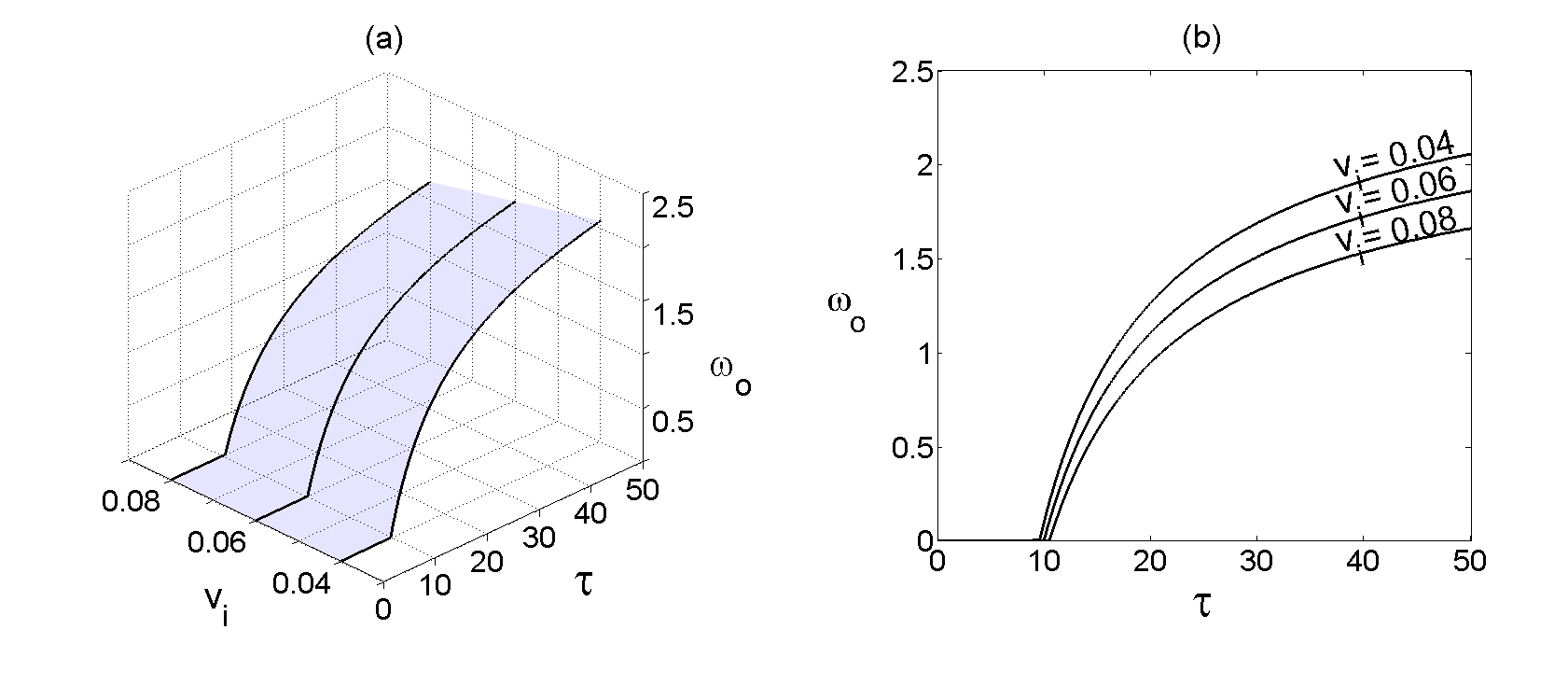
Figure 2: Stability boundaries of the endemic steady state $E^{*}$. The steady state is stable to the left of the surface in (a), and to the left of the lines in (b). Parameter values are $\alpha=0.3,\lambda=0.1,\beta=1.2,r=0.2,\sigma_{s}=0.04,p=0.4,q=0.6,\alpha_{o}=0.2,\lambda_{o}=0.3,\eta=0.05,\delta=0.3,v_{s}=0.06,b=0.4,N=100$.

4 Numerical study of the model

In order to better understand how different parameters affect the stability of the disease-free and endemic equilibria, we use a pseudospectral method [7] implemented in a traceDDE suite in MATLAB to numerically compute characteristic eigenvalues. Figure 1 illustrates how stability of the endemic steady state depends on the disease transmission rate $\beta$, local and global awareness rates $\alpha_{o}$, $\alpha$, $\omega_{o}$, and the time delay $\tau$ of individuals’ response to available information. This figure shows that the endemic equilibrium only exists for a limited range of disease transmission rates, and it is stable for higher rates and unstable for smaller $\beta$. Increasing the awareness rate $\alpha_{o}$ leads to a destabilisation of the endemic steady state, but surprisingly, increasing a global awareness rate $\omega_{o}$ or a local awareness rates $\alpha$ actually results in stabilising an endemic steady state, whilst increasing these rates above certain values makes the endemic steady state unfeasible, in which case the disease-free steady state is stable. In terms of two types of vaccination, naturally, vaccination of aware individuals does not have any noticeable effect on stability of the endemic steady state, whereas increasing the vaccination rate of unaware individuals stabilises the endemic steady state, until it makes $E^{*}$ unfeasible and stabilises the disease-free steady state. Increasing the time delay $\tau$, in accordance with Theorem 3, leads to de-stabilisation of the endemic steady state and the emergence of periodic solutions. Figure 2 further illustrates the stability boundary of the steady state $E^{*}$, showing that for higher vaccination rates, a lower rate of global awareness is required to stabilise the endemic steady state.

Figure 3: Bifurcation analysis of the endemic state: (a) periodic solutions showing the dynamics of $S_{n}$, $S_{a}$, $I$ variables only, (b) amplitude of periodic solutions depending on the time delay $\tau$, (c) period depending on time delay. In each plot, red solid lines correspond to $v_{i}=0.04$, black dashed lines represent $v_{i}=0.06$, and blue dotted lines correspond to $v_{i}=0.08$. Other parameter values are $\alpha=0.3,\lambda=0.1,\beta=1.2,r=0.2,\sigma_{s}=0.04,p=0.4,q=0.6,\omega_{o}=0.1,\alpha_{o}=0.2,\lambda_{o}=0.3,\eta=0.05,\delta=0.3,v_{s}=0.06,b=0.4,N=100$.

Figure 3 demonstrates the results of numerical continuation of the Hopf bifurcation of the endemic steady state, as performed using DDE-BIFTOOL continuation software. It shows that both the amplitude, and the period of periodic solutions increase with the time delay $\tau$, and for higher vaccination rates $v_{i}$ the amplitude of the periodic solution is smaller, while the period is higher.

In Fig. 4 we illustrate how actual dynamics of the system (2) changes depending on system parameters. Figure 4(a) and (b) show the system approaches the stable disease-free or endemic steady states for $R_{v}^{d}<1$ or $R_{v}^{d}>1$, respectively. One should note that according to Theorem 2, the stability of the disease-fee steady state does not depend on the value of the time delay $\tau$, but rather on the basic reproduction number $R_{v}^{d}$ only, so if one keeps the value of $R_{v}^{d}<1$, the same kind of behaviour would be observed for any $\tau>0$. Choosing parameters in the range where $R_{v}^{d}>1$ and increasing the time delays $\tau$ results in the system approaching endemic steady state in an oscillatory manner, with the amplitude of oscillations increasing with the time delay. Once the time delay $\tau$ exceeds the critical value determined by Theorem 3, the endemic steady state becomes unstable, and the system exhibits stable periodic solutions illustrated in Fig. 4(f). The amplitude and period of such solutions themselves depend on the time delay, as has been shown earlier in Fig. 3.

Figure 4: Numerical solutions of the system (2) (a) $\beta=0.6,R_{v}^{d}=0.8977,\tau=0$, (b) - (f) $\beta=1.2,R_{v}^{d}=1.7955$. (b) $\tau=0$, (c) $\tau=4$, (d) $\tau=8$, (e) $\tau=10$, (f) $\tau=16$. Other parameter values are $\alpha=0.3,\lambda=0.1,r=0.2,\sigma_{s}=0.04,p=0.4,q=0.6,\omega_{o}=0.1,\alpha_{o}=0.2,\lambda_{o}=0.3,\eta=0.05,\delta=0.3,v_{s}=0.06,v_{i}=0.04,b=0.4,N=100$.

5 Discussion

This paper has analysed the effects of vaccination and different types of disease awareness on the dynamics of epidemic spread. We have studied analytically and numerically the conditions on system parameters which ensure feasibility and stability of the disease-free and endemic equilibria. These results suggest that stability of the disease-free steady state is independent of the time delay associated with the response of disease-unaware individuals to various types of awareness campaign, but it is rather determined by the basic reproduction number $R_{v}^{d}$ that depends on other epidemiological parameters, as well as awareness rates. On the contrary, stability of the endemic equilibrium does depend on the response time delay in such a way that while the endemic steady state is stable for $\tau=0$ (whenever it is biologically feasible), increasing the time delay can destabilise this endemic steady state and lead to the onset of stable periodic oscillations.

The numerical analysis has provided a number of insights into the relative roles of different parameters, some of which are natural, while others were surprising. Vaccination of aware individuals appears to not have a profound effect on the disease dynamics, while increasing the vaccination rates of unaware individuals (including newborn), can make the endemic steady state unfeasible, so that the disease would be eradicated, and the system would settle on a stable disease-free equilibrium. For large values of the time delay, reducing the rate of the disease transmission destabilises the endemic equilibrium, which should be expected. However, contrary to intuition, the same occurs when one reduces the rates of global awareness or local awareness, whereas one would expect that reduced awareness would support the maintenance of disease in the population, as is the case for the awareness stemming from the reported cases of disease. Moreover, increasing the rates of local and/or global awareness increases the time delay needed to destabilise the endemic steady state. Interestingly, all these different types of disease awareness only affect the stability of the endemic equilibrium for sufficiently large time delay, while for zero and small delays, the endemic steady state is always stable whenever it is feasible, regardless of the rates of awareness.

The results suggest that no matter how efficiently the cases of infection are reported, by itself this is not sufficient to create enough awareness to eradicate an epidemic, whereas global awareness campaign, and increasing the overall awareness level through contacts with other aware individuals are able to achieve this. Furthermore, the analysis shows an important role played by the vaccination of newborns, which can prevent epidemic outbreaks by providing a required level of herd immunity.

When assessing vaccine efficacy, one should be mindful of the fact that a vaccine may not provide complete protection against the disease. There are several approaches to modelling this, such as “all-or-nothing” and “leaky” vaccine scenarios [19, 20, 42]. “All-or-nothing” vaccine is taken to represent a situation, where vaccine works only in some subset of vaccinated individuals, but for them it does provide complete protection. On the other hand, a “leaky” vaccine describes a situation where all vaccinated individuals receive partial protection against the disease. In this paper, we have considered an idealised situation of a vaccine that takes on in all vaccinated individuals and provides complete protection but only for some period of time, i.e. a vaccine with waning immunity. Analysis of the effects of “all-or-nothing” and “leaky” vaccines will be the subject of further research.

References

• [1] A. Abta, H. Laarabi, H.T. Alaoui, The Hopf bifurcation analysis and optimal control of a delayed SIR epidemic model, Int. J. Anal. 2014, 940819 (2014).
• [2] G.O. Agaba, Y.N. Kyrychko, K.B. Blyuss, Time-delayed SIS epidemic model with population awareness, Ecol. Compl. 31, 50-56 (2017).
• [3] G.O. Agaba, Y.N. Kyrychko, K.B. Blyuss, Mathematical model for the impact of awareness on the dynamics of infectious diseases, Math. Biosci. 286, 22-30 (2017).
• [4] R.M. Anderson, R.M. May, Directly transmitted infectious diseases: control by vaccination, Science 215, 1053-1060 (1982).
• [5] J. Arino, K.L. Cooke, P. van den Driessche, J. Velasco-Hernández, An epidemiology model that includes a leaky vaccine with a general waning function, Discr. Cont. Dyn. Syst. B 4, 479-495 (2004).
• [6] H. Bazin, The eradication of smallpox: Edward Jenner and the first and only eradication of a human infectious disease, Academic Press, San Diego (2000).
• [7] D. Breda, S. Maset, R. Vermiglio, Pseudospectral approximation of eigenvalues of derivative operators with non-local boundary conditions, Appl. Num. Math. 56, 318-331 (2006).
• [8] Y.H. Choi, N. Gay, G. Fraser, M. Ramsay, The potential for measles transmission in England, BMC Public Health 8, 338 (2008).
• [9] J. Cui, Y. Sun, H. Zhu, The impact of media on the spreading and control of infectious disease, J. of Dyn. Diff. Eqns. 20, 31-53 (2008).
• [10] J. Cui, X. Tao, H. Zhu, An SIS infection model incorporating media coverage, Rocky Mount. J. Math. 38, 1323-1334 (2008).
• [11] A. d’Onofrio, Stability properties of pulse vaccination strategy in SEIR epidemic model, Math. Biosci. 179, 57-72 (2002).
• [12] P. van den Driessche, J. Watmough, Further notes on the basic reproduction number, in: F. Brauer, P. van den Driessche, J. Wu (Eds.), Mathematical Epidemiology, Springer, Berlin, 159-178 (2008).
• [13] C.P. Farrington, On vaccine efficacy and reproduction numbers, Math. Biosci. 185, 89-109 (2003).
• [14] S. Funk, E. Gilad, C. Watkins, V.A.A. Jansen, The spread of awareness and its impact on epidemic outbreaks, Proc. Natl. Acad. Sci. USA 106, 6872-6877 (2009).
• [15] S. Funk, E. Gilad, V.A.A. Jansen, Endemic disease, awareness, and local behavioural response, J. Theor. Biol. 264, 501-509 (2010).
• [16] S. Funk, M. Salathé, V.A.A. Jansen, V.A.A., Modelling the influence of human behaviour on the spread of infectious diseases: a review, J. Roy. Soc. Interface 7, 1247-1256 (2010).
• [17] D. Greenhalgh, S. Rana, S. Samanta, T. Sardar, S. Bhattacharya, J. Chattopadhyay, Awareness programs control infectious disease - multiple delay induced mathematical model, Appl. Math. Comp. 251, 539-563 (2015).
• [18] T. Gross, B. Blasius, Adaptive coevolutionary networks: a review, J. R. Soc. Interface 5, 259-271 (2008).
• [19] M. Haber, L. Watelet, M.E. Halloran, On individual and population effectiveness of vaccination, Int. J. Epidem. 24, 1249-1260 (1995).
• [20] M.E. Halloran, M. Haber, I.M. Longini, Interpretation and estimation of vaccine efficacy under heterogeneity, Am. J. Epidem. 136, 328-343 (1992).
• [21] V. Hatzopoulos, M. Taylor, P.L. Simon, I.Z. Kiss, Multiple sources and routes of information transmission: implications for epidemic dynamics, Math. Biosci. 231, 197-209 (2011).
• [22] H. Hethcote, The mathematics of infectious diseases, SIAM Rev. 42, 599-653 (2000).
• [23] D. Juher, I.Z. Kiss, J. Saldaña, Analysis of an epidemic model with awareness decay on regular random networks, J. Theor. Biol. 365, 457-468 (2015).
• [24] M. Keeling, M. Tildesley, T. House, L. Danon, The mathematics of vaccination, Math. Today, 40-43 (2013).
• [25] I.Z. Kiss, J. Cassell, M. Recker, P.L. Simon, The impact of information transmission on epidemic outbreaks, Math. Biosci. 225, 1-10 (2010).
• [26] C.M. Kribs-Zaleta, J.X. Velasco-Hernández, A simple vaccination model with multiple endemic states, Math. Biosci. 164, 183-201 (2000).
• [27] H. Laarabi, A. Abta, K. Hattaf, Optimal control of a delayed SIRS epidemic model with vaccination and treatment, Acta Biotheor. 63, 87-97 (2015).
• [28] Y. Li, J. Cui, The effect of constant and pulse vaccination on SIS epidemic models incorporating media coverage, Commun. Nonlin. Sci. Numer. Simulat. 14, 2353-2365 (2009).
• [29] R. Liu, J. Wu, H. Zhu, Media/psychological impact of multiple outbreaks of emerging infectious diseases, Comput. Math. Meth. Med. 8, 153-164 (2007).
• [30] M. Liu, E. Liz, G. Röst, Endemic bubbles generated by delayed behavioral response: global stability and bifurcation switches in an SIS model, SIAM J. Appl. Math. 75, 75-91 (2015).
• [31] P. Manfredi, A. d’Onofrio, A. (Eds.), Modeling the interplay between human behavior and the spread of infectious diseases, Springer, New York (2013).
• [32] X. Meng, L. Chen, B. Wu, A delay SIR epidemic model with pulse vaccination and incubation times, Nonl. Anal. RWA 11, 88-98 (2010).
• [33] A.K. Misra, A. Sharma, J.B. Shukla, Modeling and analysis of effects of awareness programs by media on the spread of infectious diseases, Math. Comp. Mod. 53, 1221-1228 (2011).
• [34] A.K. Misra, A. Sharma, V. Singh, Effect of awareness programs in controlling the prevalence of an epidemic with time delay, J. Biol. Syst. 19, 389-402 (2011).
• [35] A.K. Misra, A. Sharma, J.B. Shukla, Stability analysis and optimal control of an epidemic model with awareness programs by media, BioSystems 138, 53-62 (2015).
• [36] M.A. Penţa, A. Băban, Mass media coverage of HPV vaccination in Romania: a content analysis, Health Edu. Res. 29, 977-992 (2014).
• [37] F.D. Sahneh, C. Scoglio, Epidemic spread in human networks, Proc. IEEE Conf. Decision Control, Orlando, FL, pp. 3008-3013 (2011).
• [38] S. Samanta, S. Rana, A. Sharma, A.K. Misra, J. Chattopadhyay, Effect of awareness programs by media on the epidemic outbreaks: A mathematical model, Appl. Math. Comp. 219, 6965-6977 (2013).
• [39] D. Schenzle, An age-structured model of pre- and post-vaccination measles transmission, IMA J. Math. Appl. Med. Biol. 1, 169-191 (1984).
• [40] M. Sekiguchi, E. Ishiwata, Dynamics of a discretized SIR epidemic model with pulse vaccination and time delay, J. Comp. Appl. Math. 236, 997-1008 (2011).
• [41] A. Sharma, A.K. Misra, Modeling the impact of awareness created by media campaigns on vaccination coverage in a variable population, J. Biol. Syst. 22, 249-270 (2014).
• [42] E. Shim, A.P. Galvani, Distinguishing vaccine efficacy and effectiveness, Vaccine 30, 6700-6705 (2012).
• [43] E. Shim, J.J. Grefenstette, S.M. Albert, B.E. Cakouros, D.S. Burke, A game dynamic model for vaccine skeptics and vaccine believers: measles as an example, J. Theor. Biol. 295, 194-203 (2012).
• [44] B. Shulgin, L. Stone, Z. Agur, Pulse vaccination strategy in the SIR epidemic model, Bull. Math. Biol. 60, 1123-1148 (1998).
• [45] C. Sun, W. Yang, J. Arino, K. Khan, Effect of media-induced social distancing on disease transmission in a two patch setting, Math. Biosci. 230, 87-95 (2011).
• [46] J.M. Tchuenche, N. Dube, C.P. Bhunu, J.R. Smith, C.T. Bauch, The impact of media coverage on the transmission dynamics of human influenza, BMC Pub. Health 11, S5 (2011).
• [47] J.M. Tchuenche, C.T. Bauch, Dynamics of an infectious disease where media coverage influences transmission, ISRN Biomath. 2012, 581274 (2012).
• [48] Y. Wang, J. Cao, Z. Jin, H. Zhang, G. Sun, Impact of media coverage on epidemic spreading in complex networks, Physica A 392, 5824-5835 (2013).
• [49] WHO, Eliminating measles and rubella: Framework for the verification process in the WHO European Region, WHO Regional Office for Europe, Copenhagen, Denmark (2014).
• [50] Q. Wu, X. Fu, M. Small, X.-J. Xu, The impact of awareness on epidemic spreading on networks, Chaos 22, 013101 (2012).
• [51] H. Zhao, Y. Lin, Y. Dai, An SIRS epidemic model incorporating media coverage with time delay, Comp. Math. Meth. Med. 2014, 680743 (2014).
• [52] L. Zuo, M. Liu, Effect of awareness programs on the epidemic outbreaks with time delay, Abstr. Appl. Anal. 2014, 940841 (2014).
• [53] L. Zuo, M. Liu, J. Wang, The impact of awareness programs with recruitment and delay on the spread of an epidemic, Math. Prob. Eng. 2015, 235935 (2015).