Pair creation, motion, and annihilation of topological defects in 2D nematics

Abstract

We present a novel framework for the study of disclinations in two-dimensional active nematic liquid crystals, and topological defects in general. The order tensor formalism is used to calculate exact multi-particle solutions of the linearized static equations inside a uniformly aligned state. Topological charge conservation requires a fixed difference between the number of $q=1/2$ and $q=-1/2$ charges. Starting from a set of hydrodynamic equations, we derive a low-dimensional dynamical system for the parameters of the static solutions, which describes the motion of a half-disclination pair, or of several pairs. Within this formalism, we model defect production and annihilation, as observed in experiments. Our dynamics also provide an estimate for the critical density at which production and annihilation rates are balanced.

I Introduction

Topological defects are non-trivial configurations of a spatially varying order parameter that are associated with localised singularities Mermin (1979). They are topological because these singularities can be classified into distinct groups whose members are related by a homotopy Milnor (1997). The study of topological defects has a long history: they have been widely studied, for example in liquid crystals Gennes and Prost (1993); H et al. (2002) optics Freund (2000); Ilyenkov et al. (2000); Berry and Dennis (2007), and even more recently in biological tissues  Saw et al. (2017); Kawaguchi et al. (2017). In the last few years, there has been a renewed interest from the point of view of topological phase transitions Moore (2010); Wen (2016). Singularities play a crucial role in determining the structure of many physical problems Eggers and Fontelos (2015), and it is therefore a tempting idea to describe the dynamics of the system by the motion of its singularities. This program has been followed extensively in describing the motion of vortices in ideal fluid dynamics Saffman (1992), in the Ginzburg-Landau equation Bethuel et al. (1994), or in Bose-Einstein condensates.

However, many such approaches are based on dilute approximations in which the topological defects are (i) both widely separated from each other and (ii) far from the boundaries Gennes and Prost (1993). The dilute approximation is equivalent to requiring that the deformations induced by each defect to be vanishingly small at the boundaries and in the vicinity of the other defects. If either of these conditions are not satisfied, these problems become much more challenging as defects can no longer be considered independently of each other or the boundaries.

This is because the field surrounding a single defect core is characterized by a singular phase, which cannot in general be matched to either to the field at the boundaries (at infinity) or the field near the cores of the other singularities. In addition, the topology of the space (defined by the Euler characteristic) in which the vector field (e.g. liquid crystalline order) lives imposes constraints on the number and charges of the defects via the Poincaré-Hopf theorem Milnor (1997). For example, a consistent treatment requires one consider multi-particle states with constraints on the number and charge of the defects, such that the total charge adds up to the Euler characteristic (zero for a flat plane with no holes). Recent experiments on active liquid crystals Marchetti et al. (2013) provide a motivation to address these longstanding issues as under many conditions, activity leads to ‘chaotic’ states with a proliferation of defects Sanchez et al. (2012); Sumino et al. (2012); Schaller and Bausch (2013); DeCamp et al. (2015) which consequently are not widely separated from each other or boundaries, requiring one to go beyond the dilute approximation.

In this article we characterize and study the dynamics of topological defects in two-dimensional nematic liquid crystals, though we believe the approach we develop to be more generally applicable to other geometric singularities in a variety of physical systems. To be precise, here we will consider only the lowest energy defects consistent with nematic liquid crystal symmetry, positive and negative half-integer defects or disclinations Gennes and Prost (1993) on a two-dimensional surface. For a plane with no holes, this implies an even number of defects (particles) with equal numbers of positive and negative charges Milnor (1997). Although such particle pairs play an important role in many famous physics problems, such as superconductivity (where positive and negative particles form Cooper pairs), or the Kosterlitz-Thouless transition Kosterlitz and Thouless (1973) (which results from the disassociation of vortex pairs), multi-particle states are usually not known explicitly.

However, in the present paper we find explicit expressions for many-particle states of singularities in nematic liquid crystals, so called disclinations Frank (1958), which have topological charges of $q=\pm 1/2$. This is particularly exciting since we are thus able to mathematically describe the creation of a defect-pair itself, where a pair of oppositely charged particles are formed spontaneously out of a uniform state. Likewise, we characterize the annihilation of pairs of defects, where two particles come together to form a uniform state. We will describe these singular events for an active suspension of elongated particles Sanchez et al. (2012); DeCamp et al. (2015) in a nematic liquid crystal phase. This is an example of active matter driven out of equilibrium by constituents which consume energy, the study of which has emerged recently as an exciting new field in soft condensed matter Marchetti et al. (2013). In the experiment, a thin film of microtubules (MT) is suspended on an oil layer. Molecular motors crosslink MT’s and induce relative sliding, which induces motion, and pumps energy into the fluid layer.

Without activity, the fluid is at rest, and the system relaxes to a uniformly ordered nematic state, in which all particles are oriented in the same direction. However, activity induces a highly non-uniform state, and in particular leads to the creation of a “gas” of defects or disclinations. The random arrangement of defects is due to constant pair-creation and annihilation events. There have been a number of successful large-scale numerical simulations of this system Giomi et al. (2012); Thampi et al. (2013); Wensink et al. (2012); Hemingway et al. (2016), based on a standard continuum model of an active fluid Marchetti et al. (2013). This will serve as a guide for our theoretical calculations.

Previous theoretical attempts at the problem Pismen (2013); Giomi et al. (2014); Shi and Ma (2013) were all based on the hypothetical dynamics of a single defect Pleiner (1988); Ryskin and Kremenetsky (1991). This requires ad-hoc assumptions on the form of the far field, and necessarily introduces a dependence on some length scale, which serves to remove singularities. It is unknown how to identify this length scale uniquely, based on the equations of motion. Our aim here then is therefore to formulate a dynamics for defects based on first principles, relying on the equations of motion only.

II Statics: multi-defect states

Let us begin with a description of the equilibrium states of a uniaxial nematic crystal, described by its director, ${\bf n}=(\cos\theta,\sin\theta)$, for which the Frank-Oseen free energy is Gennes and Prost (1993)

$$F_{\tiny FO}=\frac{K}{2}\int\left|\left|\nabla\mathbf{n}\right|\right|^{2}d{\bf r}=\frac{K}{2}\int\left|\nabla\theta\right|^{2}d{\bf r}\;.$$ (1)

For simplicity, we have used the one-constant approximation $K\equiv K_{1}=K_{2}=K_{3}$. It is crucial to note that in a nematic crystal, ${\bf n}$ is an axial vector, for which ${\bf n}\equiv-{\bf n}$. Similarly, the orientation angle $\theta$ is defined only up to multiples of $\pi$. Points of stationary variation $\delta F_{FO}/\delta\theta=0$ define equilibrium states, solutions of Laplace’s equation

$$\triangle\theta=0\;,$$ (2)

where $\triangle\equiv{\nabla}^{2}$. However, equation (2) does not mean that equilibrium states are defined by a simple linear equation; rather, nonlinearities arise because of the equivalence $\theta\equiv\theta\pm\pi$.

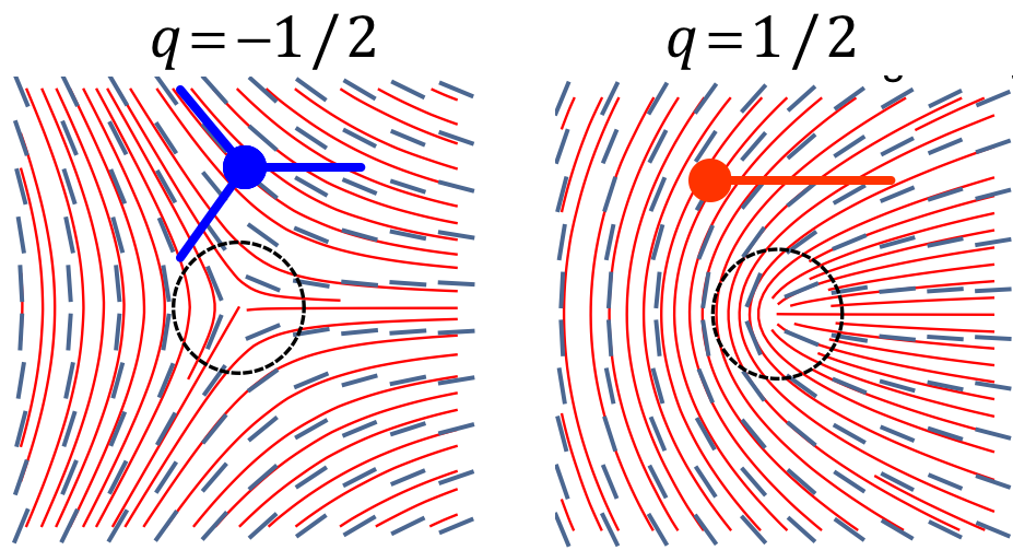
Figure 1: The disclination, equation (3) for $m=\pm 1$, with charge $q=\pm 1/2$.

It was noted by Oseen Oseen (1933); Frank (1958), that equation (2) admits solutions corresponding to the two-dimensional singularities

$$\theta_{d}^{(m/2)}({\bf r})=\frac{m}{2}\phi\;,$$ (3)

where $m$ is an integer and ${\bf r}=r(\cos\phi,\sin\phi)$ is the position vector. The two lowest order disclinations $m=\pm 1$ are shown in Fig. 1. Half-integer values of the prefactor are allowed in equation (3), since $\theta=\pm\pi$ is equivalent to $\theta=0$, so that the director returns to is original state after a full rotation.

Inserting equation (3) back into equation (1), one finds the free energy of a single defect $F^{(q)}=\pi Kq^{2}\ln(L/a)$. To make the result finite, we had to introduce a small scale core size $a$ and a large-scale cutoff $L$. Both scales will be described self-consistently by the theory we are about to develop. However, it does follow from this simple estimate, that in a two-dimensional system the excitations most likely to occur are the two non-trivial lowest energy states $m=\pm 1$.

The topological character of a defect is defined by its topological charge $\displaystyle q=\frac{1}{2\pi}\oint_{\cal C}d\theta=\frac{1}{2\pi}\int_{0}^{2\pi}\frac{d\theta}{d\phi}d\phi\;,\;$where ${\cal C}$ is any closed loop around the defect. Clearly, for the singular solution, equation (3) the result is the charge $q=m/2$, which can take half-integer values. For these half-integer defects, however, there is associated to each defect an attached unbounded singular line at which $\theta$ (equivalently $\bf n$) jumps $\pm\pi$ (the fact that ${\bf n}\equiv-{\bf n}$ means that the singular line is an artefact of the parametrization). This highlights the fact that ${\bf n}({\bf r})$ is insufficient to describe the singularity completely.

In order to rectify this problem, we use an expression for the free energy, due to de Gennes Gennes and Prost (1993), which includes the additional physics necessary to describe the structure of the core of a defect near its center and removes the artificial singular line. The key is to instead of ${\bf n}$, use as order parameter the symmetric, traceless matrix

$$\mathbf{Q}({\bf r})=\left(\begin{array}[]{cc}Q_{1}&Q_{2}\\ Q_{2}&-Q_{1}\end{array}\right)=Q_{0}\left(\begin{array}[]{cc}2n_{x}^{2}-1&2n_{x}n_{y}\\ 2n_{x}n_{y}&1-2n_{x}^{2}\end{array}\right),$$ (4)

which can be expressed in terms of the director ${\bf n}({\bf r})$ and the degree of alignment $Q_{0}({\bf r})$. In particular, the symmetry of ${\bf n}$ is now built into the description. In order to guarantee a smooth solution at the core, we use the Landau-de Gennes free energy

$$F_{LdG}=\int\left(-\frac{A}{2}\left|\mathbf{Q}\right|^{2}+\frac{B}{4}\left|\mathbf{Q}\right|^{4}+\frac{K}{2}\left|\nabla\mathbf{Q}\right|^{2}\right)d{\bf r}\;,$$ (5)

which allows the amount of nematic ordering to vary.

Furthemore, we note that there is no way a single defect can be placed in a neutral environment (for example a constant director ${\bf n}={\bf e}_{x}$) without $\theta$ encountering a singularity. Embedding defects into a system with a uniform director requires that the total charge vanishes, which means there must be an equal number of positive and negative half-charges. Thus in any attempt to construct singular solutions which decay to a uniform director field at infinity, one must automatically contemplate many-particle solutions, which incorporate charge neutrality.

The elementary disclinations $q=\pm 1/2$ now have the local form, $\mathbf{Q}=Q_{0}({\bf r})\left(\begin{array}[]{cc}\cos\phi&\pm\sin\phi\\ \pm\sin\phi&-\cos\phi\end{array}\right),\quad q=\pm\frac{1}{2}\;.$

For ${\bf Q}$ to be smooth near the origin, $Q_{0}(r)$ must go to zero for $r\rightarrow 0$, consistent with its interpretation as a measure of local order: at the center of defect, ${\bf n}$ points in all directions, so there is no order. As a result, zeroes of $Q_{0}({\bf r})=\sqrt{Q_{1}^{2}({\bf r})+Q_{2}^{2}({\bf r})},$ which are places where $Q_{1}({\bf r})$ and $Q_{2}({\bf r})$ vanish simultaneously, are most conveniently used to find the exact position of a disclination. In the following we will now embed the defects into an environment with a uniform director field. From a balance of the first two terms of equation (5), one finds a uniform solution (so that the gradient term disappears) of the form $Q_{1}=\overline{Q}_{0}\cos\xi,\quad Q_{2}=\overline{Q}_{0}\sin\xi\;,\;$where $\xi$ is the (constant) orientation angle and $\overline{Q}_{0}=\sqrt{2A/B}$.

Once more, equilibrium states are found from the vanishing variation of free energy, ${\bf H}=-{\delta F_{LdG}/\delta{\bf Q}}$ which leads to the pair of nonlinear equations

$${\bf H}=0\;{\Rightarrow}\;K\triangle Q_{1,2}+\left[A-2B\left(Q_{1}^{2}+Q_{2}^{2}\right)\right]Q_{1,2}=0\;.$$ (6)

It makes explicit all the nonlinearities contained implicitly in equation (2), and contains additional physics to describe disclinations using smoothly varying fields $Q_{1},Q_{2}$. We are interested in solving equation (6) such that they locally describe a $q=\pm\frac{1}{2}$ disclination yet have a uniform orientation ; without loss of generality we take $\xi=0$, i.e. the nematic is oriented along the $x$-axis.

We linearize equation (6) around the uniform state, which is given by $\overline{Q}_{1}=\overline{Q}_{0}=\sqrt{2A/B}$ and $\overline{Q}_{2}=0$: $Q_{1}=\overline{Q}_{1}+\delta Q_{1},\quad Q_{2}=\delta Q_{2}\;.\;$ Thus the linear equations become

$$\triangle\delta Q_{1}-\kappa^{2}\delta Q_{1}=0,\quad\triangle\delta Q_{2}=0,$$ (7)

where $\kappa=\ell_{Q}^{-1}=\left(2A/K\right)^{1/2}$ is the inverse elastic length scale. This length scale also sets the size of a defect. Linearization of the $\bf Q$ equation makes this problem analytically tractable by assuming variations in $Q_{0}$ are small, but retains all the nonlinearities associated with the variation of the director, $\bf n$. It is an improvement on equation (2) which assumes $Q_{0}$ constant. Once the solution is found in terms of $Q_{1},Q_{2}$, the orientation can be reconstructed by inverting the relations $Q_{1}=Q_{0}\cos 2\theta,\;Q_{2}=Q_{0}\sin 2\theta\;$to find the orientation angle $\theta({\bf r})$.

Now we want so solve equation (7) with boundary condition prescribed at the singularity at the origin; by construction, $\delta Q_{1,2}$ have to vanish at infinity, giving the other required boundary condition. The boundary condition at the singularity is specified by a given angular dependence on a circle of radius $a$ around the origin. The most general ansatz is the Fourier series in $\phi$, $Q_{\alpha}(a,\phi)$ :

$$Q_{\alpha}(a,\phi)=\overline{E}_{\alpha}+\sum_{n=1}^{\infty}\left[\overline{D}_{\alpha}^{(n)}\cos\left(n\phi+\zeta_{\alpha}^{(n)}\right)\right]\;,$$ (8)

where $\alpha=\{1,2\}$. It is here that the topological charge of the imposed defect is fixed, by the lowest non-zero mode $n$ of equation (8). The length $a$ can be interpreted as the core size of the defect, which is a microscopic scale, set by the particle size. It is expected to be much smaller than the elastic length $\kappa^{-1}$, over which elastic stresses relax. A solution to equation (7) for $\delta Q_{\alpha}(r,\phi)$, $\alpha\in\{1,2\}$ is a superposition of Fourier modes of the form Lauga and Stone (2003)

$$\delta Q_{\alpha}=\sum_{n}h_{\alpha,n}(r)\left(A\cos n\phi+B\sin n\phi\right)\;.$$ (9)

Then $h_{1,n}(r)$ are solutions of a modified Bessel equation Gradshteyn and Ryzhik (2014), the solutions which decay at infinity are $K_{n}(\kappa r)=\int_{0}^{\infty}dt\cosh(nt)e^{-\kappa r\cosh t}$. This describes the solution for $r>a$, which is the only part of physical interest. The function $h_{2,n}(r)\sim r^{p(n)}$ is a power law solution of Laplace equation, with $p>0$ for $r<a$ and $p<0$ for $r>a$.

We demonstrate below that only the constant and $n=1$ terms of the Fourier series for the boundary conditions, equation (8) are required to obtain half-integer disclinations and that the free parameters in equations (8) , (9) determine the number, locations and orientations of the defects. Hence restricting our analysis first to only the constant (zero-mode) and the $n=1$ mode (easily generalized to higher modes), we require $Q_{1}(a,\phi)=\overline{E}_{1}+\overline{D}_{1}\cos(\phi+\zeta_{1})\;,\;Q_{2}(a,\phi)=\overline{E}_{2}+\overline{D}_{2}\sin(\phi+\zeta_{2})\;$ on $r=a$. The constant $\overline{E}_{2}$ ($n=0$ term for $Q_{2}$) provides both essential information about the defect topology and a technical difficulty, as it does not correspond to a single term of a sine-Fourier series. In fact it can only be addressed by using an infinite number of terms of the series. To deal with it, we represent it as a sum of Fourier modes, noting the series for a square pulse between $\phi=-\pi$ and $\phi=\pi$ is :

$$\overline{E}_{2}=\frac{4\overline{E}_{2}}{\pi}\sum_{n=0}^{\infty}\frac{(-1)^{n}}{2n+1}\cos\frac{(2n+1)\phi}{2}.$$ (10)

Thus the $n=0$ mode contribution to $\delta Q_{2}({\bf r})$ can be written as a sum of powers $(a/r)^{n+1/2}$, whose coefficients are the terms in the sum equation (10). The resulting expression can be resummed and if we rescale $\delta Q_{1}$ and $\delta Q_{2}$ with $\overline{Q}_{0}$, and write $r$ in units of $a$ (such that $r=1$ at the microscopic size of the defect), we obtain

$$\delta Q_{1}=(E_{1}-1)\frac{K_{0}\left(\Lambda r\right)}{K_{0}\left(\Lambda\right)}+D_{1}\frac{K_{1}\left(\Lambda r\right)}{K_{1}\left(\Lambda\right)}\cos(\phi+\zeta_{1}),$$ (11)

$$\delta Q_{2}=D_{2}\frac{\sin(\phi+\zeta_{2})}{r}+E_{2}f_{2}(r,\phi).$$ (12)

where

$$f_{2}(x,\phi)=\frac{2}{\pi}\left[{\rm arccot}\left(\frac{\sqrt{x}}{\cos\phi/2}+\tan\frac{\phi}{2}\right)+\right.$$

$$\left.{\rm arccot}\left(\frac{\sqrt{x}}{\cos\phi/2}-\tan\frac{\phi}{2}\right)\right].$$

This is one of the main results of this paper.

A couple of examples of typical director configuration are shown in Fig. 2; apart from the imposed $q=1/2$ defect, a second “ghost” defect has appeared, whose position and orientation depends on the parameters chosen. Thus the total charge of the system is zero, and the director field is uniform far away from the pair. Any solution of equation (7) which satisfies uniform boundary conditions must automatically satisfy charge neutrality.

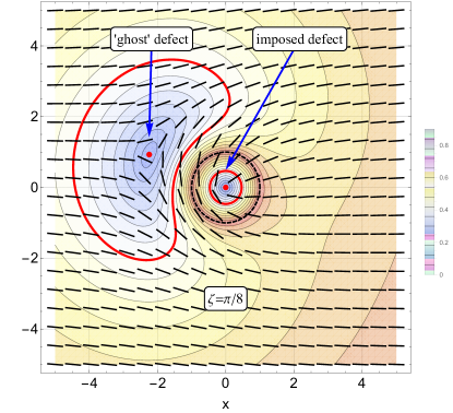
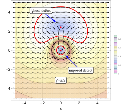
Figure 2: Director configuration (black bars) and order tensor magnitude (contours and colours) for a pair of oppositely charged half-disclinations. The positive defect was imposed in the solution of equation (7), the negative “ghost” emerges to satisfy the constraint of zero charge. Two typical two-defect configurations, as described by equations (11),(12). Here, $D_{1,2}=0.9,E_{1,2}=0,\zeta_{1,2}=\pi/8,\pi/4$

We can thus characterise a pair of defects in terms of 6 scalar parameters $D_{1/2},E_{1/2}$ and $\zeta_{1/2}$. Two examples are illustrated in Fig. 2. Choosing $D>0$ or $D<0$, corresponds to charge $q=1/2$ or $q=-1/2$ for the imposed defect, respectively, and thus effectively interchange the imposed and ghost defects. The angles $\zeta_{1/2}$ control the orientation of the imposed defect relative to the order in the far field. The coefficients $E_{1}$ and $E_{2}$ can be written as $E_{1}=E_{0}\cos\xi$ and $E_{1}=E_{0}\sin\xi$, where $E_{0}$ controls mainly the degree of anisotropy, whereas $\xi$ is the angle between the two orientations. $E_{1}$ and $D$ are the dominant parameters controlling the distance between defects.

To study the defect dynamics, our strategy will be to obtain a reduced model in terms of equations of motion for the parameters, and then to use the time dependent parameter values to calculate the time-dependent vortex configurations once the parameter values have been obtained. Equations (11),(12) correspond to states with at most two defects. However, by including more modes, states with arbitrary number of defects can be generated (see Appendix).

III Defect dynamics: pair creation and annihilation

We study the temporal dynamics of disclinations using the standard equations of nematodynamics at vanishing Reynolds number in two dimensions augmented to include the possibility of additional active stresses Giomi et al. (2012); Marchetti et al. (2013). A key component of these are the Stokes equations describing the motion of a viscous nematic fluid Giomi et al. (2012); Marchetti et al. (2013). They are driven by the active stress ${\boldsymbol{\sigma}}_{a}=\alpha c_{0}^{2}{\bf Q}$, where $c_{0}$ is the concentration of active particles, and the elastic stress, which results from the nematic not being at elastic equilibrium, ${\bf H}\neq 0$, see equation (6). A non-vanishing $\bf H$ indicates an unbalanced elastic stress, so ${\boldsymbol{\sigma}}_{el}=-\lambda Q_{0}{\bf H}+{\bf QH}-{\bf HQ}$. If $\alpha<0$ (“pushers”), the active particles are extensile. The case $\alpha>0$ (“pullers”) corresponds to contractile particles. The so-called alignment parameter $\lambda$ will be discussed below. Both extensile and contractile cases lead generically to instability with increasing $\alpha$, depending on the parameter, $\lambda$. Thus Stokes’ equation for an active incompressible nematic fluid ${\boldsymbol{\nabla}}\cdot{\bf v}=0$ becomes

$$\eta\triangle\mathbf{v}+{\boldsymbol{\nabla}}\cdot\left[{\boldsymbol{\sigma}}_{el}+{\boldsymbol{\sigma}}_{a}\right]=0\;,$$ (13)

To close the system of equations, we need the equation of motion for ${\bf Q}$:

$$\frac{D\mathbf{Q}}{Dt}=\frac{\mathbf{H}}{\gamma}+\lambda Q_{0}\mathbf{V}-\alpha c_{0}(\nabla\cdot\mathbf{Q})\cdot\nabla\mathbf{Q},$$ (14)

where $V_{ij}=(\partial_{i}v_{j}+\partial_{j}v_{i})/2$ and $\omega_{ij}=(\partial_{i}v_{j}-\partial_{j}v_{i})/2$ are the symmetric and antisymmetric parts of the velocity gradient tensor ${\boldsymbol{\nabla}}{\bf v}$, respectively. The corotational derivative $D\mathbf{Q}/Dt=\partial_{t}\mathbf{Q}+\mathbf{v}\cdot{\boldsymbol{\nabla}}\mathbf{Q}+\boldsymbol{\omega}\mathbf{Q}-\mathbf{Q}\boldsymbol{\omega}$ accounts for the fact that rod-like particles move and rotate with the fluid. The first term on the right of equation (4) describes the tendency of the nematic crystal to relax to an elastic equilibrium state, for which ${\bf H}=0$; this occurs on a time scale $\gamma$. The next term describes the motion of an elongated particle in shear flow; the dimensionless parameter $\lambda$ measures the tendency of the particle to align with the flow Edwards and Yeomans (2009). A value of $\lambda=1$ implies total alignment, i.e. particles pointing in the direction of streamlines. Finally, the last term on the right of equation (14) accounts for the tendency of the activity to misalign the nematic, driving it away from equilibrium.

We project the dynamics of ${\bf Q}$, as described by equations (13), (14), onto the space of static solutions found in the previous section. Taking into account all Fourier modes that would be an exact representation. To illustrate the approach with a tractable example, we consider the 6-dimensional space of solutions, equations (11),(12) corresponding to restricting our analysis to the first two modes only. In a first step, we linearize the equations in ${\bf v}$, $\delta Q_{1}$, and $\delta Q_{2}$ to obtain

$$\eta\triangle^{2}\psi=-2\left[\left(\alpha+\lambda\Lambda^{2}\right)+\lambda\triangle\right]\partial_{x}\partial_{y}\delta Q_{1}-\alpha\left[\partial_{x}^{2}-\partial_{y}^{2}\right]\delta Q_{2}$$

$$\quad\quad\quad+\left[(1-\lambda)\partial_{x}^{2}+(1+\lambda)\partial_{y}^{2}\right]\triangle\delta Q_{2}$$ (15)

$$\partial_{t}\delta Q_{1}=\lambda(\partial_{x}\partial_{y}\psi)+\triangle\delta Q_{1}-\Lambda^{2}\ \delta Q_{1}$$ (16)

$$\partial_{t}\delta Q_{2}=2\left[(\lambda+1)\partial_{y}^{2}\psi+(1-\lambda)\partial_{x}^{2}\psi\right]+\triangle\delta Q_{2},$$ (17)

writing the velocity in terms of the stream function $\psi$ Landau and Lifshitz (1984) as ${\bf v}=(\partial_{y}\psi,-\partial_{x}\psi)$.

We expand in the small parameters $\lambda$ and $\alpha$, since for $\lambda=\alpha=0$ the equations of motion reduce to the equilibrium case, with no motion. At each order $\lambda^{n}\alpha^{m}$ in an expansion in the two variables, we can the derive an equation of motion for the coefficients of the equilibrium solutions. First, we expand each of the coefficients into a Taylor series in $\lambda,\alpha$, which results in a corresponding series for $\delta Q_{1/2}$: $\delta Q_{1/2}=\lambda\delta Q_{1/2}^{(\lambda)}+\alpha\delta Q_{1/2}^{(\alpha)}+\ldots\;;\;$ and the stream function $\psi$ can be expanded in the same way. As boundary conditions we impose that $\psi^{(\lambda)}$ vanishes at infinity, and satisfies the no-slip condition $\psi^{(\lambda)}=\partial_{r}\psi^{(\lambda)}=0$ on $r=1$ Happel and Brenner (1983), corresponding to the microscopic defect core. This condition fixes a frame of reference in which the imposed defect is at rest. We perform the expansion to order $\lambda^{2}$ and $\lambda\alpha$ yielding equations of motion for the parameters, $E_{1/2}(t),D_{1/2}(t),\zeta_{1/2}(t)$,

$$\dot{E}_{1}(t)=\left(\bar{\lambda}^{2}+\alpha\bar{\lambda}\right)\frac{1-E_{1}^{(0)}}{4\eta},\quad\dot{E}_{2}=0,$$ (18)

$$\dot{D}_{1}(t)=-\frac{D_{1}^{(0)}}{4\eta}\left[\alpha\bar{\lambda}-\bar{\lambda}^{2}\sec\left(2\zeta_{1}^{(0)}\right)\right]$$ (19)

$$\dot{\zeta}_{1}(t)=\frac{\bar{\lambda}^{2}}{4\eta}\tan\left(2\zeta_{1}^{(0)}\right)$$ (20)

$$\dot{D}_{2}(t)=\frac{D_{1}^{(0)}}{4\eta}\left[-2\bar{\lambda}\cos\left(\zeta_{1}^{(0)}+\zeta_{2}^{(0)}\right)\right.$$

$$\left.+\alpha\sec 2\zeta_{2}^{(0)}\sin\left(\zeta_{1}^{(0)}-\zeta_{2}^{(0)}\right)\right]$$ (21)

$$\dot{\zeta}_{2}(t)=\frac{}{2\eta}\frac{D_{1}^{(0)}}{D_{2}^{(0)}}\left[\bar{\lambda}\sin\left(\zeta_{1}^{(0)}+\zeta_{2}^{(0)}\right)\right.$$

$$\left.-\alpha\sec 2\zeta_{2}^{(0)}\cos\left(\zeta_{1}^{(0)}-\zeta_{2}^{(0)}\right)\right],$$ (22)

whose time-evolution determines the motion of defects, to be described below. $\bar{\lambda}=\Lambda\lambda$ is the rescaled inverse length scale emerging from the interplay of alignment and nematic elasticity. To find the trajectory of defects, one needs to find the position of their cores by finding the regions where nematic order vanishes by solving for $Q_{1}=Q_{2}=0$ at each time step.

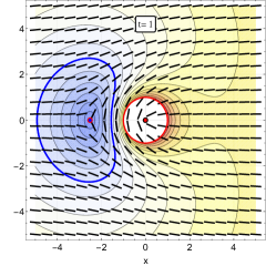
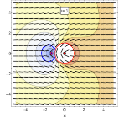
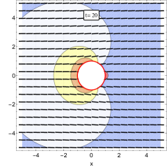
Figure 3: Dynamics of a passive nematic, $\alpha=0$. The three panels show the director and degree of order for $\lambda=0.1$, during the gradual annihilation of the two defects, that relax onto a state with uniform director $\mathbf{n}=\mathbf{e}_{x}.$ I$(D_{1},D_{2}E_{1},E_{2},\zeta_{1},\zeta_{2})^{(0)}=(0.05,0.05,-0.5,0.1,0,0)$ and $\Lambda=10^{-3}$.

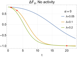
Figure 4: The evolution of the Landau-deGennes free energy function as a function of time is plotted for different values of $\lambda.$ The red points correspond to the three profiles plotted above in Figure 3.

III.1 Passive dynamics

We begin with the dynamics in the absence of activity, $\alpha=0$, an example of which is shown in Fig. 3. The initial condition is chosen that a pair of 1/2 and -1/2 defects is well separated. If only alignment effects are present, which are described by terms proportional to $\lambda$, the systems relaxes to a uniform state. As seen in Fig. 3, the two defects come closer, until they annihilate (the distance between them becomes smaller than the core size) and the orientation becomes uniform.

In Fig.  4, we have also plotted the Landau-deGennes free energy, equation (5) as a function of time, which is seen to decrease monotonically. As a uniform state is reached, the Landau-deGennes free energy approaches a constant value. The relaxation toward the uniform value becomes slower as the alignment parameter decreases.

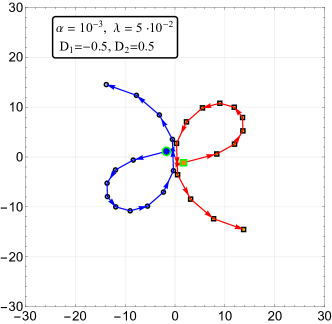
Figure 5: Trajectory of a pair of defects (in the frame of reference of their center of mass) in the presence of low activity, $\alpha=-10^{-3}$, $\lambda=10^{-2}$. Circles represent -1/2 and squares +1/2 defects. As the initial configuration (green, larger markers) evolves, the disclinations trace a spiral, annihilating, then creating a new pair and growing further apart several times.

III.2 Active Dynamics

Next we consider the case where both $\lambda$ and $\alpha$ are nonzero. Finite activity ($\alpha\neq 0$) pumps energy into the system, so we expect defects to be created. On the other hand there is competition with the alignment terms, which cause defects to annihilate. This is indeed seen in Fig. 5, where the two defects are seen with their center of mass at the origin. The initial condition is marked by green squares. At first the two defects move away from one another, but eventually they turn and come closer to one another, and annihilate, as their distance becomes smaller than the core size. However, a new pair is created immediately, starts to move apart, and the process repeats itself. This corresponds very well to what is observed by Sanchez et al. (2012); DeCamp et al. (2015); Wu et al. (2017), where typically annihilation is followed immediately by creation of a new pair. This dynamics are characterised by a rotational component (governed by $\zeta_{1/2}$) and a radial one (governed by the parameters $E_{1}$ and $D_{1}$); as they approach one another or move apart, pair of defects trace spiral-like trajectories (shown in Fig.5).

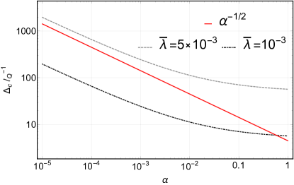
Figure 6: The average separation between defects plotted as a function of activity. The value of $\lambda$ is set to 0.1.

The creation and annihilation of defects will eventually lead to a steady-state density of defects when the creation and annihilation balance out. This implies an average distance between the defect cores, $\Delta$ (the inverse of which determines the density of defects). We estimate this distance by considering a pair of defects at varying initial distances from each other and numerically finding the critical initial distance for which the they neither approach nor repel each other. At small values of $\alpha$, we predict a scaling law $\Delta\propto\alpha^{-1/2}$ which has been observed previously numerically in Hemingway et al. (2016).

It is possible to understand the scaling $\alpha^{-1/2}$ by examining the equations for the dynamics of $Q_{1},$ which is the field that governs the distance between the two defects in a pair. Keeping the terms with lowest order gradients, the equations read

$$\eta\nabla^{4}\psi = -2\left(\alpha+\lambda\Lambda^{2}+\lambda\nabla^{2}\right)\partial_{x}\partial_{y}\delta Q_{1}-\alpha\left(\partial_{x}^{2}-\partial_{y}^{2}\right)\delta Q_{2}$$

$${\normalcolor\partial_{t}\delta Q_{1}}=\lambda(\partial_{x}\partial_{y}\psi)+\nabla^{2}\delta Q_{1}-\Lambda^{2}\ \delta Q_{1}.$$

It is evident that the balance between $-\alpha$, $\lambda\nabla^{2}$ and $\lambda\Lambda^{2}$ in the first equation sets a length scale $\Delta$, defined by

$$\alpha\sim\lambda\left(\frac{1}{\Delta^{2}}+\Lambda^{2}\right)\sim\lambda\left(\frac{1}{\Delta^{2}}+\frac{1}{\ell_{Q}^{2}}\right).$$ (23)

In the regime where $a=1\ll\Delta\ll\ell_{Q},$ this translates into the scaling law

$$\Delta\sim\alpha^{-1/2}\sim\ell_{\alpha},$$

which accounts for the behaviour observed in Fig. 6 for small $\alpha.$ As the active parameter increases, the relative distance between defects becomes comparable to $a=1$, this scaling approximation breaks down (as the distance $\Delta$ plateaus towards $\Delta=a=1).$

IV Discussion

We have formulated a theory for the evolution of the macroscopic structure of a (possibly active) nematic liquid crystal built on a first-principles description of its singularities (topological defects). The dynamics are described principally by the motion of the defects contained in a particular state; however, our equations are for the coefficients of an expansion in modes, and the position of the defects follow as a secondary quantity.

Finally, our model allows for a theoretical prediction of the defect areal density that characterises the chaotic states observed in Sanchez et al. (2012); DeCamp et al. (2015). Our result shows a scaling that agrees with that derived by Hemingway et al. (2016) via numerical simulations of the same equations.

In view of experiments and simulations it would be interesting to describe states with many defects. Although in principle, by adding more modes in our expansion, we can describe states with an arbitrary number of defects, it remains to be seen if this will be practical. An alternative might be to construct superpositions of states made up of pairs of equal and oppositely charged defects, which ensures that these states can be matched to each other without encountering any singularities in the fields.

Most interestingly, the methods we have used can easily be generalised to analyse groups of topological defects that can be found in a variety of field theories whose dynamics can be described by partial differential equations. Natural examples would be vortices in XY-models, polar liquid crystals or Newtonian fluids. Higher charge defects can also be studied simply by specifying the appropriate boundary condition at the imposed defect core. Another interesting direction is the study of populations of defects where the vector field lives on a topologically non-trivial manifold such as a sphere Keber et al. (2014).

Appendix A Appendix: Generating more defects

While the discussion in the manuscript has mainly considered a single non-zero, i.e. $n=1$ mode only, the analysis can be extended to higher modes. As an example, in Fig. 7 we show the evolution of solutions that have three allowed modes $n=1,2$ and 3:

$$\delta Q_{1}=(E_{1}-1)\frac{K_{0}\left(\Lambda r\right)}{K_{0}\left(\Lambda\right)}+D_{1}\frac{K_{1}\left(\Lambda r\right)}{K_{1}\left(\Lambda\right)}\cos(\phi+\zeta_{1})$$ (24)

$$+G_{1}\frac{K_{2}\left(\Lambda r\right)}{K_{2}\left(\Lambda\right)}\cos(2\phi+\zeta_{1})+H_{1}\frac{K_{3}\left(\Lambda r\right)}{K_{3}\left(\Lambda\right)}\cos(3\phi+\zeta_{1})\;,$$

$$\delta Q_{2}=E_{2}f_{2}(r,\phi)+D_{2}\frac{\sin(\phi+\zeta_{2})}{r}$$

$$+G_{2}\frac{\sin(2\phi+\zeta_{2})}{r^{2}}+H_{2}\frac{\sin(3\phi+\zeta_{2})}{r^{3}}\;.$$ (25)

Starting with two defects, (modes $n=2,3$ zero) it shows the bifurcations leading to the production of two more pairs of defects. Our analysis indicates that $n$ defect pairs can be created with $n$ modes.

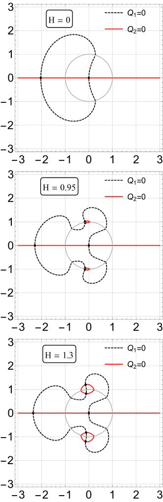
Figure 7: Level lines $Q_{1,2}=0$ (dashed black, solid red respectively) for a solution with three modes. The gray line indicates the core boundary $r=1$. The intersection points (black dots) represent the positions of the topological defects. As the magnitude of the third mode $H$ increases, the level lines change shape and new pairs of defects appear. In the central panel two extra pairs are produced at the interface $r=1$; on the right we see that by varying $H$ the positions of different pairs and of the single disclinations within pairs changes. Here $G_{1,2}=0.1,E_{1,2}=0,\ D_{1,2}=0.9,\ \zeta_{1,2}=0$ and $H_{1,2}=H$ in equations (24), (A).