Observable Gravitational Waves from Higgs Inflation in SUGRA

Abstract:

We consider models of chaotic inflation driven by the real parts of a conjugate pair of Higgs superfields involved in the spontaneous breaking of a grand unification symmetry at a scale assuming its Supersymmetric value. Employing quadratic Kähler potentials with a prominent shift-symmetric part proportional to $c_{-}$ and a tiny violation, proportional to $c_{+}$, included in a logarithm we show that the inflationary observables provide an excellent match to the recent Planck and Bicep2/Keck Array results setting, e.g., $0.012\lesssim c_{+}/c_{-}\lesssim 1/N$ where $-N<0$ is the prefactor of the logarithm. Moreover, we analyze several possible stabilization mechanisms for the non-inflaton accompanying superfield using just quadratic terms. In all cases, inflation can be attained for subplanckian inflaton values with the corresponding effective theories retaining the perturbative unitarity up to the Planck scale.

Published in  PoS EPS-HEP 2017, 047 (2017).

1 Introduction

We focus on the simplest and most promising models of kinetically modified non-minimal Higgs inflation (HI) established in Ref. [1, 2]. Namely, working in the context of Supergravity (SUGRA), we concentrate on the subclass of these models which employ a prominent non-trivial kinetic coupling and only quadratic terms in the adopted Kähler potentials. Moreover, we present novel stabilization functions of the non-inflaton field inspired by Ref. [3]. We below describe the formulation of this type of HI in the context of SUGRA – see Sec. 2 – and then, in Sec. 3, we analyze the inflationary behavior of these models. Our results are exposed in Sec. 4 and our conclusions in Sec. 5.

Throughout the text, the subscript $,\chi$ denotes derivation with respect to (w.r.t) the field $\chi$, charge conjugation is denoted by a star (^∗) and we use units where the reduced Planck scale $m_{\rm P}=2.43\cdot 10^{18}~{}{\mbox{\rm GeV}}$ is set equal to unity.

2 Modeling Higgs Inflation in SUGRA

In Sec. 2.1 we present the basic formulation of a scalar theory within SUGRA and then we outline in Sec. 2.2 our strategy in constructing viable models of HI.

2.1 The General Set-up

Our starting point is the Einstein frame (EF) action for the scalar fields $z^{\alpha}$ within SUGRA [2] which can be written as

$${\sf S}=\int d^{4}x\sqrt{-\widehat{\mathfrak{g}}}\left(-\frac{1}{2}\widehat{{R}}+K_{{\alpha}{\bar{\beta}}}\widehat{g}^{\mu\nu}D_{\mu}z^{\alpha}D_{\nu}z^{*{\bar{\beta}}}-\widehat{V}\right),$$ (1a)

where $$\widehat{{R}} \mathfrak{g} g^{\mu\nu} (+,-,-,-)$$ is the Ricci scalar and is the determinant of the background Friedmann-Robertson-Walker metric, with signature . We adopt also the following notation

$$K_{{\alpha}{\bar{\beta}}}={K_{,z^{\alpha}z^{*{\bar{\beta}}}}}>0\>\>\>\mbox{and}\>\>\>D_{\mu}z^{\alpha}=\partial_{\mu}z^{\alpha}+igA^{\rm a}_{\mu}T^{\rm a}_{{\alpha}{\beta}}z^{\beta}$$ (1b)

are the covariant derivatives for scalar fields $$z^{\alpha} g A^{\rm a}_{\mu} T_{\rm a} z^{\alpha} \widehat{V} K W$$. Here, and henceforth, the scalar components of the various superfields are denoted by the same superfield symbol. Also, is the unified gauge coupling constant, are the vector gauge fields and are the generators of the gauge transformations of . The EF potential, , is given in terms of the Kähler potential, , and the superpotential, , by

$$\widehat{V}=\widehat{V}_{\rm F}+\widehat{V}_{\rm D}\>\>\>\mbox{with}\>\>\>\widehat{V}_{\rm F}=e^{K}\left(K^{{\alpha}{\bar{\beta}}}{\rm F}_{\alpha}{\rm F}^{*}_{\bar{\beta}}-3{|W|^{2}}\right)\>\>\>\mbox{and}\>\>\>\widehat{V}_{\rm D}={1\over 2}g^{2}\sum_{\rm a}{\rm D}_{\rm a}{\rm D}_{\rm a}.$$ (1c)

Here, the summation is applied over the generators $$T_{\rm a}$$ of a considered gauge group – a trivial gauge kinetic function is adopted. Also we use the shorthand

$$K^{{\alpha}{\bar{\beta}}}K_{{\alpha}\bar{\gamma}}=\delta^{\bar{\beta}}_{\bar{\gamma}},\>\>{\rm F}_{\alpha}=W_{,z^{\alpha}}+K_{,z^{\alpha}}W~{}~{}\mbox{and}~{}~{}{\rm D}_{\rm a}=z^{\alpha}\left(T_{\rm a}\right)^{\beta}_{\alpha}K_{\beta}~{}~{}\mbox{with}~{}~{}K_{{\alpha}}={K_{,z^{\alpha}}}.$$ (1d)

In this talk we concentrate on HI driven by $\widehat{V}_{\rm F}$ along a D-flat direction, and therefore the contribution from $\widehat{V}_{\rm D}$ vanishes.

2.2 Inflating With a Superheavy Higgs

The general ideas above can be applied to HI if we employ three chiral superfields, a conjugate pair, $z^{1}=\Phi$ and $z^{2}=\bar{\Phi}$, charged under a local symmetry, e.g. $U(1)_{B-L}$, and a gauge singlet $z^{3}=S$ which play the role of “stabilizer” superfield. We below present the utilized $W$ (Sec. 2.2.1) and $K$’s (Sec. 2.2.2).

2.2.1 Superpotential

Superfields	$S$	$\Phi$	$\bar{\Phi}$
$U(1)_{B-L}$	$0$	$1$	$-1$
$R$	$1$	$0$	$0$

Table 1: Charge assignments of the superfields.

Our scenario is based on the following superpotential

$$W=\lambda S\left(\bar{\Phi}\Phi-M^{2}/4\right)$$ (2)

which is uniquely determined at renormalization level using a $U(1)_{B-L}$ and an $R$ symmetry shown in Table 1. $W$ leads to a $B-L$ phase transition at the scale $M$, which may assume the value predicted by the SUSY unification – see Ref. [2] –, since the SUSY vacuum lies at the direction

$$\langle{S}\rangle=0\>\>\>\mbox{and}\>\>\>|\langle{\Phi}\rangle|=|\langle{\bar{\Phi}}\rangle|=M/2,$$ (3)

and so, $U(1)_{B-L}$ is spontaneously broken. Indeed, the SUSY limit of $\widehat{V}$, after HI, reads

$$V_{\rm SUSY}=\lambda^{2}\left|\bar{\Phi}\Phi-{M^{2}}/4\right|^{2}+\frac{1}{c_{-}(1-Nr_{\pm})}\lambda^{2}|S|^{2}\left(|\Phi|^{2}+|\bar{\Phi}|^{2}\right)+{\rm D-terms},$$ (4)

where $N,c_{-}$ and $r_{\pm}$ are defined below, and it is minimized along the configuration of Eq. (3).

2.2.2 Possible Kähler Potentials

$F_{iS}$	Exponential Form	Logarithmic Form
$F_{1S}$	$\exp\left(-|S|^{2}/N\right)-1$	$-\ln(1+|S|^{2}/N)$
$F_{2S}$	$-N_{S}\left(\exp\left(-|S|^{2}/N_{S}\right)-1\right)$	$N_{S}\ln(1+|S|^{2}/N_{S})$
$F_{3S}$	$-N_{S}\left(\exp\left(-\left(c_{-}F_{-}+|S|^{2}\right)/N_{S}\right)-1\right)$	$N_{S}\ln(1+c_{-}F_{-}/N_{S}+|S|^{2}/N_{S})$

Table 2: Functional forms of $F_{iS}$ with $i=1,2,3$ shown in the definition of $K_{1},K_{2}$ and $K_{3}$ – $N,N_{S}>0$.

The proposed $W$ above may support HI if we combine it with one of the following $K$’s

$$K_{1}=-N\ln\left(1+c_{+}F_{+}+F_{1S}(|S|^{2})\right)+c_{-}F_{-}\,,$$ (5a)

$$K_{2}=-N\ln\left(1+c_{+}F_{+}\right)+c_{-}F_{-}+\ F_{2S}(|S|^{2})\,,$$ (5b)

$$K_{3}=-N\ln\left(1+c_{+}F_{+}\right)+\ F_{3S}(F_{-},|S|^{2})\,,$$ (5c)

where the functions $F_{\pm}=\left|\Phi\pm\bar{\Phi}^{*}\right|^{2}$ assist us in the introduction of shift symmetry for the Higgs fields – cf. Ref. [4] – and the functions $F_{iS}$, given in Table 2, assure the successful stabilization of $S$ along the inflationary path. From the listed $F_{iS}$ only the logarithmic forms for $i=2$ and $3$ are used until now in Ref. [2]. In all $K$’s, $F_{+}$ is included in the argument of a logarithm with coefficient $-N$ whereas $F_{-}$ is outside it. The models can be characterized as completely natural, because, in the limits $c_{+}\rightarrow 0$ and $\lambda\rightarrow 0$, they enjoy the following enhanced symmetries:

$$\bar{\Phi}\rightarrow\ \bar{\Phi}+c^{*},\>\Phi\rightarrow\ \Phi+c\>\>(c\in\mathbb{C})\>\>\>\mbox{and}\>\>\>S\rightarrow\ e^{i\alpha}S\,.$$ (6)

3 Inflation Analysis

We derive the tree-level inflatioanry potential in Sec. 3.1 and then, in Sec. 3.2, we check its robustness against corrections.

3.1 Inflationary Potential

To study accurately enough the inflationary dynamics we use the parametrization

$$\Phi=\phi e^{i\theta}\cos\theta_{\Phi}/{\sqrt{2}}\>\>\>\mbox{and}\>\>\>\bar{\Phi}=\phi e^{i{\bar{\theta}}}\sin\theta_{\Phi}/{\sqrt{2}}\>\>\>\mbox{and}\>\>\>S=({s+i\bar{s}})/{\sqrt{2}}$$ (7)

with $0\leq{\theta_{\Phi}}\leq{\pi}/{2}$. Then, we can show that a D-flat direction is

$$\theta={\bar{\theta}}=s=\bar{s}=0\>\>\>\mbox{and}\>\>\>{\theta_{\Phi}}={\pi/4}.$$ (8)

Along it, the only surviving term of $\widehat{V}_{\rm F}$ for any $K$ in Eqs. (5a) – (5c) is

$$\widehat{V}_{\rm HI}=e^{K}K^{SS^{*}}\,|W_{,S}|^{2}=\frac{\lambda^{2}(\phi^{2}-M^{2})^{2}}{16f_{R}^{2(1+n)}}\>\>\>\mbox{where}\>\>\>f_{R}=1+c_{+}\phi^{2}$$ (9)

plays the role of a non-minimal coupling to gravity. Also, we set

$$n=\left\{\begin{matrix}(N-3)/2\hfill\cr N/2-1\hfill\cr\end{matrix}\right.\>\>\>\mbox{and}\>\>\>K^{SS^{*}}=\left\{\begin{matrix}f_{R}\hfill\cr 1\hfill\cr\end{matrix}\right.\>\>\>\mbox{for}\>\>\>\left\{\begin{matrix}K=K_{1}\hfill\cr K=K_{2}~{}~{}\mbox{or}~{}~{}K_{3}\,.\hfill\cr\end{matrix}\right.$$ (10)

Note that, for $n>0$, $\widehat{V}_{\rm HI}$ develops a local maximum

$$\widehat{V}_{\rm HI}(\phi_{\rm max})={\lambda^{2}n^{2n}(1+n)^{-2(1+n)}/{16c_{+}^{2}}}~{}~{}\mbox{at}~{}~{}\phi_{\rm max}=1/{\sqrt{c_{+}n}}\,.$$ (11)

Consequently, a tuning of the initial conditions is required which can be quantified somehow defining the quantity $\Delta_{\rm max\star}=\left(\phi_{\rm max}-\phi_{\star}\right)/\phi_{\rm max}$, where $\phi_{\star}$ is the value of $\phi$ when the pivot scale $k_{\star}=0.05/{\rm Mpc}$ crosses outside the inflationary horizon.

The EF canonically normalized fields, which are denoted by hat, can be obtained as follows

$$\frac{d\widehat{\phi}}{d\phi}=J,\>\>\widehat{\theta}_{+}=\frac{J\phi\theta_{+}}{\sqrt{2}},\>\>\widehat{\theta}_{-}=\sqrt{\frac{\kappa_{-}}{2}}\phi\theta_{-},\>\>\>\widehat{\theta}_{\Phi}=\phi\sqrt{\kappa_{-}}\left(\theta_{\Phi}-\frac{\pi}{4}\right)\>\>\>\mbox{and}\>\>\>(\widehat{s},\widehat{\bar{s}})=\sqrt{K_{SS^{*}}}(s,\bar{s})\,,$$ (12)

where $J=\sqrt{\kappa_{+}}$ with $\kappa_{+}=c_{-}\left(1+Nr_{\pm}(c_{+}\phi^{2}-1)/{f_{R}}\right)\simeq c_{-}$ and $\kappa_{-}=c_{-}\left(1-{Nr_{\pm}}/{f_{R}}\right)$. Also, $\theta_{\pm}=(\theta\pm\bar{\theta})/\sqrt{2}$. Positivity of $\kappa_{-}$ requires ${r_{\pm}<1/N}$ discriminating a little, thereby, the domains of the solutions with $K=K_{1}$ and $K=K_{2}$ or $K_{3}$. Note that $c_{-}$ influences only $J$ (and not $\widehat{V}_{\rm HI}$).

3.2 Stability and Radiative Corrections

Fields	Einge-	Masses Squared
	states		$K=K_{1}$	$K=K_{2}$	$K=K_{3}$
2 Real	$\widehat{\theta}_{+}$	$\widehat{m}_{\theta+}^{2}$	$6\widehat{H}_{\rm HI}^{2}$		$6(1+1/N_{S})\widehat{H}_{\rm HI}^{2}$
Scalars	$\widehat{\theta}_{\Phi}$	$\widehat{m}_{\theta_{\Phi}}^{2}$	$M^{2}_{BL}+6\widehat{H}_{\rm HI}^{2}$		$M^{2}_{BL}+6(1+1/N_{S})\widehat{H}_{\rm HI}^{2}$
1 Complex Scalar	$\widehat{s},\widehat{\bar{s}}$	$\widehat{m}_{s}^{2}$	$6c_{+}\phi^{2}\widehat{H}_{\rm HI}^{2}/N$	$6\widehat{H}_{\rm HI}^{2}/N_{S}$
1 Gauge Boson	$A_{BL}$	$M_{BL}^{2}$	$g^{2}c_{-}\left(1-Nr_{\pm}/f_{R}\right)\phi^{2}$
$4$ Weyl	$\widehat{\psi}_{\pm}$	$\widehat{m}^{2}_{\psi\pm}$	${6(c_{+}(N-\mathfrak{n})\phi^{2}-2)^{2}\widehat{H}_{\rm HI}^{2}}/{c_{-}\phi^{2}f_{R}^{2}}$
Spinors	$\uplambda_{BL},\widehat{\psi}_{\Phi-}$	$M_{BL}^{2}$	$g^{2}c_{-}\left(1-Nr_{\pm}/f_{R}\right)\phi^{2}$

Table 3: Mass-squared spectrum for $K=K_{1},K_{2}$ and $K_{3}$ along the path in Eq. (2.2) taking $\mathfrak{n}=3~{}[\mathfrak{n}=2]$ for $K=K_{1}$ [$K=K_{2}$ or $K_{3}]$.

To consolidate our inflationary setting we have to check the stability of the trajectory in Eq. (8) with respect to the fluctuations of the non-inflaton fields. Approximate expressions for the relevant mass-squared spectrum are arranged in Table 3. These expressions assist us to appreciate the role of $0<N<6$ [$0<N_{S}<6$] in retaining positive and heavy enough $\widehat{m}^{2}_{s}$ for $K=K_{1}$ [$K=K_{2}$ or $K_{3}$]. Indeed, $\widehat{m}^{2}_{s}\gg\widehat{H}_{\rm HI}^{2}=\widehat{V}_{\rm HI}/3$ for $\phi_{\rm f}\leq\phi\leq\phi_{\star}$ – where $\phi_{\rm f}$ is the value of $\phi$ at the end of HI – as shown in Fig. 1-(a) [Fig. 1-(b)] for $K=K_{1}$ [$K=K_{2}$ or $K_{3}$], $\phi_{\star}=1$ (corresponding to $c_{-}=148$) and $(n,r_{\pm})=(0.042,0.028)$ – see below. From these plots we also infer that the approximate formulas are quite precise for the largest part of the inflationary period. In Table 3 we display also the mass, $M_{BL}$, of the gauge boson $A_{BL}$ – which signals the fact that $U(1)_{B-L}$ is broken during HI – and the masses of the corresponding fermions. Inserting the derived mass spectrum in the well-known Coleman-Weinberg formula, we can find the one-loop radiative corrections, $\Delta\widehat{V}_{\rm HI}$ to $\widehat{V}_{\rm HI}$. It can be verified that our results are immune from $\Delta\widehat{V}_{\rm HI}$, provided that the renormalization group mass scale $\Lambda$, is determined conveniently – see Ref. [4].

4 Results

The free parameters of our setting are $n,r_{\pm}=c_{+}/c_{-}$ and $\lambda/c_{-}$ since if we perform the rescalings $\Phi\rightarrow\Phi/\sqrt{c_{-}}~{}~{}~{}\mbox{and}~{}~{}~{}\bar{\Phi}\rightarrow\bar{\Phi}/\sqrt{c_{-}}$ we see that $W$ depends on $\lambda/c_{-}$ and $K$ on $n$ and $r_{\pm}$. In Sec. 4.1 we confront the models with the observations and in Sec. 4.2 we show that these do not face any problem with the perturbative unitarity.

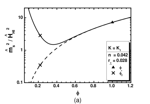
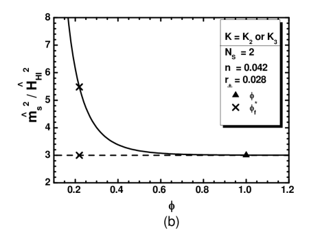
Figure 1: The ratio $\widehat{m}^{2}_{s}/\widehat{H}_{\rm HI}^{2}$ as a function of $\phi$ for $\phi_{\star}=1$ and $(n,r_{\pm})=(0.042,0.028)$ computed by the exact numerical (solid line) or the approximate analytic (dashed line) formulas. We set (a) $K=K_{1}$ and (b) $K=K_{2}$ or $K_{3}$ with $N_{S}=2$. The values corresponding to $\phi_{\star}$ and $\phi_{\rm f}$ are also depicted.

4.1 Testing Against Observations

To compare the predictions of our models with the observations, we first compute – applying standard formulas – the number, ${\widehat{N}_{\star}}$, of e-foldings that the scale $k_{\star}$ experiences during HI and the amplitude, $A_{\rm s}$, of the power spectrum of the curvature perturbations generated by $\phi$ for $\phi=\phi_{\star}$. These observables must be compatible with the requirements [5], i.e., ${\widehat{N}_{\star}}\simeq 58$ and $\sqrt{A_{\rm s}}\simeq 4.627\cdot 10^{-5}$ which assist us in deriving $\phi_{\star}$ and $\lambda/c_{-}$ as functions of $n$ and $r_{\pm}$. We then extract the spectral index, $n_{\rm s}$, its running, $a_{\rm s}$, and the tensor-to-scalar ratio, $r$. These must be in agreement with the fitting of the Planck, Baryon Acoustic Oscillations (BAO) and Bicep2/Keck Array data (BK14) [5, 6] with $\Lambda$CDM$+r$ model, depicted by gray and dark gray contours in Fig. 2-(a). The various lines represent the theoretically allowed values for $K=K_{2}$ or $K_{3}$ and various $n$’s as shown in the legend. The variation of $r_{\pm}$ is shown along each line. For low enough $r_{\pm}$’s – i.e. $r_{\pm}\leq 0.0005$ – the various lines converge to $(n_{\rm s},r_{0.002})\simeq(0.947,0.28)$ obtained within quatric inflation defined for $c_{+}=0$. Increasing $r_{\pm}$ the various lines enter the observationally allowed regions and cover them allowing us to define a minimal and maximal $r_{\pm}$ corresponding to a maximal and minimal $r$ respectively. The lines with $n>0$ [$n<0$] cover the left lower [right upper] corner of the allowed range. In conclusion, the observationally favored region can be wholly filled varying conveniently $n$ and $r_{\pm}$.

Varying continuously these parameters, we delineate the allowed region of our models in Fig. 2-(b). The conventions adopted for the various boundaries are shown in the legend of the plot. In particular, we take into account [5] the upper bound $r\leq 0.07$ and the lower bound $n_{\rm s}\geq 0.959$. Fixing $n_{\rm s}$ to its central value we obtain the thick solid line along which we get clear predictions for $(n,r_{\pm})$ and the remaining inflationary observables. Namely, for $n_{\rm s}=0.968$ and ${\widehat{N}_{\star}}\simeq 58$, we find

$$-1.21\lesssim{n\over 0.1}\lesssim 0.215,\>\>\>0.12\lesssim{r_{\pm}\over 0.1}\lesssim 5,\>\>\>0.4\lesssim{r\over 0.01}\lesssim 7\>\>\>\mbox{and}\>\>\>0.25\lesssim 10^{5}{\lambda\over c_{-}}\lesssim 2.6\,.$$ (13)

The utilized in Fig. 1 values $(n,r_{\pm})=(0.042,0.025)$ yields the central values of observables, i.e., $(n_{\rm s},r)=(0.968,0.028)$. Hilltop HI is attained for $0<n\leq 0.0215$ and there, we get $\Delta_{\rm max\star}\gtrsim 0.4$. The relevant tuning is therefore very mild. The parameter $a_{\rm s}$ is confined in the range $-(5-6)\cdot 10^{-4}$ and so, our models are consistent with the fitting of data with the $\Lambda$CDM+$r$ model [5]. Obviously, our models are testable by the forthcoming experiments – e.g., Core$+$, LiteBird, Bicep3/Keck Array and SPIDER [7] – searching for primordial gravity waves since $r\gtrsim 0.0019$.

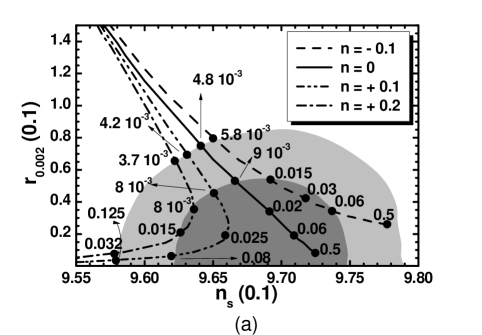
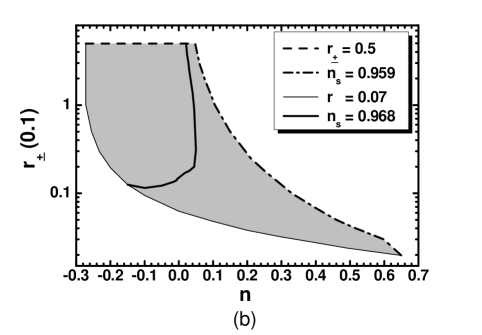
Figure 2: (a) Allowed curves in the $n_{\rm s}-r_{0.002}$ plane for $n=-0.1,0,0.1,0.2$ with the $r_{\pm}$ values indicated on the curves – the marginalized joint $68\%$ [$95\%$] regions from Planck, BAO and BK14 data are depicted by the dark [light] shaded contours. (b) Allowed (shaded) regions in the $n-r_{\pm}$ plane. In both graphs we use $K=K_{2}$ or $K_{3}$ with $N_{S}=2$. The conventions adopted for the various lines are shown.

4.2 Perturbative Unitarity

As can be seen numerically, there is a relatively large lower bound on $c_{-}$ for every $r_{\pm}$ above which $\phi_{\star}\leq 1$. This fact stabilizes our proposal against corrections from higher order terms of the form $(\Phi\bar{\Phi})^{p}$ with $p>1$ in $W$ – see Eq. (2). Moreover, this fact does not jeopardize the validity of the corresponding effective theory since these respect perturbative unitarity up to $m_{\rm P}=1$ as can be inferred by analyzing the small-field behavior of our models. To this end, we expand about $\langle{\phi}\rangle=M\ll 1$ in terms of $\widehat{\phi}$ the second term in the right hand side of Eq. (1a) for $\mu=\nu=0$ and $\widehat{V}_{\rm HI}$ in Eq. (9). Our results can be written as

$$J^{2}\dot{\phi}^{2}\simeq\left(1+3Nr_{\pm}^{2}\widehat{\phi}^{2}-5Nr_{\pm}^{3}\widehat{\phi}^{4}+\cdots\right)\dot{}\widehat{\phi}^{2}\>\>\>\mbox{and}\>\>\>\widehat{V}_{\rm HI}\simeq\frac{\lambda^{2}\widehat{\phi}^{4}}{16c_{-}^{2}}\left(1-2(1+n)r_{\pm}\widehat{\phi}^{2}+\cdots\right)\,.$$ (14)

From the expressions above we conclude that our models are unitarity safe up to $m_{\rm P}$ since $r_{\pm}\leq 1/N$ as shown below Eq. (12).

5 Conclusions

We reviewed the implementation of kinetically modified non-minimal HI in the context of SUGRA. The models are tied to the super-and Kähler potentials given in Eqs. (2) and (5a) – (5c). Prominent in this setting is the role of a softly broken shift-symmetry whose violation is parameterized by the quantity $r_{\pm}=c_{+}/c_{-}$. Variation of $r_{\pm}$ in the range $(0.012-1/N)$ together with the variation of $n$ – defined in Eq. (10) – in the range $(-0.121-0.0215)$ assists in fitting excellently the present observational data and obtain $r$’s which may be tested in the near future. These inflationary solutions can be attained even with subplanckian values of the inflaton requiring large $c_{-}$’s and without causing any problem with the perturbative unitarity.