Mobile IMUs Reveal Driver’s Identity From Vehicle Turns

Abstract

As vehicle maneuver data becomes abundant for assisted or autonomous driving, their implication of privacy invasion/leakage has become an increasing concern. In particular, the surface for fingerprinting a driver will expand significantly if the driver’s identity can be linked with the data collected from his mobile or wearable devices which are widely deployed world-wide and have increasing sensing capabilities.

In line with this trend, this paper investigates a fast emerging driving data source that has driver’s privacy implications. We first show that such privacy threats can be materialized via any mobile device with IMUs (e.g., gyroscope and accelerometer). We then present Dri-Fi (Driver Fingerprint), a driving data analytic engine that can fingerprint the driver with vehicle turn(s). Dri-Fi achieves this based on IMUs data taken only during the vehicle’s turn(s). Such an approach expands the attack surface significantly compared to existing driver fingerprinting schemes. From this data, Dri-Fi extracts three new features — acceleration along the end-of-turn axis, its deviation, and the deviation of the yaw rate — and exploits them to identify the driver. Our extensive evaluation shows that an adversary equipped with Dri-Fi can correctly fingerprint the driver within just one turn with 74.1%, 83.5%, and 90.8% accuracy across 12, 8, and 5 drivers — typical of an immediate family or close-friends circle — respectively. Moreover, with measurements on more than one turn, the adversary can achieve up to 95.3%, 95.4%, and 96.6% accuracy across 12, 8, and 5 drivers, respectively.

I Introduction

As data of vehicle maneuver becomes abundant for assisted or autonomous driving, their implication of privacy invasion/leakage has become an increasing concern. To prevent potential privacy violations, the U.S. Congress has enacted a law for enforcing driving data privacy in Dec. 2015 [1]. In particular, the law forbids disclosure of personally identifiable information of the owner or the lessee of the vehicle. In Dec. 2016, NHTSA also enforced the protection of any data that can be “reasonably linkable” to driver identification [2].

Despite these legislations, researchers have demonstrated that driver’s privacy can indeed be breached by accessing in-vehicle data through an On-Board Diagnostics (OBD-II) dongle. For example, the authors of [3, 4] showed that the driver’s identity can be revealed by analyzing the vehicle’s Controller Area Network (CAN) data collected through the OBD-II port. Although this could be a severe privacy threat, its practicability/feasibility has been questioned for two reasons. First, due to security concerns, car manufacturers are beginning to restrict the OBD-II port access, i.e., allowing its access only during diagnostics (while the vehicle is parked) [5]. Second, even with OBD-II access, existing driver-fingerprinting schemes require a time-consuming task of reverse engineering in-vehicle data [6, 7]. All of these together make it very difficult to invade the driver’s privacy via the OBD-II port.

Due to the nature of in-vehicle data being obscure and difficult to access (e.g., physical access to one’s car), researchers/developers increasingly use IMUs — available on various devices such as smartphones, OEM-authorized OBD-II dongles, and wearables — as an alternative source of driving data for enhancing driving experience and safety. This use of IMUs in the automotive ecosystem has led to the development of various “beneficial” (c.f. malicious) applications such as driving-assistance systems [8], adjustable auto insurance [9], and fuel-efficient navigations.

Collection and exploitation of IMU data also create concerns of breaching drivers’ privacy. In particular, data-collection entities might be able to infer the driver’s identity from the collected IMU data, leading to an incontrovertible breach of the driver’s privacy. This paper focuses on the driver’s identity privacy, and hence questions “Would existing schemes on mobile devices breach the driver’s privacy? Can an adversary with access to only IMU data achieve it?”

On one hand, researchers have shown that one’s privacy can be breached if his/her device is identified/tracked via stealthy identifiers available on the device. For example, by leveraging the imperfection of IMU components [10, 11] or non-cookie web tracking techniques (e.g., supercookies [12]) on a mobile device, an adversary can identify the device and/or its user. On the other hand, instead of identifying the device itself (and hence its owner), other existing schemes attempt to identify the user through his/her behavior or interaction with the device (e.g., touch screen behavior [13], DNS traffic pattern [14]). Although these existing schemes indeed breach privacy of the device owner/user, they do not necessarily breach the actual driver’s privacy. For example, suppose driving data was collected from a smartphone while its owner was in a car as a passenger. In such a case, the collected data did not originate from the actual driver’s device, and hence will not help identify the driver. Similarly, existing schemes cannot identify the driver when someone simply takes his phone and then goes on for a drive. Meanwhile, an interesting but yet unanswered question is “if an adversary reads and analyzes the IMU data in more depth, would the consequences be different?” Behind the paradigm shift of how devices (equipped with IMUs) are being used/integrated in contemporary automotive ecosystems (e.g., vehicle authentication via smartphones, event data recording via IMUs), there could exist many uncovered scenarios where the driver’s privacy could be unintentionally breached.

In this paper, we propose a new driver fingerprinting scheme called Dri-Fi (Driver Fingerprint), which can be used by an adversary to stealthily infer the driver’s identity based on the readings of zero-permission mobile IMUs, i.e., gyroscope, accelerometer, and magnetometer. By developing and using Dri-Fi, we focus on the risk of breaching the driver’s privacy based on driving data that is far more easily obtainable and accessible than in-vehicle data, i.e., IMU data.

The key challenge for Dri-Fi to fingerprint drivers is that it has much less information available than the existing schemes that use in-vehicle data [3, 4]; all Dri-Fi has is access to IMU sensor readings. Dri-Fi overcomes this challenge by constructing a driving behavior profile based on the drivers’ turning maneuver — a common yet representative maneuver. There are two reasons for using vehicle “turns” to represent the driver’s behavior: 1) turns are behavior-rich actions that reflect how the driver accelerates/decelerates, and at the same time, how s/he steers, and 2) turns are less likely to be affected by traffic conditions than other maneuvers. For example, deceleration can be affected greatly by the frontal car whereas turns are not. So, once Dri-Fi detects a turn, it derives three new features: 1) the acceleration along the end-of-turn axis, which is defined as the axis orthogonal to the vehicle’s direction when the turn started, 2) the deviation in the first feature, and 3) the deviation in the yaw rate. These features function as the cornerstone of Dri-Fi’s driver fingerprinting as they reflect the driver’s unique behavior — they are only affected by how the driver actually turns the steering wheel or how s/he presses the acceleration/brake pedal while making a turn. Our extensive experimental evaluation will later show that these features vary only with drivers, but not with car models or trip routes. Once these three features are derived for a detected turn, Dri-Fi computes various percentiles and their autocorrelations which are then used to construct the feature vector for machine classifiers, such as Naive Bayes, SVM, and Random Forest. Dri-Fi can, therefore, fingerprint the driver with a high probability, even when s/he makes just one left/right turn. As more turns are made by the driver within a trip, Dri-Fi exploits such accumulated information for driver fingerprinting to reduce false positives/negatives, enhancing its accuracy. In addition to the driver fingerprinting, we also discuss how an adversary may utilize its IMU measurements to construct a well-formulated training dataset from scratch, which is essential for the underlying machine classifiers. Note that all existing studies (had to) assume the training dataset, which has the correct labels of all targeted drivers, was given to the adversary, which may not hold in practice.

We evaluated Dri-Fi extensively by collecting IMU data from a smartphone while 12 different drivers (9 males, 3 females) were driving either around the campus or in an urban/rural area. Our results have shown that by using Dri-Fi, the driver can be identified within one left/right turn, with accuracies of 74.1%, 83.5%, and 90.8% across 12, 8, and 5 drivers respectively. Dri-Fi’s achievement of high accuracy with just one turn implies a severe driver privacy invasion. Also, Dri-Fi’s performance is in sharp contrast to existing studies that require several minutes of measurements from tens of in-car sensors. As the driver made 8 turns, Dri-Fi was able to achieve accuracies of 95.3%, 95.4%, and 96.6% across 12, 8, and 5 drivers, respectively.

This paper makes the following main contributions:

• Discovery of three new features which are shown to be distinct between different drivers and independent of vehicles and trip routes (Sec. III);

• Development of Dri-Fi, which extracts the new features when the driver makes a left/right turn, and thus achieves driver fingerprinting (as soon as the driver makes a turn) with high accuracy (Sec. III);

• Implementation and extensive evaluation of Dri-Fi using commodity smartphones (Sec. IV).

II Motivation, Adversary Model, and Goal

Although the abundance of driving-related data has brought various benefits to our lives, their availability can also breach the driver’s privacy.

II-A Why Not Fingerprinting Drivers with In-car Data?

An adversary with access to sensors on an in-vehicle network, such as the Controller Area Network (CAN), can fingerprint the driver [3, 4, 15, 16, 17]. (Such schemes will be detailed in Sec. V.) Despite the rich and low-noise in-car data for the adversary to fingerprint drivers, s/he must meet the following two minimum requirements to acquire the data, which are assumed to have been met in all existing studies.

Access to In-car Data. To read and extract values of sensors on an in-vehicle network, the adversary must have access to the sensors data. To gain such an access, s/he may either 1) remotely compromise an Electronic Control Unit (ECU), or 2) have a compromised OBD-II dongle plugged in the victim’s vehicle in order to read in-car data. For the first case, however, depending on the ECU that the adversary compromised, s/he may not be able to read all sensors data of interest, mainly because the ECUs which produce those data may reside in different in-vehicle networks (e.g., some on high-speed CAN and others on low-speed CAN). For the second case, the adversary has indeed control of a plugged-in and compromised OBD-II dongle, and therefore, in contrast to a compromised ECU, is likely to have access to all sensors data of interest (as shown in [3, 17]). However, for security reasons, car manufacturers are increasingly blocking/restricting in-car data access through the OBD-II port except when the vehicle is parked [5]. Thus, the adversary will less likely be able to access in-car data.

Reverse-engineering Messages. Even when the adversary has access to in-vehicle network messages, s/he must still (i) understand where and in which message the sensor data (of interest) is contained, and (ii) translate them into actual sensor values (e.g., transformation coefficients for addition/multiplication of raw sensor data [3]). In-vehicle network messages are encoded by the vehicle manufacturers and the “decoding book,” which allows one to translate the raw data is proprietary to them. Therefore, unless the adversary has access to such a translator, s/he would have to reverse-engineer the messages, which is often painstaking and incomplete.

Although the adversary may have abundant resources to fingerprint the driver, meeting the above two requirements may be difficult or even not possible.

II-B Adversary Model

Due to the difficulty and (even) impracticality of an adversary fingerprinting the driver via in-vehicle (CAN-bus) data, we consider the following adversary who might fingerprint the driver without the difficulties of state-of-the-art solutions. In particular, we consider the adversary with a data-collection entity that aims to fingerprint the driver based on zero-permission mobile IMU data. We assume that the adversary has access to the target’s mobile IMU data while s/he was driving. As mobile IMUs are available in various commodity mobile/wearable devices such as smartphones, watches, and even in OBD-II dongles, the adversary can compromise one of them (belonging to the target), and obtain the required IMU data for driver fingerprinting. This means that the adversary would have a much larger attack surface than existing driver fingerprinting schemes. One example of such an adversary would be a smartphone malware programmer who builds an app to stealthily collect the target’s IMU data. Another example could be a car insurance company that might reveal information other than what was initially agreed on via the collected/stored IMU data available on its OBD-II dongles.

II-C Motivating Scenarios

Integrating mobile IMU sensors with the automotive ecosystem can, on one hand, lead to development of numerous beneficial apps. On the other hand, it may violate the driver’s privacy. In what follows, we state three double-edged-sword scenarios, which at first glance seem beneficial for our daily driving experience but could lead to a severe privacy violation; in fact, more severe than what has already been studied/uncovered.

II-C1 Vehicle Authentication

To enable a more convenient car-sharing experience, car companies, such as Volvo [19] and Tesla [20], started to let car owners unlock and start their cars (e.g. new Tesla model 3) by using their smartphone apps, thus replacing a key fob with a smartphone. By installing this authorized app, the car owner first designates eligible drivers as a whitelist. All allowed drivers can then unlock and start the car with authentication through the Bluetooth link between the car and their smartphones.

Privacy violation case. Alice owns a car with this functionality. Her husband Bob’s driver’s license was suspended. So, Alice is unable to register him as a driver in the whitelist, due to a background check conducted by the car company. One day, Alice asks Bob to drive the car for some reasons. To evade the driver authentication, Alice temporarily gives Bob her phone to drive the car. However, if the car company’s app had stored IMU data and thus had the driving profiles of all whitelisted drivers, with the capability of identifying the driver from IMU data, the car company can determine that the current driving pattern (which is Bob’s) does not match with any of the whitelisted. This becomes a definite privacy violation if the car company had initially stated/claimed that all the IMU data (while driving) reveals how the car moves, not who actually drives it. However, the driver’s identity can be found via in-depth analysis.

II-C2 Named Driver Exclusion

Many states in the U.S. permit “named driver exclusion” to allow auto insurance buyers to reduce their premium [21, 22]. Under this plan, the insurance company will not accept any excuses for allowing the excluded person to drive. Therefore, Department of Motor Vehicles (DMV) specifically warns all drivers of the fact that, to avoid driving without any insurance coverage, the excluded individuals should not drive the insuree’s car [23].

Privacy violation case. Suppose Bob’s wife, Alice, is a legitimate driver. However, to reduce the cost of their family insurance plan, Bob excludes Alice from the plan. Bob’s smartphone has installed the insurance company’s app, which not only manages his insurance account but also keeps record of the driving IMU data as an Event Data Recorder (EDR). One night, Bob was in a bad physical condition and hence asked Alice to drive him home. Unfortunately, they ran into an incident. At the court, the insurance company defended itself by showing the driving IMU data — measured during that night when the accident occurred — matched Alice’s, not Bob’s, driving profile. Thus, the company refused to reimburse Bob and won the lawsuit. Note that the initial purpose of EDR functionality on the app was not for driver fingerprinting but for recording events, an undetermined privacy violation.

II-C3 Utilization of IMU Data

Unlike conventional OBD-II dongles (designed for diagnostics), car manufacturers are designing and developing a new type of dongle, which does not provide users with raw CAN data but provides them in a “translated” format (e.g., JSON format). Ford OpenXC [24] and Intel-based OBD-II dongles [25] are examples of such a design. This way, the car OEMs’ plugged-in dongle reads and translates metrics from the car’s internal network and provides them to the user without revealing proprietary information. Thus, while providing the necessary information to the users, car OEMs can let them install vehicle-aware apps which have better interfaces based on a context that can minimize distraction while driving [24].

Privacy violation case. Alice has the car OEM’s dongle, which provides her the translated CAN data, plugged in her car so that she can gain more insight into her car operation. Due to a security breach on the dongle, suppose Mallory has access to the data being read from the dongle, but only in a translated format. Note that even with access to raw CAN data, Mallory would still need to reverse engineer the messages; we are relaxing the technical requirements for Mallory. He may fail because the translated data that Mallory has access might not contain the required information for in-car-data-based driver fingerprinting. Note that the most significant feature used for driver fingerprinting in [3] was the brake pedal position, which unfortunately is not provided by the Ford OpenXC [24]. However, since those dongles are always equipped with IMUs for data calibration, Mallory uses his malware to read the IMUs instead, and thus attempts to identify the driver. This implies that Mallory might not even need to access the translated data at all, thus lowering the technical barrier for the adversary. Through security by obscurity, the translation of data itself might provide some sort of privacy. However, the IMUs installed on those dongles, designed for calibration, might ironically threaten the driver’s privacy.

II-D Our Goal

To breach the driver’s privacy, the adversary needs an efficient way of fingerprinting the driver solely based on IMU data. Researchers have already demonstrated the feasibility of an adversary breaching the driver’s privacy by fingerprinting him/her with in-car data. We refer to such an adversary as a high-resource adversary due to his/her access to the rich and low-noise in-car data. However, we still do not know if a low-resource adversary, with access to only the target’s IMU data, can fingerprint the driver; it may even be infeasible due to his/her insufficient resource(s). Therefore, our goal is to shed light on an unexplored but important question: “Within a short duration, can a low-resource adversary fingerprint the driver, i.e., having access to only IMUs?”

III System Design

We propose Dri-Fi, which acquires IMU sensor measurements from the victim/target driver and exploits them for identifying the driver.

III-A Overview of Dri-Fi

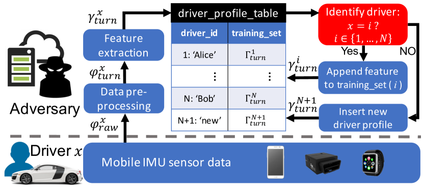
Figure 1: System overview of Dri-Fi.

Fig. 1 presents a high-level overview of Dri-Fi as a 4-step process where the adversary acquires the required raw IMU sensor data $\varphi^{x}_{raw}$ for fingerprinting driver $x$. The data can be acquired either at the end of, or periodically during a trip. First, Dri-Fi pre-processes $\varphi^{x}_{raw}$ to remove noises and extracts the sensor measurements only while $x$ was making a (left/right) turn (Sections III-B–III-C). So, it obtains $\varphi^{x}_{turn}$. Next, based on the thus-obtained $\varphi^{x}_{turn}$, Dri-Fi constructs a set of features, i.e., a feature vector $\gamma^{x}_{turn}$. Then, based on a Gaussian Mixture Model (GMM) (to be detailed in Section III-F), the adversary first verifies whether $\gamma^{x}_{turn}$ closely matches any of his/her previously obtained training data $\Gamma^{n}_{turn}$ in the driver_profile_table, where $n\in\{1,\ldots,N\}$ and $N$ is the number of drivers the adversary had learned about. If there is a close match, s/he exploits $\gamma^{x}_{turn}$ as an input for machine classifiers with the training set as driver_profile_table. As a result, s/he identifies the driver $x$ to be $i\in\{1,\ldots,N\}$ (Sections III-D–III-E). Finally, s/he appends $\gamma^{x}_{turn}$ to his/her driver_profile_table with label $i$. Meanwhile, based on GMM, if $\gamma^{x}_{turn}$ does not closely match any of those in the driver_profile_table, s/he constructs a new driver training dataset for driver $x$.

Note that the adversary needs to have driver_profile_table constructed before identifying driver $x$. Due to this requirement, existing driver fingerprinting schemes with CAN data assume that the adversary already has a complete training set for all the targeted drivers. However, this assumption is difficult to be met in practice. In the following sections, to focus on the design and discussion of Dri-Fi, for now, we assume that the adversary does have the complete training set; the same assumption as in previous studies. We will present in Section III-F how such an assumption can be relaxed by using our context-based approach for constructing the training set from scratch.

III-B Data Collection and Pre-processing

Dri-Fi continuously collects the raw IMU data $\varphi_{raw}=\{gyro_{raw},acc_{raw},mag_{raw}\}$ — raw readings from the gyroscope, accelerometer, and magnetometer, respectively — throughout a trip. To accommodate different postures of the mobile device, which Dri-Fi utilizes for data collection, inside the car, Dri-Fi aligns the coordinate of the IMU readings using the magnetometer [26]. Specifically, Dri-Fi always aligns the device’s coordinate with the geo-frame/earth coordinate so as to maintain the consistency of analysis. This allows the data which Dri-Fi uses for driver fingerprinting to be not affected by the device postures, i.e., it works under various placements/circumstances.

Once the coordinate-aligned data of the gyroscope and accelerometer sensors have been collected, Dri-Fi smooths and trims them to prepare for further analyses. If the device which Dri-Fi uses is a smartphone, its handling by the user may cause high-power noises on the gyroscope and accelerometer sensors. Abnormal road conditions (e.g., potholes) may also incur a similar level of noise. Therefore, Dri-Fi first removes those noises by filtering out abnormal spikes in the data. Dri-Fi then smooths each IMU sensor (gyroscope and accelerometer) data stream by using a low-pass filter to remove high-frequency noises.

III-C Extraction of Left/Right Turns

Dri-Fi trims the smoothed data further by retaining the IMU measurements acquired only during a left/right turn, $\varphi_{turn}=\{gyro_{turn},acc_{turn},mag_{turn}\}$, i.e., smoothed IMU data of only left/right turning maneuvers. In other words, measurements taken when the driver constantly drove on a straight road, or when the car stopped to wait for traffic lights or stop signs are all discarded. Among the various maneuvers (e.g., turns, lane changes, acceleration/deceleration), the reason for Dri-Fi’s focus on data from left and right turns is that the vehicle/driver’s actions/maneuvers for making turns are much less likely affected by the car in front (i.e., traffic condition) than others. For example, deceleration of a vehicle would depend on the car in front, whereas left/right turns are less likely to depend on it.

In order to extract data only related to left/right turns, among the three IMU sensors — gyroscope, accelerometer, and (perhaps) magnetometer — Dri-Fi uses the (coordinate-aligned) gyroscope’s yaw rate reading as it reflects the vehicle’s angular velocity around its vertical axis, i.e., the vehicle’s rotational inertia. Note, however, that a non-zero value from the gyroscope does not necessarily represent a left/right turn, since there exist other (similar) maneuvers such as lane changes and U-turns which incur similar results [26]. Hence, based on the gyroscope readings, Dri-Fi extracts data of only left/right turns in the following two steps: it

• Recognizes whether or not a steering maneuver — which we refer to as maneuvers (left/right turns, lane changes, U-turn, etc.) that suddenly change the vehicle’s heading direction significantly — was made;

• Determines whether the steering maneuver was a left/right turn and, if so, extracts sensor readings acquired during that turn.

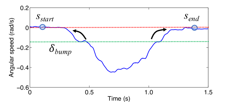
Figure 2: Left turn extraction from smoothed gyroscope readings.

S1. Recognizing steering maneuvers. Dri-Fi recognizes the occurrence of a steering maneuver when the yaw rate readings from the gyroscope form a “bump-shape”. When a car changes its direction by making a left turn, as shown in Fig. 2, the yaw rate reading from the gyroscope first decreases, reaches its minimum peak, and finally rises back to approximately 0 rad/s when the left turn is completed. For a right turn, everything would be the opposite to a left turn; increase, reach the maximum, and decrease. Depending on how the coordinates are aligned, a negative bump may reflect a right turn, not a left turn. However, in this paper, we consider the yaw rate to increase when rotated clock-wise. Based on this observation, Dri-Fi determines that a steering maneuver has occurred if the absolute yaw rate exceeds a certain threshold, $\delta_{bump}$, which is empirically set to 0.15  $rad/s$. Note that without the threshold ($\delta_{bump}$), even a small movement of the steering wheel would cause Dri-Fi to mis-detect a steering maneuver. Thus, Dri-Fi marks the start time/point of that steering maneuver as $s_{start}$ when the absolute yaw rate, $|Y|$, exceeded $\delta_{bump}$ for the first time. Also, Dri-Fi marks the end point, $s_{end}$, as when $|Y|$ first drops back below $\delta_{bump}$. Since the steering would in fact have started a bit before $s_{start}$ and ended a bit later than $s_{end}$, where $|Y|\approx 0$ as shown in Fig. 2, Dri-Fi moves points $s_{start}$ and $s_{end}$ backwards and forwards, respectively, until $|Y|\approx 0$. As a result, Dri-Fi interprets a steering maneuver to have made at a time within $s=[s_{start},s_{end}]$.

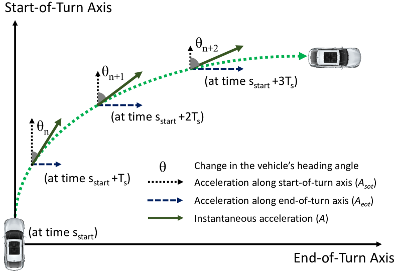
Figure 3: Changes in the vehicle’s accelerations and heading angle.

S2. Filtering left/right turns. The steering maneuver extracted in S1 may be comprised of not only left/right turns but also lane changes or U-turns, since those maneuvers yield similar bump-shaped yaw rate readings. In order to extract only left/right turns, as in [26], Dri-Fi derives the change in the vehicle’s heading angle, which is defined as the difference in the vehicle’s heading angle between the start and the end of a steering maneuver. Fig. 3 shows an example vehicle trajectory during a right turn where three IMU sensor readings were acquired at times $t=s_{start}+\{T_{s},2T_{s},3T_{s}\}$, i.e., sampled with frequency of $1/T_{s}$. As in step S1, let $t=s_{start}$ be the time when the vehicle was detected to have started the turn. Since the yaw rate readings from the gyroscope represent the vehicle’s angular velocity around the vertical (Z) axis, the change in the vehicle’s heading angle after time $nT_{s}$ has elapsed since $s_{start}$, $\theta[nT_{s}]$, can be approximated as

$$\theta[nT_{s}]\approx\theta[(n-1)T_{s}]+{Y_{n}T_{s}}=\sum\limits_{k=1}^{n}{Y_{k}T_{s}},$$ (1)

where $Y_{n}$ denotes the $n$-th yaw rate reading since $t=s_{start}$. Therefore, at the end of making a right turn, the eventual change in the vehicle’s heading angle, $\theta_{final}=\theta[s_{end}-s_{start}]$ would be approximately 90^∘ whereas at the end of a left turn it would be -90^∘. This change in the vehicle’s heading angle is a good indicator for determining whether the vehicle has made a left/right turn, since for lane changes, $\theta_{final}\approx 0^{\circ}$ whereas for U-turns, $\theta_{final}\approx 180^{\circ}$. Thus, Dri-Fi calculates the $\theta_{final}$ of a detected steering maneuver (made during $s_{start}\sim s_{end}$), and only retains it such that $70^{\circ}\leq|\theta_{final}|\leq 110^{\circ}$, i.e., approximately $\pm$90^∘. Note that since left/right turns usually take a short period of time ($<$3 seconds), drifting in the gyroscope during a turn [27] does not affect Dri-Fi’s performance.

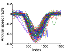
(a) Left turn.

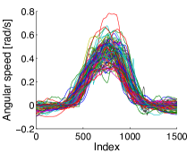
(b) Right turn.

Figure 4: Interpolated gyroscope readings.

As a result, whenever the driver makes a left/right turn, Dri-Fi can acquire a sensor data stream (i.e., gyroscope and accelerometer readings) which was output only during the turn, i.e., during $s=[s_{start},s_{end}]$. However, since different road geometries may result in different turning radii, the length of the readings may vary, which may affect the performance of Dri-Fi. Thus, in order to make Dri-Fi’s fingerprinting accuracy independent of path selection and only driver-dependent, we interpolate the sensor data stream into a fixed length. This also facilitates Dri-Fi to fingerprint the driver even when using two different devices that may have different sampling rates.

Fig. 4 shows the gyroscope readings of 12 different drivers’ left and right turns after interpolation; we will later elaborate in Section IV on how we collected them. Near-equivalent shapes of the gyroscope readings indicate that via interpolation, the analyses can be done from a consistent vantage point, despite turns being made on different road geometries. We will later show through evaluations that since the variance in left turn radii is usually much higher than that in right turns — as right turns usually start from only one lane — without such an interpolation, Dri-Fi’s fingerprinting accuracy drops more when using left-turn data than when using right-turn data.

III-D Maneuver-based Fingerprinting

Whenever driver $x$ (whose identity is not yet determined) makes a left/right turn, Dri-Fi acquires an IMU sensor data stream $\varphi^{x}_{turn}$. The main challenge in fingerprinting $x$ is determining which features to extract from the data stream.

Feature extraction. When drivers make either a left or right turn, one might notice that some drivers have their unique pattern in making the turn. Capturing such a pattern, Dri-Fi extracts the following three new features from the filtered IMU sensor data for driver fingerprinting:

• Acceleration along the end-of-turn axis ($A_{eot}$);

• Deviation of $F_{1}$ ($\Delta A_{eot}$); and

• Deviation of the raw yaw rate ($\Delta Y_{raw}$).

As depicted in Fig. 3, we define the start-of-turn (SOT) axis as the axis/direction in which the vehicle was detected to have started its turn (direction at time $s_{start}$). In reference to the SOT axis, we define the end-of-turn (EOT) axis as the one orthogonal to the SOT axis. That is, regardless of the change in the vehicle’s heading angle after the turn (e.g., 95^∘ for a right turn), by definition, the EOT axis is set perpendicular to the SOT axis.

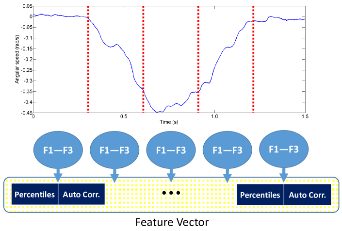
Figure 5: Dri-Fi’s construction of feature vector.

F₁. Acceleration along the EOT axis. The acceleration along the EOT axis is an interesting yet powerful feature in Dri-Fi since it represents both 1) how much the driver turns his/her steering wheel and 2) at that moment how hard the driver presses the brake/acceleration pedal during the left/right turn. In other words, it reflects one’s (unique) turning style. We will later show through extensive evaluations that the features we use for Dri-Fi do not depend on the vehicle type or route but only on the driver’s unique maneuvering style. Note that instantaneous acceleration, which we refer to as the acceleration along the vehicle’s heading axis, measured during a turn would only reflect the driver’s input/actions on the brake/acceleration pedal but not on the steering wheel. Similarly, the instantaneous yaw rate, i.e., the angular velocity of the vehicle, measured from the gyroscope sensor would only reflect the driver’s actions on the steering wheel.

For deriving the vehicle’s acceleration along the EOT axis when $nT_{s}$ seconds has elapsed since $s_{start}$, $A_{eot}[nT_{s}]$, Dri-Fi utilizes the vehicle’s instantaneous acceleration, $A[nT_{s}]$, at that moment (obtained from the accelerometer) and its change in the heading angle, $\theta[nT_{s}]$ (extracted from the gyroscope) as:

$$A_{eot}[nT_{s}]=A[nT_{s}]sin(\theta[nT_{s}]).$$ (2)

In addition to the acceleration along the EOT axis, the value along the SOT axis may also be used. However, since the information Dri-Fi would obtain from the accelerations along the SOT axis will be redundant when those along the EOT axis are already available, we do not consider them as features in Dri-Fi; this also reduces the feature space.

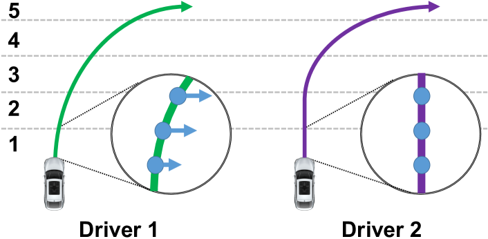
Figure 6: Different autocorrelations depending on the driver’s turning style.

As an alternative to $A_{eot}$, one can think of using centripetal/lateral acceleration, which would be perpendicular to the vehicle’s instantaneous acceleration ($A$). However, since the centripetal acceleration is affected by the turning radius, whereas the acceleration along the end-of-turn axis is not, we do not consider this for features in Dri-Fi.

F₂–F₃. Deviations of $A_{eot}$ and raw yaw rate. Dri-Fi derives not only $A_{eot}$ but also $\Delta A_{eot}$, i.e., difference between the subsequent acceleration values along the EOT axis. Since $\Delta A_{eot}$ reflects how aggressively the driver concurrently changes his steering and pedal actions during a turn, this feature captures the driver’s aggressiveness during the turn.

In addition to $\Delta A_{eot}$, Dri-Fi also determines the deviations in the raw yaw rate measurements, $\Delta Y_{raw}$. Note that in order to accurately extract left/right turns, Dri-Fi pre-processed the data with a low-pass filter. However, as the turns are already extracted, in order to not lose the accurate understanding/interpretation of how aggressively the driver turns his steering wheel, Dri-Fi also derives $\Delta Y_{raw}$; the driver’s aggressiveness shown from the low-pass filtered data would have been reflected in $F_{2}$. In addition to the driver’s aggressiveness of turning the steering wheel, this feature also captures how stable the driver maintains an angle during the turn(s) and thus helps Dri-Fi’s driver fingerprinting.

Feature Vector Construction. To construct the feature vector $\gamma_{turn}$ for classification and thus fingerprinting, Dri-Fi transforms $F_{1}$–$F_{3}$ as follows:

• Upon detection of a turn, as shown in Fig. 5, Dri-Fi divides the IMU sensor measurements (acquired during the turn) into 5 stages, each with an identical duration.

• For each stage, Dri-Fi determines $F_{1}$–$F_{3}$.

• For each of $F_{1}$–$F_{3}$, Dri-Fi determines its {10, 25, 50, 75, 90}-th percentiles and autocorrelations at 1–10 lags and aggregates them for constructing a feature vector.

Note that Dri-Fi generates an instance with such a feature vector per (detected) turn. With the percentiles, Dri-Fi understands the distributions of $F_{1}$–$F_{3}$ in each stage of turn.

Meanwhile, a more interesting and powerful feature for Dri-Fi in fingerprinting the driver is the autocorrelations of $F_{1}$–$F_{3}$ in each stage of turns. Fig. 6 shows an example of two different drivers making a right turn. When making the right turn, one can see that driver 1 started turning his steering wheel during stage 1 of the turn whereas driver 2 started it later during stage 3. As shown in Fig. 6, which also illustrates the accelerations along the EOT axis ($A_{eot}$) during stage 1, one can see that an early turn from driver 1 incurs non-zero values of $A_{eot}$ in stage 1 of the turn. On the other hand, since driver 2 drives further on a straight line along the SOT axis, his $A_{eot}$ values in stage 1 would approximately be 0. Similarly, values of $F_{2}$ and $F_{3}$ would also remain 0 for driver 2, but not for driver 1. As a result, the autocorrelations of $F_{1}$–$F_{3}$ for driver 1 would show significantly different values from those for driver 2, i.e., drivers’ different maneuvering styles lead to different $F_{1}$–$F_{3}$ autocorrelations during a turn.

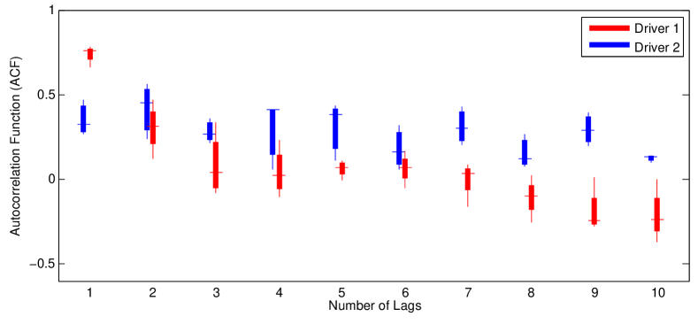
Figure 7: Correlogram of feature $F_{1}$ for two drivers.

Then, are these autocorrelation values of $F_{1}$–$F_{3}$ different enough between drivers to be considered as a driver’s fingerprint? Also, for a given driver, are those values consistent across multiple left/right turns? Fig. 7 shows the boxplots of $F_{1}$ autocorrelations for two drivers — who participated in our evaluations — during their first stage of left turns. We will later elaborate on the evaluation settings in Section IV. One can see that since the tendencies of drivers moving straight or turning the steering wheel early/late at the early stages of turns were different, the autocorrelations (at different lags) between the two drivers were obviously distinguishable. Moreover, one can see that although the driver was making those left turns at different times and places, the variances in some autocorrelation lags were quite low, i.e., stable. Not only the first stage but also stages 2$\sim$5 showed a similar distinctiveness and stability. This shows that the autocorrelations of $F_{1}$–$F_{3}$ are not only distinct among drivers but also quite stable for a given driver, i.e., drivers’ turning styles are relatively constant and distinct, so as to function as the core for Dri-Fi in fingerprinting the drivers.

Driver fingerprinting after a single turn. Using the constructed feature vector $\gamma^{x}_{turn}$ as an input and driver_profile_table as the training dataset for machine classifiers (e.g., Random Forest, SVM, Naive Bayes), Dri-Fi can fingerprint the driver as soon as the driver has made either a left or right turn, which we refer to as a “maneuver-based approach”. As shown in Fig. 1, driver_profile_table stores the drivers’ identities (e.g., Alice, Bob) and their corresponding driving data, $\Gamma_{turn}$. For now, we assume that the targeted driver/victim is within driver_profile_table, and this table is given to the adversary. Note that existing approaches for driver fingerprinting also assume this. Since this does not hold in some practical circumstances, we will discuss in Section III-F how the adversary may construct/obtain driver_profile_table from scratch via unsupervised machine learning.

III-E Trip-Based Fingerprinting

Albeit quite effective, when trying to fingerprint the driver within just one turn, some false positives/negatives may occur, possibly due to a sudden change in traffic signals, interruptions from pedestrians, etc. Hence, in order to reduce/remove such false positives/negatives, Dri-Fi can exploit the “accumulated” data obtained from multiple left/right turns within a trip that the driver is making, i.e., trip-based approach. Note that during a trip the driver remains the same.

One way the adversary might achieve this via Dri-Fi is by exploiting the Naive Bayes classifier, which is a simple probabilistic classifier based on the Bayes’ theorem. For a given vehicle driven by $N$ different drivers, assume that the adversary has a training set composed of several instances labeled as one of ${{D_{1}},\cdots,{D_{N}}}$. Then, within the trip in which the adversary attempts to fingerprint the driver, as the driver makes more turns, i.e., as more instances are collected, the adversary can estimate the maximum posterior probability (MAP) and thus predict the driver to be $D_{pred}$ as:

$$D_{pred}=\mathop{\arg\max}\limits_{k\in\left\{{{\rm{1,}}\cdots,N}\right\}}p\left({{D_{k}}}\right)\prod\limits_{i=1}^{n}{p\left({{T_{i}}|{D_{k}}}\right)},$$ (3)

where $n$ is the number of vehicle turns made up to the point of examination during the trip. Here, $p(T_{i}|D_{k})$ represents the likelihood that the (measured) $i$-th turn, $T_{i}$, would have occurred, given driver $D_{k}$ is driving the vehicle. Even though the adversary assumes that the prior probability, $p(D_{k})$ is equivalent across the (potential) drivers, i.e., each driver has an equal probability of driving that vehicle, we will later show through evaluations that the adversary can fingerprint the driver with higher accuracy than just using one turn, although, in most cases, one turn was sufficient in correctly fingerprinting the driver.

III-F Training Set Formulation

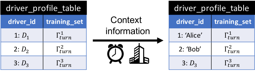
Figure 8: Formulating the training set (driver_profile_table) from scratch.

We now present how to construct driver_profile_table from scratch, thus enhancing Dri-Fi’s practicability. In constructing a valid training set, there exist two main challenges: 1) determine whether the new collected data comes from a driver the adversary had already learned about and 2) for the labeled data, exactly know who that driver would be. For the latter, without knowing this, the adversary would only be able to label the data as some variable $D_{i}$ rather than the driver’s actual identity (e.g., $D_{1}$=“Alice”); see Fig. 8 (left).

Determining a new driver. As illustrated in Fig. 1, once the adversary equipped with Dri-Fi collects $\gamma^{x}_{turn}$ from driver $x$, Dri-Fi determines whether driver $x$ would be one of the known/learned drivers or a new (unknown/unlearned) driver, i.e,. whether $x$ belongs to driver_profile_table. In the former, the adversary can expand the existing training set, whereas in the latter, he would have to construct a new training set for driver $x$. Such a process is essential, especially when the adversary starts, for the first time, to fingerprint the driver of a vehicle, i.e., starting from scratch.

Here, we briefly discuss how the adversary can indeed utilize unsupervised machine learning to correctly cluster/label $\gamma^{x}_{turn}$ to either an already-known or a new driver. What the adversary may do is label $\gamma^{x}_{turn}$ based on its log-likelihood obtained from a Gaussian mixture model (GMM). GMM is a combination of Gaussian component densities that are used for modeling the probability distribution of continuous measurements; see [28] for more details.

Suppose the adversary starts to fingerprint the driver(s). At first, since he has an empty training set, he first builds a GMM model, $M_{1}$, based on the training data $\Gamma^{1}_{turn}$ acquired during the vehicle’s first trip and labels it as (some) driver $D_{1}$. Then, during the next trip, when the adversary acquires $\gamma^{x}_{turn}$, he calculates the log-likelihood of $\gamma^{x}_{turn}$ given $M_{1}$. Accordingly, if the log-likelihood is high, meaning that $\gamma^{x}_{turn}$ is likely to be output from driver $D_{1}$, Dri-Fi appends $\gamma^{x}_{turn}$ to the associated training set $\Gamma^{1}_{turn}$. On the other hand, if the log-likelihood is low, $\gamma^{x}_{turn}$ is likely to have been generated by a new driver $D_{2}$ . Accordingly, Dri-Fi makes a new training set $\Gamma^{2}_{turn}$. In such a way, the adversary would able to construct the initial version of driver_profile_table (e.g., Fig. 8 (left)).

Accurately labeling the data. As shown in Fig. 8, the adversary can construct the training dataset more concretely if he knows exactly who $D_{1}$ is (e.g., $D_{1}$=“Alice”). This can be achieved not only via oversight but also based on other context information. For example, if the adversary knows that Alice always drives to work for an hour at 9:00 am on weekdays, the data being collected during 9:00$\sim$10:00 am is more likely to reflect Alice’s rather than other’s driving behavior. Other than time, useful context information such as location, phone usage patterns, DNS traffic pattern may also be utilized in verifying that the driver is indeed “Alice”. Note, however, that these are only valid when that context becomes available and is valid (e.g., on weekends, we are not sure that Alice is driving). Thus, we use context only for constructing the training dataset of Dri-Fi, but not for the actual fingerprinting.

In fact, such an approach would not only make the adversary build a concrete training set but also let him estimate the prior probability of a driver driving the vehicle — $p(D_{k})$ in Eq. (3) — and thus increase the fingerprinting accuracy.

In Section IV, we will show that the adversary can construct/obtain a well-formulated training set via this GMM approach. We also show through extensive evaluations that even when the training dataset obtains a few instances with incorrect labels (IV-F), i.e., a (slightly) defective training set due to the adversary’s mistake, he may still be able to identify the driver with high accuracy.

IV Evaluation

IV-A Evaluation Setup

To validate whether Dri-Fi accurately fingerprints the driver, we evaluated two imperative aspects of Dri-Fi: whether the derived features of Dri-Fi are 1) dependent only on the driver and 2) remain constant with various changing factors, e.g. car and/or route. To validate these, we started from a small-scale experiment where we varied/controlled different factors such as driver, car, route, which may (or may not) affect Dri-Fi’s performance. Once validated, to evaluate how Dri-Fi’s performance scales with high number of drivers, we conducted a large-scale experiment with more drivers driving in their own choice of car and routes. Overall, our driving data collection took 4 months and had more than 116 hours of driving data obtained from urban/suburban areas. The accumulated driving milage was 1,688 miles.

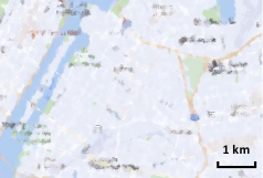
(a) Metropolitan area.

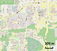
(b) Suburban area.

Figure 9: Different driving environments.

Data-collection methodology. The data-collection module of Dri-Fi was implemented as an Android app and was installed on various Android smartphones including Google Pixel, Nexus 5X, Samsung Galaxy S5, and Samsung Note 5. We recruited 12 (9 male and 3 female) drivers with an age span of 22–50. For collecting the data, we asked the drivers to 1) ensure the app is turned on before driving and 2) upload the data after finishing a trip. According to our survey after data collection, none of the participants indicated that our data collection app affected their normal driving pattern.

Since our system does not require any personal information from the users, the Institutional Review Boards (IRB) of our university classified this effort as non-regulated.

Tested vehicle and routes. The selection of vehicle and road were only controlled in our small-scale experiment. Specifically, to verify the factors which affect Dri-Fi’s performance, we asked two recruited drivers to drive a Honda Sedan and a Ford SUV. In the large-scale experiment, to validate that the derived features in Dri-Fi and thus its fingerprinting do not depend on the vehicle of choice, we allowed all participants to drive their own vehicle(s). As a result, we collected data from 10 cars of 7 different models: Honda Accord Sedan, Honda CRV SUV, Toyota Camry Sedan, Ford Explorer SUV, Hyundai Elantra Sedan, Jeep Compass SUV, and Toyota Corolla Sedan. Moreover, the routes were also freely chosen by the driver which included those in a suburban area with less traffic or a metropolitan area with heavy traffic; examples shown in Fig. 9.

IV-B Factor Analysis & Experimental Design

To verify that the fingerprinting accuracy of Dri-Fi only depends on the driver, not on the car or route, we first conducted a factor analysis via a small-scale experiment. As shown in Table I, we conducted 6 experiments, T1–T6, with same/different drivers, cars, and/or routes. For T7 (the large-scale experiment) where every factor was varied and uncontrolled, we will discuss later on how Dri-Fi performed.

Differentiated Factor(s)	Constant Factor(s)	Acc.
T1. Car	Driver, Route	Low
T2. Route	Driver, Car	Low
T3. Car, Route	Driver	Low
T4. Driver	Car, Route	High
T5. Driver, Car	Route	High
T6. Driver, Route	Car	High
T7. Driver, Car, Route	(None)	High

TABLE I: Summary of evaluations.

Test cases. For tests T1–T6, we varied/controlled the three factors as follows:

• Driver Factor: For test cases T4–T6 where the driver was differentiated, two different drivers were asked to drive a same/different car with specified instructions when needed, e.g., whether to drive on a pre-determined route.

• Car Factor: For test cases T1, T3, and T5 in which the car type was varied, we used two different cars: Honda Accord Sedan and a Ford Explorer SUV.

• Route Factor: For test cases T1, T4, and T5, where the route was fixed, we asked the drivers to drive around campus along the pre-determined route. For other test cases (T2, T3, and T6) where the route was differentiated, the route was solely determined by the drivers.

If Dri-Fi’s constructed features only depend on the driver factor, i.e., dependent on only the driver’s unique turning style, Dri-Fi’s performance in test cases T1–T3 would be low whereas in T4–T6, it should be high.

Classification. For each test case, we acquired data via Dri-Fi from two different trips, which differ in driver/car/route or a combination thereof (as shown in Table I). As the two trips (per test case) have distinct factors, we labeled the vehicle turns based on which trip they occurred. For example, in T1 where “car” was the only differentiated factor between the two trips, although the driver was identical, the vehicle turn data from each trip were labeled differently as 0 and 1, i.e., binary. Similarly in T6 where the “driver” and “route” were the differentiated factors, turns from each trip were again labeled 0 and 1. Based on the collected data from the two trips of cases T1–T6, we trained the classifiers using 90% of the turns and leave the remaining 10% as the test set. To obtain an accurate estimate of the model prediction performance, we used 10-fold cross validation. For each test case, as turns were from two different trips (with different drivers/cars/routes), we used binary classification. The classifiers we used for testing T1–T6 were Support Vector Machine (SVM) and a 100-tree Random Forest.

Performance. Fig. 10 plots accuracies of Dri-Fi in fingerprinting the driver based one single turn in T1–T6, when using SVM and Random Forest. Since the classification only needed to be binary, the classification accuracy of random guessing is 50%, which is shown as a horizontal dotted line.

One can see that for test cases T1–T3, although the vehicle and/or the route were different, Dri-Fi showed a very low classification accuracy: 66.6%, 64.2%, 61.1% using SVM, and 66.6%, 60.4%, 61.1% using Random Forest in cases T1–T3, respectively. Such a result can, in fact, be interpreted as having a similar accuracy as when it is guessed randomly. This also implies that regardless of the car or route used/taken, if the driver is identical, Dri-Fi gets confused.

When the ”driver” factor was changed as in test cases T4–T6, one can see from Fig. 10 that the classification accuracy of Dri-Fi was much higher: 96.3%, 91.7%, 94% using SVM, and 95%, 91.7%, 100% using Random Forest in cases T4–T6, respectively. Such a high classification accuracy was due to the fact that between the two trips of T4–T6, the drivers were different.

Based on these results, we can conclude that the features derived by Dri-Fi depends only on the driver and not on other factors such as car and/or route, thus functioning as the key for accurate driver fingerprinting. Moreover, Dri-Fi shows consistent performance across different machine classifiers.

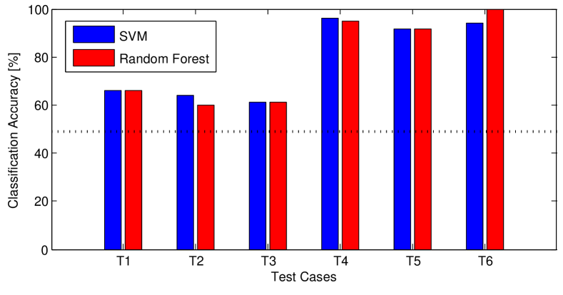
Figure 10: Classification accuracy for test cases T1–T6 using SVM and Random Forest.

IV-C Large-scale Experiment

To further evaluate Dri-Fi’s performance with more drivers, and to verify whether its derived features for a given driver remain consistent across different routes, we conducted a large-scale experiment: we used all the sensor data acquired from the 12 participants who drove 10 different cars. As most of these participants drove different cars on different routes, test case T7 represents such a setting.

In T7, since there were more than 2 drivers, when using SVM and Random Forest, we performed a multi-class classification. To achieve this, we examined it through one vs. one reduction rather than one vs. all since the former reflects more accurate results than the latter [29]. In the dataset, feature vectors of turns were labeled depending on who the driver was. Again, 10-fold cross validation was performed for an accurate performance measure.

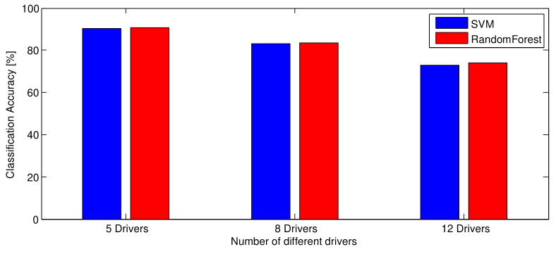
Figure 11: Dri-Fi’s accuracy in fingerprinting 5, 8, and 12 drivers within one vehicle turn using SVM and Random Forest.

Maneuver-based approach. We first evaluate how well Dri-Fi identifies 5, 8, and 12 drivers using a maneuver-based approach. Fig. 11 plots Dri-Fi’s accuracy in fingerprinting 5, 8, and 12 different drivers using SVM and Random Forest. One can see that within only one left/right turn, Dri-Fi can fingerprint the driver with 90.5%, 83.1%, and 72.8% accuracies across 5, 8, and 12 drivers, respectively, using SVM. When Random Forest is used, the fingerprinting accuracies were shown to be 90.8%, 83.5%, and 74.1% across the same driver sets. Although only mobile IMU sensors were used by Dri-Fi, thanks to its new features, Dri-Fi was able to identify the driver even though the number of drivers got larger; much better than random guessing. Such an achievement was made by observing only one left/right turn!

Trip-based approach. As discussed in Section III-E, instead of trying to fingerprint the driver based on one turn, the adversary may attempt to do it by accumulating sensor data of multiple turns collected within the trip, i.e., trip-based approach. To evaluate how well an adversary exploiting Dri-Fi may fingerprint the driver with such an approach, we evaluated Dri-Fi as follows. Per iteration, from our 12-driver driving dataset, we randomly selected one trip made by some driver; each driver made at least 2 trips. Then, we first randomly permuted the vehicle turns made within that trip and then considered those as our test set. Vehicle turns made in all other trips were considered as our training set. In predicting who the driver was in the (randomly) selected trip, i.e., the driver of the test set, we used the Naive Bayes classifier, which predicts the label based on the maximum a posteriori (as in Eq.(3)). The prior probability was set to be uniform. We performed such an evaluation 500 times.

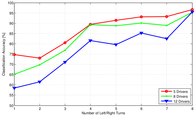
Figure 12: Classification accuracy of trip-based approach using Naive Bayes.

Fig. 12 plots Dri-Fi’s accuracy in identifying the driver correctly for the 500 iterations using a trip-based approach, when the number of candidate drivers were 5, 8, and 12. For evaluating the first two cases with 5 and 8 drivers, per iteration, they (as well as their trip/turn data) were randomly chosen from the total of 12 drivers. One can see that as more left/right turns were observed and analyzed by Dri-Fi, its classification accuracy continuously increased. After observing 8 left/right turns, Dri-Fi achieved fingerprinting accuracies of 96.6%, 95.4%, and 95.3% across 5, 8, and 12 drivers, respectively, which obviously is a great improvement over the “maneuver-based approach”, i.e., fingerprinting after one left/right turn. Since the way the drivers made their left/right turns was occasionally inconsistent, one more turn made by the driver did not necessarily increase Dri-Fi’s performance, i.e., performance did not monotonically increase. However, since the drivers made most of their turns according to their usual tendency/habit, ultimately the accuracy improved. Note that the accuracy of fingerprinting the driver via Naive Bayes after only one turn was a bit lower than when using other classifiers such as SVM or Random Forest due to its (naive) independence assumptions.

IV-D Efficacy of Interpolation

As discussed in Section III-C, to make Dri-Fi’s fingerprinting as independent as possible from the road geometry in which the turns are made, we interpolate the data to a fixed length. To evaluate the efficacy of such an interpolation, we evaluated Dri-Fi’s accuracy across 12 drivers when not executing such an interpolation.

	Left Turn		Right Turn
	SVM(%)	RF(%)	SVM(%)	RF(%)
w/ Interpolation	73.1	78.0	74.1	74.3
w/o Interpolation	65.2	72.0	71.5	72.2
Average difference	-6.95		-2.35

TABLE II: Efficacy of data interpolation.

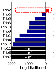
(a) Learned driver.

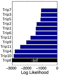
(b) New driver.

Figure 13: Using GMM for training set formulation.

Table II summarizes how Dri-Fi performed when fingerprinting the 12 drivers based on only left and right turns with/without interpolation. One can observe that when the data from different trips were not interpolated, the performance of Dri-Fi dropped. The reason for such a drop was that road geometries for different turns (even for the same driver) were not identical, i.e., the turning radii are different. So, through interpolation, Dri-Fi was able to remove the possible influence of the differences in turning radii, and thus achieve more accurate driver fingerprinting. Note that a driver’s turning radii can vary depending on where s/he is driving. Here, an interesting observation is that Dri-Fi’s accuracy dropped more when identifying the driver via left turn(s) than via right turn(s). This was because the turning radii for left turns normally have higher variations between them than for right turns; left turns can start from multiple lanes, whereas right turns (mostly) start from the rightmost lane.

IV-E Training Set Formulation

In Section III-F, we discussed how the adversary may use GMM to construct/obtain the training dataset for driver fingerprinting from scratch. To validate this, we considered the following case. Suppose that driver $D_{1}$ (w/o known identity) was the first to drive the vehicle since the adversary started to fingerprint its driver. Thus, the adversary constructs his initial training dataset, $\Gamma^{1}_{turn}$ with label $D_{1}$. In such a case, we examined what the GMM log-likelihood would be for the data collected from a new trip given $\Gamma^{1}_{turn}$.

Fig. 13(a) plots what the log-likelihood values were when data from 12 different trips, Trip1–Trip12 (each chosen from the 12 different drivers’ trips) were considered as the test set, thus being examined against the GMM of $\Gamma^{1}_{turn}$. We constructed $\Gamma^{1}_{turn}$ based on one of driver $D_{1}$’s trips, which was not included in the 12-trip test set. One can see that for only the data in Trip2, the log-likelihood was positive whereas for all others the values were negative or even negative infinite. This was because the driver of Trip2 was $D_{1}$. Such a result shows that by observing the GMM likelihood, the adversary can determine whether or not the newly collected data has been output by an existing driver in his training dataset. In this case, in Dri-Fi, the adversary would append the newly collected data from Trip2 to its initial dataset, $\Gamma^{1}_{turn}$.

This time, we randomly chose another trip from our 12-driver dataset and considered that as the adversary’s new initial training set, i.e., different $D_{1}$ and $\Gamma^{1}_{turn}$ (than the previous ones). We again considered the test set to be composed of 12 different trip data, but this time, made by drivers except for the chosen $D_{1}$. Fig. 13(b) plots the GMM log-likelihood values of data in the test set given the new $\Gamma^{1}_{turn}$. One can see that, since there were no trips within the test set taken by the same person as $D_{1}$, all showed negative/negative-infinite likelihoods. In such a case, Dri-Fi would determine that the newly collected data was output by a new driver, which he had not learned about, and thus construct a new training dataset for that driver.

IV-F Erroneous Training Dataset

When forming the training set via GMM, the standard for clustering new data was whether the GMM log-likelihood is positive or not. However, such a threshold setting may not always be reliable. Thus, to understand and evaluate how Dri-Fi’s performance will be affected when the adversary wrongly labels a turn while constructing the training dataset, e.g., a turn was made by driver 1 but the adversary labels it as by driver 2, from our dataset of 5 drivers, we arbitrarily picked and labeled some turns to be made by any of the 5 drivers. The number of arbitrarily picked turns with erroneous labels were varied via parameter $p_{err}$, which denotes the percentage of such erroneous labels. For this evaluation, we present the results obtained via SVM.

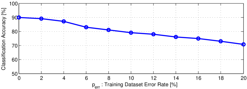
Figure 14: Classification accuracy with $p_{err}$ % erroneous training dataset.

Fig. 14 shows how Dri-Fi’s fingerprinting accuracy changed for $p_{err}$=0$\sim$20%. Even when the training dataset for Dri-Fi contains 20% of erroneous labels due to the adversary’s mistake, the adversary can still achieve 70.7% fingerprinting accuracy within only one turn. Despite the erroneous labels, such an accuracy can be increased further using a trip-based approach. Such a result implies that the adversary may not always have to be 100% accurate in constructing the training dataset in order to accurately fingerprint the driver with Dri-Fi, which is a serious threat.

IV-G Overhead of Dri-Fi

The additional overheads such as the CPU usage and energy consumption of Dri-Fi on the victim’s device may render the driver fingerprinting process noticeable by the victim.

To measure CPU usage, we recorded the CPU usage on both Google Pixel phone and Nexus 5X phone by using Android adb shell. To evaluate the extra overhead incurred by Dri-Fi’s data-collection module, which requires a bit higher sampling rate than usual, we compared the CPU usage of an application running with a normal IMU sampling rate (for detecting screen rotation) and with the sampling rate which Dri-Fi uses: 100Hz. As shown in Fig. 15(a), albeit the increased sampling rate of Dri-Fi, there were only small increases in the CPU usage; specifically, 2% increase on a Pixel phone and 3.4% increase on a Nexus 5X phone. Since such an increased CPU usage was also occasionally observable even when running with a normal sampling rate, the increased CPU usage may not necessarily indicate (or let the victim know) that Dri-Fi is running.

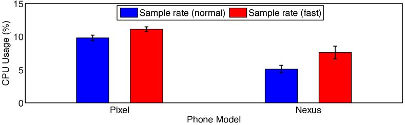
(a) CPU usage.

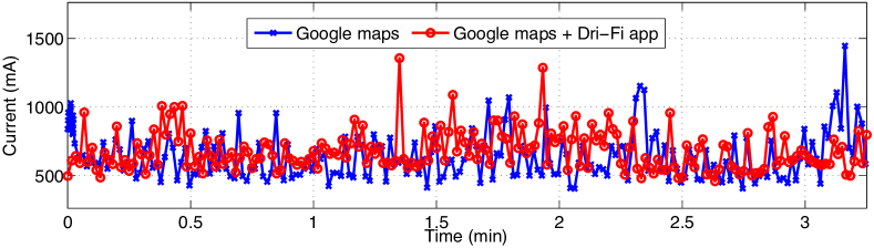
(b) Energy consumption.

Figure 15: Overhead of data collection app.

We also examined the additionally consumed energy of using Dri-Fi by measuring the current drawn in the smartphones. Fig. 15(b) shows the energy consumption on Pixel while Dri-Fi was running in the background and utility applications (e.g. Google maps) were running in the foreground. Our results indicate that compared to the case where Google maps drew 767.10mA of current for navigation, Dri-Fi drew only 49.60mA additional current. This 6.5% extra energy consumption would be too minimal for the victim to notice.

Such small increases in CPU usage and energy consumption imply that if the compromised app/software originally has high overhead (e.g., navigation and social apps), then this marginal increase of these overhead caused by Dri-Fi would be much less obvious. As a result, it will be even harder for the victim to notice such overheads.

V Related Work

V-A Device/User Tracking on Mobile Devices

While many researchers studied privacy invasion on mobile devices, their practicability in breaching the driver’s privacy is limited by a common requirement: the mobile device’s user/owner being tracked must also always be the driver.

A straightforward approach to identifying a mobile device is to track its unique identifier, such as IMEI, ICCID (SIM ID), etc., and/or cookies from its web browsers. However, this approach is not practical since reading unique identifiers requires the user’s permission and cookies can be easily deleted by the device user. To evade these, stealthier ways of tracking mobile devices have been explored. For example, Dey et al. [10] and Bojinov et al. [11] have shown adversaries to be able to track devices by utilizing the minor MEMS imperfection of the accelerometer. Resilient browser tracking approaches (e.g., evercookie [30]) have also shown a practical way of tracking devices that are connected to the Internet.

All of the above approaches are effective in identifying a device, but they share one common limitation in fingerprinting a driver: they cannot match the driving data with the user’s identity when the user is riding as a passenger. The motivating scenarios discussed in Section II-C are exemplars that the device-oriented approaches fail to fingerprint drivers. Note that even recent in-car phone localization methods — e.g., determining whether the phone is placed in the driver’s seat [31] — would also suffer from the same problem since the driver’s phone can be placed anywhere in the car, e.g., inside a purse sitting in the passenger’s seat.

Researchers have also been able to track the mobile user’s identity based on his/her behavioral pattern(s). For example, Bo et al. [13] constructed a “touch-based biometric” based on the user’s touch screen behavior and Herrmann et al. [14] used the user’s DNS traffic pattern to track him/her. Like device-oriented approaches, this type of tracking can also link the user’s current behavior with his/her identity. Note, however, that the user interacting with the device being tracked (while driving) may not necessarily be the driver.

V-B Driver Fingerprinting Based on CAN Data

Recently, various in-vehicle sensor data havebeen used to fingerprint drivers [3, 32, 4, 15, 16, 17].

Enev et al. [3] investigated whether an adversary can identify/fingerprint the driver via in-vehicle (specifically CAN) data. By exploiting 18 or more types of CAN sensor data (e.g., brake pedal position, throttle position, engine speed) collected through the OBD-II port for at least 15 minutes, the adversary was shown to be able to fingerprint the driver with high accuracy. Similarly, the feasibility of fingerprinting the driver based on CAN data was shown in [32].

Kwak et al. [17] also exploited CAN data for driver fingerprinting for an anti-theft purpose. In addition to the features proposed in [3], they exploited the mechanical features of automotive parts (e.g., transmission oil temperature), thus enhancing the accuracy of driver fingerprinting.

Hallac et al. [4] exploited 12 different types of CAN data for driver fingerprinting. Specifically, they proposed a classification algorithm by exploiting simple to complex features such as mean, standard deviation, and spectral components of the 12 different CAN sensor data. That way, they were able to identify the driver with high accuracy within one turn, but only when the number of different drivers were 2.

Van Ly et al. [15] also used in-car CAN data representing acceleration, brake, and turn signals to identify the driver. Other relevant work includes [16] which used not only CAN data but also additional new features including the car-following distance and the sound information when someone speaks inside the car for driver identification.

These related studies have demonstrated the feasibility of driver fingerprinting, but all of them are based on in-vehicle data. Both accessing and interpreting/decoding CAN data — i.e., knowing which CAN ID contains which sensor values and how they are encoded — are non-trivial problems.

In contrast, Dri-Fi takes a very different approach from existing driver fingerprinting schemes by identifying the driver based solely on mobile IMUs. Since these are zero-permission sensors and available in all commodity smartphones, some off-the-shelf devices, and even in OBD-II dongles, from an adversary’s point of view, the attack surface of fingerprinting drivers is much larger than that covered by existing schemes. For example, any malicious app installed on the victim’s smartphone can collect the IMU data. Moreover, Dri-Fi can achieve driver fingerprinting with high accuracy as soon as the driver makes a single turn. Even though Dri-Fi can sometimes be incorrect after the first turn, as the driver makes more turns and thus Dri-Fi collects more data, its accuracy of fingerprinting improves significantly.

VI Discussion

Number of drivers. We evaluated Dri-Fi with up to 12 drivers. The fact that an adversary can accurately fingerprint the driver among such a number of candidates (even with access to only IMUs) implies a serious potential privacy risk. In most real-world scenarios, the maximum number of drivers for a given vehicle may not even be that large. Privately owned vehicles — the most common scenario — will most probably be driven by only a few people, such as family members. Although the accuracy of Dri-Fi’s maneuver-based fingerprinting approach drops as the number of driver increases (Fig. 10), Dri-Fi can offset such a deterioration via a trip-based fingerprinting approach; as shown in Fig. 12, Dri-Fi can boost the accuracy with increasing number of turns.

Countermeasures. To prevent an adversary from fingerprinting the driver via an IMU, one may add artificial noise to the sensor readings. Addition of noise does not necessarily have to be done continuously, but only when the driver is anticipated to start his turn. For example, as in Fig. 2, when the absolute gyroscope readings exceed the threshold, $\delta_{bump}$, the device can be configured to add noise. Accordingly, an adversary exploiting Dri-Fi would be unable to extract accurate measurements from a vehicle turn and thus fail in driver fingerprinting. For smartphones, such an approach should be implemented in the OS-level, if there are no other apps using IMU sensors for “good purposes” while driving. Another countermeasure (in case of a smartphone) is to request permission for use of IMU sensors when installing the app, as discussed in [27].

Limitations. With the coordinate alignment discussed in Sec. III-B, Dri-Fi can analyze the data from a consistent viewpoint, i.e., according to the geo-frame coordinate, no matter what the posture of the device has. However, if the device always moves during driving (e.g., the driver’s smartwatch), it may introduce noise in the measurements, thus rendering Dri-Fi to be less accurate. Moreover, depending on the driver’s emotion, sense of urgency, and physical status, Dri-Fi’s accuracy may vary as well. In fact, the false-positives/negatives in Dri-Fi’s fingerprinting might occur for these reasons. So, in future we would like to conduct a detailed study of the effects of such factors on Dri-Fi’s accuracy.

VII Conclusion

In this paper, we presented Dri-Fi, a driving data analytic engine that an adversary can exploit to fingerprint the driver within only one vehicle turn, and most importantly using only zero-permission mobile IMUs. Dri-Fi achieves this by capturing new representative features of a driver’s unique way of making turns. Via extensive evaluations, Dri-Fi’s extracted features are shown to represent the driver’s unique turning style and thus function as the key in fingerprinting the driver. Such a feature of Dri-Fi implies a significant expansion of the attack vector; an adversary can identify the driver with access to not only in-car data but also to IMU-equipped devices. More importantly, it implies a practical, serious, and a yet uncovered privacy threat. Accordingly, we suggest both academia and industry to be wary of such a threat and thus make concerted efforts to develop countermeasures.

References

- [1] “Driver Privacy Act,” https://www.congress.gov/bill/114th-congress/house-bill/22/text#toc-H7E76328B2CD946219201C9FF6470C491, 2015.
- [2] “NHTSA, U.S. Dep’t of Transp., Privacy Impact Assessment,” https://cms.dot.gov/sites/dot.gov/files/docs/Privacy%20-%20NHTSA%20-%20V2V%20NPRM%20-%20PIA%20-%20Approved%20-%20122016.pdf, 2017.
- [3] M. Enev, A. Takakuwa, K. Koscher, and T. Kohno, “Automobile driver fingerprinting,” in Proceedings on Privacy Enhancing Technologies, 2016, pp. 34–50.
- [4] D. Hallac, A. Sharang, R. Stahlmann, A. Lamprecht, M. Huber, M. Roehder, R. Sosič, and J. Leskovec, “Driver identification using automobile sensor data from a single turn,” in 2016 IEEE 19th International Conference on Intelligent Transportation Systems (ITSC), Nov 2016, pp. 953–958.
- [5] “German car industry plans to close OBD interface [Online] http://www.eenewsautomotive.com/news/german-car-industry-plans-close-obd-interface,” 2017.
- [6] K.-T. Cho and K. G. Shin, “Fingerprinting Electronic Control Units for Vehicle Intrusion Detection,” in Proc. of the 25th USENIX Security Symposium, Aug. 2016.
- [7] ——, “Error Handling of In-vehicle Networks Makes Them Vulnerable,” in Proc. of the 23rd ACM Conference on Computer and Communications Security (CCS), Oct. 2016.
- [8] “TrueMotion,” https://gotruemotion.com/, 2017.
- [9] “Usage based insurance,” https://en.wikipedia.org/wiki/Usage-based_insurance, 2017.
- [10] S. Dey, N. Roy, W. Xu, R. R. Choudhury, and S. Nelakuditi, “Accelprint: Imperfections of accelerometers make smartphones trackable.” in NDSS, 2014.
- [11] H. Bojinov, Y. Michalevsky, G. Nakibly, and D. Boneh, “Mobile device identification via sensor fingerprinting,” arXiv:1408.1416, 2014.
- [12] J. R. Mayer and J. C. Mitchell, “Third-party web tracking: Policy and technology,” in 2012 IEEE Symposium on Security and Privacy, May 2012.
- [13] C. Bo, L. Zhang, X.-Y. Li, Q. Huang, and Y. Wang, “Silentsense: Silent user identification via touch and movement behavioral biometrics,” in Proceedings of the 19th Annual International Conference on Mobile Computing; Networking, ser. MobiCom ’13. ACM, 2013, pp. 187–190.
- [14] D. Herrmann, C. Banse, and H. Federrath, “Behavior-based tracking: Exploiting characteristic patterns in dns traffic,” 2013.
- [15] M. V. Ly, S. Martin, and M. M. Trivedi, “Driver classification and driving style recognition using inertial sensors,” in 2013 IEEE Intelligent Vehicles Symposium (IV), June 2013, pp. 1040–1045.
- [16] C. Miyajima, Y. Nishiwaki, K. Ozawa, T. Wakita, K. Itou, K. Takeda, and F. Itakura, “Driver modeling based on driving behavior and its evaluation in driver identification,” Proceedings of the IEEE, vol. 95, no. 2, pp. 427–437, Feb 2007.
- [17] B. I. Kwak, J. Woo, and H. K. Kim, “Know your master: Driver profiling-based anti-theft method,” in Privacy, Security and Trust (PST), June 2016, pp. 1040–1045.
- [18] I. Foster, A. Prudhomme, K. Koscher, and S. Savage, “Fast and vulnerable: A story of telematic failures,” in Proceedings of the 9th USENIX Conference on Offensive Technologies, ser. WOOT’15, 2015.
- [19] “Volvo: use smartphone to unlock cars,” https://www.theverge.com/2016/2/19/11059592/volvo-phone-car-key-app-ride-sharing, 2016.
- [20] “Tesla Model 3 has no key: so don’t forget your phone,” https://www.cnet.com/roadshow/news/tesla-model-3-has-no-key-so-dont-forget-your-phone/#, 2017.
- [21] “Name driver exclusion,” http://www.insure.com/car-insurance/exclusions.html, 2017.
- [22] “Progressive’s note on excluded drivers,” https://www.progressive.com/glossary/, 2016.
- [23] “DMV’s alert about named driver exclusion,” http://www.dmv.org/insurance/auto-insurance-exclusion.php, 2016.
- [24] “The OpenXC Platform,” http://openxcplatform.com/, 2012.
- [25] “Intel OBD-II Dongle,” https://www.intel.com/content/dam/www/public/us/en/documents/product-briefs/vehicle-telematics-solution-product-brief.pdf, 2017.
- [26] D. Chen, K.-T. Cho, S. Han, Z. Jin, and K. G. Shin, “Invisible sensing of vehicle steering with smartphones,” in Proceedings of the 13th Annual International Conference on Mobile Systems, Applications, and Services, ser. MobiSys ’15. ACM, 2015, pp. 1–13.
- [27] S. Narain, T. Vo-Huu, K. Block, and G. Noubir, “Inferring User Routes and Locations Using Zero-permission Mobile Sensors,” in IEEE Symposium on Security and Privacy, May. 2016.
- [28] D. Reynolds and R. Rose, “Robust Text-Independent Speaker Identification Using Gaussian Mixture Speaker Models,” in IEEE Transactions on Speech and Audio Processing, Jan. 1995.
- [29] S. Park and J. Furnkranz, “Efficient pairwise classification,” in Machine Learning: ECML 2007, pages 658-665. Springer,, 2007.
- [30] “Evercookie,” https://github.com/samyk/evercookie, 2010.
- [31] H. Chu, V. Raman, J. Shen, A. Kansal, V. Bahl, and R. R. Choudhury, “I am a smartphone and i know my user is driving,” in 2014 Sixth International Conference on Communication Systems and Networks (COMSNETS), 2014.
- [32] B. Wang, S. Panigrahi, M. Narsude, and A. Mohanty, “Driver identification using vehicle telematics data,” in SAE Technical Paper. AE International, 2017.