Higher-order Fermi-liquid corrections for an Anderson impurity away from half-filling III: non-equilibrium transport

Abstract

We extend the microscopic Fermi-liquid theory for the Anderson impurity [Phys. Rev. B 64, 153305 (2001)] to explore non-equilibrium transport at finite magnetic fields. Using the Ward identities in the Keldysh formalism with the analytic and anti-symmetric properties of the vertex function, the spin-dependent Fermi-liquid corrections of order $T^{2}$ and $(eV)^{2}$ are determined at low temperatures $T$ and low bias voltages $eV$. Away from half-filling, these corrections can be expressed in terms of the linear and non-linear static susceptibilities which represent the two-body and three-body fluctuations, respectively. We calculate the non-linear susceptibilities using the numerical renormalization group, to explore the differential conductance $dI/dV$ through a quantum dot. We find that the two-body fluctuations dominate the corrections in the Kondo regime at zero magnetic field. The contribution of the three-body fluctuations become significant far away from half-filling, especially in the valence-fluctuation regime and empty-orbital regimes. In finite magnetic fields, the three-body contributions become comparable to the two-body contributions, and play an essential role in the splitting of the zero-bias conductance peak occurring at a magnetic field of the order of the Kondo energy scale. We also apply our microscopic formulation to the magneto-resistance and thermal conductivity of dilute magnetic alloys away from half-filling.

I Introduction

It has already been more than forty years since Nozières’ phenomenological Fermi-liquid theory for the Kondo systemNozières (1974) and the corresponding microscopic description of Yamada-Yosida Yamada (1975a, b); Shiba (1975); Yoshimori (1976) successfully explained the universal low-energy behavior, which had been clarified by Wilson’s numerical normalization group (NRG).Wilson (1975); Krishna-murthy et al. (1980a, b) Recently, there has been a significant breakthrough, which extends Nozières’ phenomenological description and reveals higher-order Fermi-liquid corrections in the particle-hole asymmetric case.Mora et al. (2015); Filippone et al. (2017) Specifically, Filippone, Moca, von Delft and Mora (FMvDM) have presented the low-energy asymptotic form of the Green’s function $G_{\sigma}(\omega)$ up to terms of order $\omega^{2}$, $T^{2}$, and $(eV)^{2}$, at finite temperatures $T$, bias voltages $V$, and magnetic fields.Filippone et al. (2017) It shed light on a long standing problem in the Kondo physics away from half-filling, which has been studied for dilute magnetic alloysNozières (1974); Yamada (1975a, b); Shiba (1975); Yoshimori (1976) and quantum dots.Hershfield et al. (1992); Oguri (2001); Aligia (2012); Muñoz et al. (2013)

In the previous two papers,Oguri and Hewson ; Oguri and Hewson (2018) we provided a microscopic description for the higher-order Fermi-liquid corrections away from half-filling, extending the approach of Yamada-Yosida using Ward identities. We have shown that the next-leading Fermi-liquid corrections, which cannot be neglected away from half-filling, are deduced from one of the key features of the vertex function for parallel spins: the $\omega$-linear term of $\Gamma_{\sigma\sigma;\sigma\sigma}(\omega,0;0,\omega)$ becomes pure imaginary with no real part at $T=0$ and $eV=0$. The additional Fermi-liquid parameters can be expressed in terms of the static three-body correlation functions of the impurity occupations, i.e., $n_{d\sigma}$’s. The first paper is a letter, in which have described an overview of the results that follow from this property.Oguri and Hewson It has been proved in the second paper, hereafter referred to as paper II, that the fermionic anti-symmetry property causes the absence of an $\omega$-linear term in the real part of $\Gamma_{\sigma\sigma;\sigma\sigma}(\omega,0;0,\omega)$.Oguri and Hewson (2018) In addition, we have also calculated the $\omega^{2}$ and $T^{2}$ real part of the self-energy at equilibrium using the Matsubara imaginary-time Green’s function.Filippone et al. (2017)

In the present paper, we continue the precise discussion started in paper II. We microscopically derive the low-energy asymptotic form of the Keldysh Green’s function, extending the non-equilibrium Ward identities for finite magnetic fields.Oguri (2001) We also calculate the Fermi-liquid corrections to transport through a quantum dot Glazman and Raikh (1988); Ng and Lee (1988); Hershfield et al. (1992); Wingreen and Meir (1994); Meir and Wingreen (1992) and also thermoelectric transportCosti et al. (1994); Oguri and Maekawa (1990) in dilute magnetic alloys away from half-filling. In addition, we apply the microscopic description to the multi-orbital case with $N$ impurity components, and present the precise form of the expansion coefficients for the self-energy. The result of the order $\omega^{2}$ real part of the self-energy, which has been deduced from the Ward identity, completely agrees with the FMvDM’s formula.Filippone et al. (2017)

In order to see how the higher-order Fermi-liquid parameters evolve as the system deviates from the particle-hole symmetric point, we also explore some typical cases using the NRG. The corrections away from the symmetric case are determined not only by the two-body fluctuations which enter through the linear susceptibilities $\chi_{\sigma\sigma^{\prime}}$ but the three-body fluctuations described by the static nonlinear susceptibilities $\chi_{\sigma_{1}\sigma_{2}\sigma_{3}}^{[3]}$. Specifically, we see that each of these two types of the fluctuations contributes to the $T^{2}$ and $(eV)^{2}$ Fermi-liquid corrections for the conductance through a quantum dot away from half-filling, and also at finite magnetic fields. The result shows that at zero field the contributions of the two-body fluctuations dominate in the Kondo regime, whereas the three-body fluctuations are significant in valence fluctuation and empty-orbital regimes. In contrast, in the case where a magnetic field is applied to the Kondo regime, both the two-body and three-body fluctuations give comparable contributions to the $T^{2}$ and $(eV)^{2}$ corrections. We also discuss how these two types of fluctuations contribute to the $T^{2}$ corrections of the electric resistance and thermal conductivity of the dilute magnetic alloys.

The paper is organized as follows. In Sec. II, static non-linear susceptibilities and the Ward identities which have been described in paper II are summarized. The non-equilibrium Ward identities for finite magnetic fields are derived in Sec. III. The results for the asymptotic form of the retarded self-energy is described in Sec. IV. Then, in Sec. V, differential conductance of quantum dot is discussed at symmetric tunneling couplings. In Sec. VI, we apply the microscopic Fermi-liquid description to thermoelectric transport of dilute magnetic alloy away from half-filling. A summary is given in Sec. VII.

II Formulation and summary of equilibrium properties

We study the transport properties in the Fermi-liquid regime away from half-filling in this paper. We consider the single Anderson impurity coupled to two noninteracting leads: $\mathcal{H}=\mathcal{H}_{d}+\mathcal{H}_{c}+\mathcal{H}_{\mathrm{T}}$,

$$\mathcal{H}_{d}= \ \sum_{\sigma}\epsilon_{d\sigma}\,n_{d\sigma}+U\,n_{d\uparrow}\,n_{d\downarrow},$$ (1)

$$\mathcal{H}_{c}= \ \sum_{\lambda=L,R}\sum_{\sigma}\int_{-D}^{D}\!\!d\epsilon\,\epsilon\,c^{\dagger}_{\epsilon\lambda\sigma}c_{\epsilon\lambda\sigma},$$ (2)

$$\mathcal{H}_{\mathrm{T}}= \ \sum_{\lambda=L,R}\sum_{\sigma}v_{\lambda}\left(\psi_{\lambda,\sigma}^{\dagger}d_{\sigma}+d_{\sigma}^{{\dagger}}\psi_{\lambda,\sigma}\right).$$ (3)

Here, $d^{{\dagger}}_{\sigma}$ creates an impurity electron with spin $\sigma$ in the impurity level of energy $\epsilon_{d\sigma}$, and $n_{d\sigma}=d^{{\dagger}}_{\sigma}d_{\sigma}$. $U$ is the Coulomb interaction between electrons occupying the impurity level. Conduction electrons in the two leads at $\lambda=L$ and $R$ obey the anti-commutation relation $\{c^{\phantom{\dagger}}_{\epsilon\lambda\sigma},c^{\dagger}_{\epsilon^{\prime}\lambda^{\prime}\sigma^{\prime}}\}=\delta_{\lambda\lambda^{\prime}}\,\delta_{\sigma\sigma^{\prime}}\delta(\epsilon-\epsilon^{\prime})$. The linear combination of the conduction electrons, $\psi_{\lambda\sigma}\equiv\int_{-D}^{D}d\epsilon\sqrt{\rho_{c}}\,c^{\phantom{\dagger}}_{\epsilon\lambda\sigma}$ with $\rho_{c}=1/(2D)$, couples to the impurity level. The bare width is given by $\Delta\equiv\Gamma_{L}+\Gamma_{R}$ with $\Gamma_{\lambda}=\pi\rho_{c}v_{\lambda}^{2}$. We consider the parameter region, where the half band-width $D$ is much greater than the other energy scales, $D\gg\max(U,\Delta,|\epsilon_{d\sigma}|,|\omega|,T,eV)$. For finite magnetic fields $h$, the impurity energy takes the form $\epsilon_{d\sigma}=\epsilon_{d}-\sigma h$, where $\sigma=+1$ (-1) for $\uparrow$ ($\downarrow$) spin. The relation between the differentiations is

$$\frac{\partial}{\partial\epsilon_{d}}=\frac{\partial}{\partial\epsilon_{d\uparrow}}+\frac{\partial}{\partial\epsilon_{d\downarrow}},\qquad\frac{\partial}{\partial h}=-\frac{\partial}{\partial\epsilon_{d\uparrow}}+\frac{\partial}{\partial\epsilon_{d\downarrow}},$$ (4)

and $\frac{\partial}{\partial\epsilon_{d\sigma}}=\frac{1}{2}\left(\frac{\partial}{\partial\epsilon_{d}}-\sigma\,\frac{\partial}{\partial h}\right)$.

II.1 Local Fermi-liquid parameters in equilibrium

II.1.1 Free energy $\Omega$ and Green’s function at $T=0$

The low-bias behavior of the self-energy can be deduced from the equilibrium quantities. Specifically, at $T=0$ and $eV=0$, the usual zero-temperature formalism is applicable to the causal Green’s function defined with respect to the equilibrium ground state,

$$G_{\mathrm{eq},\sigma}^{--}(\omega)\ = \ -i\,\int_{-\infty}^{\infty}dt\,e^{i\omega t}\langle\,\mbox{T}\,d^{\phantom{\dagger}}_{\sigma}(t)\,d^{\dagger}_{\sigma}(0)\,\rangle$$

$$= \ \frac{1}{\omega-\epsilon_{d\sigma}+i\Delta\,\mathrm{sgn}\,\omega-\Sigma_{\mathrm{eq},\sigma}^{--}(\omega)}\;.$$ (5)

The corresponding $T=0$ retarded Green’s function is given by $G_{\mathrm{eq},\sigma}^{r}(\omega)=\ \theta(\omega)G_{\mathrm{eq},\sigma}^{--}(\omega)+\theta(-\omega)\left\{G_{\mathrm{eq},\sigma}^{--}(\omega)\right\}^{*}$, where $\theta(\omega)$ is the Heaviside step function. The density of states for impurity electrons is defined by

$$\rho_{d\sigma}(\omega)\,\equiv\,-\,\frac{1}{\pi}\,\mathrm{Im}\,G_{\mathrm{eq},\sigma}^{r}(\omega)\;.$$ (6)

We will write the density of states at the Fermi energy $\omega=0$ in the following way, suppressing the frequency argument $\rho_{d\sigma}\equiv\rho_{d\sigma}(0)={\sin^{2}\delta_{\sigma}}/{\pi\Delta}$, where

$$\delta_{\sigma}\,=\,\cot^{-1}\left[\frac{\epsilon_{d\sigma}+\Sigma_{\mathrm{eq},\sigma}^{r}(0)}{\Delta}\right].$$ (7)

The phase shift $\delta_{\sigma}$ is a primary parameter which characterizes the Fermi-liquid ground state. The Friedel sum rule relates the phase shift to the occupation number which also corresponds to the first derivative of the free energy $\Omega\equiv-T\log\left[\mathrm{Tr}\,e^{-\mathcal{H}/T}\right]$,

$$\langle n_{d\sigma}\rangle\,=\,\frac{\partial\Omega}{\partial\epsilon_{d\sigma}}\,\xrightarrow{\,T\to 0\,}\,\frac{\delta_{\sigma}}{\pi}\;.$$ (8)

II.1.2 Second derivative of $\Omega$

The leading Fermi-liquid corrections can be described by the static susceptibilities following Yamada-Yosida:Yamada (1975a)

$$\chi_{\sigma\sigma^{\prime}}\equiv-\frac{\partial^{2}\Omega}{\partial\epsilon_{d\sigma^{\prime}}\partial\epsilon_{d\sigma}}=-\,\frac{\partial\langle n_{d\sigma}\rangle}{\partial\epsilon_{d\sigma^{\prime}}}\,\xrightarrow{\,T\to 0\,}\,\rho_{d\sigma}\,\widetilde{\chi}_{\sigma\sigma^{\prime}}.\!\!$$ (9)

Note that $\chi_{\uparrow\downarrow}=\chi_{\downarrow\uparrow}$. The renormalization factors are defined by

$$\!\!\!\widetilde{\chi}_{\sigma\sigma^{\prime}}\!\equiv\delta_{\sigma\sigma^{\prime}}\!+\!\frac{\partial\Sigma_{\mathrm{eq},\sigma}^{r}(0)}{\partial\epsilon_{d\sigma^{\prime}}},\ \ \,\frac{1}{z_{\sigma}}\!\equiv 1\!-\!\left.\frac{\partial\Sigma_{\mathrm{eq},\sigma}^{r}(\omega)}{\partial\omega}\right|_{\omega=0}\!\!.\!\!\!$$ (10)

The susceptibility can be written as a static 2-body correlation function

$$\chi_{\sigma\sigma^{\prime}}= \ \int_{0}^{1/T}\!\!d\tau\,\left\langle\delta n_{d\sigma}(\tau)\,\delta n_{d\sigma^{\prime}}\right\rangle,$$ (11)

where $\delta n_{d\sigma}\equiv n_{d\sigma}-\langle n_{d\sigma}\rangle$. The usual spin and charge susceptibilities are given by

$$\!\!\!\chi_{c}\,\equiv \ -\frac{\partial^{2}\Omega}{\partial\epsilon_{d}^{2}}\,=\,\chi_{\uparrow\uparrow}+\chi_{\downarrow\downarrow}+\chi_{\uparrow\downarrow}+\chi_{\downarrow\uparrow}\;,$$ (12a)

$$\!\!\!\chi_{s}\,\equiv \ -\frac{1}{4}\frac{\partial^{2}\Omega}{\partial h^{2}}\,=\,\frac{1}{4}\left(\,\chi_{\uparrow\uparrow}+\chi_{\downarrow\downarrow}-\chi_{\uparrow\downarrow}-\chi_{\downarrow\uparrow}\,\right).$$ (12b)

The free energy $\Omega$ is an even function of the field $h$. Therefore, $\chi_{c}$ and $\chi_{s}$ are also even functions of $h$. Furthermore, $\chi_{\uparrow\downarrow}$ is an even function of $h$,

$$\chi_{\uparrow\downarrow}=\chi_{\downarrow\uparrow}=-\frac{\partial^{2}\Omega}{\partial\epsilon_{d\uparrow}\partial\epsilon_{d\downarrow}}=-\frac{1}{4}\left(\frac{\partial^{2}\Omega}{\partial\epsilon_{d}^{2}}-\frac{\partial^{2}\Omega}{\partial h^{2}}\right).$$ (13)

Similarly, $\chi_{\uparrow\uparrow}+\chi_{\downarrow\downarrow}$ is an even function of $h$, and $\chi_{\uparrow\uparrow}-\chi_{\downarrow\downarrow}$ is an odd function of $h$:

$$\chi_{\uparrow\uparrow}+\chi_{\downarrow\downarrow}\,= \ -\frac{1}{2}\left(\frac{\partial^{2}\Omega}{\partial\epsilon_{d}^{2}}+\frac{\partial^{2}\Omega}{\partial h^{2}}\right)\;,$$ (14a)

$$\chi_{\uparrow\uparrow}-\chi_{\downarrow\downarrow}\,= \ \frac{\partial}{\partial\epsilon_{d}}\left(\frac{\partial\Omega}{\partial h}\right)\;.$$ (14b)

Therefore, $\chi_{\uparrow\uparrow}=\chi_{\downarrow\downarrow}$ at zero field $h=0$.

II.1.3 Third derivative of $\Omega$

The next leading Fermi-liquid corrections are determined by the static nonlinear susceptibilities, as we will describe later,

$$\chi_{\sigma_{1}\sigma_{2}\sigma_{3}}^{[3]}\equiv\ -\,\frac{\partial^{3}\Omega}{\partial\epsilon_{d\sigma_{1}}\partial\epsilon_{d\sigma_{2}}\partial\epsilon_{d\sigma_{3}}}\,=\,\frac{\partial\chi_{\sigma_{2}\sigma_{3}}}{\partial\epsilon_{d\sigma_{1}}}.$$ (15)

It also corresponds to the thee-body correlations of the impurity occupation

$$\chi_{\sigma_{1}\sigma_{2}\sigma_{3}}^{[3]}\!=-\!\int_{0}^{\frac{1}{T}}\!\!\!d\tau_{3}\!\!\int_{0}^{\frac{1}{T}}\!\!\!d\tau_{2}\,\langle T_{\tau}\delta n_{d\sigma_{3}}(\tau_{3})\,\delta n_{d\sigma_{2}}(\tau_{2})\,\delta n_{d\sigma_{1}}\rangle.$$ (16)

Similarly, the $n$-th derivative of $\Omega$ for $n=4,5,6\cdots$ corresponds to the $n$-body correlation function $\chi_{\sigma_{1}\sigma_{2}\sigma_{3}\cdots}^{[n]}$. The Fermi-liquid corrections can be classified according to $n$, and the derivative of the Ward identity reveals a hierarchy of Fermi-liquid relations, as described in the next subsection.

The $n$-body correlation function have permutation symmetry for the spin indexes $\chi_{\sigma_{1}\sigma_{2}\sigma_{3}\cdots}^{[n]}=\chi_{\sigma_{2}\sigma_{1}\sigma_{3}\cdots}^{[n]}=\chi_{\sigma_{3}\sigma_{2}\sigma_{1}\cdots}^{[n]}=\cdots$, and thus it has $n+1$ independent components at finite magnetic fields. There are four independent components for the $n=3$ case:

$$\frac{\partial\chi_{\uparrow\downarrow}}{\partial\epsilon_{d\sigma}}\,= \ \frac{1}{2}\left(\frac{\partial\chi_{\uparrow\downarrow}}{\partial\epsilon_{d}}-\sigma\frac{\partial\chi_{\uparrow\downarrow}}{\partial h}\right)\,\xrightarrow{\,h\to 0\,}\,\frac{1}{2}\frac{\partial\chi_{\uparrow\downarrow}}{\partial\epsilon_{d}}\;,$$ (17)

$$\frac{\partial\chi_{\sigma\sigma}}{\partial\epsilon_{d\sigma}}\ = \ \frac{\partial\chi_{\sigma\sigma}}{\partial\epsilon_{d}}-\frac{\partial\chi_{\uparrow\downarrow}}{\partial\epsilon_{d\sigma}}\xrightarrow{\,h\to 0\,}\,\frac{\partial\chi_{\uparrow\uparrow}}{\partial\epsilon_{d}}-\frac{1}{2}\frac{\partial\chi_{\uparrow\downarrow}}{\partial\epsilon_{d}}.$$ (18)

for $\sigma=\uparrow,\downarrow$. At zero field $h=0$, only two components are independent because $\chi_{\uparrow\uparrow\uparrow}^{[3]}=\chi_{\downarrow\downarrow\downarrow}^{[3]}$ and $\chi_{\uparrow\uparrow\downarrow}^{[3]}=\chi_{\uparrow\downarrow\downarrow}^{[3]}$ due to the spin rotation symmetry, and $\partial\chi_{\uparrow\downarrow}/\partial h$ vanishes as $\chi_{\uparrow\downarrow}$ is an even function of $h$. Furthermore, in the particle-hole symmetric case for which $\xi_{d}\equiv\epsilon_{d}+U/2\to 0$, the phase shift reaches the unitary limit value $\delta_{\sigma}\to\frac{\pi}{2}$. Then the charge susceptibility $\chi_{c}$ and spin susceptibility $\chi_{s}$ take a minimum and a maximum, respectively, and thus

$$\left.\frac{\partial\chi_{\uparrow\uparrow}}{\partial\epsilon_{d}}\right|_{h=0\atop\xi_{d}=0}=0\;,\qquad\ \left.\frac{\partial\chi_{\uparrow\downarrow}}{\partial\epsilon_{d}}\right|_{h=0\atop\xi_{d}=0}=0\;.$$ (19)

The derivative of the renormalization factors $\widetilde{\chi}_{\sigma\sigma^{\prime}}$ can also be written in terms of the susceptibilities,

$$\!\!\!\!\frac{\partial\widetilde{\chi}_{\sigma_{1}\sigma_{2}}}{\partial\epsilon_{d\sigma_{3}}}=\frac{1}{\rho_{d\sigma_{1}}}\!\left(\!\frac{\partial\chi_{\sigma_{1}\sigma_{2}}}{\partial\epsilon_{d\sigma_{3}}}+2\pi\cot\delta_{\sigma_{1}}\,\chi_{\sigma_{1}\sigma_{3}}\chi_{\sigma_{1}\sigma_{2}}\!\right)\!.$$ (20)

Note that the derivative of the density of states with respect to the frequency and that with respect to the impurity level can also be written as

$$\!\rho_{d\sigma}^{\prime}\equiv\left.\frac{\partial\rho_{d\sigma}(\omega)}{\partial\omega}\right|_{\omega=0}\!\!=-\frac{\partial\rho_{d\sigma}}{\partial\epsilon_{d\sigma}}=2\pi\cot\delta_{\sigma}\,\chi_{\sigma\sigma}\rho_{d\sigma}.\!$$ (21)

Furthermore, the derivative of $\widetilde{\chi}_{\sigma\sigma^{\prime}}$ has the permutation symmetry for the spin indexes in a constrained way

$$\frac{\partial^{2}\Sigma_{\mathrm{eq},\sigma}^{r}(0)}{\partial\epsilon_{d\sigma_{2}}\partial\epsilon_{d\sigma_{1}}}\,= \ \frac{\partial\widetilde{\chi}_{\sigma\sigma_{1}}}{\partial\epsilon_{d\sigma_{2}}}\,=\,\frac{\partial\widetilde{\chi}_{\sigma\sigma_{2}}}{\partial\epsilon_{d\sigma_{1}}}\;,$$ (22)

namely, the spin indexes other than $\sigma$ can be exchanged.

II.2 Ward identities at equilibrium ground state

The Ward identity for the causal Green’s function for the equilibrium ground state, at $T=0$, follows from the local current conservation for each spin component $\sigma$,Yamada (1975a); Yoshimori (1976)

$$\delta_{\sigma\sigma^{\prime}}\frac{\partial\Sigma_{\mathrm{eq},\sigma}^{--}(\omega)}{\partial\omega}+\frac{\partial\Sigma_{\mathrm{eq},\sigma}^{--}(\omega)}{\partial\epsilon_{d\sigma^{\prime}}}=\,-\Gamma_{\sigma\sigma^{\prime};\sigma^{\prime}\sigma}(\omega,0;0,\omega)\,\rho_{d\sigma^{\prime}},$$ (23)

where $\Gamma_{\sigma\sigma^{\prime};\sigma^{\prime}\sigma}(\omega,\omega^{\prime};\omega^{\prime},\omega)$ is the vertex function for the causal Green’s function in the $T=0$ formalism. The Ward identity describes a relation between the vertex function and the differential coefficients of the self-energy.

II.2.1 Leading Fermi-liquid corrections

At the Fermi energy $\omega=0$, the Ward identity represents the Fermi-liquid relation of Yamada-Yosida,Yamada (1975a); Yoshimori (1976) i.e., the anti-parallel $\sigma^{\prime}=-\sigma$ and the parallel $\sigma^{\prime}=\sigma$ spin components of Eq. (23) can be written as

$$\chi_{\uparrow\downarrow}=-\rho_{d\uparrow}\rho_{d\downarrow}\,\Gamma_{\uparrow\downarrow;\downarrow\uparrow}(0,0;0,0),\quad\ \ \frac{1}{z_{\sigma}}=\widetilde{\chi}_{\sigma\sigma}.$$ (24)

Note that $\Gamma_{\uparrow\downarrow;\downarrow\uparrow}(0,0;0,0)=\Gamma_{\downarrow\uparrow;\uparrow\downarrow}(0,0;0,0)$, and $\Gamma_{\sigma\sigma;\sigma\sigma}(0,0;0,0)=0$. These parameters also determine low-energy properties of quasi-particles. The residual interaction $\widetilde{U}$ and renormalized density of states $\widetilde{\rho}_{d\sigma}$ are given by,Hewson (2001)

$$\widetilde{U}\equiv z_{\uparrow}z_{\downarrow}\Gamma_{\uparrow\downarrow;\downarrow\uparrow}(0,0;0,0),\quad\ \ \widetilde{\rho}_{d\sigma}\equiv\frac{\rho_{d\sigma}}{z_{\sigma}}=\chi_{\sigma\sigma}.$$ (25)

In addition, the Wilson ratio $R_{W}$ and characteristic energy scale $T^{*}$ which at zero field corresponds to the Kondo temperature can be defined in the form

$$R_{W}\,\equiv \ 1+\sqrt{\widetilde{\rho}_{d\uparrow}\widetilde{\rho}_{d\downarrow}}\ \widetilde{U}\ =\ 1-4T^{*}\chi_{\uparrow\downarrow},$$ (26a)

$$T^{*}\equiv \ \frac{1}{4\sqrt{\chi_{\uparrow\uparrow}\chi_{\downarrow\downarrow}}}\;.$$ (26b)

II.2.2 Higher-order Fermi-liquid correction at $T=0$

Most of our recent results for the higher-order Fermi-liquid corrections follow from an important property of the vertex function for the parallel spins $\Gamma_{\sigma\sigma;\sigma\sigma}(\omega,0;0,\omega)$, i.e., its $\omega$-linear part does not have an analytic real component but has a pure imaginary non-analytic $|\omega|$ component,

$$\Gamma_{\sigma\sigma;\sigma\sigma}(\omega,0;0,\omega)\rho_{d\sigma}^{2}=i\pi\chi_{\uparrow\downarrow}^{2}\,\omega\,\,\mathrm{sgn}(\omega)+O(\omega^{2}).$$ (27)

From this property of the vertex correction, the order $\omega^{2}$ term of the self-energy can also be deduced, taking a derivative of Eq. (23) with respect to $\omega$,

$$\left.\frac{\partial^{2}\Sigma_{\mathrm{eq},\sigma}^{--}(\omega)}{\partial\omega^{2}}\,\right|_{\omega\to 0}=\ \frac{\partial\widetilde{\chi}_{\sigma\sigma}}{\partial\epsilon_{d\sigma}}\,-i\pi\,\frac{\chi_{\uparrow\downarrow}^{2}}{\rho_{d\sigma}}\ \mathrm{sgn}(\omega)\;.$$ (28)

Furthermore, the vertex function for the anti-parallel spins can be calculated up to the $\omega^{2}$ contributions, using the Ward identity Eq. (23) again,

$$\Gamma_{\sigma-\sigma;-\sigma\sigma}(\omega,0;0,\omega)\,\rho_{d\sigma}\rho_{d,-\sigma}\ \,=\,-\chi_{\uparrow\downarrow}\,+\,\rho_{d\sigma}\frac{\partial\widetilde{\chi}_{\sigma,-\sigma}}{\partial\epsilon_{d\sigma}}\ \omega$$

$$\qquad-\frac{\rho_{d\sigma}}{2}\,\frac{\partial}{\partial\epsilon_{d,-\sigma}}\!\left[\frac{\partial\widetilde{\chi}_{\sigma\sigma}}{\partial\epsilon_{d\sigma}}-i\pi\frac{\chi_{\uparrow\downarrow}^{2}}{\rho_{d\sigma}}\,\mathrm{sgn}(\omega)\right]\omega^{2}+O(\omega^{3}).$$ (29)

II.3 Asymptotic form of $\Gamma_{\sigma\sigma^{\prime};\sigma^{\prime}\sigma}(\omega,\omega^{\prime};\omega^{\prime},\omega)$ and $T^{2}$ corrections

We have shown in paper II that the low-frequency behavior of the vertex corrections with two independent frequencies $\Gamma_{\sigma\sigma^{\prime};\sigma^{\prime}\sigma}(i\omega,i\omega^{\prime};i\omega^{\prime},i\omega)$ can also be described by the Fermi-liquid theory up to the linear terms in $i\omega$ and $i\omega^{\prime}$. The results which were described using the Matsubara formalism can be converted into the real-frequency expressions in terms of the $T=0$ causal Green’s functions:

$$\Gamma_{\sigma\sigma;\sigma\sigma}(\omega,\omega^{\prime};\omega^{\prime},\omega)\,\rho_{d\sigma}^{2}\ =\ i\pi\chi_{\uparrow\downarrow}^{2}\,\bigl{|}\omega-\omega^{\prime}\bigr{|}+\cdots,$$ (30)

$$\Gamma_{\sigma,-\sigma;-\sigma,\sigma}(\omega,\omega^{\prime};\omega^{\prime},\omega)\,\rho_{d\sigma}\rho_{d,-\sigma}$$

$$\qquad=\,-\chi_{\uparrow\downarrow}+\rho_{d\sigma}\frac{\partial\widetilde{\chi}_{\sigma,-\sigma}}{\partial\epsilon_{d\sigma}}\,\omega+\rho_{d,-\sigma}\frac{\partial\widetilde{\chi}_{-\sigma,\sigma}}{\partial\epsilon_{d,-\sigma}}\,\omega^{\prime}$$

$$\qquad\ \ +i\pi\,\chi_{\uparrow\downarrow}^{2}\Bigl{(}\,\bigl{|}\omega-\omega^{\prime}\bigr{|}-\,\bigl{|}\omega+\omega^{\prime}\bigr{|}\Bigr{)}+\cdots.$$ (31)

This asymptotically exact result captures the essential features of the Fermi liquid, and is analogous to Landau’s quasi-particle interaction $f(\bf{p}\,\sigma,\bf{p}^{\prime}\sigma^{\prime})$ and Nozières’ function $\phi_{\sigma\sigma^{\prime}}(\varepsilon,\varepsilon^{\prime})$. Abrikosov et al. (1965); Nozières (1974) One important difference is that the vertex function also has the non-analytic imaginary part which directly determines the damping of the quasi-particles.

We have also reexamined the finite-temperature corrections in paper II. We have obtain a simplified formula, with which the leading $T^{2}$ contribution of the retarded self-energy $\Sigma_{\mathrm{eq},\sigma}^{r}(\omega,T)$ can be deduced from the derivative of $\Gamma_{\sigma\sigma^{\prime};\sigma^{\prime}\sigma}(\omega,\omega^{\prime};\omega^{\prime},\omega)$ with respect to the intermediate frequency $\omega^{\prime}$:

$$\Sigma_{\mathrm{eq},\sigma}^{r}(\omega,T)-\Sigma_{\mathrm{eq},\sigma}^{r}(\omega,0)\,= \ \frac{(\pi T)^{2}}{6}\,\Psi_{\sigma}^{r}(\omega)+O(T^{4})\;.$$ (32)

Here, $\Psi_{\sigma}^{r}(\omega)$ is a retarded function, the corresponding causal function of which is given by

$$\Psi_{\sigma}^{--}(\omega)\,\equiv \ \lim_{\omega^{\prime}\to 0}\frac{\partial}{\partial\omega^{\prime}}\,\sum_{\sigma^{\prime}}\,\Gamma_{\sigma\sigma^{\prime};\sigma^{\prime}\sigma}(\omega,\omega^{\prime};\omega^{\prime},\omega)\rho_{d\sigma^{\prime}}(\omega^{\prime})\;.$$ (33)

Equation (32) shows that this function determines the $T^{2}$ corrections as $\Psi_{\sigma}^{r}(\omega)=\Psi_{\sigma}^{--}(\omega)$ for $\omega>0$, and $\Psi_{\sigma}^{r}(\omega)=\left\{\Psi_{\sigma}^{--}(\omega)\right\}^{*}$ for $\omega<0$. The zero-frequency limit can be calculated, substituting the double-frequency expansion of the vertex functions Eqs. (30) and (31) into Eq. (33):

$$\lim_{\omega\to 0}\Psi_{\sigma}^{--}(\omega)\,= \ \frac{1}{\rho_{d\sigma}}\frac{\partial\chi_{\uparrow\downarrow}}{\partial\epsilon_{d,-\sigma}}\,-i\,3\,\pi\,\frac{\chi_{\uparrow\downarrow}^{2}}{\rho_{d\sigma}}\,\mbox{sgn}(\omega)\;.$$ (34)

In Appendix A, we provide an alternative derivation which is also applicable to the multi-orbital case. We will discuss in the next section an exact relation between the $T^{2}$ and the $(eV)^{2}$ contributions which was first pointed out by FMvMD.Filippone et al. (2017) In our formulation, it follows from an identity $\Psi_{\sigma}^{--}(\omega)\equiv\widehat{D}^{2}\Sigma_{\mathrm{eq},\sigma}^{--}(\omega)$, given in Eq. (47).

III Non-equilibrium Fermi-liquid relations at finite magnetic fields

The higher-order Fermi-liquid corrections, summarized in the previous section for thermal equilibrium, are described in terms of the differential coefficients which are taken with respect to the spin-dependent impurity level $\epsilon_{d\sigma}$. The non-equilibrium Ward identities were previously obtained for the spin SU(2) symmetric case, and were used to calculate non-linear conductance through a quantum dot at low bias voltages.Oguri (2001) In the formulation, the impurity-level derivative ${\partial}/{\partial\epsilon_{d}}={\partial}/{\partial\epsilon_{d\uparrow}}+{\partial}/{\partial\epsilon_{d\downarrow}}$, which does not distinguish the two spin components, were taken. In this section, we describe how the previous formulation can be extended at finite magnetic fields. Using the extended identities, we calculate the Fermi-liquid corrections to magneto-conductance through a quantum dot, and also provide transport coefficients for the thermoelectric transport of dilute magnetic alloys.

We use the Keldysh Green’s functionKeldysh (1965) for impurity electrons,

$$G^{--}_{\sigma}(t_{1},t_{2})\,\equiv \,-i\,\langle\,\mbox{T}\,d^{\phantom{\dagger}}_{\sigma}(t_{1})\,d^{\dagger}_{\sigma}(t_{2})\,\rangle\,,$$ (35a)

$$G^{++}_{\sigma}(t_{1},t_{2})\,\equiv \,-i\,\langle\,\widetilde{\mbox{T}}\,d^{\phantom{\dagger}}_{\sigma}(t_{1})\,d^{\dagger}_{\sigma}(t_{2})\,\rangle\,,$$ (35b)

$$G^{+-}_{\sigma}(t_{1},t_{2})\,\equiv \,-i\,\langle d^{\phantom{\dagger}}_{\sigma}(t_{1})\,d^{\dagger}_{\sigma}(t_{2})\,\rangle\;,$$ (35c)

$$G^{-+}_{\sigma}(t_{1},t_{2})\equiv \ \ i\,\langle d^{\dagger}_{\sigma}(t_{2})\,d^{\phantom{\dagger}}_{\sigma}(t_{1})\,\rangle\,.$$ (35d)

Non-equilibrium steady state driven by the bias voltage $eV$ can be described using the noninteracting Green’s function, the Fourier transform of which is given byCaroli et al. (1971)

$$\!\!\!\!\!\!G_{0\sigma}^{--}(\omega)=\bigl{[}1-f_{\mathrm{eff}}(\omega)\bigr{]}G_{0\sigma}^{r}(\omega)+f_{\mathrm{eff}}(\omega)\,G_{0\sigma}^{a}(\omega),$$ (36a)

$$\!\!\!\!\!\!G_{0\sigma}^{++}(\omega)=-f_{\mathrm{eff}}(\omega)\,G_{0\sigma}^{r}(\omega)-\bigl{[}1-f_{\mathrm{eff}}(\omega)\bigr{]}G_{0\sigma}^{a}(\omega),\!$$ (36b)

$$\!\!\!\!\!\!G_{0\sigma}^{-+}(\omega)=-f_{\mathrm{eff}}(\omega)\bigl{[}G_{0\sigma}^{r}(\omega)-G_{0\sigma}^{a}(\omega)\bigr{]},$$ (36c)

$$\!\!\!\!\!\!G_{0\sigma}^{+-}(\omega)=\bigl{[}1-f_{\mathrm{eff}}(\omega)\bigr{]}\bigl{[}G_{0\sigma}^{r}(\omega)-G_{0\sigma}^{a}(\omega)\bigr{]}.$$ (36d)

The retarded and the advanced Green’s functions are written explicitly in the following form

$$G_{0\sigma}^{r}(\omega)\,=\,\frac{1}{\omega-\epsilon_{d\sigma}+i(\Gamma_{L}+\Gamma_{R})}\;,$$ (37)

and $G_{0\sigma}^{a}(\omega)=\left\{G_{0\sigma}^{r}(\omega)\right\}^{*}$. Similarly, the Fourier transform of the causal Green’s function $G_{0\sigma}^{--}$ and its time-reversal counter part $G_{0\sigma}^{++}$ are related to each other through $G_{0\sigma}^{++}(\omega)=-\left\{G_{0\sigma}^{--}(\omega)\right\}^{*}$. One of the most important properties of these Green functions is that both the bias voltage $eV$ and temperature $T$ enter through a local distribution function for impurity electrons,

$$f_{\mathrm{eff}}(\omega)\,=\,\frac{f_{L}(\omega)\,\Gamma_{L}+f_{R}(\omega)\,\Gamma_{R}}{\Gamma_{L}+\Gamma_{R}}\;.$$ (38)

Here, $f_{L/R}(\omega)\equiv f(\omega-\mu_{L/R})$ and $f(\omega)=[e^{\omega/T+1}]^{-1}$ is the Fermi function. We choose the chemical potentials such that $\mu_{L}=\alpha_{L}eV$, $\mu_{R}=-\alpha_{R}eV$, and $\alpha_{L}+\alpha_{R}=1$. The parameters $\alpha_{L}$ and $\alpha_{R}$ specify how the bias is applied relative to the Fermi level at equilibrium $\omega=0$.

III.1 Ward identities for the Keldysh Green’s functions at finite magnetic fields

The corresponding self-energy satisfies the Dyson equation of a matrix form, $\bm{G}_{\sigma}^{-1}=\bm{G}_{0\sigma}^{-1}-\bm{\Sigma}_{\sigma}$,

$$\bm{G}_{\sigma}=\left[\begin{matrix}G_{\sigma}^{--}&G_{\sigma}^{-+}\cr G_{\sigma}^{+-}&G_{\sigma}^{++}\cr\end{matrix}\right],\qquad\bm{\Sigma}_{\sigma}=\left[\begin{matrix}\Sigma_{\sigma}^{--}&\Sigma_{\sigma}^{-+}\cr\Sigma_{\sigma}^{+-}&\Sigma_{\sigma}^{++}\cr\end{matrix}\right].$$ (39)

In the Keldysh formalism, the dependence of $\bm{\Sigma}_{\sigma}$ on the bias voltage and temperature enters through the internal $\bm{G}_{0\sigma}$’s, each of which accompanies the non-equilibrium distribution $f_{\mathrm{eff}}(\omega)$. Therefore, the first few differential coefficients of this function play a central role in low-energy properties,

$$\frac{\partial f_{\mathrm{eff}}(\omega)}{\partial(eV)}\,= \ \frac{\alpha_{R}\Gamma_{R}\,f_{R}^{\prime}(\omega)-\alpha_{L}\Gamma_{L}\,f_{L}^{\prime}(\omega)}{\Gamma_{R}+\Gamma_{L}}\;,$$ (40a)

$$\frac{\partial^{2}f_{\mathrm{eff}}(\omega)}{\partial(eV)^{2}}\,= \ \frac{\alpha_{R}^{2}\Gamma_{R}\,f_{R}^{\prime\prime}(\omega)+\alpha_{L}^{2}\Gamma_{L}\,f_{L}^{\prime\prime}(\omega)}{\Gamma_{R}+\Gamma_{L}}\;.$$ (40b)

Note that the low-energy limit of these two derivatives do not depend on the order to take the limits $eV\to 0$ and $\omega\to 0$,

$$\lim_{\omega\to 0\atop eV\to 0}\frac{\partial f_{\mathrm{eff}}(\varepsilon+\omega)}{\partial(eV)}\,=\,-\alpha\,\frac{\partial f(\varepsilon)}{\partial\varepsilon}\;,$$ (41a)

$$\lim_{\omega\to 0\atop eV\to 0}\frac{\partial^{2}f_{\mathrm{eff}}(\varepsilon+\omega)}{\partial(eV)^{2}}\,=\,\kappa\,\frac{\partial^{2}f(\varepsilon)}{\partial\varepsilon^{2}}\;,$$ (41b)

Here, $\varepsilon$ is an arbitrary frequency argument, which for our purpose can be regarded as an internal frequency of a Feynman diagram. The coefficients are defined by

$$\alpha\equiv\frac{\alpha_{L}\Gamma_{L}-\alpha_{R}\Gamma_{R}}{\Gamma_{L}+\Gamma_{R}},\quad\kappa\equiv\frac{\alpha_{L}^{2}\Gamma_{L}+\alpha_{R}^{2}\Gamma_{R}}{\Gamma_{L}+\Gamma_{R}},$$ (42)

and thus $\kappa-\alpha^{2}={\Gamma_{L}\,\Gamma_{R}}/{(\Gamma_{L}+\Gamma_{R})^{2}}$.

The differential coefficients of $\Sigma_{\sigma}^{\nu\nu^{\prime}}(\omega)$ with respect to $eV$ can be calculated by taking derivatives of the internal Green’s functions in the Feynman diagrams for the self-energy. To be specific, we assign the internal frequencies $\varepsilon$’s in a way such that every internal propagator carries the external frequency $\omega$. Then the $eV$ derivative of the noninteracting Green’s function can be rewritten as a linear combination of the $\omega$ derivative and the $\epsilon_{d}$ derivative which includes both spin components, ${\partial}/{\partial\epsilon_{d}}={\partial}/{\partial\epsilon_{d\uparrow}}+{\partial}/{\partial\epsilon_{d\downarrow}}$,

$$\left.\frac{\partial G_{0\sigma}^{\nu\nu^{\prime}}(\varepsilon+\omega)}{\partial(eV)}\right|_{eV=0}= \ -\alpha\left(\frac{\partial}{\partial\omega}+\frac{\partial}{\partial\epsilon_{d}}\right)G_{0:\text{eq},\sigma}^{\nu\nu^{\prime}}(\varepsilon+\omega),$$ (43a)

$$\left.\frac{\partial^{2}G_{0,\sigma}^{\nu\nu^{\prime}}(\varepsilon+\omega)}{\partial({\sl e}V)^{2}}\right|_{eV=0}= \ \kappa\left(\frac{\partial}{\partial\omega}+\frac{\partial}{\partial\epsilon_{d}}\right)^{2}G_{0:\text{eq},\sigma}^{\nu\nu^{\prime}}(\varepsilon+\omega).$$ (43b)

Here, the label “eq” represents the “equilibrium” limit, $G_{0:\text{eq},\sigma}^{\nu\nu^{\prime}}\equiv\bigl{.}G_{0\sigma}^{\nu\nu^{\prime}}\bigr{|}_{eV=0}$. The right-hand side of Eqs. (43a) and (43b) have been expressed in terms of the equilibrium Green’s functions, which can be calculated further, as

$$\left(\frac{\partial}{\partial\omega}+\frac{\partial}{\partial\epsilon_{d}}\right)G_{0:\text{eq},\sigma}^{\nu\nu^{\prime}}(\varepsilon+\omega)$$

$$= \ -\frac{\partial f(\varepsilon+\omega)}{\partial\omega}\bigl{[}G_{0:\text{eq},\sigma}^{r}(\varepsilon+\omega)-G_{0:\text{eq},\sigma}^{a}(\varepsilon+\omega)\bigr{]},$$ (44a)

$$\left(\frac{\partial}{\partial\omega}+\frac{\partial}{\partial\epsilon_{d}}\right)^{2}G_{0:\text{eq},\sigma}^{\nu\nu^{\prime}}(\varepsilon+\omega)$$

$$= \ -\frac{\partial^{2}f(\varepsilon+\omega)}{\partial\omega^{2}}\bigl{[}G_{0:\text{eq},\sigma}^{r}(\varepsilon+\omega)-G_{0:\text{eq},\sigma}^{a}(\varepsilon+\omega)\bigr{]}.$$ (44b)

These relations between the derivatives of the noninteracting Green’s functions at finite magnetic fields keep the same form as those at $h=0$.Oguri (2001) Nevertheless, it is necessary for taking a variational derivative with respect to the internal Green’s functions to keep track of the spin index $\sigma$.

The first two differential coefficients of $\bm{\Sigma}_{\sigma}(\omega)$ with respect to $eV$ can be expressed in the following form, using Eqs. (43a) and (43b) for the derivatives of internal lines in the self-energy diagrams

$$\left.\frac{\partial\bm{\Sigma}_{\sigma}(\omega)}{\partial(eV)}\right|_{eV=0} =\ -\,\alpha\left(\frac{\partial}{\partial\omega}+\frac{\partial}{\partial\epsilon_{d}}\right)\bm{\Sigma}_{\text{eq},\sigma}(\omega),$$ (45a)

$$\left.\frac{\partial^{2}\bm{\Sigma}_{\sigma}(\omega)}{\partial(eV)^{2}}\right|_{eV=0} \,=\ \alpha^{2}\left(\frac{\partial}{\partial\omega}+\frac{\partial}{\partial\epsilon_{d}}\right)^{2}\bm{\Sigma}_{\text{eq},\sigma}(\omega)$$

$$\quad\ +\frac{\Gamma_{L}\,\Gamma_{R}}{\left(\Gamma_{L}+\Gamma_{R}\right)^{2}}\ \widehat{D}^{2}\bm{\Sigma}_{\text{eq},\sigma}(\omega).$$ (45b)

Here, $\bm{\Sigma}_{\text{eq},\sigma}(\omega)\equiv\left.\bm{\Sigma}_{\sigma}(\omega)\right|_{eV=0}$, and thus the right-hand side of Eqs.  (45a) and (45b) are written in terms of the equilibrium self-energy. The operator $\widehat{D}^{2}$ takes the second derivative $(\partial/\partial\omega+\partial/\partial\epsilon_{d})^{2}$ for each single internal Green’s function of the Feynman diagrams for $\bm{\Sigma}_{\text{eq},\sigma}(\omega)$.Oguri (2001)

Specifically at zero temperature, the standard $T=0$ diagrammatic formulation which only needs the causal Green’s function is applicable, and the right-hand side of Eqs. (45a) and (45b) can be calculated further. Taking the variational derivative of $\Sigma_{\text{eq},\sigma}^{--}$ component with respect to the internal Green’s functions and then using Eqs. (44a) and (44b), we obtain the following two identities,

$$\left(\frac{\partial}{\partial\omega}+\frac{\partial}{\partial\epsilon_{d}}\right)\Sigma_{\mathrm{eq},\sigma}^{--}(\omega)$$

$$=-\sum_{\sigma^{\prime}}\int d\omega^{\prime}\,\Gamma_{\sigma\sigma^{\prime};\sigma^{\prime}\sigma}(\omega,\omega^{\prime};\omega^{\prime},\omega)\,\rho_{d\sigma^{\prime}}(\omega^{\prime})\left\{-\frac{\partial f(\omega^{\prime})}{\partial{\omega^{\prime}}}\right\}$$

$$=-\sum_{\sigma^{\prime}}\Gamma_{\sigma\sigma^{\prime};\sigma^{\prime}\sigma}(\omega,0;0,\omega)\,\rho_{d\sigma^{\prime}}(0)\;,$$ (46a)

$$\widehat{D}^{2}\Sigma_{\mathrm{eq},\sigma}^{--}(\omega)$$

$$=-\sum_{\sigma^{\prime}}\int d\omega^{\prime}\,\Gamma_{\sigma\sigma^{\prime};\sigma^{\prime}\sigma}(\omega,\omega^{\prime};\omega^{\prime},\omega)\,\rho_{d\sigma^{\prime}}(\omega^{\prime})\left\{-\frac{\partial^{2}f(\omega^{\prime})}{\partial{\omega^{\prime}}^{2}}\right\}$$

$$=\sum_{\sigma^{\prime}}\left.\frac{\partial}{\partial\omega^{\prime}}\,\Gamma_{\sigma\sigma^{\prime};\sigma^{\prime}\sigma}(\omega,\omega^{\prime};\omega^{\prime},\omega)\,\rho_{d\sigma^{\prime}}(\omega^{\prime})\right|_{\omega^{\prime}=0}.$$ (46b)

The first one corresponds to the Ward identity given in Eq. (23). The second identity shows that $\widehat{D}^{2}\Sigma_{\mathrm{eq},\sigma}^{--}(\omega)$ is identical to the correlation function $\Psi_{\sigma}^{--}(\omega)$:

$$\widehat{D}^{2}\Sigma_{\mathrm{eq},\sigma}^{--}(\omega)\,\equiv\,\Psi_{\sigma}^{--}(\omega).$$ (47)

Thus, the $(eV)^{2}$ contribution emerging through the second term of Eq. (45b) and the $T^{2}$ contribution determined by Eq. (32) appear in the self-energy as a linear combination,

$$\frac{\Gamma_{L}\Gamma_{R}}{\left(\Gamma_{L}+\Gamma_{R}\right)^{2}}\,\frac{(eV)^{2}}{2}+\frac{(\pi T)^{2}}{6}\;.$$ (48)

Although this was known for the imaginary part,Hershfield et al. (1992); Oguri (2001) it has not been recognized until recently that the $T^{2}$ and $(eV)^{2}$ contributions of the real part of the self-energy are determined by the same processes. This was first pointed out by FMvDM, using the Nozières’ phenomenological description.Filippone et al. (2017) Our description provides an alternative microscopic proof.

The common coefficient for the set of the $(eV)^{2}$ and $T^{2}$ contributions can be calculated taking the $\omega\to 0$ limit for Eq. (47), and the result corresponding to Eq. (34) is given by

$$\!\!\!\lim_{\omega\to 0}\widehat{D}^{2}\Sigma_{\mathrm{eq},\sigma}^{--}(\omega)=\frac{1}{\rho_{d\sigma}}\frac{\partial\chi_{\uparrow\downarrow}}{\partial\epsilon_{d,-\sigma}}\,-i\,3\pi\frac{\chi_{\uparrow\downarrow}^{2}}{\rho_{d\sigma}}\,\mathrm{sgn}(\omega).$$ (49)

See Appendix A for the details, where a general proof applied to multi-orbital Anderson impurity with $N$ components $\sigma=1,2,\ldots,N$ is given using the $T=0$ causal-Green’s-function formulation. The non-analytic $\mathrm{sgn}(\omega)$ dependence in the imaginary part of Eq. (49) reflects the behavior caused by the branch cuts of the vertex function $\Gamma_{\sigma\sigma^{\prime};\sigma^{\prime}\sigma}(\omega,\omega^{\prime};\omega^{\prime},\omega)$ along $\omega-\omega^{\prime}=0$ and $\omega+\omega^{\prime}=0$. Eliashberg (1962a, b); Yoshimori (1976); Oguri and Hewson (2018) This imaginary part generalizes the previous resultOguri (2001) obtained at $h=0$ to finite magnetic fields. It also agrees with the corresponding FMvDM’s formula,Filippone et al. (2017) and with the second-order-renormalized-perturbation result as well.Hewson et al. (2004)

Note that Eq. (49) has been deduced from Eq. (47). The antisymmetry property of the vertex function imposes a strong restriction on the intermediate states, i.e., in the summation over $\sigma^{\prime}$ in Eq. (47) the contribution of $\sigma^{\prime}=\sigma$ component vanishes because of $\Gamma_{\sigma\sigma;\sigma\sigma}(0,0;0,0)=0$ and $\mathrm{Re}\,\partial\Gamma_{\sigma\sigma;\sigma\sigma}(0,\omega^{\prime};\omega^{\prime},0)/\partial\omega^{\prime}|_{\omega^{\prime}=0}=0$, as shown in Appendix A. Thus, for the $N=2$ spin Anderson model, the intermediate state must be unique, i.e., the spin $\sigma^{\prime}=-\sigma$ state, and it gives a finite contribution $(1/\rho_{d\sigma})\,{\partial\chi_{\sigma\sigma^{\prime}}}/{\partial\epsilon_{d\sigma^{\prime}}}$.

III.2 Additional $eV$, $\omega eV$, and $(eV)^{2}$ contributions emerging for the case of $\alpha\neq 0$

In the situation where $\alpha\neq 0$, the self-energy also captures the terms of order $eV$, $\omega eV$, and an additional $(eV)^{2}$ contribution emerging through the first term in the right-hand side of Eq. (45b). We calculate the coefficients for these terms in the following, using the low-energy asymptotic form of $\Gamma_{\sigma\sigma^{\prime};\sigma^{\prime}\sigma}(\omega,0;0,\omega)$, given in Eqs. (27) and (29).

The order $eV$ contribution is determined by Eqs. (45a) and (46a). Using the explicit form of the vertex function given in Eqs. (27) and (29), we obtain

$$\lim_{\omega\to 0}\left.\frac{\partial\Sigma^{--}_{\sigma}(\omega)}{\partial(eV)}\,\right|_{eV=0} =\,-\alpha\,\lim_{\omega\to 0}\left(\frac{\partial}{\partial\omega}+\frac{\partial}{\partial\epsilon_{d}}\right)\Sigma^{--}_{\text{eq},_{\sigma}}(\omega)$$

$$=\,\alpha\sum_{\sigma^{\prime}}\Gamma_{\sigma\sigma^{\prime};\sigma^{\prime}\sigma}(0,0;0,0)\,\rho_{d\sigma^{\prime}}$$

$$=\,-\alpha\,\widetilde{\chi}_{\sigma,-\sigma}\,.$$ (50)

The order $\omega\,eV$ contribution can also be deduced from Eqs. (45a) and (46a), using Eqs. (27) and (29),

$$\!\!\!\!\lim_{\omega\to 0}\frac{\partial}{\partial\omega}\left[\frac{\partial\Sigma^{--}_{\sigma}(\omega)}{\partial(eV)}\right]_{eV=0}$$

$$=-\alpha\lim_{\omega\to 0}\frac{\partial}{\partial\omega}\left(\frac{\partial}{\partial\omega}+\frac{\partial}{\partial\epsilon_{d}}\right)\Sigma^{--}_{\text{eq},_{\sigma}}(\omega)$$

$$=\alpha\lim_{\omega\to 0}\frac{\partial}{\partial\omega}\sum_{\sigma^{\prime}}\Gamma_{\sigma\sigma^{\prime};\sigma^{\prime}\sigma}(\omega,0;0,\omega)\,\rho_{d\sigma^{\prime}}$$

$$=\alpha\left[\,\frac{\partial\widetilde{\chi}_{\sigma,-\sigma}}{\partial\epsilon_{d\sigma}}+i\pi\,\frac{\chi_{\uparrow\downarrow}^{2}}{\rho_{d\sigma}}\mathrm{sgn}(\omega)\,\right].$$ (51)

The additional $(eV)^{2}$ contribution, which enters through the $\alpha^{2}$ term in Eq. (45b), can be deduced from Eqs. (46a) using Eqs. (27) and (29):

$$\alpha^{2}\lim_{\omega\to 0}\left(\frac{\partial}{\partial\omega}+\frac{\partial}{\partial\epsilon_{d}}\right)^{2}\Sigma^{--}_{\text{eq},_{\sigma}}(\omega)\,$$

$$=\ -\alpha^{2}\lim_{\omega\to 0}\left(\frac{\partial}{\partial\omega}+\frac{\partial}{\partial\epsilon_{d}}\right)\sum_{\sigma^{\prime}}\Gamma_{\sigma\sigma^{\prime};\sigma^{\prime}\sigma}(\omega,0;0,\omega)\,\rho_{d\sigma^{\prime}}$$

$$=\ \alpha^{2}\left[\,\frac{\partial\widetilde{\chi}_{\sigma,-\sigma}}{\partial\epsilon_{d,-\sigma}}-i\pi\,\frac{\chi_{\uparrow\downarrow}^{2}}{\rho_{d\sigma}}\,\mathrm{sgn}(\omega)\,\right].$$ (52)

IV Low-energy asymptotic form of self-energy

The low-energy behavior of the retarded self-energy for finite magnetic field $\Sigma_{\sigma}^{r}(\omega,T,eV)$ can be deduced exactly up to terms of order $\omega^{2}$, $T^{2}$ and $(eV)^{2}$, from the results given in Eqs. (28) and (32)–(34) for equilibrium, and Eqs. (47) and (50)–(52) for finite bias voltages. The imaginary part can be expressed in the form

$$\mathrm{Im}\,\Sigma_{\sigma}^{r}(\omega,T,eV)\,= \ -\,\frac{\pi}{2}\,\frac{\chi_{\uparrow\downarrow}^{2}}{\rho_{d\sigma}}\,\left[\,\left(\,\omega-\alpha\,eV\,\right)^{2}+\frac{3\,\Gamma_{L}\Gamma_{R}}{\left(\Gamma_{L}+\Gamma_{R}\right)^{2}}\,(eV)^{2}+(\pi T)^{2}\,\right]\ +\,\cdots.$$ (53)

The spin dependence enters through the density of states $\rho_{d\sigma}$ in the prefactor.

Owing to the recent knowledge about the double derivative $\mathrm{Re}\,\partial^{2}\Sigma_{\mathrm{eq},\sigma}^{--}/\partial\omega^{2}$ described in Eq. (28), the real part of the self-energy can also be expressed in terms of the susceptibilities, or renormalized parameters for the quasi-particles,

$$\epsilon_{d\sigma}+\mathrm{Re}\,\Sigma_{\sigma}^{r}(\omega,T,eV)\,= \ \ \Delta\,\cot\delta_{\sigma}\,+\bigl{(}1-\widetilde{\chi}_{\sigma\sigma}\bigr{)}\,\omega\,+\frac{1}{2}\,\frac{\partial\widetilde{\chi}_{\sigma\sigma}}{\partial\epsilon_{d\sigma}}\,\omega^{2}\,+\frac{1}{6}\,\frac{1}{\rho_{d\sigma}}\frac{\partial\chi_{\uparrow\downarrow}}{\partial\epsilon_{d,-\sigma}}\left[\frac{3\Gamma_{L}\Gamma_{R}}{\left(\Gamma_{L}+\Gamma_{R}\right)^{2}}\,(eV)^{2}+\left(\pi T\right)^{2}\right]$$

$$\ -\widetilde{\chi}_{\sigma,-\sigma}\,\alpha\,eV\,+\frac{\partial\widetilde{\chi}_{\sigma,-\sigma}}{\partial\epsilon_{d\sigma}}\,\alpha\,eV\,\omega\,+\frac{1}{2}\,\frac{\partial\widetilde{\chi}_{\sigma,-\sigma}}{\partial\epsilon_{d,-\sigma}}\,\alpha^{2}(eV)^{2}\ +\,\cdots\;.$$ (54)

At zero magnetic field $h=0$, the real part can be rewritten in the following form, using Eqs.  (17)–(20);

$$\epsilon_{d}+\mathrm{Re}\,\Sigma^{r}(\omega,T,eV)\,\xrightarrow{\,h\to 0\,}\,$$

$$\ \quad\Delta\,\cot\delta\,+\,\bigl{(}1-\widetilde{\chi}_{\uparrow\uparrow}\bigr{)}\,\omega\,+\,\frac{1}{2\rho_{d}}\left(\frac{\partial\chi_{\uparrow\uparrow}}{\partial\epsilon_{d}}-\frac{1}{2}\frac{\partial\chi_{\uparrow\downarrow}}{\partial\epsilon_{d}}+2\pi\cot\delta\ \chi_{\uparrow\uparrow}^{2}\right)\omega^{2}+\frac{1}{12}\frac{1}{\rho_{d}}\frac{\partial\chi_{\uparrow\downarrow}}{\partial\epsilon_{d}}\left[\frac{3\Gamma_{L}\Gamma_{R}}{\left(\Gamma_{L}+\Gamma_{R}\right)^{2}}\,(eV)^{2}+\left(\pi T\right)^{2}\right]$$

$$\ \ -\,\widetilde{\chi}_{\uparrow\downarrow}\,\alpha\,eV\,+\,\frac{1}{\rho_{d}}\left(\frac{1}{2}\frac{\partial\chi_{\uparrow\downarrow}}{\partial\epsilon_{d}}\,+\,2\pi\cot\delta\,\chi_{\uparrow\uparrow}\chi_{\uparrow\downarrow}\right)\alpha\,eV\,\omega\,+\,\frac{1}{2\rho_{d}}\left(\frac{1}{2}\frac{\partial\chi_{\uparrow\downarrow}}{\partial\epsilon_{d}}\,+\,2\pi\cot\delta\,\chi_{\uparrow\downarrow}^{2}\right)\alpha^{2}(eV)^{2}.$$ (55)

This expression agrees with the previous result, Eq.  (19) of Ref. Oguri, 2001 as shown in Appendix C. The higher-order fluctuations emerging away from half-filling enter through $\partial\chi_{\uparrow\uparrow}/\partial\epsilon_{d}$ and $\partial\chi_{\uparrow\downarrow}/\partial\epsilon_{d}$ at zero-magnetic field, and these two parameters can also be written in terms of the wave-function renormalization factor $z=1/\widetilde{\chi}_{\uparrow\uparrow}$ and the Wilson ratio;

$$\frac{\partial\log\chi_{\uparrow\uparrow}}{\partial\epsilon_{d}}\,= \ -\frac{\partial\log z}{\partial\epsilon_{d}}+\frac{\partial\log\rho_{d}}{\partial\epsilon_{d}},$$ (56)

$$\frac{\partial\log(-\chi_{\uparrow\downarrow})}{\partial\epsilon_{d}}\,= \ \frac{\partial\log\chi_{\uparrow\uparrow}}{\partial\epsilon_{d}}\,+\,\frac{\partial\log(R_{W}-1)}{\partial\epsilon_{d}},$$ (57)

$$\frac{\partial\log\rho_{d}}{\partial\epsilon_{d}}\,= \ \,-\,2\pi\left(2-R_{W}\right)\,\chi_{\uparrow\uparrow}\cot\delta\,.$$ (58)

Figure 1 shows the $\epsilon_{d}$ dependence of $\sin^{2}\delta$, $R_{W}-1$, and $z$ at zero field $h=0$ obtained with the NRG.Hewson et al. (2004) Correspondingly, their logarithmic derivatives with respect to $\epsilon_{d}$ are shown in Fig. 2. The derivative of the density of states $\rho_{d}=\sin^{2}\delta/\pi\Delta$ is obtained using Eq. (58) while the derivatives $\partial\log z/\partial\epsilon_{d}$ and $\partial\log\left(R_{W}-1\right)/\partial\epsilon_{d}$ are numerically evaluated from the discrete NRG data for $z$ and $R_{W}$. These derivatives with respect to $\epsilon_{d}$ are enhanced near the two valence-fluctuation regions at $\epsilon_{d}\simeq 0$ and at $\epsilon_{d}\simeq-U$. Note that the logarithmic derivatives can be related to the $\beta$-functions for renormalization group equations.Amit and Martín-Mayor (2005)

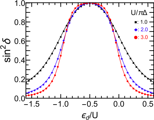
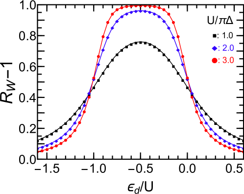
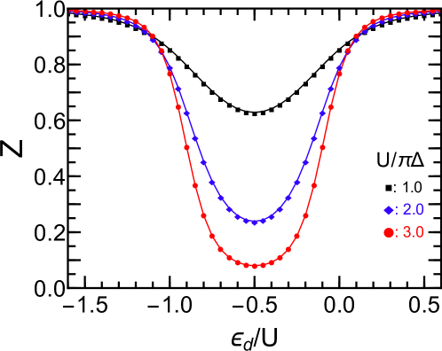
Figure 1: (Color online) NRG results of $\sin^{2}\delta$ ($=\pi\Delta\rho_{d})$, $R_{W}-1$, and $z$ at zero magnetic field $h=0$ are plotted vs $\epsilon_{d}/U$ for $U/(\pi\Delta)=1.0,2.0,$, and $3.0$.

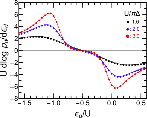
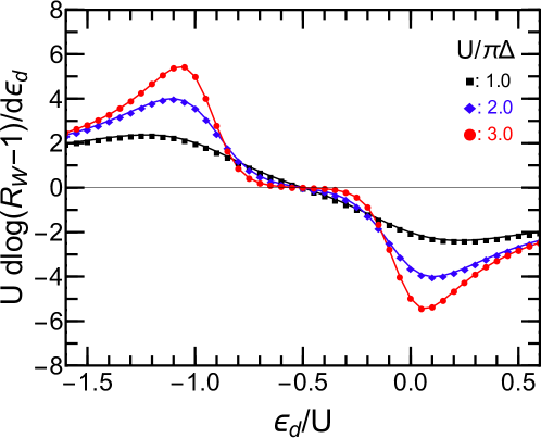
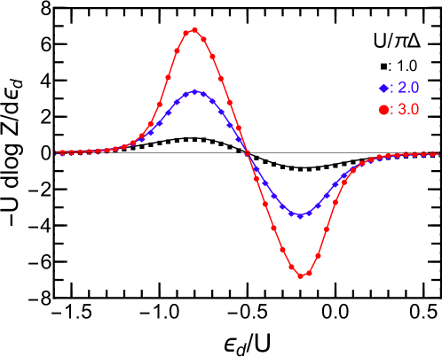
Figure 2: (Color online) Logarithmic derivatives of $\rho_{d}$ ($=\sin^{2}\delta/\pi\Delta$), $R_{W}-1$, and $z$ with respect to $\epsilon_{d}$ at zero magnetic field $h=0$ are plotted vs $\epsilon_{d}/U$ for $U/(\pi\Delta)=1.0,2.0,$, and $3.0$.

V Non-equilibrium transport through a quantum dot

We apply the low-energy asymptotic form of the self-energy obtained in the above to the non-equilibrium current $I$ through quantum dots.Glazman and Raikh (1988); Ng and Lee (1988); Hershfield et al. (1992); Wingreen and Meir (1994) The retarded Green’s function $G_{\sigma}^{r}(\omega,T,eV)$ and the spectral function $A_{\sigma}(\omega,T,eV)$ can be obtained from Eqs. (53) and (54):

$$\left\{G_{\sigma}^{r}(\omega,T,eV)\right\}^{-1}= \ \,\omega-\bigl{[}\,\epsilon_{d\sigma}+\mathrm{Re}\,\Sigma_{\sigma}^{r}(\omega,T,eV)\,\bigr{]}$$

$$+i\,\bigl{[}\,\Delta-\mathrm{Im}\,\Sigma_{\sigma}^{r}(\omega,T,eV)\,\bigr{]}\;,$$ (59)

$$A_{\sigma}(\omega,T,eV)\,\equiv \ -\frac{1}{\pi}\,\mathrm{Im}\,G_{\sigma}^{r}(\omega,T,eV)\;.$$ (60)

Note that $\rho_{d\sigma}(\omega)\equiv A_{\sigma}(\omega,0,0)$. Then, the current $I$ can be calculated using the Meir-Wingreen formula,Meir and Wingreen (1992); Hershfield et al. (1992)

$$I\,= \ \frac{e}{2\pi\hbar}\sum_{\sigma}\frac{4\Gamma_{L}\Gamma_{R}}{\Gamma_{L}+\Gamma_{R}}$$

$$\ \ \times\int_{-\infty}^{\infty}\!d\omega\,\bigl{[}\,f_{L}(\omega)-f_{R}(\omega)\,\bigr{]}\,\pi A_{\sigma}(\omega,T,eV).$$ (61)

Thus, $T$ and $eV$ enter through the distribution function $f_{L}-f_{R}$ and the spectral function $A_{\sigma}$.

V.1 Conductance formula for $\Gamma_{L}=\Gamma_{R}$ and $\alpha=0$

In the following, we consider the situation in which $\alpha=0$, taking the tunneling couplings and the bias voltages such that $\Gamma_{L}=\Gamma_{R}=\Delta/2$ and $\alpha_{L}=\alpha_{R}=1/2$. We obtain the spectral function up to terms of order $\omega^{2}$, $(eV)^{2}$, and $T^{2}$,

$$\pi\Delta\,A_{\sigma}(\omega,eV,T)\ =\ \sin^{2}\delta_{\sigma}+\pi\sin 2\delta_{\sigma}\,\chi_{\sigma\sigma}\ \omega$$

$$+\pi^{2}\left[\cos 2\delta_{\sigma}\left(\chi_{\sigma\sigma}^{2}+\frac{1}{2}\chi_{\uparrow\downarrow}^{2}\right)-\frac{\sin 2\delta_{\sigma}}{2\pi}\,\frac{\partial\chi_{\sigma\sigma}}{\partial\epsilon_{d\sigma}}\right]\omega^{2}$$

$$+\frac{\pi^{2}}{3}\!\left(\frac{3}{2}\cos 2\delta_{\sigma}\,\chi_{\uparrow\downarrow}^{2}-\frac{\sin 2\delta_{\sigma}}{2\pi}\frac{\partial\chi_{\uparrow\downarrow}}{\partial\epsilon_{d,-\sigma}}\right)\!\left[\frac{3}{4}\left(eV\right)^{2}\!+\left(\pi T\right)^{2}\right]$$

$$+\cdots.$$ (62)

The contribution of the non-linear fluctuation, $\partial\chi_{\uparrow\downarrow}/\partial\epsilon_{d,-\sigma}$, enters in the coefficient for $(\pi T)^{2}+(3/4)(eV)^{2}$ through Eq. (54). We calculate the current $I$ up to order $(eV)^{3}$ using Eqs. (61) and (62), and obtain the differential conductance,

$$\frac{dI}{dV}=\frac{e^{2}}{2\pi\hbar}\sum_{\sigma}\left[\sin^{2}\delta_{\sigma}-c_{T,\sigma}\left(\pi T\right)^{2}-c_{V,\sigma}\left(eV\right)^{2}+\cdots\right].$$ (63)

The coefficients $c_{T,\sigma}$ and $c_{V,\sigma}$ are given by

$$c_{T,\sigma}= \ \frac{\pi^{2}}{3}\Biggl{[}\,-\cos 2\delta_{\sigma}\left(\chi_{\sigma\sigma}^{2}+2\chi_{\uparrow\downarrow}^{2}\right)$$

$$\qquad\ +\,\frac{\sin 2\delta_{\sigma}}{2\pi}\,\left(\frac{\partial\chi_{\sigma\sigma}}{\partial\epsilon_{d\sigma}}+\frac{\partial\chi_{\uparrow\downarrow}}{\partial\epsilon_{d,-\sigma}}\right)\Biggr{]}\;,$$ (64)

$$c_{V,\sigma}= \ \frac{\pi^{2}}{4}\Biggl{[}\,-\cos 2\delta_{\sigma}\left(\chi_{\sigma\sigma}^{2}+5\,\chi_{\uparrow\downarrow}^{2}\right)$$

$$\qquad\ +\,\frac{\sin 2\delta_{\sigma}}{2\pi}\left(\,\frac{\partial\chi_{\sigma\sigma}}{\partial\epsilon_{d\sigma}}+3\,\frac{\partial\chi_{\uparrow\downarrow}}{\partial\epsilon_{d,-\sigma}}\right)\Biggr{]}\;.$$ (65)

We note that the derivatives, for which $\sin 2\delta_{\sigma}$ are multiplied, can be rewritten in terms of the derivatives with respect to $\epsilon_{d}$ and $h$,

$$\frac{\partial\chi_{\sigma\sigma}}{\partial\epsilon_{d\sigma}}+\frac{\partial\chi_{\uparrow\downarrow}}{\partial\epsilon_{d,-\sigma}}\,= \ \frac{\partial\chi_{\sigma\sigma}}{\partial\epsilon_{d}}+\sigma\frac{\partial\chi_{\uparrow\downarrow}}{\partial h}$$ (66)

$$\,\frac{\partial\chi_{\sigma\sigma}}{\partial\epsilon_{d\sigma}}\,+\,3\,\frac{\partial\chi_{\uparrow\downarrow}}{\partial\epsilon_{d,-\sigma}}\,= \ \frac{\partial\chi_{\sigma\sigma}}{\partial\epsilon_{d}}+\frac{\partial\chi_{\uparrow\downarrow}}{\partial\epsilon_{d}}\,+\,\sigma\,2\,\frac{\partial\chi_{\uparrow\downarrow}}{\partial h}.$$ (67)

In the particle-hole symmetric case at which $\epsilon_{d}=-U/2$ and $h=0$, the previous result is also reproducedOguri (2001)

$$\!\!\!\!\!c_{T,\sigma}\xrightarrow{h\to 0\atop\xi_{d}\to 0} \ \frac{\widetilde{\chi}_{\uparrow\uparrow}^{2}+2\widetilde{\chi}_{\uparrow\downarrow}^{2}}{3\Delta^{2}},\ \ c_{V,\sigma}\xrightarrow{h\to 0\atop\xi_{d}\to 0}\,\frac{\widetilde{\chi}_{\uparrow\uparrow}^{2}+5\widetilde{\chi}_{\uparrow\downarrow}^{2}}{4\Delta^{2}},\!\!$$ (68)

since $\delta_{\sigma}=\pi/2$ and $\rho_{d\sigma}=1/(\pi\Delta)$.

The last line of Eq. (64) and that of Eq. (65) are expressed in terms of the derivative with respect to the center of the impurity levels $\epsilon_{d}$ and the magnetic field $h$. We may also express these coefficients in a dimensionless way such that $c_{T,\sigma}(T^{*})^{2}$ and $c_{V,\sigma}(T^{*})^{2}$, scaling the quadratic $(\pi T)^{2}$ and $(eV)^{2}$ parts by the characteristic energy $T^{*}=1/4\sqrt{\chi_{\uparrow\uparrow}\chi_{\downarrow\downarrow}}{}$ that is introduced in Eq. (26b) and is a function of $\epsilon_{d}$ and $h$:

$$\frac{dI}{dV}= \ \frac{2e^{2}}{2\pi\hbar}\Biggl{[}\frac{1}{2}\sum_{\sigma}\sin^{2}\delta_{\sigma}$$

$$\qquad\ -C_{T}\left(\frac{\pi T}{T^{*}}\right)^{2}-C_{V}\left(\frac{eV}{T^{*}}\right)^{2}+\cdots\Biggr{]},$$ (69)

$$C_{T}\equiv \ \frac{(T^{*})^{2}}{2}\sum_{\sigma}\,c_{T,\sigma},\quad C_{V}\equiv\frac{(T^{*})^{2}}{2}\sum_{\sigma}\,c_{V,\sigma}.$$ (70)

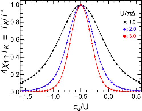
Figure 3: (Color online) Susceptibility $\chi_{\uparrow\uparrow}$ is plotted vs $\epsilon_{d}/U$ at zero magnetic field $h=0$. The reciprocal of it is proportional to the characteristic energy $T^{*}\equiv 1/4\chi_{\uparrow\uparrow}$. Here, the Kondo temperature $T_{K}\equiv z_{0}\pi\Delta/4$ is defined at half-filling $\epsilon_{d}/U=-0.5$ with the renormalization factor $z_{0}$ which depends on $U$: $z_{0}\simeq 0.63$, $0.24$, and $0.08$, for $U/\pi\Delta=1.0$, $2.0$, and $3.0$, respectively.

V.2 Conductance away from half-filling at zero field

The coefficients given in Eqs. (64) and (65) take a much simpler form at zero magnetic field $h=0$. Since ${\partial\chi_{\uparrow\downarrow}}/{\partial h}|_{h=0}=0$ as $\chi_{\uparrow\downarrow}$ is an even function of $h$, we obtain

$$c_{T,\sigma}\, \xrightarrow{\,h\to 0\,}\,\frac{\pi^{2}}{3}\left[\,-\left(\chi_{\uparrow\uparrow}^{2}+2\chi_{\uparrow\downarrow}^{2}\right)\cos 2\delta+\frac{\sin 2\delta}{2\pi}\,\frac{\partial\chi_{\uparrow\uparrow}}{\partial\epsilon_{d}}\,\right],$$ (71)

$$c_{V,\sigma}\, \xrightarrow{\,h\to 0\,}\,\frac{\pi^{2}}{4}\biggl{[}\,-\left(\chi_{\uparrow\uparrow}^{2}+5\,\chi_{\uparrow\downarrow}^{2}\right)\cos 2\delta$$

$$\qquad\qquad\qquad+\,\frac{\sin 2\delta}{2\pi}\left(\frac{\partial\chi_{\uparrow\uparrow}}{\partial\epsilon_{d}}+\frac{\partial\chi_{\uparrow\downarrow}}{\partial\epsilon_{d}}\right)\biggr{]}.$$ (72)

These coefficients $c_{T,\sigma}$ and $c_{V,\sigma}$ for $h=0$ coincide with those of FMvDM’s,Filippone et al. (2017) which were first presented in Ref.  Mora et al., 2015 by Mora, Moca, von Delft, and Zaránd (MMvDZ) away from half-filling at zero magnetic field.

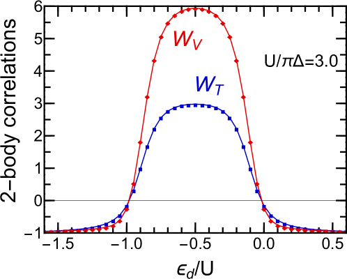
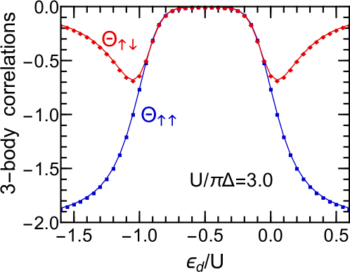
Figure 4: (Color online) Upper panel: contributions of the two-body fluctuations parts $W_{T}=-\left[1+2\left(R_{W}-1\right)^{2}\right]\cos 2\delta$, and $W_{V}=-\left[1+5\left(R_{W}-1\right)^{2}\right]\cos 2\delta$ are plotted vs $\epsilon_{d}$ for $U/\pi\Delta=3.0$ at $h=0$. Lower panel: contributions of the three-body fluctuations $\Theta_{\uparrow\uparrow}\equiv\frac{\sin 2\delta}{2\pi}\,\frac{1}{\chi_{\uparrow\uparrow}^{2}}\frac{\partial\chi_{\uparrow\uparrow}}{\partial\epsilon_{d}}$, and $\Theta_{\uparrow\downarrow}\equiv-\frac{\sin 2\delta}{2\pi}\,\frac{1}{\chi_{\uparrow\uparrow}^{2}}\frac{\partial\chi_{\uparrow\downarrow}}{\partial\epsilon_{d}}$. In the limit of $|\epsilon_{d}|\to\infty$, these parameters converge towards $W_{T}\to-1$, $W_{V}\to-1$, $\Theta_{\uparrow\uparrow}\to-2$, and $\Theta_{\uparrow\downarrow}\to 0$.

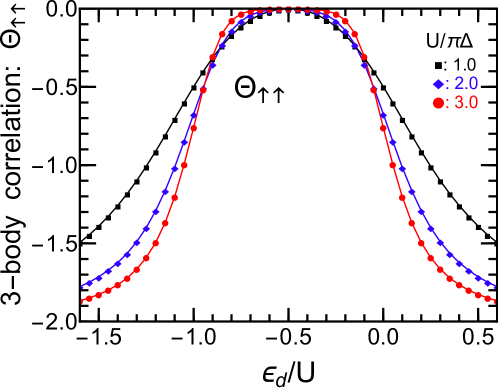
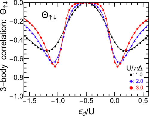
Figure 5: (Color online) Contributions of the three-body fluctuations $\Theta_{\uparrow\uparrow}$ and $\Theta_{\uparrow\downarrow}$ are plotted for several different values of $U/\pi\Delta$ ($=1.0,2.0$ and $3.0$). As $U$ increases, both of these two significantly vary at the crossover region from the Kondo regime to the empty (fully-occupied) orbital regime seen at $\epsilon_{d}/U\simeq 0.0$ ($\epsilon_{d}/U\simeq-1.0$).

Corresponding dimensionless parameters in this case are scaled by the characteristic energy $T^{*}=1/4\chi_{\uparrow\uparrow}$ which increases as $\epsilon_{d}$ deviates from the particle-hole symmetric point as shown in Fig. 3:

$$C_{T}\,= \ \frac{\pi^{2}}{48}\,\bigl{(}\,W_{T}\,+\,\Theta_{\uparrow\uparrow}\,\bigr{)}\;,$$ (73)

$$C_{V}\,= \ \frac{\pi^{2}}{64}\,\bigl{(}\,W_{V}\,+\,\Theta_{\uparrow\uparrow}-\Theta_{\uparrow\downarrow}\bigr{)}\;.$$ (74)

Here, $W_{T}$ and $W_{V}$ represents contributions of two-body fluctuations determined by the spin and charge susceptibilities, or the Wilson ratio $R_{W}$:

$$W_{T}\,= \ -\left[\,1+2\left(R_{W}-1\right)^{2}\,\right]\cos 2\delta\;,$$ (75)

$$W_{V}\,= \ -\left[\,1+5\left(R_{W}-1\right)^{2}\,\right]\cos 2\delta\;.$$ (76)

The other parts, $\Theta_{\uparrow\uparrow}$ and $\Theta_{\uparrow\downarrow}$, represent contributions of three-body fluctuations which can also be described in terms of the non-linear susceptibilities $\chi_{\sigma_{1}\sigma_{2}\sigma_{3}}^{[3]}$ defined in Eq. (15):

$$\Theta_{\uparrow\uparrow}\,\equiv \ \frac{\sin 2\delta}{2\pi}\,\frac{1}{\chi_{\uparrow\uparrow}^{2}}\frac{\partial\chi_{\uparrow\uparrow}}{\partial\epsilon_{d}}\;,$$ (77)

$$\Theta_{\uparrow\downarrow}\,\equiv \ -\frac{\sin 2\delta}{2\pi}\,\frac{1}{\chi_{\uparrow\uparrow}^{2}}\frac{\partial\chi_{\uparrow\downarrow}}{\partial\epsilon_{d}}\;.$$ (78)

At half-filling $\delta=\pi/2$, the Wilson ratio approaches $R_{W}\to 2$ for the Kondo regime $U\gtrsim 2\Delta$, and then $W_{T}\to 3$ and $W_{V}\to 6$, whereas the contribution of the three-body fluctuations vanish $\Theta_{\uparrow\uparrow}\to 0$ and $\Theta_{\uparrow\downarrow}\to 0$ as charge fluctuation is minimized and spin fluctuation is maximized.Yamada (1975a) We discuss in the following how the two-body and three-body contributions vary as $\epsilon_{d}$ deviates away from the particle-hole symmetric point.

The behavior in the other limit at $\epsilon_{d}\gg\max(U,\Delta)$ corresponds to the empty-orbital regime as already examined by MMvDZ.Mora et al. (2015) In the empty-orbital regime, the interaction can be neglected at low energies and thus for $\epsilon_{d}\to\infty$ the parameters asymptotically behave such that $R_{W}\to 1$, $\delta\simeq\Delta/\epsilon_{d}$, $\chi_{\uparrow\uparrow}\simeq\Delta/(\pi\epsilon_{d}^{2})$, and $\chi_{\uparrow\downarrow}\simeq 0$. Therefore,

$$\lim_{|\epsilon_{d}|\to\infty}W_{T}\,=\,-1,\qquad\lim_{|\epsilon_{d}|\to\infty}W_{V}\,=\,-1,$$ (79)

$$\lim_{|\epsilon_{d}|\to\infty}\Theta_{\uparrow\uparrow}\,=\,-2,\qquad\lim_{|\epsilon_{d}|\to\infty}\Theta_{\uparrow\downarrow}\,=\,0.$$ (80)

The opposite limit $\epsilon_{d}\to-\infty$, corresponding to a fully-filled orbital, links to the empty-orbital regime through the particle-hole transformation. The behavior of the two-body-fluctuation and three-body-fluctuation parts at intermediate $\epsilon_{d}$ can be explored using the NRG. Figure 4 shows a typical result obtained for $U=3\pi\Delta$. We see in the right panel explicitly the contributions of the three-body fluctuation, $\Theta_{\uparrow\uparrow}$ and $\Theta_{\uparrow\downarrow}$, are suppressed in the Kondo regime $-1.0\lesssim\epsilon_{d}/U\lesssim 0.0$. It also shows that the three-body fluctuations become important outside the Kondo regime. The anti-parallel component $\Theta_{\uparrow\downarrow}$ shows a minimum in the valence fluctuation region near $\epsilon_{d}/U\simeq-1.0$ and $0.0$, whereas the parallel component $\Theta_{\uparrow\uparrow}$ does not have an extremal point. Figure 5 shows the three-body contributions for several values of the interaction; $U/\pi\Delta=1.0,2.0$ and $3.0$. The crossover between the Kondo and empty (or fully-occupied) orbital regimes becomes sharp as $U$ increases, and correspondingly the transient region becomes very narrow for large $U$. The dependence of $C_{T}$ and $C_{V}$ on $\epsilon_{d}$ was already discussed by MMvDZ.Mora et al. (2015) We also provide similar results in Fig. 6 in order to explicitly show how the sum of two-body and three-body fluctuations determines these coefficients. The contributions of the two-body fluctuations which enter through $W_{T}$ and $W_{V}$ dominate in the Kondo regime, whereas the three-body fluctuation give significant contributions for $|\epsilon_{d}+U/2|\gtrsim U/2$. In the $|\epsilon_{d}|\to\infty$ limit of the empty (or fully-occupied) orbital regime, the coefficients converge towards $(48/\pi^{2})C_{T}\to-3$ and $(64/\pi^{2})C_{V}\to-3$,Mora et al. (2015) while those in the Kondo regime are given by $(48/\pi^{2})C_{T}\to 3$ and $(64/\pi^{2})C_{V}\to 6$ for $U\gtrsim 2\pi\Delta$.

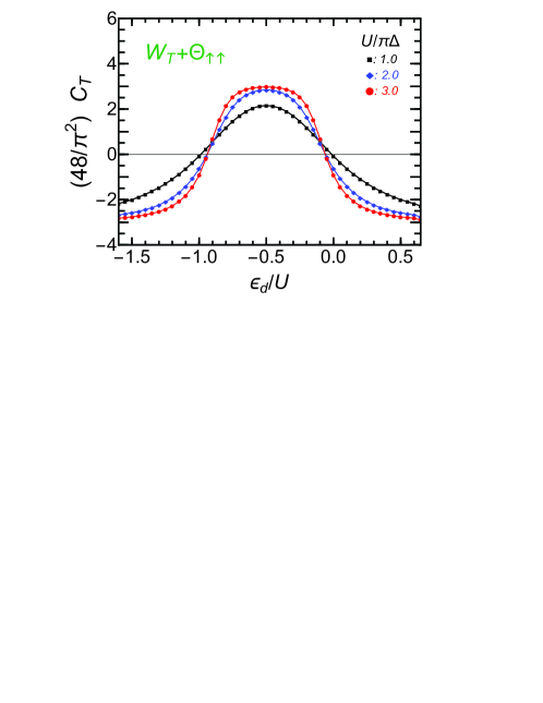
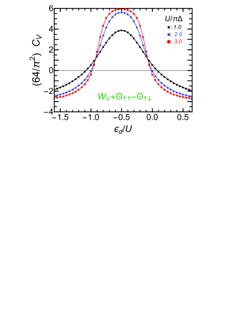
Figure 6: (Color online) Dimensionless coefficients $C_{T}$ and $C_{V}$ are plotted vs $\epsilon_{d}/U$ for $U/\pi\Delta=1.0$, $2.0$, and $3.0$ at $h=0$. Note that numerical factor has been introduced such that $(48/\pi^{2})\,C_{T}=W_{T}+\Theta_{\uparrow\uparrow}$ and $(64/\pi^{2})\,C_{V}=W_{V}+\Theta_{\uparrow\uparrow}-\Theta_{\uparrow\downarrow}$.

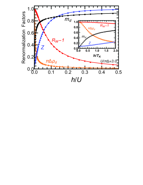
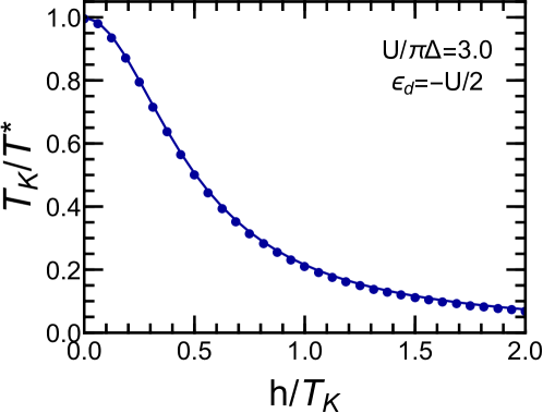
Figure 7: (Color online) Magnetic field dependence of Fermi-liquid parameters at half-filling $\epsilon_{d}=-U/2$ for $U/\pi\Delta=3.0$ plotted vs $h/U$. Inset shows an enlarged view of a small $h$ region, for which the horizontal axis is scaled by $T_{K}=0.02\pi\Delta$ determined at $h=0$. Upper panel shows $Z$, $R_{W}-1$, $\pi\Delta\rho_{d}=\cos^{2}(\pi m_{d}/2)$, and $m_{d}\equiv n_{d\uparrow}-n_{d\downarrow}$. Using this definition of $T_{K}$, the reciprocal of the field-dependent characteristic energy $T^{*}$ is plotted vs $h/T_{K}$ in the right panel.

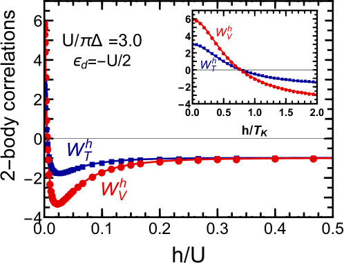
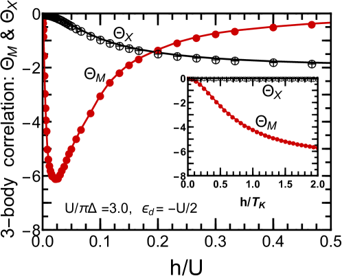
Figure 8: (Color online) Two-body and three-body correlations which determine $C_{T}^{h}$ and $C_{V}^{h}$ are plotted vs $h/U$ at half-filling $\epsilon_{d}=-U/2$ for $U/\pi\Delta=3.0$. Inset shows an enlarged view of the small $h$ region, for which the horizontal axis is scaled by $T_{K}=0.02\pi\Delta$ ($=0.0066U$) determined at $h=0$. Upper panel shows the contribution of two-body fluctuations $W_{T}^{h}=\left[1+2\left(R_{W}-1\right)^{2}\right]\cos(\pi m_{d})$, and $W_{V}^{h}=\left[1+5\left(R_{W}-1\right)^{2}\right]\cos(\pi m_{d})$. Lower panel shows the contribution of three-body fluctuations $\Theta_{M}$ and $\Theta_{X}$, defined in Eqs. (86a) and (86b).

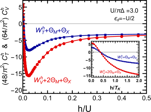
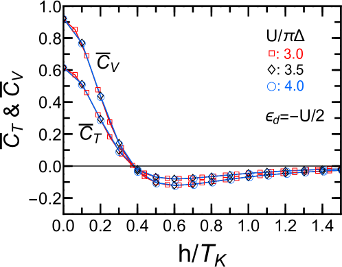
Figure 9: (Color online) Magnetic-field dependence of the $dI/dV$ coefficients: Upper panel shows $(48/\pi^{2})\,C_{T}^{h}=W_{T}^{h}+\Theta_{M}+\Theta_{X}$ and $(64/\pi^{2})\,C_{V}^{h}=W_{V}^{h}+2\Theta_{M}+\Theta_{X}$. Inset describes an enlarged view of the small $h$ region. Lower panel shows rescaled coefficients $\overline{C}_{T}=(T_{K}/T^{*})^{2}C_{T}^{h}$ and $\overline{C}_{V}=(T_{K}/T^{*})^{2}C_{V}^{h}$ defined in Eq. (90), using the $h$-independent $T_{K}$. The Kondo temperature $T_{K}=z_{0}\pi\Delta/4$ is determined at $h=0$ with the renormalization factor $z_{0}\simeq 0.08$, $0.05$, and $0.03$ for $U/\pi\Delta=3.0$, $3.5$, and $4.0$, respectively

V.3 Conductance at finite magnetic fields for $\epsilon_{d}=-U/2$

We next consider the conductance at finite magnetic fields $h\neq 0$, applied at half-filling $\xi_{d}=0$. In this case, the average of total occupation number for both spin components is fixed at $n_{d\uparrow}+n_{d\downarrow}=1$, and thus the phase shift for each spin component can be expressed in the form $\delta_{\sigma}=\pi(1+\sigma m_{d})/2$, with $m_{d}=n_{d\uparrow}-n_{d\downarrow}$ the induced magnetization. Furthermore, since $\rho_{d\uparrow}=\rho_{d\downarrow}$, $\chi_{\uparrow\uparrow}=\chi_{\downarrow\downarrow}$, $z_{\uparrow}=z_{\downarrow}$($\equiv z$), and the coefficients for the $T^{2}$ and $(eV)^{2}$ terms defined in Eqs. (64) and (65) are simplified,

$$\frac{1}{2}\sum_{\sigma}c_{T,\sigma}$$

$$\xrightarrow{\xi_{d}\to 0}\frac{\pi^{2}}{3}\Biggl{[}\left(\chi_{\uparrow\uparrow}^{2}+2\chi_{\uparrow\downarrow}^{2}\right)\cos(\pi m_{d})-\frac{\sin(\pi m_{d})}{2\pi}\frac{\partial\chi_{\uparrow\downarrow}}{\partial h}$$

$$\qquad\qquad\quad-\,\frac{\sin(\pi m_{d})}{2\pi}\frac{\partial}{\partial\epsilon_{d}}\left(\frac{\chi_{\uparrow\uparrow}-\chi_{\downarrow\downarrow}}{2}\right)\Biggr{]},$$ (81)

$$\frac{1}{2}\sum_{\sigma}c_{V,\sigma}$$

$$\xrightarrow{\xi_{d}\to 0}\frac{\pi^{2}}{4}\Biggl{[}\left(\chi_{\uparrow\uparrow}^{2}+5\,\chi_{\uparrow\downarrow}^{2}\right)\cos(\pi m_{d})-\frac{\sin(\pi m_{d})}{\pi}\,\frac{\partial\chi_{\uparrow\downarrow}}{\partial h}$$

$$\qquad\qquad\quad-\,\frac{\sin(\pi m_{d})}{2\pi}\frac{\partial}{\partial\epsilon_{d}}\left(\frac{\chi_{\uparrow\uparrow}-\chi_{\downarrow\downarrow}}{2}\right)\Biggr{]}.$$ (82)

The three-body contribution that enters through $\partial\chi_{\uparrow\downarrow}/\partial\epsilon_{d}$ has vanished because the contributions of $\uparrow$ and $\downarrow$ spin components cancel each other out. The characteristic energy $T^{*}=1/4\chi_{\uparrow\uparrow}$ in the present case depends on $h$ as shown in Fig. 7.

Multiplying Eqs. (81)–(82) by $(T^{*})^{2}$, we obtain the dimensionless coefficients

$$C_{T}^{h}\equiv \ \frac{\pi^{2}}{48}\left(W_{T}^{h}+\Theta_{M}+\Theta_{X}\right),$$ (83a)

$$C_{V}^{h}\equiv \ \frac{\pi^{2}}{64}\left(W_{V}^{h}+2\Theta_{M}+\Theta_{X}\right).\!$$ (83b)

Here, $W_{T}^{h}$ and $W_{V}^{h}$ represent contributions of the two-body fluctuations,

$$W_{T}^{h}\,\equiv \ \left[\,1+2\left(R_{W}-1\right)^{2}\,\right]\cos(\pi m_{d}),$$ (84)

$$W_{V}^{h}\,\equiv \ \left[\,1+5\left(R_{W}-1\right)^{2}\,\right]\cos(\pi m_{d}).$$ (85)

The remaining contribution of the three-body fluctuations are described by $\Theta_{M}$ and $\Theta_{X}$,

$$\Theta_{M}\,\equiv \ -\,\frac{\sin(\pi m_{d})}{2\pi}\frac{1}{\chi_{\uparrow\uparrow}^{2}}\,\frac{\partial\chi_{\uparrow\downarrow}}{\partial h}\,,$$ (86a)

$$\Theta_{X}\,\equiv \ -\,\frac{\sin(\pi m_{d})}{2\pi}\frac{1}{\chi_{\uparrow\uparrow}^{2}}\frac{\partial}{\partial\epsilon_{d}}\left(\frac{\chi_{\uparrow\uparrow}-\chi_{\downarrow\downarrow}}{2}\right)\;.$$ (86b)

The contribution of this three-body correlation at finite magnetic fields can also be decomposed into the logarithmic derivatives of the renormalization factor and the Wilson ratio, similarly to Eqs. (57) and (58),

$$\frac{\partial\log(-\chi_{\uparrow\downarrow})}{\partial h}\,=\,\frac{\partial\log\chi_{\uparrow\uparrow}}{\partial h}+\frac{\partial\log(R_{W}-1)}{\partial h},$$ (87)

$$\frac{\partial\log\chi_{\uparrow\uparrow}}{\partial h}=-\frac{\partial\log z}{\partial h}-2\pi R_{W}\,\chi_{\uparrow\uparrow}\tan\left(\frac{\pi m_{d}}{2}\right).$$ (88)

Figure 7 shows the magnetic-field dependence of the renormalized parameters, obtained with the NRG.Hewson et al. (2004) It indicates that the induced magnetization $m_{d}$ and the density of states $\sin^{2}\delta=\pi\Delta\rho_{\sigma}$ rapidly vary at small fields $h\lesssim T_{K}$ as the Kondo resonance goes away from the Fermi level. In contrast, the wavefunction renormalization factor $z$ and $R_{W}$ vary more slowly than $m_{d}$ and $\sin^{2}\delta_{\sigma}$ with the energy scale of the Coulomb interaction $U$. Figure 8 shows the magnetic-field dependence of the contributions of two-body fluctuations and three-body fluctuations on the coefficients $C_{T}^{h}$ and $C_{V}^{h}$. The two-body correlations are given by $W_{T}^{h}=3$ and $W_{T}^{h}=6$ at zero field for large interactions ($U\gtrsim 2\pi\Delta$) as $m_{d}=0$ and $R_{W}\to 2$. As $h$ increases, these two-body contributions change sign near $h=0.8T_{K}$ with $T_{K}=0.02\pi\Delta=0.0066U$ that is determined at $h=0$ for $U=3.0\pi\Delta$. Both of these two correlations show a minimum near $h\simeq 0.02U$, and then approach $\lim_{h\to\infty}W_{T}^{h}=-2$ and $\lim_{h\to\infty}W_{V}^{h}=-2$ for large magnetic fields where $m_{d}\to 1$ and $R_{W}\to 1$. The three-body contribution $\Theta_{M}$ vanishes at $h=0$, and in the large-field limit $\lim_{|h|\to\infty}\Theta_{M}=0$ as $\chi_{\uparrow\downarrow}$ decreases faster than $\chi_{\uparrow\uparrow}$. It also has a deep minimum of $\Theta_{M}\simeq-6.0$, which is deeper than that of $W_{V}^{h}\simeq-3.7$, at an intermediate field $h\simeq 0.02U$ for the case $U=3.0\pi\Delta$. We also see that $\Theta_{M}$ gives a comparable contribution with that of $W_{T}^{h}$ and $W_{V}^{h}$ at small fields $h\lesssim T_{K}$. The other three-body term $\Theta_{X}$ also vanishes at $h=0$, and at $h\lesssim T_{K}$ it takes a very small negative value and does not contribute to $C_{T}^{h}$ and $C_{V}^{h}$ very much. However, it becomes comparable to $\Theta_{M}$ at high fields $h\gtrsim 0.1U$, and then approaches $\lim_{|h|\to\infty}\Theta_{X}=-2$ which corresponds to the value in the noninteracting case.

The lower panel of Fig. 9 shows the total contributions: $(48/\pi^{2})\,C_{T}^{h}=W_{T}^{h}+\Theta_{M}+\Theta_{X}$, and $(64/\pi^{2})\,C_{V}^{h}=W_{V}^{h}+2\Theta_{M}+\Theta_{X}$ for the same interaction $U=3.0\pi\Delta$. For $h\gtrsim 0.8T_{K}=0.0053U$, both the two-body and three-body correlations give negative contributions, and thus the minimum of $C_{T}^{h}$ and also that of $C_{V}^{h}$ become deeper than the minimum of the individual contributions alone. It indicates that the three-body correlation $\Theta_{M}$ dominates the contribution on the $T^{2}$ and $(eV)^{2}$ part of $dI/dV$ near the minimum $0.01U\lesssim h\lesssim 0.1U$. So far, we have used the field-dependent energy $T^{*}$ to scale the $T^{2}$ and $(eV)^{2}$ dependences. In order to examine the universal Kondo-scaling behavior for small magnetic fields, however, we use $T_{K}$ determined at $h=0$ as an $h$-independent characteristic energy and rescale $dI/dV$ such that

$$\frac{dI}{dV}= \ \frac{2e^{2}}{2\pi\hbar}\Biggl{[}\,\frac{1}{2}\sum_{\sigma}\sin^{2}\delta_{\sigma}$$

$$\qquad-\overline{C}_{T}\left(\frac{\pi T}{T_{K}}\right)^{2}-\overline{C}_{V}\left(\frac{eV}{T_{K}}\right)^{2}+\cdots\Biggr{]},$$ (89)

$$\overline{C}_{T}\,\equiv \ \left(\frac{T_{K}}{T^{*}}\right)^{2}C_{T}^{h}\,,\qquad\overline{C}_{V}\,\equiv\,\left(\frac{T_{K}}{T^{*}}\right)^{2}C_{K}^{h}.$$ (90)

In the right panel of Fig.  9, $\overline{C}_{T}$ and $\overline{C}_{V}$ are plotted vs $h/T_{K}$, using $T_{K}$ for each $U/\pi\Delta=3.0,3.5,4.0$. We see that both the coefficients $\overline{C}_{T}$ and $\overline{C}_{V}$ show universal Kondo behavior. This is mainly caused by the fact that the Wilson ratio is almost saturated $R_{W}\simeq 2$ for strong interactions $U$. These two coefficients, $\overline{C}_{T}$ and $\overline{C}_{V}$, also show a similar $h$ dependence, especially they both change sign at finite magnetic field $h\simeq 0.38T_{K}$ of the order of the Kondo temperature. Therefore, the zero-bias peak of the conductance splits for large magnetic fields $h\gtrsim 0.38T_{K}$ as $dI/dV$ increases from the zero-bias value as $eV$ or $T$ increases.Hewson et al. (2006) These observations are also consistent with the result of the second-order renormalized perturbation theory. Hewson et al. (2006, 2005)

VI Thermoelectric transport of dilute magnetic alloy

The Kondo effect in dilute magnetic alloy (MA) has been studied for a wide variety of $3d$, $4f$, and $5f$ electron systems. Our formulation can also be applied to these original Kondo systems. In this subsection, we provide the microscopic description of the Fermi-liquid corrections for magneto-transport properties of dilute magnetic alloys away from half-filling. Specifically, we calculate the electric resistance $R_{\mathrm{MA}}$, thermoelectric power $S$, and thermal conductivity $\kappa$ using the linear-response formulas,Costi et al. (1994); Oguri and Maekawa (1990)

$$\frac{1}{R_{\mathrm{MA}}}= \ \frac{1}{2R_{\mathrm{MA}}^{0}}\sum_{\sigma}\mathcal{L}_{0,\sigma}\,,\quad\ \ \mathcal{S}\,=\,\frac{-1}{|e|T}\frac{\sum_{\sigma}\mathcal{L}_{1,\sigma}}{\sum_{\sigma}\mathcal{L}_{0,\sigma}}\,,$$ (91)

$$\kappa\,= \ \frac{\eta_{0}}{T}\left(\sum_{\sigma}\mathcal{L}_{2,\sigma}-\frac{\left(\sum_{\sigma}\mathcal{L}_{1,\sigma}\right)^{2}}{\sum_{\sigma}\mathcal{L}_{0,\sigma}}\right).$$ (92)

The coefficients are defined by

$$\mathcal{L}_{n,\sigma}=\int_{-\infty}^{\infty}d\omega\,\frac{\omega^{n}}{\pi\Delta A_{\sigma}(\omega,T)}\left(-\frac{\partial f(\omega)}{\partial\omega}\right).$$ (93)

The factor $R_{\mathrm{MA}}^{0}$ is the unitary-limit value of the electric resistance at zero field. Similarly, $\eta_{0}$ is defined such that the $T$-linear thermal conductivity should take the following form in the unitary limit,

$$\kappa_{0}=\frac{2\pi^{2}\eta_{0}}{3}\,T\;.$$ (94)

Note that thermoelectric transport through quantum dots can also be determined in a similar wayGuttman et al. (1995).

VI.1 Coefficients $\mathcal{L}_{n,\sigma}$ for finite magnetic fields

The coefficients $\mathcal{L}_{n,\sigma}$, defined in Eqs. (93), are written in terms of the inverse spectral function which physically represents the relaxation time due to the many-body scattering by the impurity at equilibrium $eV=0$. For this spectral function, we use the low-energy asymptotic form given in Eq. (62),

$$\frac{A_{\sigma}(0,0,0)}{A_{\sigma}(\omega,T,eV=0)}\,$$

$$= \ 1-\frac{\pi}{3\Delta\rho_{d\sigma}}\left(\frac{3}{2}\cos 2\delta_{\sigma}\,\chi_{\uparrow\downarrow}^{2}-\frac{\sin 2\delta_{\sigma}}{2\pi}\,\frac{\partial\chi_{\uparrow\downarrow}}{\partial\epsilon_{d,-\sigma}}\right)\left(\pi T\right)^{2}$$

$$-\frac{\sin 2\delta_{\sigma}\,\chi_{\sigma\sigma}}{\Delta\rho_{d\sigma}}\,\omega+\frac{\pi}{\Delta\rho_{d\sigma}}\Biggl{[}\bigl{(}2+\cos 2\delta_{\sigma}\bigr{)}\,\chi_{\sigma\sigma}^{2}$$

$$-\frac{1}{2}\cos 2\delta_{\sigma}\chi_{\uparrow\downarrow}^{2}+\frac{\sin 2\delta_{\sigma}}{2\pi}\,\frac{\partial\chi_{\sigma\sigma}}{\partial\epsilon_{d\sigma}}\Biggr{]}\,\omega^{2}+\cdots.$$ (95)

Note that $\pi\Delta\rho_{d\sigma}=\sin^{2}\delta_{\sigma}$. Using also the integration formulas,

$$\int_{-\infty}^{\infty}d\omega\,\omega^{2}\left(-\frac{\partial f(\omega)}{\partial\omega}\right)= \ \frac{1}{3}\,(\pi T)^{2},$$ (96a)

$$\int_{-\infty}^{\infty}d\omega\,\omega^{4}\left(-\frac{\partial f(\omega)}{\partial\omega}\right)= \ \frac{7}{15}\,(\pi T)^{4}\;,$$ (96b)

we obtain $\mathcal{L}_{n,\sigma}$ for $n=0,1,$ and $2$:

$$\mathcal{L}_{0,\sigma}=\frac{1}{\pi\Delta\rho_{d\sigma}}\Biggl{[}1+\frac{\pi}{3\Delta\,\rho_{d\sigma}}\biggl{\{}\bigl{(}2+\cos 2\delta_{\sigma}\bigr{)}\,\chi_{\sigma\sigma}^{2}$$

$$\quad-2\cos 2\delta_{\sigma}\,\chi_{\uparrow\downarrow}^{2}+\frac{\sin 2\delta_{\sigma}}{2\pi}\,\left(\frac{\partial\chi_{\sigma\sigma}}{\partial\epsilon_{d\sigma}}+\frac{\partial\chi_{\uparrow\downarrow}}{\partial\epsilon_{d,-\sigma}}\right)\,\biggr{\}}\left(\pi T\right)^{2}\Biggr{]}$$

$$\quad+O(T^{4}),$$ (97)

$$\mathcal{L}_{1,\sigma}=-\frac{2\pi}{3}\frac{\cot\delta_{\sigma}}{\pi\Delta\rho_{d\sigma}}\,\chi_{\sigma\sigma}\,(\pi T)^{2}+O(T^{4})\;,$$ (98)

$$\mathcal{L}_{2,\sigma}=\frac{\left(\pi T\right)^{2}}{3\pi\Delta\rho_{d\sigma}}\Biggl{[}1+\frac{7\pi}{5\Delta\rho_{d\sigma}}\biggl{\{}\bigl{(}2+\cos 2\delta_{\sigma}\bigr{)}\,\chi_{\sigma\sigma}^{2}$$

$$\quad-\frac{6}{7}\cos 2\delta_{\sigma}\chi_{\uparrow\downarrow}^{2}+\frac{\sin 2\delta_{\sigma}}{2\pi}\left(\frac{\partial\chi_{\sigma\sigma}}{\partial\epsilon_{d\sigma}}+\frac{5}{21}\frac{\partial\chi_{\uparrow\downarrow}}{\partial\epsilon_{d,-\sigma}}\right)\biggr{\}}\left(\pi T\right)^{2}\Biggr{]}$$

$$\quad+O(T^{6}).$$ (99)

The derivatives in the last part of $\mathcal{L}_{2,\sigma}$ can also be written as

$$\frac{\partial\chi_{\sigma\sigma}}{\partial\epsilon_{d\sigma}}+\frac{5}{21}\frac{\partial\chi_{\uparrow\downarrow}}{\partial\epsilon_{d,-\sigma}}=\frac{\partial\chi_{\sigma\sigma}}{\partial\epsilon_{d}}-\frac{8}{21}\frac{\partial\chi_{\uparrow\downarrow}}{\partial\epsilon_{d}}+\sigma\,\frac{13}{21}\frac{\partial\chi_{\uparrow\downarrow}}{\partial h}.$$ (100)

The asymptotic exact low-temperature form of the transport coefficients $R_{\mathrm{MA}}$, $S$, and $\kappa$ for finite magnetic fields can be explicitly written down using Eqs. (97)–(99) for Eq. (92). As those general Fermi-liquid expressions become rather lengthy for $h\neq 0$, we explicitly write in the following the transport coefficients of dilute magnetic alloys at zero magnetic field.

VI.2 Thermoelectric transport coefficients at zero magnetic field

The electric resistance takes the following form at zero magnetic field $h=0$ away from half-filling,

$$\frac{R_{\mathrm{MA}}}{{R_{\mathrm{MA}}^{0}}}\,=\,\sin^{2}\delta-c_{R}^{\mathrm{MA}}\left(\pi T\right)^{2}+O(T^{4})\;,$$ (101)

$$c_{R}^{\mathrm{MA}}=\frac{\pi^{2}}{3}\left[\bigl{(}2+\cos 2\delta\bigr{)}\,\chi_{\uparrow\uparrow}^{2}-2\cos 2\delta\,\chi_{\uparrow\downarrow}^{2}+\frac{\sin 2\delta}{2\pi}\,\frac{\partial\chi_{\uparrow\uparrow}}{\partial\epsilon_{d}}\right].$$ (102)

Note that it reproduces the results of Yamada-Yosida in the particle-hole symmetric case, Yamada (1975a, b)

$$\frac{R_{\mathrm{MA}}}{{R_{\mathrm{MA}}^{0}}}\,\xrightarrow{\,\xi_{d}\to 0\,} \ 1\,-\,\frac{\widetilde{\chi}_{\uparrow\uparrow}^{2}+2\widetilde{\chi}_{\uparrow\downarrow}^{2}}{3}\left(\frac{\pi T}{\Delta}\right)^{2}+O(T^{4})\;.$$ (103)

We introduce the dimensionless coefficient $C_{R}^{\mathrm{MA}}$ which is scaled by $T^{*}=1/(4\chi_{\uparrow\uparrow})$, the characteristic energy at $h=0$;

$$C_{R}^{\mathrm{MA}}\,\equiv \ c_{R}^{\mathrm{MA}}(T^{*})^{2}\,=\,\frac{\pi^{2}}{48}\left(\,W_{R}^{\mathrm{MA}}\,+\,\Theta_{\uparrow\uparrow}\right)\;,$$ (104)

$$W_{R}^{\mathrm{MA}}\,\equiv \ 2+\cos 2\delta-2\left(R_{W}-1\right)^{2}\cos 2\delta\;.$$ (105)

Here, $W_{R}^{\mathrm{MA}}$ represents the contribution of the two-body fluctuation, and $\Theta_{\uparrow\uparrow}$ which is defined in Eq. (77) represents the contribution of three-body fluctuations. The coefficient $C_{R}^{\mathrm{MA}}$ does not depend on the anti-parallel component of three-body correlation $\Theta_{\uparrow\downarrow}$ similarly to the coefficient $C_{T}$ for quantum dots given in Eq. (73).

In our formulation, low-temperature expansion of the thermopower $S$ can be carried out just for the leading $T$-linear term. It is determined by the derivative of the density of states at the Fermi energy $\omega=0$, and can be written in the following form at zero magnetic field,

$$\mathcal{S}\,= \ \frac{\pi^{2}}{3}\,\frac{\rho_{d}^{\prime}}{\rho_{d}}\,\frac{T}{|e|}\ +O(T^{3})\;.$$ (106)

Here $\rho_{d}^{\prime}$ is the derivative with respect to $\omega$, defined in Eq, (21).

Figure 10: (Color online) Contributions of the two-body fluctuation parts $W_{R}^{\mathrm{MA}}$ and $W_{\kappa}^{\mathrm{MA}}$, defined in Eqs. (105) and (113), are plotted vs $\epsilon_{d}/U$ for $U=3.0\pi\Delta$.

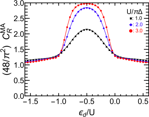
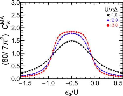
Figure 11: (Color online) Coefficients $C_{R}^{\mathrm{MA}}$ and $C_{\kappa}^{\mathrm{MA}}$, defined in Eqs. (104) and (112), for the electric resistance and thermal conductivity are plotted vs $\epsilon_{d}/U$ for $U/\pi\Delta=1.0$, $2.0$, and $3.0$. These coefficients converge towards $(48/\pi^{2})\,C_{R}^{\mathrm{MA}}\to 1$ and $(80/7\pi^{2})\,C_{\kappa}^{\mathrm{MA}}\to 1/21$ for $|\epsilon_{d}|\to\infty$.

The thermal conductivity $\kappa$ can be deduced up terms of order $T^{3}$ through Eq. (92). At $h=0$, the leading $T^{4}$ term of the ratio $(\sum_{\sigma}\mathcal{L}_{1,\sigma})^{2}/\sum_{\sigma}\mathcal{L}_{0,\sigma}$ is given by

$$\frac{\left(\sum_{\sigma}\mathcal{L}_{1,\sigma}\right)^{2}}{\sum_{\sigma}\mathcal{L}_{0,\sigma}}\,=\,\frac{8\pi^{2}}{9}\cot^{2}\delta\,\chi_{\uparrow\uparrow}^{2}\,\frac{(\pi T)^{4}}{\pi\Delta\rho_{d}}\,+O(T^{6})\;.$$ (107)

Using this ratio and $\mathcal{L}_{2,\sigma}$ given in Eq. (99), we can explicitly write the thermal conductivity at zero magnetic field,

$$\kappa\,= \ \frac{2\pi^{2}\eta_{0}}{3}\frac{T}{\sin^{2}\delta}\,\left[\,1+\frac{c_{\kappa}^{\mathrm{MA}}}{\sin^{2}\delta}\,\left(\pi T\right)^{2}\,\right]+O(T^{5})\,,$$ (108)

$$c_{\kappa}^{\mathrm{MA}}\,\equiv \ \frac{7\pi^{2}}{5}\biggl{[}\,\frac{32+11\cos 2\delta}{21}\,\chi_{\uparrow\uparrow}^{2}-\frac{6}{7}\cos 2\delta\,\chi_{\uparrow\downarrow}^{2}$$

$$\qquad\quad+\frac{\sin 2\delta}{2\pi}\left(\frac{\partial\chi_{\uparrow\uparrow}}{\partial\epsilon_{d}}-\frac{8}{21}\,\frac{\partial\chi_{\uparrow\downarrow}}{\partial\epsilon_{d}}\right)\,\biggr{]}.$$ (109)

Here, the sign and normalization of $c_{\kappa}^{\mathrm{MA}}$ has been determined in such a way that the thermal resistivity, the reciprocal of $\kappa$, is written in the following form,

$$\frac{1}{\kappa}\,= \ \frac{3}{2\pi^{2}\eta_{0}T}\left[\,\sin^{2}\delta\,-\,c_{\kappa}^{\mathrm{MA}}\,\left(\pi T\right)^{2}\,\right]+O(T^{3})\,.$$ (110)

In the particle-hole symmetric case, Eq. (109) reproduces the expression that can be deduced from the result of Yamada-Yosida,

$$\kappa\,\xrightarrow{\,\xi_{d}\to 0\,} \ \frac{2\pi^{2}\eta_{0}}{3}\,T\,\Biggl{[}1+\frac{7\widetilde{\chi}_{\uparrow\uparrow}^{2}+6\,\widetilde{\chi}_{\uparrow\downarrow}^{2}}{5}\left(\frac{\pi T}{\Delta}\right)^{2}\Biggr{]}+O(T^{5})\,.$$ (111)

We also introduce the dimensionless coefficient in the same way as that for the coefficient $C_{R}^{\mathrm{MA}}$ of the electric resistance

$$\!\!\!\!\!C_{\kappa}^{\mathrm{MA}}\equiv c_{\kappa}^{\mathrm{MA}}(T^{*})^{2}\!=\frac{7\pi^{2}}{80}\left(\!W_{\kappa}^{\mathrm{MA}}+\Theta_{\uparrow\uparrow}\!+\frac{8}{21}\Theta_{\uparrow\downarrow}\!\right)\!,\!\!$$ (112)

$$\!\!\!\!W_{\kappa}^{\mathrm{MA}}\,\equiv\,\frac{32+11\cos 2\delta}{21}\,-\frac{6}{7}\left(R_{W}-1\right)^{2}\cos 2\delta.$$ (113)

Both the parallel and anti-parallel components of the three-body fluctuation, $\Theta_{\uparrow\uparrow}$ and $\Theta_{\uparrow\downarrow}$ contribute to the thermal conductivity. The dependence of these three-body correlation functions on $\epsilon_{d}$ has been shown in Figs. 4 and 5.

We also show the $\epsilon_{d}$ dependence of the two-body-fluctuation part of the electric resistance and the thermal conductivity, $W_{R}^{\mathrm{MA}}$ and $W_{\kappa}^{\mathrm{MA}}$, in Fig.  10 for $U=3.0\pi\Delta$. The contributions of the two-body fluctuation reach the unitary-limit value $W_{R}^{\mathrm{MA}}\xrightarrow{\mathrm{Kondo}}3$ and $W_{\kappa}^{\mathrm{MA}}\xrightarrow{\mathrm{Kondo}}13/7$ in the Kondo regime where $\delta\to\pi/2$ and $R_{W}\to 2$. Both $W_{R}^{\mathrm{MA}}$ and $W_{\kappa}^{\mathrm{MA}}$ do not change sign in contrast to $W_{T}$ and $W_{V}$ for the quantum-dot conductance shown in Fig. 4 but have a minimum at the transient region between the Kondo regime and empty (fully-occupied) orbital regime at $\epsilon_{d}\simeq 0$ ($\epsilon_{d}\simeq-U$). In the opposite empty-orbital (EO) limit $|\epsilon_{d}|\to\infty$ at which $\cos 2\delta\to 1$ and $R_{W}\to 1$, the two-body contributions approach $W_{R}^{\mathrm{MA}}\xrightarrow{\mathrm{EO}}3$ and $W_{\kappa}^{\mathrm{MA}}\xrightarrow{\mathrm{EO}}43/21$.

The coefficients $C_{R}^{\mathrm{MA}}$ and $C_{\kappa}^{\mathrm{MA}}$ are determined by the sum of the two-body and three-body contributions. Figure 11 shows the NRG result. Contributions of the two-body fluctuations which enter through $W_{R}^{\mathrm{MA}}$ and $W_{\kappa}^{\mathrm{MA}}$ dominate for $-1.0\lesssim\epsilon_{d}/U\lesssim 0.0$. In the Kondo regime, these contributions determine the total value such that $(80/7\pi^{2})C_{R}^{\mathrm{MA}}\to 3$ and $(80/7\pi^{2})C_{\kappa}^{\mathrm{MA}}\to 13/7$. However, outside of this region $|\epsilon_{d}/U+0.5|\gtrsim 1.0$, the three-body fluctuations, especially the parallel spin component $\Theta_{\uparrow\uparrow}$, give negative contributions and suppress the net value of $C_{R}^{\mathrm{MA}}$ and $C_{\kappa}^{\mathrm{MR}}$. In the $|\epsilon_{d}|\to\infty$ limit of the empty (or fully-occupied) orbital regime, these coefficients converge towards

$$\lim_{|\epsilon_{d}|\to\infty}\frac{48}{\pi^{2}}\,C_{R}^{\mathrm{MA}}=1,\quad\ \ \lim_{|\epsilon_{d}|\to\infty}\frac{80}{7\pi^{2}}\,C_{\kappa}^{\mathrm{MA}}=\frac{1}{21}.$$ (114)

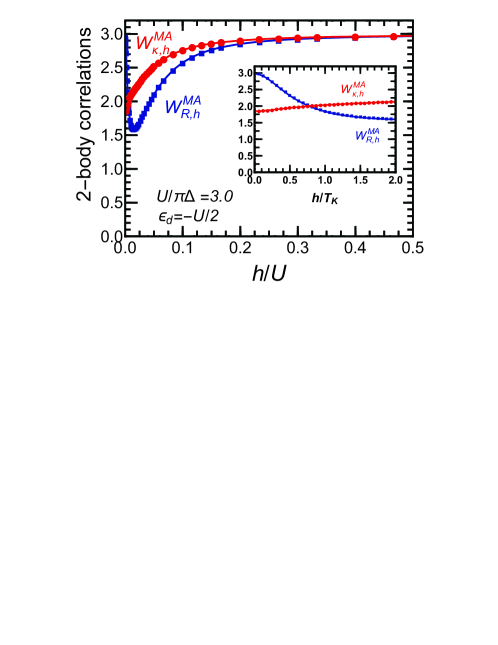
Figure 12: (Color online) Thermoelectric transport coefficients are plotted vs $h/U$ at half-filling $\epsilon_{d}=-U/2$ for $U/\pi\Delta=3.0$. Inset shows an enlarged view of the small $h$ region, for which the horizontal axis is scaled by $T_{K}=0.02\pi\Delta$ ($=0.0066U$) determined at $h=0$. Upper panel shows the contributions of two-body fluctuations $W_{R,h}^{\mathrm{MR}}$ and $W_{\kappa,h}^{\mathrm{MR}}$. Lower panel shows the coefficients $(48/\pi^{2})\,C_{R,h}^{\mathrm{MA}}=W_{R,h}^{\mathrm{MA}}+\Theta_{M}+\Theta_{X}$, and $(80/7\pi^{2})\,C_{\kappa,h}^{\mathrm{MA}}=W_{\kappa,h}^{\mathrm{MA}}+(13/21)\,\Theta_{M}+\Theta_{X}$ for the electric resistance $R_{\mathrm{MA}}$ and thermal conductivity $\kappa$. For the thermal conductivity, the two-body contribution becomes smallest $W_{\kappa,h}^{\mathrm{MA}}=13/7$ at $h=0$ and it increases with $h$. Magnetic-field dependence of the three-body contributions $\Theta_{M}$ and $\Theta_{X}$ are shown in Fig.  8.

VI.3 Thermoelectric effects at finite magnetic fields

We next examine thermoelectric effects at finite magnetic fields, specifically at half-filling $\epsilon_{d}=-U/2$. The thermopower vanishes $\mathcal{S}=0$ at half-filling also for $h\neq 0$ because the contributions of the two different spin states cancel out $\mathcal{L}_{1\uparrow}+\mathcal{L}_{1\downarrow}=0$. It can also be explained from the fact $\rho_{d\uparrow}^{\prime}+\rho_{d\downarrow}^{\prime}=0$. In this case, the density of states can be written in terms of the induced local moment, as $\rho_{d}=\cos^{2}\left(\frac{\pi m_{d}}{2}\right)/\pi\Delta$.

The magneto-resistance and thermal conductivity can be expressed in the following form at half-filling,

$$R_{\mathrm{MA}}={R_{\mathrm{MA}}^{0}}\left[\,\cos^{2}\left(\frac{\pi m_{d}}{2}\right)\,-\,C_{R,h}^{\mathrm{MA}}\left(\frac{\pi T}{T^{*}}\right)^{2}\,\right]+O(T^{4})\;,$$ (115)

$$\kappa=\frac{2\pi^{2}\eta_{0}}{3}\frac{T}{\cos^{2}\left(\frac{\pi m_{d}}{2}\right)}\,\left[\,1+\frac{C_{\kappa,h}^{\mathrm{MA}}}{\cos^{2}\left(\frac{\pi m_{d}}{2}\right)}\,\left(\frac{\pi T}{T^{*}}\right)^{2}\,\right]$$

$$\qquad+O(T^{5})\,.$$ (116)

Here, $T^{*}=1/(4\chi_{\uparrow\uparrow})$ is the field-dependent energy scale used in the previous section. The dimensionless coefficient for the electric resistance $R_{\mathrm{MA}}$ is given by

$$\!\!C_{R,h}^{\mathrm{MA}}\,\equiv\,\frac{\pi^{2}}{48}\left(\,W_{R,h}^{\mathrm{MA}}+\Theta_{M}+\Theta_{X}\right),$$ (117)

$$\!\!W_{R,h}^{\mathrm{MA}}\,=\,2-\cos\left(\pi m_{d}\right)+2\left(R_{W}-1\right)^{2}\cos\left(\pi m_{d}\right),\!\!$$ (118)

and that for the thermal conductivity $\kappa$ is

$$C_{\kappa,h}^{\mathrm{MA}}\equiv\frac{7\pi^{2}}{80}\left(W_{\kappa,h}^{\mathrm{MA}}+\frac{13}{21}\,\Theta_{M}+\Theta_{X}\right),$$ (119)

$$W_{\kappa,h}^{\mathrm{MA}}=2-\cos\left(\pi m_{d}\right)+\frac{6}{7}\left(R_{W}-1\right)^{2}\cos\left(\pi m_{d}\right).\!\!$$ (120)

The parameters $W_{R,h}^{\mathrm{MA}}$ and $W_{\kappa,h}^{\mathrm{MA}}$ represent the contribution of the two-body fluctuations, as determined by the induced local magnetization $m_{d}$ and the Wilson ratio $R_{W}$. The three-body contributions $\Theta_{M}$ and $\Theta_{X}$ have been defined in Eqs. (86a) and (86b), respectively, and the magnetic field dependence of these functions have also been described in Fig.  8. For large Coulomb interactions $U\gtrsim 2\pi\Delta$ at zero field $h=0$, the dimensionless coefficients take the values, $(48/\pi^{2})C_{R,h}^{\mathrm{MA}}=3$ and $(80/7\pi^{2})C_{\kappa,h}^{\mathrm{MA}}=13/7$, as $m_{d}=0$, $R_{W}\to 2$, $\Theta_{M}\to 0$, and $\Theta_{X}\to 0$. In the high-field limit $h\to\infty$, these two coefficients approach the noninteracting values, $(48/\pi^{2})C_{R,h}^{\mathrm{MA}}\to 1$ and $(80/7\pi^{2})C_{\kappa,h}^{\mathrm{MA}}\to 1$, as $m_{d}\to 1$, $R_{W}\to 1$, $\Theta_{M}\to 0$, and $\Theta_{X}\to-2$.

Figure 12 shows the $h$ dependence of these parameters for $U=3.0\pi\Delta$. The two-body contributions $W_{R,h}^{\mathrm{MA}}$ and $W_{\kappa,h}^{\mathrm{MA}}$ are positive and vary in a relatively small range from the high-field value $3.0$. For the thermal conductivity, it takes a minimum $W_{\kappa,h}^{\mathrm{MA}}=13/7$ at $h=0$ and increases with $h$. The electric resistance part has a minimum $W_{R,h}^{\mathrm{MA}}\simeq 1.6$ at a finite field $h\simeq 0.015U$. In contrast, the three-body contribution $\Theta_{M}$ has a much bigger dip as shown in Fig.  8. Therefore, the coefficients $C_{R,h}^{\mathrm{MA}}$ and $C_{\kappa,h}^{\mathrm{MA}}$ become negative in an intermediate region of the magnetic fields, typically $T_{K}\lesssim h\lesssim 0.1U$, while both of these two coefficients are positive outside of this region. The behavior in the high-filed limit is determined by the two-body contributions $W_{R,h}^{\mathrm{MA}}$ and $W_{\kappa,h}^{\mathrm{MA}}$, and the three-body contributions from $\Theta_{X}$.

VII Summary

In summary, we have studied low-energy properties of the steady-state Keldysh Green’s function in the situations where both the bias voltage and magnetic field are finite. The $(eV)^{2}$ real part of the self-energy has been deduced from the non-equilibrium Ward identities, using the previous result of the $\omega^{2}$ real part of the self-energy. Filippone et al. (2017); Oguri and Hewson (2018) We have also shown that the $(eV)^{2}$-correction and the $T^{2}$ correction of the self-energy are determined by a common correlation function, $\widehat{D}^{2}\Sigma_{\mathrm{eq},\sigma}^{--}(\omega)\equiv\Psi_{\sigma}^{--}(\omega)$. It indicates that these two corrections arise as a linear combination, $(\pi T)^{2}+(3/4)(eV)^{2}$, in the case where the bias voltages are applied such that $\alpha=0$. This output has previously been pointed out by FMvDM,Filippone et al. (2017) and our result provides an alternative proof.

We have applied the low-energy asymptotic form of the Green’s function given in Eqs. (53)–(54) to explore the non-linear magneto-conductance of quantum dots, and also the electric resistance and thermal conductivity of dilute magnetic alloys. The Fermi-liquid corrections in the general case are determined by two different types of contributions: the two-body-fluctuation contribution described by the susceptibilities $\chi_{\sigma\sigma^{\prime}}$ and the three-body-fluctuation contribution enters through the non-linear susceptibilities $\chi_{\sigma_{1}\sigma_{2}\sigma_{3}}^{[3]}$. Using the NRG, we have examined the $T^{2}$ and $(eV)^{2}$ corrections of the transport coefficients for some particle-hole asymmetric cases. At zero field, the two-body fluctuations dominate the corrections in the Kondo regime where $n_{d\uparrow}+n_{d\downarrow}\simeq 1$ and the Wilson ratio is almost saturated $R_{W}\simeq 2$. The contribution of the three-body fluctuations become significant far away from half-filling, especially in the valence-fluctuation regime and empty-orbital regime. Furthermore, we have also reexamined a controversial problem of the zero-bias peak of $dI/dV$ at finite magnetic fields. Hewson et al. (2005, 2006); Filippone et al. (2017) In this case, the three-body fluctuations give a contribution that is comparable to the two-body contribution even for small magnetic fields. The three-body contribution also plays essential role in a splitting of the zero-bias peak occurring at a magnetic field, $h\sim T_{K}$, of the order of the Kondo energy scale $T_{K}$. This observation based on the formula Eq. (82) is consistent with our previous result of the second-order renormalized perturbation theory.Hewson et al. (2005)

Furthermore, we have also studied the Fermi-liquid corrections for the magneto-resistance and thermal conductivity of dilute magnetic alloys away from half-filling. The NRG result shows that the contributions of the two-body fluctuations dominate in the Kondo regime, whereas in the valence-fluctuation regime far away from half-filling the contribution of three-body fluctuations become comparable to the two-body contribution. We have also provided the formulas for higher-order Fermi-liquid corrections for the Anderson impurity with $N$ flavor components in Appendix A. Further details of the multi-component case will be discussed elsewhere.

Appendix A The zero-frequency limit of $\Psi_{\sigma}^{--}(\omega)$ for an $N$-component Anderson impurity

It has been shown in Eq. (47) that $\widehat{D}^{2}\Sigma_{\mathrm{eq},\sigma}^{--}(\omega)\equiv\Psi_{\sigma}^{--}(\omega)$, which indicates that the common coefficient in the $(eV)^{2}$ and $T^{2}$ corrections to $\Sigma_{\mathrm{eq},\sigma}^{--}(\omega)$ is determined by the $\lim_{\omega\to 0}\Psi_{\sigma}^{--}(\omega)$. In this appendix, we calculate this value. In order to give a general derivation, which can also be applied to an Anderson impurity with a number of components, we extend the impurity part of the Hamiltonian such that

$$\mathcal{H}_{d}^{(N)}= \ \sum_{\sigma=1}^{N}\epsilon_{d\sigma}\,n_{d\sigma}+\frac{1}{2}\sum_{\sigma\neq\sigma^{\prime}}U_{\sigma\sigma^{\prime}}\,n_{d\sigma}n_{d,\sigma^{\prime}}\;.$$ (121)

The inter-electron interaction $U_{\sigma\sigma^{\prime}}$ generally depends on $\sigma$ and $\sigma^{\prime}$, with the requirements $U_{\sigma^{\prime}\sigma}=U_{\sigma\sigma^{\prime}}$ for $\sigma^{\prime}\neq\sigma$. For $N=2$, it describes the single-orbital Anderson model for spin $1/2$ fermions which we have considered so far. The remaining part of the Hamiltonian takes the same form as Eqs. (2) and (3) but the index runs over $\sigma=1,2,\ldots,N$. Namely, the free conduction band $\mathcal{H}_{c}$ also consists of $N$ flavor components, and $\mathcal{H}_{\mathrm{T}}$ describes the tunnelings that preserve the index $\sigma$. One of the features of interest in the multi-component impurity is that for $N>2$ the three-body correlations $\chi_{\sigma_{1}\sigma_{2}\sigma_{3}}^{[3]}$ among three different components $\sigma_{1}\neq\sigma_{2}\neq\sigma_{3}\neq\sigma_{1}$ also contribute to the low-energy properties.

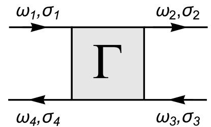
Figure 13: Vertex function $\Gamma_{\sigma_{1}\sigma_{2};\sigma_{3}\sigma_{4}}(\omega_{1},\omega_{2};\omega_{3},\omega_{4})$.

For general $N$, the function $\Psi_{\sigma}^{--}$ is defined by

$$\Psi_{\sigma}^{--}(\omega)\equiv\lim_{\omega^{\prime}\to 0}\frac{\partial}{\partial\omega^{\prime}}\sum_{\sigma^{\prime}=1}^{N}\Gamma_{\sigma\sigma^{\prime};\sigma^{\prime}\sigma}(\omega,\omega^{\prime};\omega^{\prime},\omega)\rho_{d\sigma^{\prime}}(\omega^{\prime}),$$ (122)

in terms of the vertex function illustrated in Fig. 13. We show in the following that the zero-frequency limit is given by

$$\lim_{\omega\to 0}\Psi_{\sigma}^{--}(\omega)=\frac{1}{\rho_{d\sigma}}\!\sum_{\sigma^{\prime}(\neq\sigma)}\frac{\partial\chi_{\sigma\sigma^{\prime}}}{\partial\epsilon_{d\sigma^{\prime}}}-i\frac{3\pi}{\rho_{d\sigma}}\!\sum_{\sigma^{\prime}(\neq\sigma)}\!\chi_{\sigma\sigma^{\prime}}^{2}\,\mbox{sgn}(\omega)$$ (123)

The vertex function $\Gamma_{\sigma\sigma^{\prime};\sigma^{\prime}\sigma}(\omega,\omega^{\prime};\omega^{\prime},\omega)$ has lines of singularities along $\omega-\omega^{\prime}=0$ and $\omega+\omega^{\prime}=0$.Yoshimori (1976); Eliashberg (1962a, b) For small $\omega$ and $\omega^{\prime}$, these singularities emerge through the three diagrams shown in Fig. 14, and the imaginary part of $\Psi_{\sigma}^{--}(\omega)$ can be calculated asOguri (2001)

$$\sum_{\sigma^{\prime}}\rho_{d\sigma^{\prime}}\,\mathrm{Im}\,\frac{\partial}{\partial\omega^{\prime}}\Gamma_{\sigma\sigma^{\prime};\sigma^{\prime}\sigma}(\omega,\omega^{\prime};\omega^{\prime},\omega)$$

$$=-\,\sum_{\sigma^{\prime}(\neq\sigma)}\left|\Gamma_{\sigma\sigma^{\prime};\sigma^{\prime}\sigma}(0,0;0,0)\right|^{2}$$

$$\ \times\mathrm{Im}\Biggl{[}\ \int\frac{d\omega^{\prime\prime}}{2\pi i}\,G_{\mathrm{eq},\sigma^{\prime}}^{--}(\omega^{\prime\prime})\,\frac{\partial}{\partial\omega^{\prime}}\,G_{\mathrm{eq},\sigma^{\prime}}^{--}(\omega-\omega^{\prime}+\omega^{\prime\prime})\,\rho_{d\sigma}$$

$$\ +\int\frac{d\omega^{\prime\prime}}{2\pi i}\,G_{\mathrm{eq},\sigma^{\prime}}^{--}(\omega^{\prime\prime})\,\frac{\partial}{\partial\omega^{\prime}}\,G_{\mathrm{eq},\sigma}^{--}(\omega-\omega^{\prime}+\omega^{\prime\prime})\,\rho_{d\sigma^{\prime}}$$

$$\ +\int\frac{d\omega^{\prime\prime}}{2\pi i}\,G_{\mathrm{eq},\sigma^{\prime}}^{--}(\omega^{\prime\prime})\,\frac{\partial}{\partial\omega^{\prime}}\,G_{\mathrm{eq},\sigma}^{--}(\omega+\omega^{\prime}-\omega^{\prime\prime})\,\rho_{d\sigma^{\prime}}\,\Biggr{]}+\cdots$$

$$=\,-\,\pi\sum_{\sigma^{\prime}(\neq\sigma)}\left|\Gamma_{\sigma\sigma^{\prime};\sigma^{\prime}\sigma}(0,0;0,0)\right|^{2}$$

$$\qquad\qquad\times\rho_{d\sigma}\rho_{d\sigma^{\prime}}^{2}\Bigl{[}\,2\,\mbox{sgn}(\omega-\omega^{\prime})+\,\mbox{sgn}(\omega+\omega^{\prime})\,\Bigr{]}+\cdots$$

$$=-\pi\sum_{\sigma^{\prime}(\neq\sigma)}\frac{\chi_{\sigma\sigma^{\prime}}^{2}}{\rho_{d\sigma}}\Bigl{[}\,2\,\mbox{sgn}(\omega-\omega^{\prime})\,+\mbox{sgn}(\omega+\omega^{\prime})\,\Bigr{]}+\cdots\;.$$ (124)

In the second line, the three integrals correspond to contributions of each diagram shown in Fig.  14. The left and middle diagrams yield the non-analytic $2\,\mbox{sgn}(\omega-\omega^{\prime})$ contribution due to the particle-hole pair excitation, and the right diagram yields the $\mbox{sgn}(\omega+\omega^{\prime})$ contribution due to the particle-particle pair excitation. Taking first the limit $\omega^{\prime}\to 0$ keeping the external frequency $\omega$ finite, we obtain the imaginary part of Eq. (47),

$$\lim_{\omega\to 0}\,\mathrm{Im}\,\Psi_{\sigma}^{--}(\omega)=-3\pi\sum_{\sigma^{\prime}(\neq\sigma)}\frac{\chi_{\sigma\sigma^{\prime}}^{2}}{\rho_{d\sigma}}\,\mbox{sgn}(\omega)\,.$$ (125)

   

Figure 14: Feynman diagrams which provide the imaginary part to the vertex function $\Gamma_{\sigma\sigma^{\prime};\sigma^{\prime}\sigma}(\omega,\omega^{\prime};\omega^{\prime},\omega)$ for small $\omega$ and $\omega^{\prime}$. The shaded square represents the zero-frequency vertex part $\Gamma_{\sigma,\sigma^{\prime\prime};\sigma^{\prime\prime}\sigma}(0,0;0,0)$, which for $\sigma^{\prime\prime}=\sigma$ identically vanishes $\Gamma_{\sigma\sigma;\sigma\sigma}(0,0;0,0)=0$. The singular $\mathrm{sgn}\,(\omega-\omega^{\prime})$ term arises from the intermediate particle-hole excitation with $\sigma^{\prime}=\sigma$ shown in the left panel, and also from the particle-hole pair with $\sigma^{\prime}\neq\sigma$ in the middle panel. Another singular term $\mathrm{sgn}\,(\omega+\omega^{\prime})$ arises from the particle-particle pair excitation with $\sigma^{\prime}\neq\sigma$ in the right panel.

The real part of $\Psi_{\sigma}^{--}(\omega)$ does not have the non-analytic $\mathrm{sgn}(\omega)$ dependence, and it can be deduced from Eq. (47) by taking first the $\omega\to 0$ limit,

$$\mathrm{Re}\,\Psi_{\sigma}^{--}(0)\,= \ \sum_{\sigma^{\prime}}\rho_{d\sigma^{\prime}}\left.\frac{\partial}{\partial\omega^{\prime}}\mathrm{Re}\,\Gamma_{\sigma\sigma^{\prime};\sigma^{\prime}\sigma}(0,\omega^{\prime};\omega^{\prime},0)\,\right|_{\omega^{\prime}=0}$$

$$\ +\sum_{\sigma^{\prime}(\neq\sigma)}\Gamma_{\sigma\sigma^{\prime};\sigma^{\prime}\sigma}(0,0;0,0)\,\rho_{d\sigma^{\prime}}^{\prime}.$$ (126)

The second term of Eq. (126) can be expressed in the form

$$\sum_{\sigma^{\prime}(\neq\sigma)}\Gamma_{\sigma\sigma^{\prime};\sigma^{\prime}\sigma}(0,0;0,0)\,\rho_{d\sigma^{\prime}}^{\prime}=-\sum_{\sigma^{\prime}(\neq\sigma)}\frac{\chi_{\sigma\sigma^{\prime}}}{\rho_{d\sigma}\rho_{d\sigma^{\prime}}}\rho_{d\sigma^{\prime}}^{\prime}.$$ (127)

The first term of Eq. (126) can be calculated as

$$\!\!\!\!\!\!\!\!\!\!\sum_{\sigma^{\prime}}\rho_{d\sigma^{\prime}}\left.\frac{\partial}{\partial\omega^{\prime}}\,\mathrm{Re}\,\Gamma_{\sigma\sigma^{\prime};\sigma^{\prime}\sigma}(0,\omega^{\prime};\omega^{\prime},0)\,\,\right|_{\omega^{\prime}=0}$$

$$=\,\sum_{\sigma^{\prime}}\rho_{d\sigma^{\prime}}\left.\frac{\partial}{\partial\omega^{\prime}}\,\mathrm{Re}\,\Gamma_{\sigma^{\prime}\sigma;\sigma\sigma^{\prime}}(\omega^{\prime},0;0,\omega^{\prime})\,\,\right|_{\omega^{\prime}=0}$$

$$=\,\sum_{\sigma^{\prime}(\neq\sigma)}\rho_{d\sigma^{\prime}}\left.\frac{\partial}{\partial\omega^{\prime}}\,\mathrm{Re}\,\Gamma_{\sigma^{\prime}\sigma;\sigma\sigma^{\prime}}(\omega^{\prime},0;0,\omega^{\prime})\,\right|_{\omega^{\prime}=0}$$

$$=\,-\sum_{\sigma^{\prime}(\neq\sigma)}\rho_{d\sigma^{\prime}}\left.\frac{\partial}{\partial\omega}\,\frac{1}{\rho_{d\sigma}}\frac{\partial\,\mathrm{Re}\,\Sigma^{--}_{\text{eq},\sigma^{\prime}}(\omega)}{\partial\epsilon_{d\sigma}}\,\right|_{\omega=0}$$

$$=\,\sum_{\sigma^{\prime}(\neq\sigma)}\frac{\rho_{d\sigma^{\prime}}}{\rho_{d\sigma}}\frac{\partial}{\partial\epsilon_{d\sigma}}\!\left.\left(1-\frac{\partial\,\Sigma^{--}_{\text{eq},\sigma^{\prime}}(\omega)}{\partial\omega}\right)\right|_{\omega=0}$$

$$=\,\sum_{\sigma^{\prime}(\neq\sigma)}\frac{\rho_{d\sigma^{\prime}}}{\rho_{d\sigma}}\frac{\partial\widetilde{\chi}_{\sigma^{\prime}\sigma^{\prime}}}{\partial\epsilon_{d\sigma}}=\sum_{\sigma^{\prime}(\neq\sigma)}\frac{\rho_{d\sigma^{\prime}}}{\rho_{d\sigma}}\frac{\partial\widetilde{\chi}_{\sigma^{\prime}\sigma}}{\partial\epsilon_{d\sigma^{\prime}}}$$

$$= \frac{1}{\rho_{d\sigma}}\sum_{\sigma^{\prime}(\neq\sigma)}\left(\frac{\partial\chi_{\sigma\sigma^{\prime}}}{\partial\epsilon_{d\sigma^{\prime}}}-\frac{\chi_{\sigma\sigma^{\prime}}}{\rho_{d\sigma^{\prime}}}\,\frac{\partial\rho_{d\sigma^{\prime}}}{\partial\epsilon_{d\sigma^{\prime}}}\right).$$ (128)

Note that $\Gamma_{\sigma\sigma^{\prime};\sigma^{\prime}\sigma}(0,\omega^{\prime};\omega^{\prime},0)=\Gamma_{\sigma^{\prime}\sigma;\sigma\sigma^{\prime}}(\omega^{\prime},0;0,\omega^{\prime})$, the symmetric property of the vertex function has been used to obtain the second line. To obtain the third line, we have used the property that the vertex function for the parallel spins $\Gamma_{\sigma\sigma;\sigma\sigma}(\omega,0;0,\omega)$ has no $\omega$-linear real part, which has been shown in paper II.Oguri and Hewson (2018) Therefore we obtain the following result from Eqs. (126)–(127), using Eq. (21) for the density of states:

$$\mathrm{Re}\,\Psi_{\sigma}^{--}(0)\,=\,\frac{1}{\rho_{d\sigma}}\sum_{\sigma^{\prime}(\neq\sigma)}\frac{\partial\chi_{\sigma\sigma^{\prime}}}{\partial\epsilon_{d\sigma^{\prime}}}\;.$$ (129)

The $(eV)^{2}$ and $T^{2}$ contributions of $\mathrm{Re}\,\Sigma_{\mathrm{eq},\sigma}^{--}(0)$ arise from the intermediate single-particle excitation which carries the different flavor indexes $\sigma^{\prime}$ from the external one $\sigma$.

From these results, the vertex function for $\Gamma_{\sigma\sigma^{\prime};\sigma^{\prime}\sigma}(\omega,\omega^{\prime};\omega^{\prime},\omega)$ can also be deduced. For $\sigma^{\prime}=\sigma$, it takes the form

$$\!\!\!\!\!\Gamma_{\sigma\sigma;\sigma\sigma}(\omega,\omega^{\prime};\omega^{\prime},\omega)\rho_{d\sigma}^{2}=i\pi\sum_{\sigma^{\prime}(\neq\sigma)}\chi_{\sigma\sigma^{\prime}}^{2}\bigl{|}\omega-\omega^{\prime}\bigr{|}+\cdots\!,\!\!$$ (130)

and it for $\sigma^{\prime}\neq\sigma$ is

$$\Gamma_{\sigma\sigma^{\prime};\sigma^{\prime}\sigma}(\omega,\omega^{\prime};\omega^{\prime},\omega)\,\rho_{d\sigma}\rho_{d\sigma^{\prime}}\ =$$

$$\qquad-\chi_{\sigma\sigma^{\prime}}+\rho_{d\sigma}\frac{\partial\widetilde{\chi}_{\sigma\sigma^{\prime}}}{\partial\epsilon_{d\sigma}}\,\omega+\rho_{d\sigma^{\prime}}\frac{\partial\widetilde{\chi}_{\sigma^{\prime}\sigma}}{\partial\epsilon_{d\sigma^{\prime}}}\,\omega^{\prime}$$

$$\qquad+i\pi\,\chi_{\sigma\sigma^{\prime}}^{2}\Bigl{(}\,\bigl{|}\omega-\omega^{\prime}\bigr{|}-\,\bigl{|}\omega+\omega^{\prime}\bigr{|}\Bigr{)}+\cdots.$$ (131)

These results and the $\omega^{2}$ contribution of the self-energy are related each other via the Ward identity, given in Eq. (23).

Appendix B Coefficients $\alpha_{2\sigma}$ & $\phi_{2\sigma}$ of FMvDM

In this appendix, we summarize the relation between the parameters used in the description of FMvDM and the derivative of the susceptibilities. The coefficients $\alpha_{1\sigma}$ and $\phi_{1}$ are the parameters which were introduced by Nozières for his phenomenological description,

$$\frac{\alpha_{1\sigma}}{\pi}\,=\,\chi_{\sigma\sigma}\,,\qquad\ \ \frac{\phi_{1}}{\pi}\,=\,-\chi_{\uparrow\downarrow}\,.$$ (132)

Note that $\chi_{\uparrow\downarrow}=\chi_{\downarrow\uparrow}$ and it is an even function of $h$ because of $\Omega$ is an even function of $h$, as mentioned.

The coefficients $\alpha_{2\sigma}$ and $\phi_{2\sigma}$ defined in Eqs. (13a)–(13d) of the FMvDM’s paperFilippone et al. (2017) can also be written in terms of the susceptibilities. Substituting the charge and spin susceptibilities, $\chi_{c}\equiv\chi_{\uparrow\uparrow}+\chi_{\downarrow\downarrow}+\chi_{\uparrow\downarrow}+\chi_{\downarrow\uparrow}$ and $\chi_{s}\equiv\displaystyle\frac{1}{4}\left(\chi_{\uparrow\uparrow}+\chi_{\downarrow\downarrow}-\chi_{\uparrow\downarrow}-\chi_{\downarrow\uparrow}\right)$, into the definitions and rescaling the magnetic field as $B=2h$,

$$\frac{\alpha_{2\uparrow}+\alpha_{2\downarrow}}{2\pi}\,= \ -\frac{3}{4}\frac{\partial\chi_{s}}{\partial\epsilon_{d}}-\frac{1}{16}\frac{\partial\chi_{c}}{\partial\epsilon_{d}}$$

$$\!\!\!\!\!\!\!\!\!\!\!\!\!\!\!\!\!\!\!\!\!\!\!\!\!\!\!\!\!\!\!\!=\frac{1}{8}\left(\frac{\partial}{\partial\epsilon_{d\uparrow}}+\frac{\partial}{\partial\epsilon_{d\downarrow}}\right)\Bigl{[}-2\left(\chi_{\uparrow\uparrow}+\chi_{\downarrow\downarrow}\right)+\left(\chi_{\uparrow\downarrow}+\chi_{\downarrow\uparrow}\right)\Bigr{]},$$ (133)

$$\frac{\alpha_{2\uparrow}-\alpha_{2\downarrow}}{2\pi}\,= \ \frac{1}{2}\frac{\partial\chi_{s}}{\partial B}+\frac{3}{8}\frac{\partial\chi_{c}}{\partial B}$$

$$\!\!\!\!\!\!\!\!\!\!\!\!\!\!\!\!\!\!\!\!\!\!\!\!\!\!\!\!\!\!\!\!=\frac{1}{8}\left(-\frac{\partial}{\partial\epsilon_{d\uparrow}}+\frac{\partial}{\partial\epsilon_{d\downarrow}}\right)\Bigl{[}2\left(\chi_{\uparrow\uparrow}+\chi_{\downarrow\downarrow}\right)+\left(\chi_{\uparrow\downarrow}+\chi_{\downarrow\uparrow}\right)\Bigr{]},$$ (134)

$$\frac{\phi_{2\uparrow}+\phi_{2\downarrow}}{2\pi}\,= \ -\frac{\partial\chi_{s}}{\partial\epsilon_{d}}+\frac{1}{4}\frac{\partial\chi_{c}}{\partial\epsilon_{d}}$$

$$\,= \ \frac{1}{2}\left(\frac{\partial}{\partial\epsilon_{d\uparrow}}+\frac{\partial}{\partial\epsilon_{d\downarrow}}\right)\left(\chi_{\uparrow\downarrow}+\chi_{\downarrow\uparrow}\right)\;,$$ (135)

$$\frac{\phi_{2\uparrow}-\phi_{2\downarrow}}{2\pi}\,= \ 2\frac{\partial\chi_{s}}{\partial B}-\frac{1}{2}\frac{\partial\chi_{c}}{\partial B}$$

$$\,= \ \frac{-1}{2}\left(-\frac{\partial}{\partial\epsilon_{d\uparrow}}+\frac{\partial}{\partial\epsilon_{d\downarrow}}\right)\left(\chi_{\uparrow\downarrow}+\chi_{\downarrow\uparrow}\right).$$ (136)

Thus, the coefficients $\alpha_{2\sigma}$ and $\phi_{2\sigma}$ can be expressed in the form

$$\frac{\alpha_{2\sigma}}{\pi}\,= \ -\frac{1}{2}\,\frac{\partial\chi_{\sigma\sigma}}{\partial\epsilon_{d\sigma}}\;,\qquad\ \frac{\phi_{2\sigma}}{\pi}\,=\,2\,\frac{\partial\chi_{\uparrow\downarrow}}{\partial\epsilon_{d\sigma}}\;.$$ (137)

Using these relations, the coefficient for the $\omega^{2}$ real part of the self-energy, provided in Eqs. (B2a) and (B8b) of FMvDM’s paper,Filippone et al. (2017) can be confirmed to agree with Eq. (28) of ours:

$$\!\!\!\frac{\widetilde{R}_{\sigma,\omega}}{z_{\sigma}}\,=\,\frac{\alpha_{2\sigma}}{\pi\rho_{d\sigma}}-\frac{\pi\rho_{d\sigma}}{z_{\sigma}^{2}}\cot\delta_{\sigma}$$

$$\ \ =-\frac{1}{2\rho_{d\sigma}}\!\left(\frac{\partial\chi_{\sigma\sigma}}{\partial\epsilon_{d\sigma}}+2\pi\cot\delta_{\sigma}\chi_{\sigma\sigma}^{2}\right)=-\frac{1}{2}\frac{\partial\widetilde{\chi}_{\sigma\sigma}}{\partial\epsilon_{d\sigma}}.$$ (138)

We have also used Eq. (20) to obtain the last line.

Appendix C Comparison with $\mathrm{Re}\,\Sigma^{r}(\omega,eV)$ described in Ref. Oguri, 2001

The explicit low-energy expression of the real part of the self-energy given in Eq. (54) reproduces at zero magnetic field $h=0$ the previous result, reported in Eq. (19) of Ref. Oguri, 2001. It was written in such a way that the coefficient for the $\omega^{2}$ real part, $b$, as an additional parameter that had not been related to the other renormalized parameters

$$b\,\equiv\,\left.\mathrm{Re}\,\frac{\partial^{2}\Sigma_{\mathrm{eq}}^{r}(\omega)}{\partial\omega^{2}}\right|_{\omega=0}\;.$$ (139)

Recent development clarifies that this coefficient can be written in terms of the derivative of the static susceptibilities $b={\partial\widetilde{\chi}_{\uparrow\uparrow}}/{\partial\epsilon_{d\uparrow}}$, as mentioned for Eq. (28). With this recent knowledge, we can explicitly confirm that the previous result is completely identical to Eq. (55).

The coefficients for $\omega eV$ and $\alpha^{2}(eV)^{2}$ terms in Eq. (19) of Ref. Oguri, 2001 can be written, respectively, as

$$-\left(b-\frac{\partial\widetilde{\chi}_{\uparrow\uparrow}}{\partial\epsilon_{d}}\right)= -\frac{\partial\widetilde{\chi}_{\uparrow\uparrow}}{\partial\epsilon_{d\uparrow}}+\frac{\partial\widetilde{\chi}_{\uparrow\uparrow}}{\partial\epsilon_{d}}=\frac{\partial\widetilde{\chi}_{\uparrow\uparrow}}{\partial\epsilon_{d\downarrow}}$$

$$= \ \frac{\partial\widetilde{\chi}_{\uparrow\downarrow}}{\partial\epsilon_{d\uparrow}},$$ (140)

$$b-\frac{\partial\widetilde{\chi}_{s}}{\partial\epsilon_{d}}= \frac{\partial\widetilde{\chi}_{\uparrow\uparrow}}{\partial\epsilon_{d\uparrow}}-\frac{\partial}{\partial\epsilon_{d}}\left(\widetilde{\chi}_{\uparrow\uparrow}-\widetilde{\chi}_{\uparrow\downarrow}\right)$$

$$= \ -\frac{\partial\widetilde{\chi}_{\uparrow\downarrow}}{\partial\epsilon_{d\uparrow}}+\frac{\partial\widetilde{\chi}_{\uparrow\downarrow}}{\partial\epsilon_{d}}=\frac{\partial\widetilde{\chi}_{\uparrow\downarrow}}{\partial\epsilon_{d\downarrow}}.$$ (141)

These coefficients agree with the corresponding results given in Eq. (54) for $\sigma=\uparrow$ and $h=0$. Furthermore, the coefficient for the $(eV)^{2}$ term that emerges through the $\widehat{D}^{2}$ operator can be written in the form,

$$-\lim_{h\to 0}\left(b-\frac{\partial\widetilde{\chi}_{\uparrow\uparrow}}{\partial\epsilon_{d}}+\frac{\rho_{d}^{\prime}}{\rho_{d}}\,\widetilde{\chi}_{\uparrow\downarrow}\right)\,=\,\lim_{h\to 0}\left(\frac{\partial\widetilde{\chi}_{\uparrow\downarrow}}{\partial\epsilon_{d\uparrow}}-\frac{\chi_{\uparrow\downarrow}}{\rho_{d}^{2}}\,\rho_{d}^{\prime}\right)$$

$$\quad=\,\lim_{h\to 0}\left[\frac{\partial}{\partial\epsilon_{d\uparrow}}\left(\frac{\chi_{\uparrow\downarrow}}{\rho_{d\uparrow}}\right)+\frac{\chi_{\uparrow\downarrow}}{\rho_{d\uparrow}^{2}}\,\frac{\partial\rho_{d\uparrow}}{\partial\epsilon_{d\uparrow}}\right]=\,\lim_{h\to 0}\frac{1}{\rho_{d\uparrow}}\frac{\partial\chi_{\uparrow\downarrow}}{\partial\epsilon_{d\uparrow}}$$

$$\quad=\lim_{h\to 0}\frac{1}{\rho_{d\uparrow}}\frac{\partial\chi_{\uparrow\downarrow}}{\partial\epsilon_{d\downarrow}}\;.$$ (142)

This agrees with the general result, given in Eq. (129).

Appendix D Erratum for the original version
Phys. Rev. B 97, 035435 (2018)

After we published the original version of this paper, we found some errors which should be corrected. We summarized the changes in this appendix, which have already been corrected in this version. All the errors occurred only in the applications to some special cases. The general Fermi-liquid relations for the self-energy, vertex functions, and transport coefficients, described in the original paper, are not affected by these revisions.

The first point is that, in figures 4 and 5 of our paper, the results for the three-body correlation function for the up- and down-spins $\Theta_{\uparrow\downarrow}$ at zero magnetic field were plotted with the wrong sign. These figures have been corrected in the version 3.

The other errors arose for the magneto-transport coefficients, which have been studied at half-filling $\epsilon_{d}=-U/2$ in Sec. V C, Sec. VI C, and Appendix C. The central point is that there is an additional three-body term at finite magnetic fields, which was not taken into account properly in these sections. It is simply an error occurring in the application as the general Fermi-liquid relations that we described naturally yield the additional term. This term, which we write $\Theta_{X}$, gives finite contributions together with the other three-body term $\Theta_{M}$ that has been described in detail in the original paper: Eq. (5.28) has been replaced by the following form,  adding the second line for $\Theta_{X}$,

$$\Theta_{M}\,\equiv \ -\,\frac{\sin(\pi m_{d})}{2\pi}\frac{1}{\chi_{\uparrow\uparrow}^{2}}\,\frac{\partial\chi_{\uparrow\downarrow}}{\partial h}\,,\qquad\qquad\qquad\quad\ \,(5.28a)$$

$$\Theta_{X}\,\equiv \ -\,\frac{\sin(\pi m_{d})}{2\pi}\frac{1}{\chi_{\uparrow\uparrow}^{2}}\frac{\partial}{\partial\epsilon_{d}}\left(\frac{\chi_{\uparrow\uparrow}-\chi_{\downarrow\downarrow}}{2}\right)\;.\qquad(5.28b)$$

The additional contribution of $\Theta_{X}$ also appears in Eqs. (5.23), (5.24), (5.25), (6.27), (6.29), (C.5), and (C.6): these equations have been corrected in this version 4.

Correspondingly, the NRG results for the transport coefficients, presented in the lower panel of Fig. 8 and the upper panel of Figs. 9 and 12, have also been replaced by the new ones. As shown in new Fig. 8, $\Theta_{X}$ becomes zero at $h=0$, and is very small for low fields $h\lesssim T_{K}$. It becomes comparable to $\Theta_{M}$ at $h\gtrsim 0.1U$, and in the high-field limit $h\to\infty$ it approaches $\Theta_{X}\to-2$ where the interaction $U$ becomes less important. Therefore, major changes appear only at high fields: the coefficients approach $(48/\pi^{2})C_{T}^{h}\to-3$ and $(64/\pi^{2})C_{V}^{h}\to-3$ in Fig. 9, and $(48/\pi^{2})C_{R,h}^{\mathrm{MA}}\to 1$ and $(80/7\pi^{2})C_{\kappa,h}^{\mathrm{MA}}\to 1$ in Fig. 12. For low-field behavior of these coefficients, however, $\Theta_{X}$ does not cause visible changes. We have confirmed that the contribution of $\Theta_{X}$ becomes smaller than the symbol size for the lines shown in the lower panel of Fig. 9, in which the rescaled values of the conductance coefficients, $\overline{C}_{T}^{h}$ and $\overline{C}_{V}^{h}$, are plotted for $0<h<0.5T_{K}$.

References

- Nozières (1974) P. Nozières, J. Low Temp. Phys. 17, 31 (1974).
- Yamada (1975a) K. Yamada, Prog. Theor. Phys. 53, 970 (1975a).
- Yamada (1975b) K. Yamada, Prog. Theor. Phys. 54, 316 (1975b).
- Shiba (1975) H. Shiba, Prog. Theor. Phys. 54, 967 (1975).
- Yoshimori (1976) A. Yoshimori, Prog. Theor. Phys. 55, 67 (1976).
- Wilson (1975) K. G. Wilson, Rev. Mod. Phys. 47, 773 (1975).
- Krishna-murthy et al. (1980a) H. R. Krishna-murthy, J. W. Wilkins, and K. G. Wilson, Phys. Rev. B 21, 1003 (1980a).
- Krishna-murthy et al. (1980b) H. R. Krishna-murthy, J. W. Wilkins, and K. G. Wilson, Phys. Rev. B 21, 1044 (1980b).
- Mora et al. (2015) C. Mora, C. P. Moca, J. von Delft, and G. Zaránd, Phys. Rev. B 92, 075120 (2015).
- Filippone et al. (2017) M. Filippone, C. P. Moca, J. von Delft, and C. Mora, Phys. Rev. B 95, 165404 (2017).
- Hershfield et al. (1992) S. Hershfield, J. H. Davies, and J. W. Wilkins, Phys. Rev. B 46, 7046 (1992).
- Oguri (2001) A. Oguri, Phys. Rev. B 64, 153305 (2001).
- Aligia (2012) A. A. Aligia, J. Phys.: Condens. Matter 24, 015306 (2012).
- Muñoz et al. (2013) E. Muñoz, C. J. Bolech, and S. Kirchner, Phys. Rev. Lett. 110, 016601 (2013).
- (15) A. Oguri and A. C. Hewson, arXiv:1709.06385 .
- Oguri and Hewson (2018) A. Oguri and A. C. Hewson, Phys. Rev. B 97, 045406 (2018).
- Glazman and Raikh (1988) L. I. Glazman and M. E. Raikh, JETP Lett. 47, 452 (1988).
- Ng and Lee (1988) T. K. Ng and P. A. Lee, Phys. Rev. Lett. 61, 1768 (1988).
- Wingreen and Meir (1994) N. S. Wingreen and Y. Meir, Phys. Rev. B 49, 11040 (1994).
- Meir and Wingreen (1992) Y. Meir and N. S. Wingreen, Phys. Rev. Lett. 68, 2512 (1992).
- Costi et al. (1994) T. A. Costi, A. C. Hewson, and V. Zlatić, J. Phys.: Condens. Matter 6, 2519 (1994).
- Oguri and Maekawa (1990) A. Oguri and S. Maekawa, Phys. Rev. B 41, 6977 (1990).
- Hewson (2001) A. C. Hewson, J. Phys.: Condens. Matter 13, 10011 (2001).
- Abrikosov et al. (1965) A. A. Abrikosov, I. Dzyaloshinskii, and L. P. Gorkov, Methods of Quantum Field Theory in Statistical Physics (Pergamon, London, 1965).
- Keldysh (1965) L. V. Keldysh, Sov. Phys. JETP 20, 1018 (1965).
- Caroli et al. (1971) C. Caroli, R. Combescot, and P. Nozières, Phys. C: Solid State Phys 4, 916 (1971).
- Eliashberg (1962a) G. M. Eliashberg, Sov. Phys. JETP 14, 886 (1962a).
- Eliashberg (1962b) G. M. Eliashberg, Sov. Phys. JETP 15, 1151 (1962b).
- Hewson et al. (2004) A. C. Hewson, A. Oguri, and D. Meyer, Eur. Phys. J. B 40, 177 (2004).
- Amit and Martín-Mayor (2005) D. Amit and V. Martín-Mayor, Field Theory, the Renormalization Group, and Critical Phenomena (World Scientific, Singapore, 2005).
- Hewson et al. (2006) A. C. Hewson, J. Bauer, and W. Koller, Phys. Rev. B 73, 045117 (2006).
- Hewson et al. (2005) A. C. Hewson, J. Bauer, and A. Oguri, J. Phys.: Condens. Matter 17, 5413 (2005).
- Guttman et al. (1995) G. D. Guttman, E. Ben-Jacob, and D. J. Bergman, Phys. Rev. B 51, 17758 (1995).
- Note (1) Thermoelectric response of quantum dots is described by the coefficients: .