Dissecting the hadronic contributions to $(g-2)_{\upmu}$ by Schwinger’s sum rule

Abstract

The theoretical uncertainty of $(g-2)_{\upmu}$ is currently dominated by hadronic contributions. In order to express those in terms of directly measurable quantities, we consider a sum rule relating $g-2$ to an integral of a photo-absorption cross section. The sum rule, attributed to Schwinger, can be viewed as a combination of two older sum rules: Gerasimov-Drell-Hearn and Burkhardt-Cottingham. The Schwinger sum rule has an important feature, distinguishing it from the other two: the relation between the anomalous magnetic moment and the integral of a photo-absorption cross section is linear, rather than quadratic. The linear property makes it suitable for a straightforward assessment of the hadronic contributions to $(g-2)_{\upmu}$. From the sum rule we rederive the Schwinger $\alpha/2\pi$ correction, as well as the formula for the hadronic vacuum-polarization contribution. As an example of the light-by-light contribution we consider the single-meson exchange.

I Introduction

The anomalous magnetic moment (AMM) of the muon, $\varkappa_{\upmu}\equiv\nicefrac{{1}}{{2}}(g-2)_{\upmu}$, serves as a stringent precision tests of the Standard Model (SM). And at present it does not work out for the SM — the experimental value is about $3\sigma$ away from the SM prediction Blum:2013xva ; Benayoun:2014tra . While the uncertainties of the SM and the experimental value are comparable, the new Fermilab experiment Logashenko:2015xab ; Venanzoni:2014ixa will, in a few years, reduce the experimental error-bar by nearly a factor of four. The prospects for reducing the SM (theory) uncertainty are, on the other hand, more obscure. The SM error-bar is dominated by the hadronic contributions, which are very difficult to compute in the SM due to the non-perturbative nature of Quantum Chromodynamics (QCD). In the present SM value these contributions are determined empirically, using general relations to other experimental observables in combination with mesonic model calculations, rather than from QCD directly. It is the necessity of resorting to models — particularly in evaluation of the so-called hadronic light-by-light (HLbL) contributions [c.f. Fig. 1(b)] — which makes it difficult to reduce the uncertainty of the current SM value.

In the future, lattice QCD will deliver a sufficiently precise ab initio calculation of the HLbL contribution; for recent progress in this direction see Refs. Blum:2014oka ; Blum:2015gfa ; Green:2015sra ; Green:2015mva . Until then, the best hope for improvement is to replace the model evaluations with model-independent, “data-driven” approaches based on dispersion theory. The data-driven approach is fairly well-founded and routinely used for the hadronic vacuum-polarization (HVP) contribution [Fig. 1(a)], since it can exactly be written as a dispersion integral of the decay rate of a virtual timelike photon into hadrons, which to a good approximation is expressed in terms of the observed ratio $\mu^{+}\mu^{-}/e^{+}e^{-}\to\mathrm{hadrons}$, see e.g., Refs. Jegerlehner:2017gek ; Davier:2016iru . The HLbL contribution is much more complicated from this point of view, because it involves the dispersion relations for 3- and/or 4-point functions, rather than for a 2-point function as in case of HVP, see Refs. Colangelo:2014pva ; Colangelo:2014dfa ; Colangelo:2017qdm ; Colangelo:2017fiz and Pauk:2014rfa for the two recent approaches to this problem.

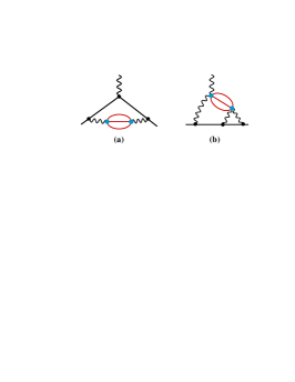
Figure 1: Hadronic contributions to $(g-2)_{\upmu}$: (a) HVP, (b) HLbL.

Here we consider yet another approach to a data-driven evaluation of hadronic contributions rooted in dispersion theory. It is based on sum rules for Compton scattering, of which a famous example is the Gerasimov-Drell-Hearn (GDH) sum rule Gerasimov ; DH66 ; Hosoda :

$$\frac{\alpha}{m^{2}}\varkappa^{2}=\frac{1}{2\pi^{2}}\int_{\nu_{0}}^{\infty}\!\mathrm{d}\nu\,\frac{\sigma_{3/2}(\nu)-\sigma_{1/2}(\nu)}{\nu}\,.$$ (1)

On the left-hand side (lhs), we have $\alpha=e^{2}/4\pi\simeq 1/137$ the fine-structure constant and $\varkappa$ the AMM of the spin-1/2 target particle with mass $m$, whereas the rhs contains the helicity-difference cross section of total photo-absorption on that particle, integrated over the photon energy $\nu$, starting from the photo-absorption threshold $\nu_{0}$.

This is the sort of relation we are looking for: the cross sections can in principle be measured in hadronic channels separately (e.g., $\gamma\mu\to\pi^{0}\mu$) and hence we can “measure” the hadronic contributions to $\varkappa$. Unfortunately, this strategy would not work here, because the sum rule involves $\varkappa^{2}$ and thus we would be probing a very tiny number — recall that the hadronic contribution to $\varkappa_{\upmu}$ is of the order $10^{-8}$. In powers of $\alpha$, the hadronic contribution to $\varkappa_{\upmu}$ starts at $O(\alpha^{2})$, therefore the lhs of the GDH sum rule is $O(\alpha^{5})$, whereas the cross sections of hadronic photo-production starts at $O(\alpha^{3})$. This means there is a huge (at least 5 orders of magnitude) cancellation under the GDH integral, and therefore these cross sections would need to be measured with unprecedented accuracy.

The same $\varkappa^{2}$ feature prevents this sum rule from being useful in theoretical calculations: to compute $\varkappa$ to $O(\alpha^{n})$ one needs to know the cross sections to $O(\alpha^{2n+1})$, which in fact is a more difficult calculation. This was explicitly demonstrated by Dicus and Vega DiV01 , who reproduced the Schwinger’s correction ($\alpha/2\pi$) through the GDH sum rule. Taking a derivative of the GDH sum rule with respect to $\varkappa$ linearizes the sum rule and hence simplifies the calculations Pascalutsa:2004ga ; Holstein:2005db . The drawback of the GDH-derivative method is that the rhs loses a direct connection to experimental observables: the helicity-difference cross section is replaced by a derivative quantity which cannot be accessed in experiment.

Therefore, in what follows we focus on a sum rule which is linear in the AMM and involves an observable cross-section quantity.

II The Schwinger sum rule

Consider the following relation, referred to as the Schwinger sum rule Schwinger:1975ti ; HarunarRashid:1976qz :

$$\varkappa=\frac{m^{2}}{\pi^{2}\alpha}\int_{\nu_{0}}^{\infty}\!\mathrm{d}\nu\,\left[\frac{\sigma_{LT}(\nu,Q^{2})}{Q}\right]_{Q^{2}=0},$$ (2)

where $\sigma_{LT}(\nu,Q^{2})$ — the longitudinal-transverse photo-absorption cross section — is an observable (response function) corresponding to an absorption of a polarized virtual photon with energy $\nu$ and space-like virtuality $Q^{2}$ on the target with mass $m$ and AMM $\varkappa$, whereby the spin of the target flips. This response function is rather common in the studies of nucleon spin structure via electron scattering. For instance, it plays the central role in the evaluation of the so-called $\delta_{LT}$ polarizability of the proton, and hence in the “$\delta_{LT}$ puzzle” (cf., Ref. Hagelstein:2015egb for a recent review). One can introduce it for the muon as well, and benefit from the fact that the sum rule is linear in $\varkappa$, rather than quadratic. However, before applying it to the muon case, let us briefly see how it comes about.

The Schwinger sum rule can be viewed as a consequence of the Burkhardt-Cottingham (BC) and GDH sum rules; in fact, a linear combination of those. Introducing the spin-structure functions $g_{1}(x,Q^{2})$ and $g_{2}(x,Q^{2})$ of the spin-1/2 target, with $x=\nicefrac{{Q^{2}}}{{2m\nu}}$ the Bjorken variable, the BC sum rule reads as Burkhardt:1970ti : $\int_{0}^{1}\mathrm{d}x\,g_{2}(x,Q^{2})=0$. Separating the structure functions into the parts accessed in elastic and inelastic electron scattering, the elastic part is expressed in terms of the Dirac and Pauli form factors, $F_{1}(Q^{2})$ and $F_{2}(Q^{2})$:

$$g_{1}^{\mathrm{el}}(x,Q^{2}) = \mbox{$\frac{1}{2}$}F_{1}(Q^{2})\big{[}F_{1}(Q^{2})+F_{2}(Q^{2})]\,\delta(1-x),$$ (3a)

$$g_{2}^{\mathrm{el}}(x,Q^{2}) = -\mbox{$\frac{Q^{2}}{8m^{2}}$}F_{2}(Q^{2})\big{[}F_{1}(Q^{2})+F_{2}(Q^{2})]\,\delta(1-x),\quad$$ (3b)

whereas the inelastic one, $\bar{g}_{i}=g_{i}-g_{i}^{\mathrm{el}}$, can be expressed in terms of the response functions $\sigma_{LT}$ and $\sigma_{TT}\equiv\nicefrac{{1}}{{2}}\,(\sigma_{1/2}-\sigma_{3/2})$; for more details see, e.g., Ref. (Hagelstein:2015egb, , Sec. 5.2):

$$\bar{g}_{1}(x,Q^{2}) = \frac{1}{4\pi^{2}\alpha}\frac{m\nu^{3}}{\nu^{2}+Q^{2}}\left[\frac{Q}{\nu}\sigma_{LT}+\sigma_{TT}\right],$$ (4a)

$$\bar{g}_{2}(x,Q^{2}) = \frac{1}{4\pi^{2}\alpha}\frac{m\nu^{3}}{\nu^{2}+Q^{2}}\left[\frac{\nu}{Q}\sigma_{LT}-\sigma_{TT}\right].$$ (4b)

In the limit of $Q^{2}\to 0$, with $F_{1}(0)=1$ and $F_{2}(0)=\varkappa$, the BC sum rule yields:

$$(1+\varkappa)\varkappa = \lim_{Q^{2}\to 0}\frac{8m^{2}}{Q^{2}}\int_{0}^{x_{0}}\mathrm{d}x\,\bar{g}_{2}(x,Q^{2}),$$ (5)

$$= \frac{m^{2}}{\pi^{2}\alpha}\int_{\nu_{0}}^{\infty}\mathrm{d}\nu\left[\frac{\sigma_{LT}}{Q}-\frac{\sigma_{TT}}{\nu}\right]_{Q^{2}=0},$$

where $x_{0}=\nicefrac{{Q^{2}}}{{2m\nu_{0}}}$ is the inelastic threshold of the Bjorken variable. Now, the GDH sum rule allows us to cancel the $\varkappa^{2}$ on the lhs against the $\sigma_{TT}$ term on the rhs, resulting in Eq. (2). The latter can also be rewritten in terms of the spin structure functions as:

$$\varkappa=\lim_{Q^{2}\to 0}\frac{8m^{2}}{Q^{2}}\int_{0}^{x_{0}}\mathrm{d}x\;[\bar{g}_{1}+\bar{g}_{2}](x,Q^{2}).$$ (6)

Thus, we “only” need to know how (a moment of) the muon spin-structure function combination $g_{1}+g_{2}$ is affected by hadronic contributions.

III Hadronic contributions via the sum rule

Let us now examine the hadronic contributions to $(g-2)_{\upmu}$ using the Schwinger sum rule. The first thing to consider is the hadron production on the muon shown in Fig. 2, i.e., $\gamma\mu\to\mu+\mathrm{hadrons}$. Examples of these processes are: $\gamma\mu^{\pm}\to\pi^{0}\mu^{\pm}$, $\gamma\mu^{\pm}\to\pi^{+}\pi^{-}\mu^{\pm}$. Here one can distinguish two mechanisms, timelike Compton scattering [Fig. 2(a)], and the Primakoff effect [Fig. 2(b)]. They add up incoherently (i.e., there is no interference term) because of $C$-parity conservation, viz., Furry’s theorem.

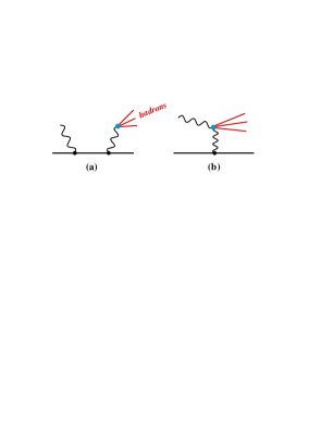
Figure 2: Mechanisms of hadron photo-production off a lepton: (a) timelike Compton scattering (crossed diagram omitted), (b) Primakoff effect.

Both mechanisms begin to contribute at $O(\alpha^{3})$ to $\sigma_{LT}$ and hence at $O(\alpha^{2})$ to $g-2$. The first mechanism (timelike CS) corresponds with the HVP contribution [Fig. 1(a)], and thus provides an alternative access to it, see Sec. III.1. On the other hand, the leading-order contribution of the Primakoff mechanism to $g-2$ should vanish exactly, as it does not correspond with the HVP contribution, and there is no other hadronic contribution to $g-2$ at this order. An explicit proof of this statement [i.e., vanishing effect of Fig. 2(b) on $g-2$] should be possible through the use of the light-by-light scattering sum rules Pascalutsa:2010sj ; Pascalutsa:2012pr . As a result, the Primakoff mechanism can only contribute in interference with subleading effects, such as the one shown in Fig. 3 for the case of $\pi^{0}\gamma$ and $\pi^{0}$ production.

The main advantage of using the Schwinger sum rule, however, is that one need not be concerned with computing the subleading effects of hadronic production — they all can in principle be measured experimentally. This can be achieved at an electron-muon collider with polarized beams needed to access the spin structure functions. Tagging is not necessary, since we only need the quasi-real-photon limit. No separation of radiative corrections is necessary: as long as hadrons are present in the final state, they are part of the hadronic contributions to the spin structure functions of one of the leptons. In fixed-target experiments, one would need to measure the recoil electron polarization.

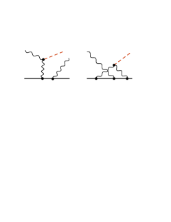
Figure 3: Subleading mechanisms accompanying the single-meson photo-production.

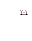
Figure 4: The HLbL contribution to Compton scattering.

Figure 5: Tree-level Compton scattering diagrams.

Apart from the abovementioned hadron-production channels, the muon structure functions can be affected by hadrons in the loops. The most important (in orders of $\alpha$) is the effect of HLbL on the Compton scattering (CS), shown in Fig. 4, interfering with the tree-level Compton effect, Fig. 5. Note that here the initial photon is quasi-real, whereas the final one is real. Thus, the evaluation of the HLbL contribution to $\sigma_{LT}$ involves the HLbL amplitude with only two virtual photons. This is substantially simpler than the corresponding HLbL contribution to $g-2$ shown in Fig. 1(b), which involves the LbL amplitude with three virtual photons and one quasi-real.

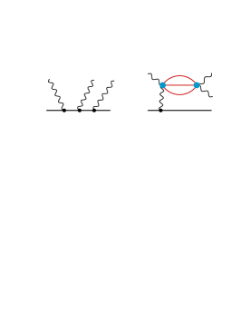
Figure 6: The HLbL contribution through two-photon production.

Another HLbL effect, of the same order in $\alpha$, arises from the interference of the diagrams in Fig. 6, describing the hadronic contribution to the $\mu\gamma\gamma$ channel. Here the treatment of the HLbL contribution is even simpler than in the Compton channel, since the HLbL amplitude is not in the loop and only one of the four photons is virtual.

Before considering these hadronic contributions further, it is instructive to compute the leading QED contribution of Fig. 5 by itself. A straightforward calculation yields:

$$\sigma^{\gamma\mu\to\gamma\mu}_{LT}(\nu,Q^{2})=\frac{\pi\alpha^{2}Q\,(s-m^{2})^{2}}{4m^{3}\nu^{2}\big{(}\nu^{2}+Q^{2}\big{)}}$$ (7)

$$\times\left(-2-\frac{m(m+\nu)}{s}+\frac{3m+2\nu}{\sqrt{\nu^{2}+Q^{2}}}\,\mathrm{arccoth}\frac{m+\nu}{\sqrt{\nu^{2}+Q^{2}}}\right),$$

with $s=m^{2}+2m\nu-Q^{2}$. Substituting this expression into the Schwinger sum rule, one obtains for $\varkappa$ the Schwinger correction: $\alpha/2\pi$. This exercise thus provides a check of the sum rule in leading-order QED, similar to the one done by Tsai et al. Tsai:1975tj .

III.1 Hadronic vacuum polarization

To reproduce the leading HVP contribution [Fig. 1(a)] through the hadron photo-production mechanism shown in Fig. 2(a), we factorize the invariant mass distribution $\mathrm{d}\sigma(\gamma\mu\to\mu X)/\mathrm{d}M_{X}^{2}$, arising from Fig. 2(a), into the cross sections of timelike Compton scattering $\sigma(\gamma\mu\to\gamma^{\ast}\mu)$ and of the subsequent photon decay into hadrons $\Gamma(\gamma^{\ast}\to X)$, cf. Appendix A. The latter cross section is, by unitarity, expressed via the absorptive part of the hadronic contribution to vacuum polarization, $\operatorname{Im}\Pi^{\mathrm{had}}(q^{\prime\,2})$. The tree-level $LT$ cross section of Compton scattering, with initial and final photon virtualities respectively given by $q^{2}=-Q^{2}$ and $q^{\prime\,2}=M^{2}_{X}$, is easily computed to yield:

$$\left[\frac{\sigma^{\gamma\mu\to\gamma^{\ast}\mu}_{LT}(\nu,Q^{2})}{Q}\right]_{Q^{2}=0}=\frac{\pi\alpha^{2}}{2m^{2}\nu^{3}}$$ (8)

$$\qquad\times\,\Big{[}-(5s+m^{2}+M_{X}^{2})\lambda+(s+2m^{2}-2M_{X}^{2})\log\frac{\beta+\lambda}{\beta-\lambda}\Big{]},$$

with $s=m^{2}+2m\nu$, $\beta=(s+m^{2}-M_{X}^{2})/2s$, and $\lambda=(1/2s)\sqrt{[s-(m+M_{X})^{2}]\,[s-(m-M_{X})^{2}]}$. From the Schwinger sum rule we then have:

$$\varkappa = \frac{m^{2}}{\pi^{2}\alpha}\int\limits_{4m_{\pi}^{2}}^{\infty}\mathrm{d}M_{X}^{2}\int\limits_{\nu_{0}}^{\infty}\!\mathrm{d}\nu\,\left[\frac{1}{Q}\frac{\mathrm{d}\sigma^{\gamma\mu\to\mu X}_{LT}(\nu,Q^{2})}{\mathrm{d}M^{2}_{X}}\right]_{Q^{2}=0}=\frac{1}{\pi}\int\limits_{4m_{\pi}^{2}}^{\infty}\mathrm{d}M_{X}^{2}\,\frac{\operatorname{Im}\Pi^{\mathrm{had}}(M_{X}^{2})}{M_{X}^{2}}\frac{m^{2}}{\pi^{2}\alpha}\int\limits_{\nu_{0}}^{\infty}\!\mathrm{d}\nu\,\left[\frac{\sigma^{\gamma\mu\to\gamma^{\ast}\mu}_{LT}(\nu,Q^{2})}{Q}\right]_{Q^{2}=0}$$ (9)

where $\nu_{0}=M_{X}(1+M_{X}^{2}/2m^{2})$ is the photo-production threshold, while $4m_{\pi}^{2}$ is set by the lightest produced state (here, $\pi^{-}\pi^{+}$ pair). Finally, performing the integration over $\nu$, we obtain:

$$\frac{m^{2}}{\pi^{2}\alpha}\int_{\nu_{0}}^{\infty}\!\mathrm{d}\nu\,\left[\frac{\sigma^{\gamma\mu\to\gamma^{\ast}\mu}_{LT}(\nu,Q^{2})}{Q}\right]_{Q^{2}=0}\,=\,\frac{\alpha}{\pi}K(M_{X}^{2}/m^{2})\,\equiv\,\frac{\alpha}{\pi}\int_{0}^{1}\mathrm{d}x\frac{x^{2}(1-x)}{x^{2}+(1-x)(M_{X}^{2}/m^{2})},$$ (10)

and hence the standard expression for the HVP contribution (see, e.g., Ref. Jegerlehner:2017gek ),

$$\varkappa^{\mathrm{HVP}}=\frac{\alpha}{\pi^{2}}\int_{4m_{\pi}^{2}}^{\infty}\mathrm{d}s\,K(s/m^{2})\,\frac{\operatorname{Im}\Pi^{\mathrm{had}}(s)}{s},$$ (11)

is exactly reproduced.

In practice, a determination of the HVP contribution through the Schwinger sum rule has an important conceptual difference from the standard practice of measuring $e^{+}e^{-}\to\mathrm{hadrons}$. The latter method involves an approximation of the single-photon exchange, the two-photon exchange effects ought to be removed. In the sum-rule method, the two-photon-exchange and other subleading effects need not be removed, they are part of the sought hadronic contribution.

Further novel features of calculating the hadronic contributions through the Schwinger sum rule can be seen in the following example of the meson-exchange contribution.

III.2 Pseudoscalar meson contribution

The neutral pseudoscalar mesons $\pi^{0}$ and $\eta$ play a significant role in the HLbL contribution through the mechanism shown in Fig. 7. Let us see how this mechanism is evaluated using the Schwinger sum rule.

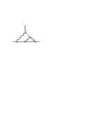
Figure 7: $\pi^{0}$-exchange HLbL contribution to $(g-2)_{\upmu}$.

In the hadronic channel, we need to know the $LT$ cross section for the single-meson photo-production off the lepton. This can in principle be measured directly, or calculated to leading-order evaluating the diagrams in Fig. 8. Note that, in addition to the Primakoff mechanism (last diagram), we have here the subleading (in $\alpha$) mechanisms of the type given by the second diagram of Fig. 3. The latter is effectively accounted for in the first two graphs in Fig. 8, where the meson-lepton-lepton ($\pi\ell\ell$) coupling is fixed from the decay width of pseudoscalar mesons into leptons (i.e., $\pi^{0}\to e^{+}e^{-}$ and $\eta\to\mu^{+}\mu^{-}$).

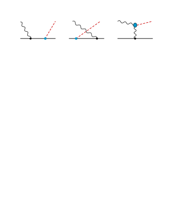
Figure 8: Single-meson photo-production off a lepton.

The same experimental information on pseudoscalar-into-leptons decays fixes the counter-term needed to renormalize the vertex calculation of the form factor in Fig. 9, which is needed in the Compton channel calculation, cf. Fig. 10(a). It is interesting that this $\pi\ell\ell$ form factor enters profoundly in the calculation of $\pi^{0}$ exchange in the hyperfine splitting of muonic hydrogen Hagelstein:2015lph ; Huong:2015naj ; Dorokhov2017 ; Hagelstein:2017cbl . The $\pi^{0}$ effects in $(g-2)_{\upmu}$ and muonic hydrogen are thus interrelated.

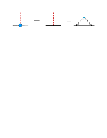
Figure 9: Pseudoscalar meson coupling to leptons.

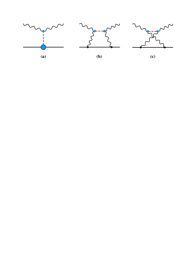
Figure 10: Pseudoscalar-meson contribution to Compton scattering (a) $t$-channel exchange with the $\pi\ell\ell$ form factor given by Fig. 9; (b) and (c) show the direct and crossed box, respectively. Drawn using Jaxodraw Binosi:2003yf .

Furthermore, there are contributions from the $2\gamma$ and $\pi^{0}\gamma$ channels given respectively by Fig. 6 with $\pi^{0}$ as the virtual hadronic state and the first diagram of Fig. 3.

It is important to realize that calculating the $\pi^{0}$ contribution through the diagrams in Figs. 8 and 10 and the multi-particle channels, we do not need the transition form factor (TFF) with two virtual photons. We only need the TFF for a single virtual photon [i.e, $F_{\pi^{0}\gamma\gamma^{\ast}}(Q^{2})$] in the box graphs of Fig. 10(b) and (c), since the external photons are (quasi-)real. The doubly-virtual TFFs could be used in evaluation of the $\pi\ell\ell$ form factor Fig. 9. However, their impact therein is largely diminished by the renormalization and the use of the empirical width.

IV Conclusion

We have considered the hadronic contributions (HVP and HLbL) to $g-2$, and showed how they can be assessed using the Schwinger sum rule presented in Sec. II. The sum rule separates the hadronic contributions into two types:

• hadron photo-production (Fig. 2),

• HLbL contribution to non-hadronic channels (Fig. 4, 6).

Type (i) has a clear relation to observables. These are the spin structure functions of the lepton with hadrons in the final state (hadronic channels) that could in principle be measured in electron-muon collisions. This type of contributions is readily suited for a model-independent, “data-driven” evaluation.

In type (ii), the hadrons may appear in the loops, similar to the sought HLbL contribution to $g-2$ [Fig. 1(b)]. However, the sum rule evaluation only requires the HLbL for the situation of two virtual photons forming a loop, rather than three virtual photons forming two loops as required in the direct evaluation of Fig. 1(b). The former evaluation, therefore, requires much less information about HLbL, and is technically simpler. For example, the evaluation of the neutral-pion, and other single-meson contributions, will only require the transition form factor to one real and one virtual photon ($M\to\gamma\gamma^{\ast}$), rather than two virtual photons ($M\to\gamma^{\ast}\gamma^{\ast}$) as required usually.

The Schwinger sum rule is thus a very promising tool for a data-driven evaluation of the hadronic contributions to $(g-2)_{\upmu}$. Despite being quite different from the existing dispersive approaches, the present approach may benefit from the dispersive analysis of the HLbL amplitude by Colangelo et al. Colangelo:2014pva ; Colangelo:2014dfa ; Colangelo:2017qdm ; Colangelo:2017fiz , trimmed to the narrower kinematical range required for the evaluation of Fig. 4. In a more distant perspective, the type (ii) contribution will be calculable in lattice QCD.

In Sec. III.1, we have reproduced the standard expression for the HVP contribution via the sum rule. In Sec. III.2, we have outlined how the sum rule program works for the pseudoscalar meson contributions. With very few modifications it applies, of course, to the axion contributions to $g-2$, which have lately been receiving renewed attention in connection with collider searches Marciano:2016yhf ; Bauer:2017nlg .

The advantages of evaluating the axion and other beyond-SM contributions by using the Schwinger sum rule are less obvious than in the hadronic case, where data-driven approaches are generally desirable in the absence of precise ab initio calculations. And, even in a more advanced lattice-QCD era, the presented sum-rule approach may be advantageous, if only for its clear-cut separation of the explicit hadron production from the virtual hadronic effects.

Appendix A Factorizing the hadron photo-production through timelike Compton scattering

Here we show how the hadron photo-production process $(\gamma\mu\to\mu X)$, going through the mechanism in Fig. 2(a), can be decomposed into the timelike Compton scattering $(\gamma\mu\to\gamma^{\ast}\mu)$ and the virtual-photon decay into hadrons $(\gamma^{\ast}\to X)$. The factorization applies to all helicity cross sections, including $\sigma_{LT}$. Denoting the incoming (outgoing) muon and photon 4-momenta as $p$ ($p^{\prime}$) and $q$ ($q^{\prime}$), and the 4-momenta of the particles in $X$ as $k_{i}$, the total photo-absorption cross section is given by:

$$\sigma(\gamma\mu\to\mu X)=\frac{(2\pi)^{4}}{4I}\int\mathrm{d}^{4}q^{\prime}\int\prod_{i}\frac{\mathrm{d}^{3}\boldsymbol{k}_{i}}{2E_{k_{i}}(2\pi)^{3}}\int\frac{\mathrm{d}^{3}\boldsymbol{p^{\prime}}}{2E_{p^{\prime}}(2\pi)^{3}}\left[\frac{\Lambda^{\dagger\mu}\Lambda^{\nu}\rho_{\mu\nu}}{(-q^{\prime\,2})^{2}}\right]\delta^{4}(q^{\prime}-\sum_{i}k_{i})\,\delta^{4}(p+q-p^{\prime}-q^{\prime}),$$ (12)

with $I^{2}=(p\cdot q)^{2}-p^{2}\,q^{2}$ the initial flux factor, $\Lambda^{\mu}$ the virtual-photon decay vertex, and $\rho^{\mu\nu}$ the squared matrix element of the timelike Compton scattering, where the vector indices refer to the virtual photon. The integration over $q^{\prime}$ is conveniently introduced at the expense of inserting a compensating $\delta$-function. The other integrations cover the phase space of the final state to form a total cross section.

The photon decay width is defined as:

$$\left[\Gamma(\gamma^{\ast}\to X)\right]^{\mu\nu} = \int\prod_{i}\frac{\mathrm{d}^{3}\boldsymbol{k_{i}}}{2E_{k_{i}}(2\pi)^{3}}\frac{\Lambda^{\dagger\mu}\Lambda^{\nu}}{2E_{q^{\prime}}}(2\pi)^{4}\delta^{4}(q^{\prime}-\sum_{i}k_{i}),$$ (13a)

$$= -\frac{1}{\sqrt{q^{\prime\,2}}}\,(q^{\prime\,2}g^{\mu\nu}-q^{\prime\mu}q^{\prime\nu})\operatorname{Im}\Pi_{X}(q^{\prime\,2}),$$ (13b)

where in the last step we made use of its transverse tensor structure and unitarity, with $\Pi_{X}$ being the contribution of state $X$ to the vacuum polarization.

Substituting Eq. (13) into Eq. (12), and using gauge invariance ($q^{\prime\mu}\rho_{\mu\nu}=0$) to drop the $q^{\prime\mu}q^{\prime\nu}$ term in Eq. (13b), we find:

$$\sigma(\gamma\mu\to\mu X)=-\frac{1}{2I}\int\mathrm{d}^{4}q^{\prime}\int\frac{\mathrm{d}^{3}\boldsymbol{p^{\prime}}}{2E_{p^{\prime}}(2\pi)^{3}}\,\rho^{\mu}_{\mu}\,\frac{\operatorname{Im}\Pi_{X}(q^{\prime\,2})}{q^{\prime\,2}}\,\delta^{4}(p+q-p^{\prime}-q^{\prime}).$$ (14)

Now we can identify the total cross section of the timelike Compton scattering, $\sigma(\gamma\mu\to\gamma^{\ast}\mu)$, and thus arrive at:

$$\sigma(\gamma\mu\to\mu X)=\frac{1}{\pi}\int\frac{\mathrm{d}M_{X}^{2}}{M_{X}^{2}}\,\sigma(\gamma\mu\to\gamma^{\ast}\mu)\operatorname{Im}\Pi_{X}(M_{X}^{2}).$$ (15)

The remaining integral over $M_{X}^{2}=q^{\prime\,2}$ reflects the fact that we are integrating over all possible states $X$.

References

- (1) T. Blum, A. Denig, I. Logashenko, E. de Rafael, B. Lee Roberts, T. Teubner and G. Venanzoni, arXiv:1311.2198 (2013) [hep-ph].
- (2) M. Benayoun et al., arXiv:1407.4021 (2014) [hep-ph].
- (3) I. Logashenko et al. [Muon g-2 Collaboration], J. Phys. Chem. Ref. Data 44, no. 3, 031211 (2015).
- (4) G. Venanzoni [Fermilab E989 Collaboration], Nucl. Part. Phys. Proc. 273-275, 584 (2016) [arXiv:1411.2555 [physics.ins-det]].
- (5) T. Blum, S. Chowdhury, M. Hayakawa and T. Izubuchi, Phys. Rev. Lett. 114, 012001 (2015) [arXiv:1407.2923 [hep-lat]].
- (6) T. Blum, N. Christ, M. Hayakawa, T. Izubuchi, L. Jin and C. Lehner, Phys. Rev. D 93, no. 1, 014503 (2016) [arXiv:1510.07100 [hep-lat]].
- (7) J. Green, O. Gryniuk, G. von Hippel, H. B. Meyer and V. Pascalutsa, Phys. Rev. Lett. 115, no. 22, 222003 (2015) [arXiv:1507.01577 [hep-lat]].
- (8) J. Green, N. Asmussen, O. Gryniuk, G. von Hippel, H. B. Meyer, A. Nyffeler and V. Pascalutsa, PoS LATTICE 2015, 109 (2016) [arXiv:1510.08384 [hep-lat]].
- (9) F. Jegerlehner, Springer Tracts Mod. Phys. 274 (2017).
- (10) M. Davier, Nucl. Part. Phys. Proc. 287-288, 70 (2017) [arXiv:1612.02743 [hep-ph]].
- (11) G. Colangelo, M. Hoferichter, B. Kubis, M. Procura and P. Stoffer, Phys. Lett. B 738, 6 (2014) [arXiv:1408.2517 [hep-ph]].
- (12) G. Colangelo, M. Hoferichter, M. Procura and P. Stoffer, JHEP 1409, 091 (2014) [arXiv:1402.7081 [hep-ph]].
- (13) G. Colangelo, M. Hoferichter, M. Procura and P. Stoffer, Phys. Rev. Lett. 118, no. 23, 232001 (2017) [arXiv:1701.06554 [hep-ph]].
- (14) G. Colangelo, M. Hoferichter, M. Procura and P. Stoffer, JHEP 1704, 161 (2017) [arXiv:1702.07347 [hep-ph]].
- (15) V. Pauk and M. Vanderhaeghen, Phys. Rev. D 90, 113012 (2014) [arXiv:1409.0819 [hep-ph]].
- (16) S. B. Gerasimov, Sov. J. Nucl. Phys. 2, 430 (1966) [Yad. Fiz. 2, 598 (1966)].
- (17) S. D. Drell and A. C. Hearn, Phys. Rev. Lett. 16, 908 (1966).
- (18) M. Hosoda and K. Yamamoto, Prog. Theor. Phys. 36, 425 (1966); ibid. 426 (1966).
- (19) D.A. Dicus and R. Vega, Phys. Lett. B 501, 44 (2001).
- (20) V. Pascalutsa, B. R. Holstein and M. Vanderhaeghen, Phys. Lett. B 600, 239 (2004).
- (21) B. R. Holstein, V. Pascalutsa and M. Vanderhaeghen, Phys. Rev. D 72, 094014 (2005) [hep-ph/0507016].
- (22) J. S. Schwinger, Proc. Nat. Acad. Sci. 72, 1 (1975); ibid. 72, 1559 (1975) [Acta Phys. Austriaca Suppl. 14, 471 (1975)].
- (23) A. M. Harun ar-Rashid, Nuovo Cim. A 33, 447 (1976).
- (24) F. Hagelstein, R. Miskimen and V. Pascalutsa, Prog. Part. Nucl. Phys. 88, 29 (2016) [arXiv:1512.03765 [nucl-th]].
- (25) H. Burkhardt and W. N. Cottingham, Annals Phys. 56, 453 (1970).
- (26) V. Pascalutsa and M. Vanderhaeghen, Phys. Rev. Lett. 105, 201603 (2010) [arXiv:1008.1088 [hep-ph]].
- (27) V. Pascalutsa, V. Pauk and M. Vanderhaeghen, Phys. Rev. D 85, 116001 (2012) [arXiv:1204.0740 [hep-ph]].
- (28) W. y. Tsai, L. L. DeRaad, Jr. and K. A. Milton, Phys. Rev. D 11, 3537 (1975); Erratum: Phys. Rev. D 13, 1144 (1976).
- (29) F. Hagelstein and V. Pascalutsa, PoS CD 15, 077 (2016) [arXiv:1511.04301 [nucl-th]].
- (30) N. T. Huong, E. Kou and B. Moussallam, Phys. Rev. D 93, no. 11, 114005 (2016) [arXiv:1511.06255 [hep-ph]].
- (31) A. E. Dorokhov, N. I. Kochelev, A. P. Martynenko, F. A. Martynenko and R. N. Faustov, Phys. Part. Nucl. Lett. 14, 857 (2017) [arXiv:1704.07702 [hep-ph]].
- (32) F. Hagelstein, PhD thesis (University of Mainz, 2017) [arXiv:1710.00874 [nucl-th]].
- (33) D. Binosi and L. Theussl, Comput. Phys. Commun. 161, 76 (2004) [hep-ph/0309015].
- (34) W. J. Marciano, A. Masiero, P. Paradisi and M. Passera, Phys. Rev. D 94, no. 11, 115033 (2016) [arXiv:1607.01022 [hep-ph]].
- (35) M. Bauer, M. Neubert and A. Thamm, Phys. Rev. Lett. 119, no. 3, 031802 (2017) [arXiv:1704.08207 [hep-ph]].