Abstract We introduce uncertainty regions to perform inference on partial correlations when data are missing not at random. These uncertainty regions are shown to have a desired asymptotic coverage. Their finite sample performance is illustrated via simulations and real data example.

Keywords. Nonignorable dropout; uncertainty region; change - change analysis; brain markers; cognition.

1 Introduction

This paper proposes methods to perform inference on partial correlations when data are missing not at random. The motivation for this work comes from a recent investigation of the relationship between longitudinal changes in brain structure, e.g. gray matter volume of hippocampus, and changes in cognition, e.g. episodic memory, when adjusting for the effect of age and hypertension, see Gorbach et al. (2017). A partial correlation coefficient may be used to describe an association between two random variables, such as changes in brain and cognition, that is not due to other related covariates, for example age and hypertension (see Anderson (1958) for theory and Nilsson et al. (1997), Marrelec et al. (2006), Van Petten et al. (2004) for application). However, a natural feature of most longitudinal investigations is the occurrence of missing data due to dropout. In Gorbach et al. (2017), for example, measures of the episodic memory change could be obtained for each individual, while 41% of data on the gray matter volume changes was missing due to dropout. Moreover, individuals with more pronounced health and brain deterioration are expected to drop out from longitudinal investigations earlier than healthier subjects. Thus the probability of an observation to be missing is expected to depend on its unobserved value (data missing not at random).

Some work has been devoted to inference on partial correlation when data are missing. D’Angelo et al. (2012), for example, considered an EM algorithm and multiple imputation for the case of trivariate normal distribution with data missing at random. Gorbach et al. (2017) inferred on statistical significance of partial correlation allowing for data missing not at random. This was done using the relationship between the partial correlation and a regression parameter in combination with results developed by Genbäck et al. (2015). This approach does not allow, however, to construct uncertainty regions for partial correlations but only to perform significance testing.

In this paper we consider the situation when the data is missing not at random. To model the dependency between variables (which are not observed for all individuals) and the probability that their observations are missing, we introduce a parameter $\gamma$ which is typically unknown in applications. We then construct confidence intervals (with given coverage (1-$\alpha$)100%) for a partial correlation of interest for each plausible value of the parameter $\gamma$ based on asymptotic results. We then propose to use the union of these confidence intervals, which we call uncertainty region, and prove that this region has at least (1-$\alpha$)100% coverage asymptotically.

This paper is organized as follows. Partial correlation and its relation to a regression parameter are briefly introduced in Section 2. The missing data mechanisms we consider are described in Section 3. Section 4 presents our results and introduces uncertainty regions for each missing data mechanisms, while Section 5 illustrates the application of the method to the aforementioned longitudinal study of the relation between changes in brain structure and cognition. A simulation study is conducted in Section 6, followed by concluding remarks in Section 7.

2 Partial correlation

The partial correlation between random variables $X_{1}$ and $X_{2}$ while adjusting for $X_{3},\ldots,X_{p}$ is defined as the correlation between residuals of the projections of $X_{1}$ and $X_{2}$ on the linear space spanned by $X_{3},\ldots,X_{p}$. Let $X_{1},\ldots,X_{p}$ be random variables with finite second moments, $EX_{j}^{2}<\leavevmode\nobreak\ \infty,$ $j=1,\ldots,p$, and consider the projections of $X_{1}$ and $X_{2}$ on the linear spaces spanned by $X_{2},\ldots,X_{p}$ and $X_{3},\ldots,X_{p}$ respectively:

$$\begin{split}&X_{1}=\beta_{1}+\beta_{2}X_{2}+\ldots+\beta_{p}X_{p}+\xi_{1},\\ &X_{2}=\theta_{1}+\theta_{2}X_{3}+\ldots+\theta_{p-1}X_{p}+\xi_{2},\end{split}$$ (2.1)

where $\mathrm{E}\xi_{i}=0$, $\text{Cov}(\xi_{i},{X}_{j})=0,\ i=1,2,\ j=3,\ldots,p$ and $\text{Cov}(\xi_{1},X_{2})=0.$ We will assume that $\sigma^{2}_{2.3\ldots p}=\mathrm{Var}(\xi_{2})\neq 0$ and $\sigma^{2}_{1.2\ldots p}=\mathrm{Var}(\xi_{1})\neq 0.$ From (2.1) we have that $X_{1}=(\beta_{1}+\beta_{2}\theta_{1})+(\beta_{2}\theta_{2}+\beta_{3})X_{3}+\ldots+(\beta_{2}\theta_{p-1}+\beta_{p})X_{p}+\beta_{2}\xi_{2}+\xi_{1}$ and $\text{Cov}(\xi_{1},\xi_{2})=0$.

The partial correlation $\rho$ between $X_{1}$ and $X_{2}$ while adjusting for $X_{3},\ldots,X_{p}$ is then $\rho=\text{Corr}(\xi_{2},\beta_{2}\xi_{2}+\xi_{1})$ and can be expressed as

$$\rho=\frac{\beta_{2}}{\sqrt{\beta_{2}^{2}+\sigma^{2}_{1.2\ldots p}/\sigma^{2}_{2.3\ldots p}}}.$$ (2.2)

We use representation (2.2) in the sequel.

3 Missing data mechanisms (MDM)

We consider three models where the data on $X_{1}$ or $X_{1}$ and $X_{2}$ are missing not at random (MNAR).

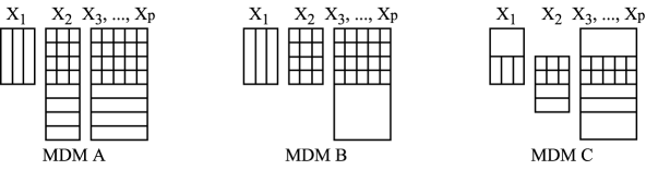
Figure 1: Data patterns. Vertical shading represents data used for estimation of $\beta_{2}$ and $\sigma^{2}_{1.2\ldots p}$, horizontal shading represents data used for estimation of $\sigma^{2}_{2.3\ldots p}$. Grid shading corresponds to data used for estimation of $\beta_{2}$, $\sigma^{2}_{1.2\ldots p}$ and $\sigma^{2}_{2.3\ldots p}.$ Empty boxes represent the observed data that is not used in the estimation procedures.

MDM A. Let $X_{2},X_{3},\ldots,X_{p}$ be fully observed while $X_{1}$ is observed if $Z=1$ and missing otherwise (see Figure 1), where

$$Z=\mathbbm{1}(\boldsymbol{X}_{\text{-}1}\boldsymbol{\delta}+\eta_{1}>0),$$ (3.1)

$\boldsymbol{X}_{\text{-}1}=(1,X_{2},\ldots,X_{p})$, $\boldsymbol{\delta}$ is a $p$ column vector of unknown parameters, $\eta_{1}\sim\mathcal{N}(0,1)$ and $\mathbbm{1}$ is the indicator function. In order to introduce missing not at random data in $X_{1}$ we follow Genbäck et al. (2015) by modeling $\xi_{1}$ in (2.1) as $\xi_{1}=\leavevmode\nobreak\ \gamma\sigma_{1.2\ldots p}\eta_{1}+\epsilon,$ where $\mathrm{E}\epsilon=0,$ $\eta_{1}\rotatebox[origin={c}]{90.0}{$\models$}(X_{2},\ldots,X_{p}),$ $\epsilon\rotatebox[origin={c}]{90.0}{$\models$}(X_{2},\ldots,X_{p},\eta_{1})$ and $\models$ denotes independence between random variables. Then $\gamma\neq 0$ corresponds to MNAR data, while data are missing at random (MAR) when $\gamma=0.$
MDM B. Let $X_{3},\ldots,X_{p}$ be fully observed while $X_{1}$ and $X_{2}$ are observed if $Z=1$ and missing otherwise (see Figure 1), where

$$Z=\mathbbm{1}(\boldsymbol{X}_{\text{-}12}\boldsymbol{\delta}+\eta_{1}>0),$$ (3.2)

$\boldsymbol{X}_{\text{-}12}=(1,X_{3},\ldots,X_{p}),$ $\boldsymbol{\delta}$ is a $(p-1)$ column vector of unknown parameters, $\eta_{1}\sim\mathcal{N}(0,1).$ We introduce missing not at random data in $X_{1}$ by modeling $\xi_{1}$ in (2.1) as $\xi_{1}=\leavevmode\nobreak\ \gamma\sigma_{1.2\ldots p}\eta_{1}+\epsilon,$ where $\mathrm{E}\epsilon=0,$ $\eta_{1}\rotatebox[origin={c}]{90.0}{$\models$}(X_{2},\ldots,X_{p}),$ $\epsilon\rotatebox[origin={c}]{90.0}{$\models$}(X_{2},\ldots,X_{p},\eta_{1})$, $\xi_{2}\rotatebox[origin={c}]{90.0}{$\models$}(X_{3},\ldots,X_{p},\eta_{1}).$ Then $\gamma\neq 0$ corresponds to MNAR data for $X_{1}$, while data on $X_{1}$ are MAR when $\gamma=0$.
MDM C. Let $X_{3},\ldots,X_{p}$ be fully observed while $X_{1}$ is observed if $Z_{1}=1$ and missing otherwise, $X_{2}$ is observed if $Z_{2}=1$ and missing otherwise (see Figure 1), where

$$Z_{1}=\mathbbm{1}(\boldsymbol{X}_{\text{-}12}\boldsymbol{\delta}_{1}+\eta_{1}>0),$$ (3.3)

$$Z_{2}=\mathbbm{1}(\boldsymbol{X}_{\text{-}12}\boldsymbol{\delta}_{2}+\eta_{2}>0),$$ (3.4)

$\boldsymbol{X}_{\text{-}12}=(1,X_{3},\ldots,X_{p}),$ $\boldsymbol{\delta}_{1}$ and $\boldsymbol{\delta}_{2}$ are $(p-1)$ column vectors of unknown parameters and $(\eta_{1},\eta_{2})\sim\mathcal{N}(\boldsymbol{0},\boldsymbol{I}_{2})$, $\boldsymbol{I}_{2}$ is an identity matrix of size 2. As above we introduce missing not at random data by modeling $\xi_{1}$ and $\xi_{2}$ in (2.1) as $\xi_{1}=\gamma_{1}\sigma_{1.2\ldots p}\eta_{1}+\epsilon_{1}$, $\xi_{2}=\gamma_{2}\sigma_{2.3\ldots p}\eta_{2}+\epsilon_{2}$, where $\mathrm{E}\epsilon_{1}=0$, $\mathrm{E}\epsilon_{2}=0,$ $\eta_{1}\rotatebox[origin={c}]{90.0}{$\models$}(X_{2},\ldots,X_{p},\eta_{2}),$ $\epsilon_{1}\rotatebox[origin={c}]{90.0}{$\models$}(X_{2},\ldots,X_{p},\eta_{1},\eta_{2}),$ $\eta_{2}\rotatebox[origin={c}]{90.0}{$\models$}(X_{3},\ldots,X_{p})$ , $\epsilon_{2}\rotatebox[origin={c}]{90.0}{$\models$}(X_{3},\ldots,X_{p},\eta_{2}).$ $\gamma_{1}\neq 0$ corresponds to MNAR data for $X_{1}$ and $\gamma_{2}\neq 0$ corresponds to MNAR data for $X_{2}.$

4 Inference

4.1 Inference under MDM A

Let $\{X_{1i},X_{2i},\ldots,X_{pi},Z_{i}\}_{i=1}^{N}$ be a random sample from $(X_{1},X_{2},\ldots,X_{p},Z)$ for which MDM A holds. For a given $\gamma,$ we propose an estimator $\widehat{\rho}_{\gamma}$ for $\rho$ based on bias correction of complete cases ordinary least squares (OLS) estimators of quantities in (2.2) (see Figure 1):

$$\widehat{\rho}_{\gamma}=\frac{\widehat{\beta}_{2}}{\sqrt{\widehat{\beta}_{2}^{2}+\widehat{\sigma}_{1.2\ldots p}^{2}/\widehat{\sigma}^{2}_{2.3\ldots p}}},$$ (4.1)

where

$$\widehat{\beta}_{2}=\widehat{\beta}_{2,ols}-\gamma\widehat{\sigma}_{1.2\ldots p}\left[(\boldsymbol{X}_{\text{-}1s}^{T}\boldsymbol{X}_{\text{-}1s})^{\text{-}1}\boldsymbol{X}_{\text{-}1s}^{T}\boldsymbol{\lambda}_{\widehat{\boldsymbol{u}}}\right]_{2},$$

$$\widehat{\sigma}_{1.2\ldots p}^{2}=\frac{\widehat{\sigma}_{1.2\ldots p,ols}^{2}}{1+\gamma^{2}(\boldsymbol{\widehat{u}}^{T}\boldsymbol{\lambda}_{\widehat{\boldsymbol{u}}}-\boldsymbol{\lambda}_{\widehat{\boldsymbol{u}}}^{T}\boldsymbol{X}_{\text{-}1s}(\boldsymbol{X}_{\text{-}1s}^{T}\boldsymbol{X}_{\text{-}1s})^{\text{-}1}\boldsymbol{X}_{\text{-}1s}^{T}\boldsymbol{\lambda}_{\widehat{\boldsymbol{u}}})/(n-p)},$$ (4.2)

and $\widehat{\sigma}^{2}_{2.3\ldots p}$ is an OLS estimator of $\sigma^{2}_{2.3\ldots p}$ based on $\{X_{2i},\ldots,X_{pi}\}_{i=1}^{N}.$
Here $\widehat{\beta}_{2,ols}=\left[(\boldsymbol{X}_{\text{-}1s}^{T}\boldsymbol{X}_{\text{-}1s})^{\text{-}1}\boldsymbol{X}_{\text{-}1s}^{T}\boldsymbol{X}_{1s}\right]_{2}$ and $\widehat{\sigma}_{1.2\ldots p,ols}^{2}=\boldsymbol{X}_{1s}^{T}(\boldsymbol{I}_{n}-\boldsymbol{X}_{\text{-}1s}(\boldsymbol{X}_{\text{-}1s}^{T}\boldsymbol{X}_{\text{-}1s})^{\text{-}1}\boldsymbol{X}_{\text{-}1s}^{T})\boldsymbol{X}_{1s}/(n-p)$ are OLS estimators of $\beta_{2}$ and $\sigma_{1.2\ldots p}^{2}$ based on $n$ complete cases; $\boldsymbol{X}_{1s}$ denotes an $n<N$ vector of observed $X_{1}$ for complete cases; $\boldsymbol{X}_{\text{-}1s}$ represents an $n\times p$ matrix of observed covariates $(1,X_{2},\ldots,X_{p})$ for complete cases. $\boldsymbol{\widehat{u}}=(\widehat{u}_{1},\ldots,\widehat{u}_{n})^{T}=-\boldsymbol{X}_{\text{-}1s}\widehat{\boldsymbol{\delta}}$, $\widehat{\boldsymbol{\delta}}$ is the maximum likelihood estimator of $\boldsymbol{\delta}$ in probit model (3.1) based on full data $\{X_{2i},\ldots,X_{pi},Z_{i}\}_{i=1}^{N}$; $\boldsymbol{\lambda_{\widehat{u}}}=(\lambda(\widehat{u}_{1}),\ldots,\lambda(\widehat{u}_{n}))^{T}$, $\lambda(\widehat{u}_{i})=\frac{\phi(\widehat{u}_{i})}{\Phi(-\widehat{u}_{i})},\ i=1,\ldots,n$ denotes the inverse Mills ratio, $\phi$ and $\Phi$ are respectively the standard normal density and cumulative distribution functions. Also, $\boldsymbol{I}_{n}$ is an $n\times n$ identity matrix and $[v]_{2}$ denotes the second element of a vector $v.$

Theorem 4.1.

Under MDM A and regularity assumptions (see Appendix A) $\widehat{\rho}_{\gamma}$ is a consistent estimator of $\rho$ and

$$\sqrt{n}(\widehat{\rho}_{\gamma}-\rho)/\widehat{\text{se}}_{\widehat{\rho}_{\gamma}}\rightarrow_{d}\mathcal{N}(0,1),$$

where $\widehat{\text{se}}_{\widehat{\rho}_{\gamma}}=\sqrt{\frac{\widehat{\sigma}_{1.2\ldots p}^{2}(1+\gamma^{2}\boldsymbol{\widehat{u}}^{T}\boldsymbol{\lambda}_{\boldsymbol{\widehat{u}}}/n-\gamma^{2}\boldsymbol{\lambda}_{\boldsymbol{\widehat{u}}}^{T}\boldsymbol{\lambda}_{\boldsymbol{\widehat{u}}}/n)(\boldsymbol{X}_{\text{-}1s}^{T}\boldsymbol{X}_{\text{-}1s})_{22}^{\text{-}1}}{\widehat{\beta}^{2}_{2}+\widehat{\sigma}^{2}_{1.2\ldots p}/\widehat{\sigma}^{2}_{2.3\ldots p}}}.$

A proof is provided in Appendix A. A $(1-\alpha)100\%$ confidence interval for $\rho$ is thus:

$$\text{CI}(\rho,\gamma,\alpha)=[\widehat{\rho}_{\gamma}-c_{\frac{\alpha}{2}}\widehat{\text{se}}_{\widehat{\rho}_{\gamma}};\widehat{\rho}_{\gamma}+c_{\frac{\alpha}{2}}\widehat{\text{se}}_{\widehat{\rho}_{\gamma}}].$$ (4.3)

Here $c_{\frac{\alpha}{2}}$ is the $(1-\alpha)100\text{th}$ percentile of the standard normal distribution. However, the true value of $\gamma,$ $\gamma_{0},$ is typically unknown in applications. Setting it to one certain value in analysis, for example 0, is a strong assumption which is typically difficult to check empirically. Instead we propose to assume that $\gamma_{0}$ belongs to an interval $[\gamma_{min},\gamma_{max}]$ and provide inference under this weaker assumption. For example, since $\gamma$ is the correlation between $\xi_{1}$ and $\eta_{1},$ $\gamma_{0}\in[-1,1].$ Then, intervals (4.3) can be constructed for each $\gamma\in[\gamma_{min},\gamma_{max}]$. Although each specific confidence interval (4.3) may fail to cover the true $\rho_{0}$ corresponding to $\gamma_{0}$ with probability $(1-\alpha)100\%,$ their union

$$\text{UR}(\rho,[\gamma_{min},\gamma_{max}],\alpha)=\bigcup\limits_{\gamma\in[\gamma_{min},\gamma_{max}]}\text{CI}(\rho,\gamma,\alpha),$$

which we call the uncertainty region for $\rho$, covers $\rho_{0}$ with at least $(1-\alpha)100\%$ probability as can be seen below.

Corollary 4.1.1.

Under the assumptions of Theorem 4.1, if the true $\gamma_{0}\in[\gamma_{min},\gamma_{max}]$, the uncertainty region $\text{UR }(\rho,[\gamma_{min},\gamma_{max}],\alpha)$ has asymptotic coverage for $\rho_{0}$ of at least $(1-\alpha)100\%.$

A proof is provided in Appendix A.

4.2 Inference under MDM B

Results under missing mechanisms B follow the same structure as for mechanism A. A consistent and asymptotically normal estimator for partial correlation (see Appendix B, Theorem B.1) is defined by (4.1), with $\boldsymbol{\widehat{u}}=(\widehat{u}_{1},\ldots,\widehat{u}_{n})^{T}=-\boldsymbol{X}_{\text{-}12s}\widehat{\boldsymbol{\delta}}$, where $\boldsymbol{X}_{\text{-}12s}$ represents an $n\times(p-1)$ matrix of observed covariates $(1,X_{3},\ldots,X_{p})$ for complete cases; $\widehat{\boldsymbol{\delta}}$ a maximum likelihood estimator of $\boldsymbol{\delta}$ in probit model (3.2) based on full data $\{X_{3i},\ldots,X_{pi},Z_{i}\}_{i=\leavevmode\nobreak\ 1}^{N},$ and $\widehat{\sigma}^{2}_{2.3\ldots p}$ is an ordinary OLS estimator of $\sigma^{2}_{2.3\ldots p}$ based on complete cases $\{X_{2i},\ldots,X_{pi}\}_{i=1}^{n}$. Uncertainty regions can then be constructed as above for MDM A (see Appendix B, Corollary B.1.1).

4.3 Inference under MDM C

Let $\{X_{1i},X_{2i},\ldots,X_{pi},Z_{1i},Z_{2i}\}_{i=1}^{N}$ be a random sample from $(X_{1},X_{2},\ldots,X_{p},Z_{1},Z_{2})$ for which MDM C holds. Results under MDM C follow the same structure as for mechanism A. A consistent and asymptotically normal estimator for $\rho$ (see Appendix B, Theorem B.2 for proofs) is defined as

$$\widehat{\rho}_{\gamma_{1},\gamma_{2}}=\frac{\widehat{\beta}_{2}}{\sqrt{\widehat{\beta}_{2}^{2}+\widehat{\sigma}_{1.2\ldots p}^{2}/\widehat{\sigma}_{2.3\ldots p}^{2}}},$$

where

$$\widehat{\beta}_{2}=\widehat{\beta}_{2,ols}-\gamma\widehat{\sigma}_{1.2\ldots p}\left[(\boldsymbol{X}_{\text{-}1s}^{T}\boldsymbol{X}_{\text{-}1s})^{\text{-}1}\boldsymbol{X}_{\text{-}1s}^{T}\boldsymbol{\lambda}_{\widehat{\boldsymbol{u}}}\right]_{2},$$

$$\widehat{\sigma}_{1.2\ldots p}^{2}=\frac{\widehat{\sigma}_{1.2\ldots p,ols}^{2}}{1+\gamma_{1}^{2}(\boldsymbol{\widehat{u}}^{T}\boldsymbol{\lambda}_{\widehat{\boldsymbol{u}}}-\boldsymbol{\lambda}_{\widehat{\boldsymbol{u}}}^{T}\boldsymbol{X}_{\text{-}1s}(\boldsymbol{X}_{\text{-}1s}^{T}\boldsymbol{X}_{\text{-}1s})^{\text{-}1}\boldsymbol{X}_{\text{-}1s}^{T}\boldsymbol{\lambda}_{\widehat{\boldsymbol{u}}})/(n-p)},$$

$$\widehat{\sigma}_{2.3\ldots p}^{2}=\frac{\widehat{\sigma}_{2.3\ldots p,ols}^{2}}{1+\gamma_{2}^{2}(\boldsymbol{\widehat{w}}^{T}\boldsymbol{\lambda}_{\widehat{\boldsymbol{w}}}-\boldsymbol{\lambda}_{\widehat{\boldsymbol{w}}}^{T}\boldsymbol{X}_{\text{-}12s_{2}}(\boldsymbol{X}_{\text{-}12s_{2}}^{T}\boldsymbol{X}_{\text{-}12s_{2}})^{\text{-}1}\boldsymbol{X}_{\text{-}12s_{2}}^{T}\boldsymbol{\lambda}_{\widehat{\boldsymbol{w}}})/(n_{2}-p)},$$

$\widehat{\beta}_{2,ols}=\left[(\boldsymbol{X}_{\text{-}1s}^{T}\boldsymbol{X}_{\text{-}1s})^{\text{-}1}\boldsymbol{X}_{\text{-}1s}^{T}\boldsymbol{X}_{1s}\right]_{2}$ and $\widehat{\sigma}_{1.2\ldots p,ols}^{2}=\boldsymbol{X}_{1s}^{T}(\boldsymbol{I}_{n}-\boldsymbol{X}_{\text{-}1s}(\boldsymbol{X}_{\text{-}1s}^{T}\boldsymbol{X}_{\text{-}1s})^{\text{-}1}\boldsymbol{X}_{\text{-}1s}^{T})\boldsymbol{X}_{1s}/(n-p)$ are OLS estimators of $\beta_{2}$ and $\sigma_{1.2\ldots p}^{2}$ based on $n$ complete cases, and
$\widehat{\sigma}_{2.3\ldots p,ols}^{2}=\boldsymbol{X}_{2s_{2}}^{T}(\boldsymbol{I}_{n_{2}}-\boldsymbol{X}_{\text{-}12s_{2}}(\boldsymbol{X}_{\text{-}12s}^{T}\boldsymbol{X}_{\text{-}12s_{2}})^{\text{-}1}\boldsymbol{X}_{\text{-}12s_{2}}^{T})\boldsymbol{X}_{2s_{2}}/(n_{2}-p)$ is an OLS estimator of $\sigma_{2.3\ldots p}^{2}$ based on $n_{2}$ cases with observed $X_{2}$. $\boldsymbol{X}_{\text{-}1s}$ and $\boldsymbol{X}_{\text{-}12s}$ represent respectively an $n\times p$ and an $n\times(p-1)$ matrices of observed covariates $(1,X_{2},\ldots,X_{p})$ and $(1,X_{3},\ldots,X_{p})$ for complete cases; $\boldsymbol{X}_{\text{-}12s_{2}}$ is an $n_{2}\times(p-1)$ matrix of observed covariates $(1,X_{3},\ldots,X_{p})$ for cases with observed $X_{2}$. $\boldsymbol{X}_{1s}$ denotes an $n$ vector of observed $X_{1}$ for complete cases, $\boldsymbol{X}_{2s_{2}}$ is an $n_{2}$ vector of observed $X_{2}$. $\boldsymbol{\lambda_{\widehat{u}}}=(\lambda(\widehat{u}_{1}),\ldots,\lambda(\widehat{u}_{n}))^{T},$ where $\lambda$ denotes inverse Mills ratio, $\boldsymbol{\widehat{u}}=(\widehat{u}_{1},\ldots,\widehat{u}_{n})^{T}=-\boldsymbol{X}_{\text{-}12s}\widehat{\boldsymbol{\delta}}_{1}$, $\widehat{\boldsymbol{\delta}}_{1}$ is the maximum likelihood estimator of $\boldsymbol{\delta}_{1}$ under model (3.3) based on full data $\{X_{3i},\ldots,X_{pi},Z_{1i}\}_{i=\leavevmode\nobreak\ 1}^{N}.$ $\boldsymbol{\lambda_{\widehat{w}}}=(\lambda(\widehat{w}_{1}),\ldots,\lambda(\widehat{w}_{n_{2}}))^{T}$, where $\lambda$ denotes inverse Mills ratio, $\boldsymbol{\widehat{w}}=(\widehat{w}_{1},\ldots,\widehat{w}_{n_{2}})^{T}=-\boldsymbol{X}_{\text{-}12s_{2}}\widehat{\boldsymbol{\delta}}_{2}$, $\widehat{\boldsymbol{\delta}}_{2}$ is the maximum likelihood estimator of $\boldsymbol{\delta}_{2}$ under probit model (3.4) based on full data $\{X_{3i},\ldots,X_{pi},Z_{2i}\}_{i=\leavevmode\nobreak\ 1}^{N}.$ A $(1-\alpha)100\%$ confidence interval is

$$\text{CI}(\rho,\gamma_{1},\gamma_{2},\alpha)=[\widehat{\rho}_{\gamma_{1},\gamma_{2}}-c_{\frac{\alpha}{2}}\widehat{\text{se}}_{\widehat{\rho}_{\gamma_{1},\gamma_{2}}};\widehat{\rho}_{\gamma_{1},\gamma_{2}}+c_{\frac{\alpha}{2}}\widehat{\text{se}}_{\widehat{\rho}_{\gamma_{1},\gamma_{2}}}].$$

Here $c_{\frac{\alpha}{2}}$ is the $(1-\alpha)100\%$ percentile of the standard normal distribution and

$$\widehat{\text{se}}_{\widehat{\rho}_{\gamma_{1},\gamma_{2}}}=\sqrt{\frac{\widehat{\sigma}_{1.2\ldots p}^{2}(1+\gamma_{1}^{2}\boldsymbol{\widehat{u}}^{T}\boldsymbol{\lambda}_{\boldsymbol{\widehat{u}}}/n-\gamma_{1}^{2}\boldsymbol{\lambda}_{\boldsymbol{\widehat{u}}}^{T}\boldsymbol{\lambda}_{\boldsymbol{\widehat{u}}}/n)(\boldsymbol{X}_{\text{-}1s}^{T}\boldsymbol{X}_{\text{-}1s})_{22}^{\text{-}1}}{\widehat{\beta}_{2}^{2}+\widehat{\sigma}_{1.2\ldots p}^{2}/\widehat{\sigma}_{2.3\ldots p}^{2}}}.$$

An uncertainty region is, accordingly,

$$\text{UR}(\rho,[\gamma_{1min},\gamma_{1max}],[\gamma_{2min},\gamma_{2max}],\alpha)=\bigcup\limits_{\gamma_{1}\in[\gamma_{1min},\gamma_{1max}],\gamma_{2}\in[\gamma_{2min},\gamma_{2max}]}\text{CI}(\rho,\gamma_{1},\gamma_{2},\alpha),$$

and asymptotically covers the true $\rho=\rho_{\gamma_{10},\gamma_{20}}$, where $(\gamma_{10},\gamma_{20})$ is the true value of $(\gamma_{1},\gamma_{2})$, with at least $(1-\alpha)100\%$ probability (see Appendix B, Corollary B.2.1).

5 Application

We use the theoretical results developed in this paper to infer on partial correlation between longitudinal changes in gray matter volume of hippocampus and episodic memory decline, when adjusting for the effect of age and hypertension (Gorbach et al., 2017), with the data from the Betula study (Nilsson et al., 1997). Briefly, the sample consists of 264 older adults that underwent magnetic resonance imaging (MRI) at one of the Betula waves, had up to 25 years history of cognitive assessment and were scheduled for a MRI follow-up. Of the 264 initially scanned participants, 155 underwent a follow-up MRI examination; see Gorbach et al. (2017) for more detailed description of the sample and measures used. Since information on cognition changes could be obtained for all individuals while changes in gray matter volume of hippocampus are missing for approximately 41% of individuals in the sample, we consider missing data mechanism A. Point estimates $\widehat{\rho}_{\gamma}$ can be constructed under assumptions of the true $\gamma_{0}=\gamma$, where $\gamma\in[0;1]$. $\gamma$ is constrained to be nonnegative, since given age, hypertension and cognition change, an individual with smaller value of gray matter change, that is fraction of gray matter volume at second and first measurements, may be expected to have poorer health and thus more likely to drop out, which corresponds to $\gamma\geq 0$. As can be seen from Figure 2, an uncertainty region for the partial correlation is $UR(\rho,[0;1],0.05)=[0.153;0.511].$ The interval does not contain 0 which is in line with the analysis in Gorbach et al. (2017) where an uncertainty region for $\rho$ could not be produced.

Figure 2: Estimated partial correlation between changes of gray matter volume of hippocampus and episodic memory changes controlled for age and hypertension (solid line) for different values of parameter $\gamma$ with corresponding 95% CI’s (bounds of CI’s are represented as dashed curves) in presence of missing not at random data.

6 Simulation study

This simulation study uses a design inspired by the above application. Observations for age ($X_{3}$) and hypertension ($X_{4}$) are simulated from the empirical distribution of the data. Since in the study episodic memory change ($X_{2}$) was available for the full sample, while hippocampus gray matter change ($X_{1}$) was partially observed, we simulate data under missing mechanism A as follows:

$$X_{2i} =2.313-0.042X_{3i}-0.216X_{4i}+\xi_{2i},$$

$$X_{1i} =1.092+0.01X_{2i}-0.002X_{3i}-0.006X_{4i}+0.028\gamma_{0}\eta_{1i}+\epsilon_{i},$$

$$Z_{i} =\mathbbm{1}(2.708+0.548X_{2i}-0.036X_{3i}-0.042X_{4i}+\eta_{1i}>0),$$

$$(\xi_{2i},\epsilon_{i},\eta_{1i}) \sim N_{3}\left(\boldsymbol{0},\text{diag}(1.16,0.028^{2}(1-\gamma^{2}),1)\right),i=1,\ldots,N,$$

where regression parameters for simulation of $X_{2i}$ and $X_{1i}$ are the corresponding OLS estimates from complete cases linear regressions fit obtained from the data. $Z_{i}$ is simulated from the probit regression fit to the data where we have changed the parameter for $X_{2i}$ from 0.048 to 0.548 to increase the difference between complete cases and full data distributions. The partial correlation between simulated hippocampus change and episodic memory decline is $\rho=0.359.$ Data are generated for $\gamma_{0}=0.1,0.5,0.8$ and for sample sizes $N=100$ and $N=250$. Around 50% of data are missing for each generated sample. The width and empirical coverage of 95% confidence intervals based on complete cases (CC CI), confidence intervals constructed under the true data law $\gamma=\gamma_{0}$ (oracle CI) and uncertainty regions $UR(\rho,[0,0.5],0.05)$ are computed for 1000 replicates.

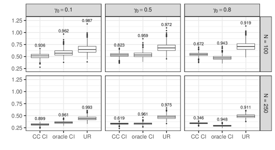
Figure 3: Boxplots of widths of the intervals for 95% nominal coverage for complete cases confidence intervals (CC CI), CI under the true data law ($\gamma=\gamma_{0}$, oracle CI) and URs assuming that $\gamma\in[0,0.5]$ for 1000 simulations of data using $\gamma_{0}=0.1,0.5,0.8$ and for sample sizes $N=100$ and $N=250$. Empirical coverage is labeled above each boxplot.

As Figure 3 shows, the empirical coverage of complete cases confidence intervals decreases with increasing value of $\gamma$ and/or increasing sample size. The empirical coverage of oracle confidence intervals based on true data law is around 95% as expected. The empirical coverage of constructed uncertainty regions, in turn, is as expected above 95% when $\gamma_{0}$ used for data generation lies within the assumed in estimation interval $[0,0.5]$ (for the cases $\gamma_{0}=0.1$ and $\gamma_{0}=0.5$). Noteworthy, even for the data generated under $\gamma_{0}=0.8$, uncertainty regions constructed under the assumption of $\gamma_{0}\in[0,0.5]$ have much higher empirical coverage than complete cases confidence intervals.

7 Discussion

The uncertainty regions proposed here are an alternative to establishing possible identifiability of $\gamma$ and the partial correlation in the considered semiparametric missing mechanism models. Known methods for estimation in this constext are Heckman two-step type approaches (Heckman, 1979; Vella, 1998), which rely heavily on the nonlinearity of the inverse Mills ratio. However, as the inverse Mills ratio is linear for a wide range of its arguments, identifiability and thus point estimation is not possible in practice (Puhani, 2000).

Uncertainty regions were studied in wider generality in Vansteelandt et al. (2006), who proposed to construct an uncertainty region for an unidentified parameter by adding confidence limits to estimated bounds of an ignorance region, which is a range of parameter values that correspond to different full data distributions compatible with the observed data law. To do so, Vansteelandt et al. (2006) relies on the assumption of lower and upper bounds of the ignorance region being independent of the observed data law (Assumption 2, p. 960). In our approach, by using instead a union of confidence intervals to define an uncertainty region, one avoids the aforementioned assumption, which is seldom fulfilled.

Genbäck et al. (2015) uses bounds for the variance of the residuals in a linear regression to deduce uncertainty regions for regression parameters when data is missing not at random. The bias corrected estimators of such residual variance introduced in this paper (e.g. (4.2)) can be used to provide narrower uncertainty regions than those proposed in Genbäck et al. (2015).

Finally, note that the results developed in the paper also hold when missing data occur in $X_{3},\ldots,X_{p}$ if the latter is missing at random.

Appendix A

Regularity assumptions for Theorem 4.1.

1. $EX_{j}^{2}<\leavevmode\nobreak\ \infty,\ j=1,\ldots,p;$ $\sigma^{2}_{2.3\ldots p}\neq 0$, $\sigma^{2}_{1.2\ldots p}\neq 0;$

2. $\det\boldsymbol{X}_{\text{-}1s}^{T}\boldsymbol{X}_{\text{-}1s}\neq 0$, $\det\mathrm{E}(\boldsymbol{X}_{\text{-}1}^{T}\boldsymbol{X}_{\text{-}1}|Z=1)\neq 0;$

3. $\det\boldsymbol{X}_{\text{-}12s}^{T}\boldsymbol{X}_{\text{-}12s}\neq 0,\ \det\mathrm{E}(\boldsymbol{X}_{\text{-}12}^{T}\boldsymbol{X}_{\text{-}12})\neq 0,$ where $\boldsymbol{X}_{\text{-}12s}=(\boldsymbol{1},\boldsymbol{X}_{3},\ldots,\boldsymbol{X}_{p})$ - $N\times(p-1)$ matrix of observed covariates and $\boldsymbol{X}_{\text{-}12}=(1,X_{3},\ldots,X_{p})$ is a vector of random variables;

4. $1+\frac{\gamma^{2}}{n-p}(\boldsymbol{\widehat{u}}^{T}\boldsymbol{\lambda}_{\widehat{\boldsymbol{u}}}-\boldsymbol{\lambda}_{\widehat{\boldsymbol{u}}}^{T}\boldsymbol{X}_{\text{-}1s}(\boldsymbol{X}_{\text{-}1s}^{T}\boldsymbol{X}_{\text{-}1s})^{\text{-}1}\boldsymbol{X}_{\text{-}1s}^{T}\boldsymbol{\lambda}_{\widehat{\boldsymbol{u}}})\neq 0$ for all $n$,
   $1+\gamma^{2}\mathrm{E}(u\lambda_{u}|Z=1)-\gamma^{2}\mathrm{E}\left(\boldsymbol{X}_{\text{-}1}\lambda_{u}|Z=1\right)\mathrm{E}^{\text{-}1}(\boldsymbol{X}_{\text{-}1}^{T}\boldsymbol{X}_{\text{-}1}|Z=1)\mathrm{E}(\boldsymbol{X}_{\text{-}1}^{T}\lambda_{u}|Z=1)\neq 0,$ where $u=-\boldsymbol{X}_{\text{-}1}\boldsymbol{\delta}$ and $\lambda_{u}=\frac{\phi(u)}{\Phi(-u)}$, $\lambda$ denotes inverse Mills ratio;

5. $\widehat{\sigma}^{2}_{2.3\ldots p}\neq 0$, and at least one of $\widehat{\beta}_{2}\neq 0$ or $\widehat{\sigma}_{1.2\ldots p}^{2}\neq 0$ for all $n.$

Proof of Theorem 4.1..

$\widehat{\sigma}^{2}_{2.3\ldots p}\rightarrow_{p}\sigma^{2}_{2.3\ldots p}$ as an OLS estimator of $\sigma^{2}_{2.3\ldots p}$ based on $\{X_{2i},\ldots,X_{pi}\}_{i=1}^{N}$ and from regularity assumptions 1, 3.

Proof of the consistency of $\widehat{\sigma}_{1.2\ldots p}^{2}$. Let $\boldsymbol{\xi}_{1s}$ denote an $n\times 1$ vector of $\xi_{1}$ for complete cases. By the law of large numbers, the continuous mapping theorem and regularity assumptions 1, 2,

$$\widehat{\sigma}_{1.2\ldots p,ols}^{2} =\frac{1}{n-p}\boldsymbol{X}_{1s}^{T}(\boldsymbol{I}_{n}-\boldsymbol{X}_{\text{-}1s}(\boldsymbol{X}_{\text{-}1s}^{T}\boldsymbol{X}_{\text{-}1s})^{\text{-}1}\boldsymbol{X}_{\text{-}1s}^{T})\boldsymbol{X}_{1s}=\frac{\boldsymbol{\xi}_{1s}^{T}\boldsymbol{\xi}_{1s}}{n-p}-\frac{\boldsymbol{\xi}_{1s}^{T}\boldsymbol{X}_{\text{-}1s}(\boldsymbol{X}_{\text{-}1s}^{T}\boldsymbol{X}_{\text{-}1s})^{\text{-}1}\boldsymbol{X}_{\text{-}1s}^{T}\boldsymbol{\xi}_{1s}}{n-p}$$

$$\rightarrow_{p}E(\xi_{1}^{2}|Z=1)-E(\xi_{1}\boldsymbol{X}_{\text{-}1}|Z=1)\mathrm{E}^{\text{-}1}(\boldsymbol{X}_{\text{-}1}^{T}\boldsymbol{X}_{\text{-}1}|Z=1)E(\xi_{1}\boldsymbol{X}^{T}_{\text{-}1}|Z=1).$$ (A.1)

Since for MDM A $\mathrm{E}\epsilon=0$, $\eta_{1}\rotatebox[origin={c}]{90.0}{$\models$}(X_{2},\ldots,X_{p})$ and $\epsilon\rotatebox[origin={c}]{90.0}{$\models$}(X_{2},\ldots,X_{p},\eta_{1}),$

$$\mathrm{E}(\xi_{1}^{2}|Z=1) =\gamma^{2}\sigma_{1.2\ldots p}^{2}\text{E}(\eta_{1}^{2}|Z=1)+2\gamma\sigma_{1.2\ldots p}\text{E}(\eta_{1}\epsilon|Z=1)+\text{E}(\epsilon^{2}|Z=1)$$

$$=\gamma^{2}\sigma_{1.2\ldots p}^{2}\mathrm{E}\left[\mathrm{E}(\eta_{1}^{2}|\boldsymbol{X}_{\text{-}1},Z=1)|Z=1\right]+\mathrm{E}\epsilon^{2}=\gamma^{2}\sigma_{1.2\ldots p}^{2}\mathrm{E}(1+u\lambda_{u}|Z=1)+\sigma_{1.2\ldots p}^{2}(1-\gamma^{2}),$$ (A.2)

$$\mathrm{E}(\xi_{1}\boldsymbol{X}_{\text{-}1}|Z=1)=\mathrm{E}\left[\boldsymbol{X}_{\text{-}1}\mathrm{E}(\gamma\sigma_{1.2\ldots p}\eta_{1}+\epsilon|\boldsymbol{X}_{\text{-}1},Z=1)|Z=1\right]=\gamma\sigma_{1.2\ldots p}\mathrm{E}(\boldsymbol{X}_{\text{-}1}\lambda_{u}|Z=1).$$ (A.3)

The last equality in (A.2) follows from the expressions for the variance and the mean of truncated normal distribution (see Heckman (1979)): $\mathrm{E}\left[\mathrm{E}(\eta_{1}^{2}|\boldsymbol{X}_{\text{-}1},Z=1)|Z=1\right]=\mathrm{E}\left[\mathrm{E}(\eta_{1}^{2}|\boldsymbol{X}_{\text{-}1},\eta_{1}>-\boldsymbol{X}_{\text{-}1}\boldsymbol{\delta})|Z=1\right]=\mathrm{E}(1+u\lambda_{u}|Z=1).$ From (A.1), (A.2) and (A.3),

$$\widehat{\sigma}_{1.2\ldots p,ols}^{2}\rightarrow_{p}\sigma_{1.2\ldots p}^{2}\left[1+\gamma^{2}\mathrm{E}(u\lambda_{u}|Z=1)-\gamma^{2}\mathrm{E}\left(\boldsymbol{X}_{\text{-}1}\lambda_{u}|Z=1\right)\mathrm{E}^{\text{-}1}(\boldsymbol{X}_{\text{-}1}^{T}\boldsymbol{X}_{\text{-}1}|Z=1)\mathrm{E}(\boldsymbol{X}_{\text{-}1}^{T}\lambda_{u}|Z=1)\right].$$ (A.4)

Since $\boldsymbol{\widehat{\delta}}$ is the consistent estimator in probit regression, $\widehat{u}_{i}$ and $\lambda_{\widehat{u}_{i}}$ are consistent estimators of $u_{i}$ and $\lambda_{u_{i}}$. $E\lambda^{2}_{u}<\infty$, since similar to Birnbaum (1942) it can be shown that $\forall x\in R$ $\lambda(x)\leq 2|x|+2$. From the regularity assumption 1 by the law of large numbers and the continuous mapping theorem,

$$\boldsymbol{\widehat{u}}^{T}\boldsymbol{\lambda}_{\widehat{\boldsymbol{u}}}/(n-p)=(\boldsymbol{\widehat{u}}^{T}\boldsymbol{\lambda}_{\widehat{\boldsymbol{u}}}-\boldsymbol{u}^{T}\boldsymbol{\lambda}_{\boldsymbol{u}})/(n-p)+\boldsymbol{u}^{T}\boldsymbol{\lambda}_{\boldsymbol{u}}/(n-p)\rightarrow_{p}0+\mathrm{E}(u\lambda_{u}|Z=1),$$ (A.5)

$$\boldsymbol{\lambda}_{\widehat{\boldsymbol{u}}}^{T}\boldsymbol{X}_{\text{-}1s}(\boldsymbol{X}_{\text{-}1s}^{T}\boldsymbol{X}_{\text{-}1s})^{\text{-}1}\boldsymbol{X}_{\text{-}1s}^{T}\boldsymbol{\lambda}_{\widehat{\boldsymbol{u}}}/(n-p)\rightarrow_{p}\mathrm{E}\left(\boldsymbol{X}_{\text{-}1}\lambda_{u}|Z=1\right)\mathrm{E}^{\text{-}1}(\boldsymbol{X}_{\text{-}1}^{T}\boldsymbol{X}_{\text{-}1}|Z=1)\mathrm{E}(\boldsymbol{X}_{\text{-}1}^{T}\lambda_{u}|Z=1).$$ (A.6)

From (A.4), (A.5), (A.6), regularity assumption 4 and the continuous mapping theorem

$$\widehat{\sigma}_{1.2\ldots p}^{2}\rightarrow_{p}\sigma_{1.2\ldots p}^{2}.$$ (A.7)

Consistency of $\widehat{\beta}_{2}$ follows from the law of large numbers, the continuous mapping theorem, regularity assumptions 1, 2 and (A.3):

$$\widehat{\beta}_{2}= (\boldsymbol{X}_{\text{-}1s}^{T}\boldsymbol{X}_{\text{-}1s})^{\text{-}1}\boldsymbol{X}_{\text{-}1s}^{T}[\boldsymbol{X}_{1s}-\gamma\widehat{\sigma}_{1.2\ldots p}\boldsymbol{\lambda}_{\widehat{\boldsymbol{u}}}]e_{2}$$

$$\rightarrow_{p}\left[\mathrm{E}^{\text{-}1}(\boldsymbol{X}_{\text{-}1}^{T}\boldsymbol{X}_{\text{-}1}|Z=1)\left(\mathrm{E}(\boldsymbol{X}_{\text{-}1}^{T}\boldsymbol{X}_{\text{-}1}\boldsymbol{\beta}|Z=1)+\mathrm{E}(\boldsymbol{X}_{\text{-}1}^{T}\xi_{1}|Z=1)-\gamma\sigma_{1.2\ldots p}\mathrm{E}(\boldsymbol{X}_{\text{-}1}^{T}\boldsymbol{\lambda}_{\boldsymbol{u}}|Z=1)\right)\right]_{2}=\beta_{2},$$ (A.8)

where $\boldsymbol{\beta}=(\beta_{1},\ldots,\beta_{p})^{T}.$

Asymptotic normality of $\widehat{\beta}_{2}$ follows from Slutsky’s and the multivariate central limit theorem,

$$\sqrt{n}(\widehat{\beta}_{2}-\beta_{2}) =\sqrt{n}\left[(\boldsymbol{X}^{T}_{\text{-}1s}\boldsymbol{X}_{\text{-}1s})^{\text{-}1}[\boldsymbol{X}^{T}_{\text{-}1s}\boldsymbol{\xi}_{1s}-\gamma\widehat{\sigma}_{1.2\ldots p}\boldsymbol{X}_{\text{-}1s}^{T}\boldsymbol{\lambda}_{\widehat{\boldsymbol{u}}}]\right]_{2}$$

$$\rightarrow_{d}\mathcal{N}\left(0,\left[\mathrm{E}^{\text{-}1}(\boldsymbol{X}_{\text{-}1}^{T}\boldsymbol{X}_{\text{-}1}|Z=1)\mathrm{Var}(\boldsymbol{X}^{T}_{\text{-}1}(\xi_{1}-\gamma\sigma_{1.2\ldots p}\lambda_{u})|Z=1)\mathrm{E}^{\text{-}1}(\boldsymbol{X}_{\text{-}1}^{T}\boldsymbol{X}_{\text{-}1}|Z=1)^{T}\right]_{22}\right).$$

From the properties of truncated normal distribution,

$$\mathrm{Var}(\boldsymbol{X}^{T}_{\text{-}1}(\xi_{1}-\gamma\sigma_{1.2\ldots p}\lambda_{u})|Z=1)= \mathrm{E}\left(\boldsymbol{X}^{T}_{\text{-}1}\mathrm{Var}(\xi_{1}-\gamma\sigma_{1.2\ldots p}\lambda_{u}|\boldsymbol{X}_{\text{-}1},Z=1)\boldsymbol{X}_{\text{-}1}|Z=1\right)$$

$$+\mathrm{Var}\left(\mathrm{E}(\boldsymbol{X}^{T}_{\text{-}1}\boldsymbol{X}_{\text{-}1}|Z=1)\boldsymbol{\beta}\right)$$

$$= \mathrm{E}\left(\boldsymbol{X}^{T}_{\text{-}1}\left[\gamma^{2}\sigma_{1.2\ldots p}^{2}\mathrm{Var}(\eta_{1}|\boldsymbol{X}_{\text{-}1},Z=1)+\mathrm{Var}(\epsilon|\boldsymbol{X}_{\text{-}1},Z=1)\right]\boldsymbol{X}_{\text{-}1}|Z=1\right)$$

$$= \mathrm{E}\left(\boldsymbol{X}^{T}_{\text{-}1}\left[\gamma^{2}\sigma_{1.2\ldots p}^{2}(1+u\lambda_{u}-\lambda_{u}^{2})+\sigma_{1.2\ldots p}^{2}(1-\gamma^{2})\right]\boldsymbol{X}_{\text{-}1}|Z=1\right)$$

$$= \sigma_{1.2\ldots p}^{2}\mathrm{E}\left(\boldsymbol{X}^{T}_{\text{-}1}\boldsymbol{X}_{\text{-}1}\left[(1+\gamma^{2}u\lambda_{u}-\gamma^{2}\lambda_{u}^{2})\right]|Z=1\right).$$

Therefore,

$$\sqrt{n}(\widehat{\beta}_{2}-\beta_{2})\rightarrow_{d}\mathcal{N}\left(0,\nu_{\beta_{2}}\right)$$ (A.9)

$$\nu_{\beta_{2}}=\sigma_{1.2\ldots p}^{2}[\mathrm{E}^{\text{-}1}(\boldsymbol{X}_{\text{-}1}^{T}\boldsymbol{X}_{\text{-}1}|Z=1)\mathrm{E}\left(\boldsymbol{X}^{T}_{\text{-}1}\boldsymbol{X}_{\text{-}1}\left[(1+\gamma^{2}u\lambda_{u}-\gamma^{2}\lambda_{u}^{2})\right]|Z=1\right)\mathrm{E}^{\text{-}1}(\boldsymbol{X}_{\text{-}1}^{T}\boldsymbol{X}_{\text{-}1}|Z=1)^{T}]_{22}.$$

From the consistency of $\widehat{\sigma}_{2.3\ldots p}^{2}$, (A.7), (A.8), regularity assumption 5 and the continuous mapping theorem, $\widehat{\rho}_{\gamma}\rightarrow_{p}\rho$. Using additionally (A.9) and Slutsky’s theorem, it follows that

$$\sqrt{n}(\widehat{\rho}_{\gamma}-\rho)\rightarrow_{d}\mathcal{N}\left(0,\frac{\nu_{\beta_{2}}}{\beta^{2}_{2}+\sigma^{2}_{1.2\ldots p}/\sigma^{2}_{2.3\ldots p}}\right).$$

Consistency of $\widehat{\text{se}}_{\widehat{\rho}_{\gamma}}$ follows from the law of large numbers and the continuous mapping theorem:

$$\widehat{\text{se}}_{\widehat{\rho}_{\gamma}}^{2}=\frac{\widehat{\sigma}_{1.2\ldots p}^{2}(1+\gamma^{2}\boldsymbol{\widehat{u}}^{T}\boldsymbol{\lambda}_{\boldsymbol{\widehat{u}}}/n-\gamma^{2}\boldsymbol{\lambda}_{\boldsymbol{\widehat{u}}}^{T}\boldsymbol{\lambda}_{\boldsymbol{\widehat{u}}}/n)(\boldsymbol{X}_{\text{-}1s}^{T}\boldsymbol{X}_{\text{-}1s})_{22}^{\text{-}1}}{\widehat{\beta}_{2}^{2}+\widehat{\sigma}_{1.2\ldots p}^{2}/\widehat{\sigma}^{2}_{2.3\ldots p}}\rightarrow_{p}\frac{\nu_{\beta_{2}}}{\beta^{2}_{2}+\sigma^{2}_{1.2\ldots p}/\sigma^{2}_{2.3\ldots p}}.$$

Therefore,

$$\sqrt{n}(\widehat{\rho}_{\gamma}-\rho)/\widehat{\text{se}}_{\widehat{\rho}_{\gamma}}\rightarrow_{d}\mathcal{N}(0,1).$$

∎

Proof of Corollary 4.1.1.

Let denote $\Gamma=[\gamma_{min},\gamma_{max}].$

$$\text{pr}\left(\rho_{0}\in UR(\rho,\Gamma,\alpha\right) =\text{pr}\left(\rho_{0}\in\bigcup\limits_{\gamma\in\Gamma}\text{CI}(\rho,\gamma,\alpha)\right)=1-\text{pr}\left(\rho_{0}\notin\bigcup\limits_{\gamma\in\Gamma}\text{CI}(\rho,\gamma,\alpha)\right)$$

$$=1-\text{pr}\left(\rho_{0}\in\bigcap\limits_{\gamma\in\Gamma}(-\infty,\widehat{\rho}_{\gamma}-c_{\frac{\alpha}{2}}\widehat{\text{se}}_{\widehat{\rho}_{\gamma}})\cup(\widehat{\rho}_{\gamma}+c_{\frac{\alpha}{2}}\widehat{\text{se}}_{\widehat{\rho}_{\gamma}},\infty)\right)$$

$$=1-\text{pr}(\bigcap\limits_{\gamma\in\Gamma}\{\widehat{\rho}_{\gamma}-c_{\frac{\alpha*}{2}}\widehat{\text{se}}_{\widehat{\rho}_{\gamma}}>\rho_{0}\})-\text{pr}(\bigcap\limits_{\gamma\in\Gamma}\{\widehat{\rho}_{\gamma}+c_{\frac{\alpha*}{2}}\widehat{\text{se}}_{\widehat{\rho}_{\gamma}}<\rho_{0}\})$$

$$\geq 1-\text{pr}(\widehat{\rho}_{\gamma_{0}}-c_{\frac{\alpha*}{2}}\widehat{\text{se}}_{\widehat{\rho}_{\gamma_{0}}}>\rho_{0})-\text{pr}(\widehat{\rho}_{\gamma_{0}}+c_{\frac{\alpha*}{2}}\widehat{\text{se}}_{\widehat{\rho}_{\gamma_{0}}}<\rho_{0})$$ (A.10)

$$=\text{pr}(\widehat{\rho}_{\gamma_{0}}-c_{\frac{\alpha*}{2}}\widehat{\text{se}}_{\widehat{\rho}_{\gamma_{0}}}<\rho_{0}<\widehat{\rho}_{\gamma_{0}}+c_{\frac{\alpha*}{2}}\widehat{\text{se}}_{\widehat{\rho}_{\gamma_{0}}})\rightarrow 1-\alpha,\ n\rightarrow\infty$$

from the definition of CI. (A.10) follows since $\bigcap\limits_{\gamma\in\Gamma}\{\widehat{\rho}_{\gamma}-c_{\frac{\alpha*}{2}}\widehat{\text{se}}_{\widehat{\rho}_{\gamma}}>\rho_{0}\}\subset\{\widehat{\rho}_{\gamma_{0}}-c_{\frac{\alpha*}{2}}\widehat{\text{se}}_{\widehat{\rho}_{\gamma_{0}}}>\rho_{0}\}$ and $\bigcap\limits_{\gamma\in\Gamma}\{\widehat{\rho}_{\gamma}-c_{\frac{\alpha*}{2}}\widehat{\text{se}}_{\widehat{\rho}_{\gamma}}<\rho_{0}\}\subset\{\widehat{\rho}_{\gamma_{0}}+c_{\frac{\alpha*}{2}}\widehat{\text{se}}_{\widehat{\rho}_{\gamma_{0}}}<\rho_{0}\}$.

∎

Appendix B

Theorem B.1.

Let $\{X_{1i},X_{2i},\ldots,X_{pi},Z_{i}\}_{i=1}^{N}$ be a random sample from $(X_{1},X_{2},\ldots,X_{p},Z)$ for which MDM B holds. Under regularity assumptions:

1. $EX_{j}^{2}<\leavevmode\nobreak\ \infty,\ j=1,\ldots,p;$ $\sigma^{2}_{2.3\ldots p}\neq 0$, $\sigma^{2}_{1.2\ldots p}\neq 0;$

2. $\det\boldsymbol{X}_{\text{-}1s}^{T}\boldsymbol{X}_{\text{-}1s}\neq 0$, $\det\mathrm{E}(\boldsymbol{X}_{\text{-}1}^{T}\boldsymbol{X}_{\text{-}1}|Z=1)\neq 0,$ where $\boldsymbol{X}_{\text{-}1s}$ is an $n\times p$ matrix of observed covariates $(1,X_{2},\ldots,X_{p})$ for complete cases, $\boldsymbol{X}_{\text{-}1}=(1,X_{2},\ldots,X_{p})$ is a vector of random variables;

3. $\det\boldsymbol{X}_{\text{-}12s}^{T}\boldsymbol{X}_{\text{-}12s}\neq 0,\ \det\mathrm{E}(\boldsymbol{X}_{\text{-}12}^{T}\boldsymbol{X}_{\text{-}12})\neq 0,$ where $\boldsymbol{X}_{\text{-}12s}$ - $n\times(p-1)$ matrix of observed covariates $(1,X_{3},\ldots,X_{p})$ for complete cases and $\boldsymbol{X}_{\text{-}12}=(1,X_{3},\ldots,X_{p})$ is a vector of random variables;

4. $1+\frac{\gamma^{2}}{n-p}(\boldsymbol{\widehat{u}}^{T}\boldsymbol{\lambda}_{\widehat{\boldsymbol{u}}}-\boldsymbol{\lambda}_{\widehat{\boldsymbol{u}}}^{T}\boldsymbol{X}_{\text{-}1s}(\boldsymbol{X}_{\text{-}1s}^{T}\boldsymbol{X}_{\text{-}1s})^{\text{-}1}\boldsymbol{X}_{\text{-}1s}^{T}\boldsymbol{\lambda}_{\widehat{\boldsymbol{u}}})\neq 0$ for all $n$,
   $1+\gamma^{2}\mathrm{E}(u\lambda_{u}|Z=1)-\gamma^{2}\mathrm{E}\left(\boldsymbol{X}_{\text{-}1}\lambda_{u}|Z=1\right)\mathrm{E}^{\text{-}1}(\boldsymbol{X}_{\text{-}1}^{T}\boldsymbol{X}_{\text{-}1}|Z=1)\mathrm{E}(\boldsymbol{X}_{\text{-}1}^{T}\lambda_{u}|Z=1)\neq 0,$ where $u=-\boldsymbol{X}_{\text{-}12}\boldsymbol{\delta}$ and $\lambda_{u}=\frac{\phi(u)}{\Phi(-u)}$, $\lambda$ denotes inverse Mills ratio;

5. $\widehat{\sigma}^{2}_{2.3\ldots p}\neq 0$, and at least one of $\widehat{\beta}_{2}\neq 0$ or $\widehat{\sigma}_{1.2\ldots p}^{2}\neq 0$ for all $n;$

$\widehat{\rho}_{\gamma}$ is a consistent estimator of $\rho$ and

$$\sqrt{n}(\widehat{\rho}_{\gamma}-\rho)/\widehat{\text{se}}_{\widehat{\rho}_{\gamma}}\rightarrow_{d}\mathcal{N}(0,1),$$

where

$$\widehat{\rho}_{\gamma}=\frac{\widehat{\beta}_{2}}{\sqrt{\widehat{\beta}_{2}^{2}+\widehat{\sigma}_{1.2\ldots p}^{2}/\widehat{\sigma}^{2}_{2.3\ldots p}}},$$

$$\widehat{\beta}_{2}=\widehat{\beta}_{2,ols}-\gamma\widehat{\sigma}_{1.2\ldots p}\left[(\boldsymbol{X}_{\text{-}1s}^{T}\boldsymbol{X}_{\text{-}1s})^{\text{-}1}\boldsymbol{X}_{\text{-}1s}^{T}\boldsymbol{\lambda}_{\widehat{\boldsymbol{u}}}\right]_{2},$$

$$\widehat{\sigma}_{1.2\ldots p}^{2}=\frac{\widehat{\sigma}_{1.2\ldots p,ols}^{2}}{1+\gamma^{2}(\boldsymbol{\widehat{u}}^{T}\boldsymbol{\lambda}_{\widehat{\boldsymbol{u}}}-\boldsymbol{\lambda}_{\widehat{\boldsymbol{u}}}^{T}\boldsymbol{X}_{\text{-}1s}(\boldsymbol{X}_{\text{-}1s}^{T}\boldsymbol{X}_{\text{-}1s})^{\text{-}1}\boldsymbol{X}_{\text{-}1s}^{T}\boldsymbol{\lambda}_{\widehat{\boldsymbol{u}}})/(n-p)},$$

$$\widehat{\text{se}}_{\widehat{\rho}_{\gamma}}=\sqrt{\frac{\widehat{\sigma}_{1.2\ldots p}^{2}(1+\gamma^{2}\boldsymbol{\widehat{u}}^{T}\boldsymbol{\lambda}_{\boldsymbol{\widehat{u}}}/n-\gamma^{2}\boldsymbol{\lambda}_{\boldsymbol{\widehat{u}}}^{T}\boldsymbol{\lambda}_{\boldsymbol{\widehat{u}}}/n)(\boldsymbol{X}_{\text{-}1s}^{T}\boldsymbol{X}_{\text{-}1s})_{22}^{\text{-}1}}{\widehat{\beta}^{2}_{2}+\widehat{\sigma}^{2}_{1.2\ldots p}/\widehat{\sigma}^{2}_{2.3\ldots p}}},$$

and $\widehat{\sigma}^{2}_{2.3\ldots p}$ is an ordinary OLS estimator of $\sigma^{2}_{2.3\ldots p}$ based on complete cases $\{X_{2i},\ldots,X_{pi}\}_{i=1}^{n}.$ $\boldsymbol{X}_{1s}=(X_{11},\ldots,X_{1n})^{T}$ denotes an $n<N$ vector of observed $X_{1};$ $\boldsymbol{\widehat{u}}=(\widehat{u}_{1},\ldots,\widehat{u}_{n})^{T}=-\boldsymbol{X}_{\text{-}12s}\widehat{\boldsymbol{\delta}}$, $\widehat{\boldsymbol{\delta}}$ is the maximum likelihood estimator of $\boldsymbol{\delta}$ in probit model for missingness in mechanism B based on full data $\{X_{3i},\ldots,X_{pi},Z_{i}\}_{i=1}^{N}$, $\boldsymbol{\lambda_{\widehat{u}}}=(\lambda(\widehat{u}_{1}),\ldots,\lambda(\widehat{u}_{n}))^{T}$, $\lambda(\widehat{u}_{i})=\frac{\phi(\widehat{u}_{i})}{\Phi(-\widehat{u}_{i})}$ for all $i=1,\ldots,N$ denotes the inverse Mills ratio, $\phi$ and $\Phi$ are, respectively, the standard normal density and cumulative distribution functions. Also, $[v]_{2}$ denotes the second element of a vector $v.$

Proof.

Similar to the proof of Theorem 4.1,

$$\mathrm{E}(\xi^{2}_{1}|Z=1)=\mathrm{E}\left[\mathrm{E}(\xi^{2}_{1}|\boldsymbol{X}_{\text{-}12},Z=1)|Z=1\right]=\mathrm{E}\left[\mathrm{E}\left((\gamma_{1}\sigma_{1.2\ldots p}\eta_{1}+\epsilon)^{2}|\boldsymbol{X}_{\text{-}12},\eta_{1}>\text{-}\boldsymbol{X}_{\text{-}12}\boldsymbol{\delta}\right)|\eta_{1}>\text{-}\boldsymbol{X}_{\text{-}12}\boldsymbol{\delta}\right]$$

$$=\sigma_{1.2\ldots p}^{2}\mathrm{E}\left(1+\gamma^{2}u\lambda_{u}|Z=1\right),$$

$$\mathrm{E}(\boldsymbol{X}_{\text{-}1}\xi_{1}|Z=1)=\mathrm{E}\left[\boldsymbol{X}_{\text{-}1}\mathrm{E}(\gamma\sigma_{1.2\ldots p}\eta_{1}+\epsilon|\boldsymbol{X}_{\text{-}1},Z=1)|Z=1\right]=\gamma\sigma_{1.2\ldots p}\mathrm{E}(\boldsymbol{X}_{\text{-}1}\lambda_{u}|Z=1).$$

Let $\boldsymbol{\xi}_{2s}$ denote an $n$ vector of $\xi_{2}$ for complete cases. Since $\xi_{2}\rotatebox[origin={c}]{90.0}{$\models$}(X_{3},\ldots,X_{p},\eta_{1})$ and $\eta_{1}\rotatebox[origin={c}]{90.0}{$\models$}(X_{2},\ldots,X_{p}),$

$$\mathrm{E}\widehat{\sigma}_{2.3\ldots p}^{2}=\mathrm{E}\frac{1}{n-p}\boldsymbol{X}_{2s}^{T}(\boldsymbol{I}_{n}-\boldsymbol{X}_{\text{-}12s}(\boldsymbol{X}_{\text{-}12s}^{T}\boldsymbol{X}_{\text{-}12s})^{\text{-}1}\boldsymbol{X}_{\text{-}12s}^{T})\boldsymbol{X}_{2s}$$

$$=\frac{1}{n-p}trE\left[\boldsymbol{M}_{2s}E\left[\boldsymbol{\xi}_{2s}\boldsymbol{\xi}_{2s}^{T}|\boldsymbol{X_{\text{-}12s},\boldsymbol{\eta}_{1}>\text{-}\boldsymbol{X}_{\text{-}12}\boldsymbol{\delta})}\right]\right]=\frac{1}{n-p}trE\left[\boldsymbol{M}_{2s}E\left[\boldsymbol{\xi}_{2s}\boldsymbol{\xi}_{2s}^{T}\right]\right]=\sigma_{2.3\ldots p}^{2}.$$

The remaining parts of the proof follow the proof of theorem Theorem 4.1. ∎

A $(1-\alpha)100\%$ confidence interval for $\rho$ is $\text{CI}(\rho,\gamma,\alpha)=[\widehat{\rho}_{\gamma}-c_{\frac{\alpha}{2}}\widehat{\text{se}}_{\widehat{\rho}_{\gamma}};\widehat{\rho}_{\gamma}+c_{\frac{\alpha}{2}}\widehat{\text{se}}_{\widehat{\rho}_{\gamma}}].$ Here $c_{\frac{\alpha}{2}}$ is the $(1-\alpha)100\%$ percentile of the standard normal distribution.

Corollary B.1.1.

Under the assumptions of Theorem B.1, if the true $\gamma_{0}\in[\gamma_{min},\gamma_{max}]$, the uncertainty region $\text{UR}(\rho,[\gamma_{min},\gamma_{max}],\alpha)=\bigcup\limits_{\gamma\in[\gamma_{min},\gamma_{max}]}\text{CI}(\rho,\gamma,\alpha)$ has asymptotic coverage for $\rho_{0}$ of at least $(1-\alpha)100\%.$

Proof.

Proof follows the same structure as the proof of Corollary 4.1.1. ∎

Theorem B.2.

Let $\{X_{1i},X_{2i},\ldots,X_{pi},Z_{1i},Z_{2i}\}_{i=1}^{N},$ be a random sample from $(X_{1},X_{2},\ldots,X_{p},Z_{1},Z_{2})$ for which MDM C holds. Under regularity assumptions:

1. $EX_{j}^{2}<\leavevmode\nobreak\ \infty,\ j=1,\ldots,p;$ $\sigma^{2}_{2.3\ldots p}\neq 0$, $\sigma^{2}_{1.2\ldots p}\neq 0.$

2. $\det\boldsymbol{X}_{\text{-}1s}^{T}\boldsymbol{X}_{\text{-}1s}\neq 0$, $\det\mathrm{E}(\boldsymbol{X}_{\text{-}1}^{T}\boldsymbol{X}_{\text{-}1}|Z_{1}=1,Z_{2}=1)\neq 0$ where $\boldsymbol{X}_{\text{-}1s}$ is an $n\times p$ matrix of observed covariates $(1,X_{2},\ldots,X_{p})$ for complete cases, $\boldsymbol{X}_{\text{-}1}=(1,X_{2},\ldots,X_{p})$ is a vector of random variables;

3. $\det\boldsymbol{X}_{\text{-}12s_{2}}^{T}\boldsymbol{X}_{\text{-}12s_{2}}\neq 0$, $\det\mathrm{E}(\boldsymbol{X}_{\text{-}12}^{T}\boldsymbol{X}_{\text{-}12}|Z_{2}=1)\neq 0$, where $\boldsymbol{X}_{\text{-}12s_{2}}$ - $n_{2}\times(p-1)$ matrix of observed covariates $(1,X_{3},\ldots,X_{p})$ for cases with observed $X_{2}$ and $\boldsymbol{X}_{\text{-}12}=(1,X_{3},\ldots,X_{p})$ is a vector of random variables;

4. $1+\frac{\gamma_{1}^{2}}{n-p}(\boldsymbol{\widehat{u}}^{T}\boldsymbol{\lambda}_{\widehat{\boldsymbol{u}}}-\boldsymbol{\lambda}_{\widehat{\boldsymbol{u}}}^{T}\boldsymbol{X}_{\text{-}1s}(\boldsymbol{X}_{\text{-}1s}^{T}\boldsymbol{X}_{\text{-}1s})^{\text{-}1}\boldsymbol{X}_{\text{-}1s}^{T}\boldsymbol{\lambda}_{\widehat{\boldsymbol{u}}})\neq 0$ for all $n,$
   $1+\gamma_{1}^{2}\mathrm{E}(u\lambda_{u}|Z_{1}=1,Z_{2}=1)-\gamma_{1}^{2}\mathrm{E}\left(\boldsymbol{X}_{\text{-}1}\lambda_{u}|Z_{1}=1,Z_{2}=1\right)\times\\ \times\mathrm{E}^{\text{-}1}\left(\boldsymbol{X}_{\text{-}1}^{T}\boldsymbol{X}_{\text{-}1}|Z_{1}=1,Z_{2}=1\right)\mathrm{E}\left(\boldsymbol{X}_{\text{-}1}^{T}\lambda_{u}|Z_{1}=1,Z_{2}=1\right)\neq 0,$ where $u=-\boldsymbol{X}_{\text{-}12}\boldsymbol{\delta}_{1}$ and $\lambda_{u}=\frac{\phi(u)}{\Phi(-u)}$, $\lambda$ denotes inverse Mills ratio.

5. $1+\frac{\gamma_{2}^{2}}{n_{2}-p}(\boldsymbol{\widehat{w}}^{T}\boldsymbol{\lambda}_{\widehat{\boldsymbol{w}}}-\boldsymbol{\lambda}_{\widehat{\boldsymbol{w}}}^{T}\boldsymbol{X}_{\text{-}12s_{2}}(\boldsymbol{X}_{\text{-}12s_{2}}^{T}\boldsymbol{X}_{\text{-}12s_{2}})^{\text{-}1}\boldsymbol{X}_{\text{-}12s_{2}}^{T}\boldsymbol{\lambda}_{\widehat{\boldsymbol{w}}})\neq 0$ for all $n_{2},$
   $1+\gamma_{2}^{2}\mathrm{E}(w\lambda_{w}|Z_{2}=1)-\gamma_{2}^{2}\mathrm{E}\left(\boldsymbol{X}_{\text{-}1}\lambda_{w}|Z_{2}=1\right)\mathrm{E}^{\text{-}1}\left(\boldsymbol{X}_{\text{-}1}^{T}\boldsymbol{X}_{\text{-}1}|Z_{2}=1\right)\mathrm{E}\left(\boldsymbol{X}_{\text{-}1}^{T}\lambda_{w}|Z_{2}=1\right)\neq 0,$ where $w=-\boldsymbol{X}_{\text{-}12}\boldsymbol{\delta}_{2}$ and $\lambda_{w}=\frac{\phi(w)}{\Phi(-w)};$

6. $\widehat{\sigma}^{2}_{2.3\ldots p}\neq 0$ and at least one of $\widehat{\beta}_{2}\neq 0$ or $\widehat{\sigma}_{1.2\ldots p}^{2}\neq 0$ for each sample;

$\widehat{\rho}_{\gamma_{1},\gamma_{2}}$ is a consistent estimator of $\rho$ and

$$\sqrt{n}(\widehat{\rho}_{\gamma_{1},\gamma_{2}}-\rho)/\widehat{\text{se}}_{\widehat{\rho}_{\gamma_{1},\gamma_{2}}}\rightarrow_{d}\mathcal{N}(0,1),$$

Proof.

Similar to the proof of Theorem 4.1,

$$\mathrm{E}(\xi^{2}_{1}|Z_{1}=1,Z_{2}=1) =\mathrm{E}\left[\mathrm{E}(\xi^{2}_{1}|\boldsymbol{X}_{\text{-}12},Z_{1}=1,Z_{2}=1)|Z_{1}=1,Z_{2}=1\right]$$

$$=\mathrm{E}\left[\mathrm{E}\left((\gamma_{1}\sigma_{1.2\ldots p}\eta_{1}+\epsilon_{1})^{2}|\boldsymbol{X}_{\text{-}12},\eta_{1}>\text{-}\boldsymbol{X}_{\text{-}12}\boldsymbol{\delta}_{1},\eta_{2}>\text{-}\boldsymbol{X}_{\text{-}12}\boldsymbol{\delta}_{2}\right)|Z_{1}=1,Z_{2}=1\right]$$

$$=\sigma_{1.2\ldots p}^{2}\mathrm{E}\left(1+\gamma_{1}^{2}u\lambda_{u}|Z_{1}=1,Z_{2}=1\right),$$

$$\mathrm{E}(\boldsymbol{X}_{\text{-}1}\xi_{1}|Z_{1}=1,Z_{2}=1) =\mathrm{E}\left[\boldsymbol{X}_{\text{-}1}\mathrm{E}(\gamma_{1}\sigma_{1.2\ldots p}\eta_{1}+\epsilon_{1}|\boldsymbol{X}_{\text{-}1},Z_{1}=1,Z_{2}=1)|Z_{1}=1,Z_{2}=1\right]$$

$$=\gamma_{1}\sigma_{1.2\ldots p}\mathrm{E}(\boldsymbol{X}_{\text{-}1}\lambda_{u}|Z_{1}=1,Z_{2}=1).$$

The remaining parts of the proof follow the proof of Theorem 4.1 with $u$ defined as $u=-\boldsymbol{X}_{\text{-}12}\boldsymbol{\delta}_{1}$ and $\widehat{\boldsymbol{\delta}}_{1}$ as the maximum likelihood estimates of $\boldsymbol{\delta}_{1}$ in probit model based on full data $\{X_{3i},\ldots,X_{pi},Z_{1i}\}_{i=\leavevmode\nobreak\ 1}^{N}.$ The proof of consistency $\widehat{\sigma}_{2.3\ldots p}^{2}$ follows the one for the consistency of $\widehat{\sigma}_{1.2\ldots p}^{2}$ in theorem Theorem 4.1 given that $\mathrm{E}\epsilon_{2}=0,$ $\eta_{2}\rotatebox[origin={c}]{90.0}{$\models$}(X_{3},\ldots,X_{p})$ , $\epsilon_{2}\rotatebox[origin={c}]{90.0}{$\models$}(X_{3},\ldots,X_{p},\eta_{2}).$ ∎

Corollary B.2.1.

Under the assumptions of Theorem B.2, if the true $\gamma_{10}\in[\gamma_{1min},\gamma_{1max}],$ $\gamma_{20}\in[\gamma_{2min},\gamma_{2max}]$, the uncertainty region $\text{UR}(\rho,[\gamma_{1min},\gamma_{1max}],[\gamma_{2min},\gamma_{2max}],\alpha)$ has asymptotic coverage for $\rho_{0}$ of at least $(1-\alpha)100\%.$

Proof.

Proof follows the same structure as the proof of Corollary 4.1.1. ∎

References

- Anderson (1958) Anderson, T.W., 1958. An Introduction to Multivariate Statistical Analysis. New York: Wiley.
- Birnbaum (1942) Birnbaum, Z.W., 1942. An Inequality for Mill’s Ratio. Ann. Math. Statist. 13, 245–246. doi:10.1214/aoms/1177731611.
- D’Angelo et al. (2012) D’Angelo, G.M., Luo, J., Xiong, C., 2012. Missing data methods for partial correlations. J Biom Biostat. 3, 155. doi:10.4172/2155-6180.1000155.
- Genbäck et al. (2015) Genbäck, M., Stanghellini, E., de Luna, X., 2015. Uncertainty intervals for regression parameters with non-ignorable missingness in the outcome. Statistical Papers 56, 829–847. doi:10.1007/s00362-014-0610-x.
- Gorbach et al. (2017) Gorbach, T., Pudas, S., Lundquist, A., Orädd, G., Josefsson, M., Salami, A., de Luna, X., Nyberg, L., 2017. Longitudinal association between hippocampus atrophy and episodic-memory decline. Neurobiol. Aging 51, 167 – 176. doi:10.1016/j.neurobiolaging.2016.12.002.
- Heckman (1979) Heckman, J.J., 1979. Sample selection bias as a specification error. Econometrica 47, 153–161. doi:10.2307/1912352.
- Marrelec et al. (2006) Marrelec, G., Krainik, A., Duffau, H., Pélégrini-Issac, M., Lehéricy, S., Doyon, J., Benali, H., 2006. Partial correlation for functional brain interactivity investigation in functional MRI. NeuroImage 32, 228 – 237. doi:10.1016/j.neuroimage.2005.12.057.
- Nilsson et al. (1997) Nilsson, L.G., Bäckman, L., Erngrund, K., Nyberg, L., Adolfsson, R., Bucht, G., Karlsson, S., Widing, M., Winblad, B., 1997. The Betula Prospective Cohort Study: Memory, Health, and Aging. Aging, Neuropsychology, and Cognition 4, 1–32. doi:10.1080/13825589708256633.
- Puhani (2000) Puhani, P., 2000. The Heckman Correction for Sample Selection and Its Critique. Journal of Economic Surveys 14, 53–68. doi:10.1111/1467-6419.00104.
- Van Petten et al. (2004) Van Petten, C., Plante, E., Davidson, P.S., Kuo, T.Y., Bajuscak, L., Glisky, E.L., 2004. Memory and executive function in older adults: relationships with temporal and prefrontal gray matter volumes and white matter hyperintensities. Neuropsychologia 42, 1313 – 1335. doi:10.1016/j.neuropsychologia.2004.02.009.
- Vansteelandt et al. (2006) Vansteelandt, S., Goetghebeur, E., Kenward, M.G., Molenberghs, G., 2006. Ignorance and uncertainty regions as inferential tools in a sensitivity analysis. Statistica Sinica 16, 953–979.
- Vella (1998) Vella, F., 1998. Estimating models with sample selection bias: A survey. J Hum Resour. 33, 127–169. doi:10.2307/146317.