Wild Bootstrapping Rank-Based Procedures:
Multiple Testing in Nonparametric Split-Plot Designs

Maria Umlauft Institute of Statistics, Ulm University, Germany Corresponding Author: Helmholtzstr. 20, 89081 Ulm, ✉ maria.umlauft@uni-ulm.de Marius Placzek Department of Medical Statistics, University Medical Center Göttingen, Germany Frank Konietschke Department of Mathematical Science, University of Texas, Dallas, USA Markus Pauly Institute of Statistics, Ulm University, Germany
Abstract.

Split-plot or repeated measures designs are frequently used for planning experiments in the life or social sciences. Typical examples include the comparison of different treatments over time, where both factors may possess an additional factorial structure. For such designs, the statistical analysis usually consists of several steps. If the global null is rejected, multiple comparisons are usually performed. Usually, general factorial repeated measures designs are inferred by classical linear mixed models. Common underlying assumptions, such as normality or variance homogeneity are often not met in real data. Furthermore, to deal even with, e.g., ordinal or ordered categorical data, adequate effect sizes should be used. Here, multiple contrast tests and simultaneous confidence intervals for general factorial split-plot designs are developed and equipped with a novel asymptotically correct wild bootstrap approach.

Because the regulatory authorities typically require the calculation of confidence intervals, this work also provides simultaneous confidence intervals for single contrasts and for the ratio of different contrasts in meaningful effects. Extensive simulations are conducted to foster the theoretical findings. Finally, two different datasets exemplify the applicability of the novel procedure.

keywords:
Multiple Comparisons, Rank Statistics, Simultaneous Confidence Intervals, Split-Plot Designs, Wild Bootstrap

1 Introduction

Factorial designs with repeated measures (split-plot designs) occur frequently in clinical studies or other practical applications. Usually, repeated measures experiments including more than two groups and/or different factors are inferred by classical linear mixed effects models postulating homoscedasticity and specific distributional assumptions (e.g. normally distributed error terms). The research question of such studies is making inference in means or other appropriate effects. Typically, global testing procedures are applied to provide an answer to the aforementioned question. If the global null hypothesis of, e.g. no treatment effect, no time effect and/or no interaction effects, in a study examining the efficacy of different treatments over a period of time, is rejected, the typically more important questions are “Which of the different treatments cause this rejection?”, “Which of the different timepoints cause this rejection?” and/or “Which of the different interactions cause this rejection?”. Thus, multiple comparisons are performed. Finally, confidence intervals (CIs) for the corresponding effects should be calculated, since simultaneous confidence intervals (SCIs) for contrasts in adequate effect measures are typically required by regulatory authorities, cf. ICH E9 Guideline (1998, ch. 5.5, p. 25).

Very common in practical applications are stepwise procedures using different approaches on the same data. Such procedures may lead to non-consonant test decisions, that is, the global testing procedure rejects the null hypothesis, but none of the individual hypotheses does or vice versa (see Gabriel, 1969). Furthermore, the CIs and the test decision may be incompatible, since the CI may include the value of no treatment effect even if the corresponding null hypothesis has been rejected (Bretz et al., 2001). One alternative is the classical Bonferroni adjustment, which can be used to perform multiple comparisons and is also useful for computing compatible SCIs. However, it results in low power, especially if the test statistics are not independent. This first naive approach can often be enhanced by taking the correlation between the test statistics into account.

Parametric approaches realizing such multiple testing procedures leading to compatible SCIs were introduced in the last years. The procedures proposed by Mukerjee et al. (1987) and Bretz et al. (2001) are suitable in case of unpaired data assuming homogeneity and normality and also taking the correlation between the test statistics into account. The method of Bretz et al. (2001) is a powerful tool for the computation of compatible SCIs. The clue of their procedure is the establishment of an exact joint multivariate t𝑡t-distribution that allow the control of the familywise type-I𝐼I error in the strong sense (Hochberg & Tamhane, 1987). Extensions of Bretz et al. (2001) for heteroscedastic data were given by Hasler & Hothorn (2008) and Herberich et al. (2010). Hothorn et al. (2008) even extend the approach of Bretz et al. (2001) to general parametric models. All of the above-mentioned publications only deal with independent data, whereas Miller (2011) introduced a procedure for general factorial repeated measures designs. A disadvantage of parametric models is that they often impose restrictive assumptions. A violation of one of the assumptions may result in a substanial loss of power and inflated type-I𝐼I error rates. Additionally, ordinal, skewed, score or non-continuous data are often present in real data applications. Thus, nonparametric multiple testing methods and approaches to calculate compatible SCIs are needed.

One general approach for nonparametric models is to formulate the hypothesis in terms of distribution functions, see for example Akritas & Arnold (1994) and Akritas & Brunner (1997). The specific global null hypotheses were formulated as H0F:𝐂𝐅=𝟎:superscriptsubscript𝐻0𝐹𝐂𝐅0H_{0}^{F}:\mathbf{C}\mathbf{F}=\mathbf{0} for an adequate contrast matrix 𝐂=(𝐜1,,𝐜q)𝐂superscriptsubscript𝐜1subscript𝐜𝑞\mathbf{C}=(\mathbf{c}_{1},\dots,\mathbf{c}_{q})^{\prime} and 𝐅=(F11,,Fad)𝐅superscriptsubscript𝐹11subscript𝐹𝑎𝑑\mathbf{F}=(F_{11},\dots,F_{ad})^{\prime} and as ΩF:{𝐜𝐅=𝟎,=1,,q}:superscriptΩ𝐹formulae-sequencesuperscriptsubscript𝐜𝐅01𝑞\Omega^{F}:\{\mathbf{c}_{\ell}^{\prime}\mathbf{F}=\mathbf{0},\;\ell=1,\dots,q\} for the corresponding multiple testing problem. Drawbacks of testing hypotheses formulated in terms of distribution functions are that no easy-to-interpret treatment effects could be defined and that no CIs can be calculated.

It is the aim of the present work to overcome the disadvantage of no computable CIs. Thus, we propose to formulate the above null hypotheses in terms of 𝐩=(p11,,pad)𝐩superscriptsubscript𝑝11subscript𝑝𝑎𝑑\mathbf{p}=(p_{11},\dots,p_{ad})^{\prime}, a vector of transitive relative treatment effects pij=G𝑑Fijsubscript𝑝𝑖𝑗𝐺differential-dsubscript𝐹𝑖𝑗p_{ij}=\int GdF_{ij}, where G=1adi=1aj=1dFij,𝐺1𝑎𝑑superscriptsubscript𝑖1𝑎superscriptsubscript𝑗1𝑑subscript𝐹𝑖𝑗G=\frac{1}{ad}\sum_{i=1}^{a}\sum_{j=1}^{d}F_{ij}, instead of 𝐅=(F11,,Fad)𝐅superscriptsubscript𝐹11subscript𝐹𝑎𝑑\mathbf{F}=(F_{11},\ldots,F_{ad})^{\prime}. Adequate nonparametric estimates of the treatment effect are based on ranks, therefore such nonparametric approaches are often called rank-based procedures.

In this work, we combine the approaches of Konietschke et al. (2012), where multiple contrast tests with compatible SCIs for a one-way layout with a𝑎a independent samples were introduced, and of Brunner et al. (2018), where results for adequate effect measures in the univariate case were examined. In this way, we obtain rank-based multiple contrast testing procedures (MCTPs) and compatible SCIs for general factorial split-plot designs with adequate effect measures. Since the global testing procedure proposed in Brunner et al. (2018) is not asymptotically correct and the MCTP for split-plot designs may result in liberality or conservativism, a wild bootstrap approach is developed to circumvent these issues. Additionally to the CIs for single contrasts, also CIs for ratios are developed in this work since such CIs are of practical interest (Dilba et al., 2004). For example, testing for non-inferiority of different treatment groups against a control group may be much easier if the test problem of non-inferiority margins is formulated as percentage changes.

Throughout this article, the following notation is used: The d𝑑d-dimensional unit matrix is denoted by 𝐈dsubscript𝐈𝑑\mathbf{I}_{d} and the (d×d𝑑𝑑d\times d)-dimensional matrix of ones by 𝐉d=𝟏d𝟏dsubscript𝐉𝑑subscript1𝑑subscriptsuperscript1𝑑\mathbf{J}_{d}=\mathbf{1}_{d}\mathbf{1}^{\prime}_{d}, where 𝟏d=(1,,1)subscript1𝑑superscript11\mathbf{1}_{d}=(1,\ldots,1)^{\prime} describes the d𝑑d-dimensional column vector of ones. Furthermore, 𝐏d=𝐈d(1d)𝐉dsubscript𝐏𝑑subscript𝐈𝑑1𝑑subscript𝐉𝑑\mathbf{P}_{d}=\mathbf{I}_{d}-(\frac{1}{d})\mathbf{J}_{d} is the so-called d𝑑d-dimensional centring matrix. The Kronecker product of matrices is denoted by the symbol tensor-product\otimes.

The paper is organized as follows: In the next section, we introduce the notation and define the underlying statistical model and determine the asymptotics. In Section 3, the test statistics for the global null and the multiple contrast testing prodecure are introduced. Additionally, a wild bootstrap approach is described. In Section 3.4, CIs for ratios are constructed and simulation results are displayed in Section 4. The novel procedures are applied to two real data examples in Section 5. Finally, a discussion and a conclusion are given in Section 6. All proofs and technical details are given in the Appendix.

2 Statistical Model and Asymptotics

To be as general as possible, a nonparametric model with independent random vectors

𝐗ik=(Xi1k,,Xidk),i=1,,a;k=1,,ni,formulae-sequencesubscript𝐗𝑖𝑘superscriptsubscript𝑋𝑖1𝑘subscript𝑋𝑖𝑑𝑘formulae-sequence𝑖1𝑎𝑘1subscript𝑛𝑖\mathbf{X}_{ik}=(X_{i1k},\ldots,X_{idk})^{\prime},\quad i=1,\ldots,a;\;k=1,\ldots,n_{i}, (2.1)

is studied. Here, the random variables XijkFij,j=1,,d,formulae-sequencesimilar-tosubscript𝑋𝑖𝑗𝑘subscript𝐹𝑖𝑗𝑗1𝑑X_{ijk}\sim F_{ij},\;j=1,\ldots,d, represent d𝑑d\in\mathbb{N} fixed repeated measures on subject k𝑘k in group i𝑖i. For convenience, the vectors in (2.1) are aggregated in 𝐗=(𝐗11,,𝐗ana)𝐗superscriptsubscriptsuperscript𝐗11subscriptsuperscript𝐗𝑎subscript𝑛𝑎\mathbf{X}=(\mathbf{X}^{\prime}_{11},\ldots,\mathbf{X}^{\prime}_{an_{a}})^{\prime}. Similar to Brunner et al. (2018), the normalized version of the distribution function  Fi=12(Fi++Fi)subscript𝐹𝑖12superscriptsubscript𝐹𝑖superscriptsubscript𝐹𝑖F_{i}=\frac{1}{2}(F_{i}^{+}+F_{i}^{-}) (see Ruymgaart, 1980) is used to account for ties in the data and for dealing with non-metric data, e.g. ordered categorical data. For ease of notation and computation, the relative treatment effect of distribution function Fijsubscript𝐹𝑖𝑗F_{ij} (see Brunner et al., 2018) with respect to the unweighted mean distribution function G=1adi=1aj=1dFij𝐺1𝑎𝑑superscriptsubscript𝑖1𝑎superscriptsubscript𝑗1𝑑subscript𝐹𝑖𝑗G=\frac{1}{ad}\sum_{i=1}^{a}\sum_{j=1}^{d}F_{ij}, i.e.

pij=G𝑑Fij=w¯ij,i=1,,a and j=1,,d,formulae-sequencesubscript𝑝𝑖𝑗𝐺differential-dsubscript𝐹𝑖𝑗subscript¯𝑤absent𝑖𝑗formulae-sequence𝑖1𝑎 and 𝑗1𝑑\displaystyle p_{ij}\ =\ \int GdF_{ij}\ =\ \overline{w}_{\cdot\cdot ij},\;i=1,\ldots,a\;\text{ and }\;j=1,\ldots,d, (2.2)

is defined via the so-called pairwise relative effects

wrsij=P(Xrs2<Xij1)+12P(Xrs2=Xij1)=Frs𝑑Fij,subscript𝑤𝑟𝑠𝑖𝑗𝑃subscript𝑋𝑟𝑠2subscript𝑋𝑖𝑗112𝑃subscript𝑋𝑟𝑠2subscript𝑋𝑖𝑗1subscript𝐹𝑟𝑠differential-dsubscript𝐹𝑖𝑗w_{rsij}=P(X_{rs2}<X_{ij1})+\frac{1}{2}P(X_{rs2}=X_{ij1})=\int F_{rs}dF_{ij}, (2.3)

for r,i=1,,aformulae-sequence𝑟𝑖1𝑎r,i=1,\ldots,a and s,j=1,,dformulae-sequence𝑠𝑗1𝑑s,j=1,\ldots,d. The relative treatment effect pijsubscript𝑝𝑖𝑗p_{ij} describes the effect of group i𝑖i and repeated measure j𝑗j with respect to a randomly chosen group and repeated measures combination. In particular, it has a nice interpretation as the probability P(Xij1Z)=pij𝑃subscript𝑋𝑖𝑗1𝑍subscript𝑝𝑖𝑗P(X_{ij1}\leq Z)=p_{ij}, where ZGsimilar-to𝑍𝐺Z\sim G is independent of Xij1subscript𝑋𝑖𝑗1X_{ij1}, in the case of continuous data. Since it does not depend on sample sizes, it is a model constant which can be used to formulate adequate hypotheses and CIs, which are given in the next section.

2.1 Hypotheses and confidence intervals

Setting 𝐩=(p11,,pad)𝐩superscriptsubscript𝑝11subscript𝑝𝑎𝑑\mathbf{p}=(p_{11},\ldots,p_{ad})^{\prime} and denoting an arbitrary contrast matrix of interest by 𝐂=(𝐜1,,𝐜q)q×ad𝐂superscriptsubscript𝐜1subscript𝐜𝑞superscript𝑞𝑎𝑑\mathbf{C}=(\mathbf{c}_{1},\dots,\mathbf{c}_{q})^{\prime}\in\mathbb{R}^{q\times ad}, we are interested in developing asymptotically valid tests and SCIs for the family of hypotheses

Ωp:{𝐜𝐩=𝟎,=1,,q},:superscriptΩ𝑝formulae-sequencesuperscriptsubscript𝐜𝐩01𝑞\displaystyle\Omega^{p}:\{\mathbf{c}_{\ell}^{\prime}\mathbf{p}=\mathbf{0},\;\ell=1,\dots,q\}, (2.4)

where 𝐜=(c11,,cad)adsubscript𝐜superscriptsubscript𝑐11subscript𝑐𝑎𝑑superscript𝑎𝑑\mathbf{c}_{\ell}=(c_{\ell 11},\ldots,c_{\ell ad})^{\prime}\in\mathbb{R}^{ad}. In addition, we also derive SCIs for ratios

θ=𝐜𝐩/𝐝𝐩,=1,,qformulae-sequencesubscript𝜃superscriptsubscript𝐜𝐩superscriptsubscript𝐝𝐩1𝑞\displaystyle\theta_{\ell}=\mathbf{c}_{\ell}^{\prime}\mathbf{p}/\mathbf{d}_{\ell}^{\prime}\mathbf{p},\;\ell=1,\dots,q (2.5)

of different contrasts 𝐜,𝐝adsubscript𝐜subscript𝐝superscript𝑎𝑑\mathbf{c}_{\ell},\mathbf{d}_{\ell}\in\mathbb{R}^{ad}. Note, that SCIs based on relative effects ratios for (2.5) have only been studied by Munzel (2009) for non-inferiority analyses in specific three-arm trails. CIs for mean ratios were introduced in, e.g. Dilba et al. (2004, 2006) and Hasler (2009). CIs for the global hypothesis H0p:{𝐂𝐩=𝟎}:superscriptsubscript𝐻0𝑝𝐂𝐩0H_{0}^{p}:\{\mathbf{C}\mathbf{p}=\mathbf{0}\} have recently been studied in Brunner et al. (2018) and SCIs for (2.4) in Konietschke et al. (2012) for the case of d=1𝑑1d=1. How to estimate the quantities introduced so far is the topic of the next section.

2.2 Estimation

The above quantities can be estimated by replacing the distribution function by its empirical counterparts

F^ij(x)=1nik=1nic(xXijk),i= 1,,a and j= 1,,d.formulae-sequencesubscript^𝐹𝑖𝑗𝑥1subscript𝑛𝑖superscriptsubscript𝑘1subscript𝑛𝑖𝑐𝑥subscript𝑋𝑖𝑗𝑘formulae-sequence𝑖1𝑎 and 𝑗1𝑑\widehat{F}_{ij}(x)\leavevmode\nobreak\ =\leavevmode\nobreak\ \frac{1}{n_{i}}\sum_{k=1}^{n_{i}}c(x-X_{ijk}),\;i\leavevmode\nobreak\ =\leavevmode\nobreak\ 1,\ldots,a\;\text{ and }\;j\leavevmode\nobreak\ =\leavevmode\nobreak\ 1,\ldots,d.

Here, c(u)𝑐𝑢c(u) denotes the normalized version of the counting function, i.e. c(u)=0,12,1𝑐𝑢0121c(u)=0,\frac{1}{2},1, when u𝑢u is respectively less than, equal to, or greater than 0. Plugging the empirical distribution function F^ijsubscript^𝐹𝑖𝑗\widehat{F}_{ij} into (2.3), we obtain estimators of the pairwise effects by

w^rsij=F^rs𝑑F^ij=1nr(R¯ij(ij+rs)ni+12).subscript^𝑤𝑟𝑠𝑖𝑗subscript^𝐹𝑟𝑠differential-dsubscript^𝐹𝑖𝑗1subscript𝑛𝑟superscriptsubscript¯𝑅𝑖𝑗𝑖𝑗𝑟𝑠subscript𝑛𝑖12\widehat{w}_{rsij}=\int\widehat{F}_{rs}d\widehat{F}_{ij}=\frac{1}{n_{r}}\left(\overline{R}_{ij\cdot}^{(ij+rs)}-\frac{n_{i}+1}{2}\right).

Here, Rijk(ij)superscriptsubscript𝑅𝑖𝑗𝑘𝑖𝑗R_{ijk}^{(ij)} denotes the midrank of observation Xijksubscript𝑋𝑖𝑗𝑘X_{ijk} among all nisubscript𝑛𝑖n_{i} observations of combination (i,j)𝑖𝑗(i,j) and, thus, Rijk(ij+rs)superscriptsubscript𝑅𝑖𝑗𝑘𝑖𝑗𝑟𝑠R_{ijk}^{(ij+rs)} is the midrank of observation Xijksubscript𝑋𝑖𝑗𝑘X_{ijk} among all ni+nrsubscript𝑛𝑖subscript𝑛𝑟n_{i}+n_{r} observations of combinations (i,j)𝑖𝑗(i,j) and (r,s)𝑟𝑠(r,s). The overlined quantities denote the averages over the dotted index. Finally, the estimate of the relative effect (2.2) is denoted by

p^ij=G^𝑑F^ij=1adr=1as=1dw^rsij=1adr=1as=1d1nr(R¯ij(ij+rs)ni+12).subscript^𝑝𝑖𝑗^𝐺differential-dsubscript^𝐹𝑖𝑗1𝑎𝑑superscriptsubscript𝑟1𝑎superscriptsubscript𝑠1𝑑subscript^𝑤𝑟𝑠𝑖𝑗1𝑎𝑑superscriptsubscript𝑟1𝑎superscriptsubscript𝑠1𝑑1subscript𝑛𝑟superscriptsubscript¯𝑅𝑖𝑗𝑖𝑗𝑟𝑠subscript𝑛𝑖12\widehat{p}_{ij}=\int\widehat{G}d\widehat{F}_{ij}=\frac{1}{ad}\sum_{r=1}^{a}\sum_{s=1}^{d}\widehat{w}_{rsij}=\frac{1}{ad}\sum_{r=1}^{a}\sum_{s=1}^{d}\frac{1}{n_{r}}\left(\overline{R}_{ij\cdot}^{(ij+rs)}-\frac{n_{i}+1}{2}\right). (2.6)

To derive (or estimate) the whole relative effects vector 𝐩𝐩\mathbf{p} (or their estimators 𝐩^^𝐩\widehat{\mathbf{p}}) from the pairwise effects the following representation given in Brunner et al. (2018) is used

𝐩=𝐄ad𝐰 and 𝐩^=𝐄ad𝐰^,𝐩subscript𝐄𝑎𝑑𝐰 and ^𝐩subscript𝐄𝑎𝑑^𝐰\displaystyle\mathbf{p}=\mathbf{E}_{ad}\cdot\mathbf{w}\;\text{ and }\;\widehat{\mathbf{p}}=\mathbf{E}_{ad}\cdot\widehat{\mathbf{w}},

where 𝐄ad=𝐈ad(1ad𝟏ad)subscript𝐄𝑎𝑑tensor-productsubscript𝐈𝑎𝑑1𝑎𝑑subscriptsuperscript1𝑎𝑑\mathbf{E}_{ad}=\mathbf{I}_{ad}\otimes\left(\frac{1}{ad}\cdot\mathbf{1}^{\prime}_{ad}\right) and 𝐰=(𝐰11,,𝐰ad)𝐰superscriptsubscriptsuperscript𝐰11subscriptsuperscript𝐰𝑎𝑑\mathbf{w}=\left(\mathbf{w}^{\prime}_{11},\ldots,\mathbf{w}^{\prime}_{ad}\right)^{\prime} with entries 𝐰ij=(w11ij,,wadij)=𝐅𝑑Fijsubscript𝐰𝑖𝑗superscriptsubscript𝑤11𝑖𝑗subscript𝑤𝑎𝑑𝑖𝑗𝐅differential-dsubscript𝐹𝑖𝑗\mathbf{w}_{ij}=(w_{11ij},\ldots,w_{adij})^{\prime}=\int\mathbf{F}dF_{ij} for 𝐅=(F11,,Fad)𝐅superscriptsubscript𝐹11subscript𝐹𝑎𝑑\mathbf{F}=(F_{11},\ldots,F_{ad})^{\prime}.

2.3 Asymptotics and the covariance matrix

The asymptotic covariance matrix 𝐕Nsubscript𝐕𝑁\mathbf{V}_{N} of N(𝐩^𝐩)𝑁^𝐩𝐩\sqrt{N}\left(\widehat{\mathbf{p}}-\mathbf{p}\right) can be represented as 𝐕N=𝐄ad𝐒𝐄adsubscript𝐕𝑁subscript𝐄𝑎𝑑𝐒subscript𝐄𝑎𝑑\mathbf{V}_{N}=\mathbf{E}_{ad}\cdot\mathbf{S}\cdot\mathbf{E}_{ad}, where 𝐒𝐒\mathbf{S} denotes the asymptotic covariance matrix of N(𝐰^𝐰)𝑁^𝐰𝐰\sqrt{N}\left(\widehat{\mathbf{w}}-\mathbf{w}\right). Another representation of the components of N(𝐰^𝐰)𝑁^𝐰𝐰\sqrt{N}\left(\widehat{\mathbf{w}}-\mathbf{w}\right) occurs from the projection method (see e.g. Brunner & Munzel, 2000):

N(w^rsijwrsij)𝑁subscript^𝑤𝑟𝑠𝑖𝑗subscript𝑤𝑟𝑠𝑖𝑗\displaystyle\sqrt{N}(\hat{w}_{rsij}-w_{rsij}) N(1nik=1ni[F^rs(Xijk)w^rsij]1nrk=1nr[F^ij(Xrsk)w^ijrs])=:NZrsij,\displaystyle\doteqdot\sqrt{N}\left(\frac{1}{n_{i}}\sum\limits_{k=1}^{n_{i}}\left[\widehat{F}_{rs}(X_{ijk})-\widehat{w}_{rsij}\right]-\frac{1}{n_{r}}\sum\limits_{k=1}^{n_{r}}\left[\widehat{F}_{ij}(X_{rsk})-\widehat{w}_{ijrs}\right]\right)=:\sqrt{N}Z_{rsij},

where geometrically-equals\doteqdot denotes asymptotic equivalence (N𝑁N\to\infty) of two sequences of random variables. Using this representation, Brunner et al. (2018) show that N(𝐩^𝐩)𝑁^𝐩𝐩\sqrt{N}\left(\widehat{\mathbf{p}}-\mathbf{p}\right) is asymptotically multivariate normally distributed with expectation zero and asymptotic covariance matrix 𝐕N=𝐄adCov(N𝐙)𝐄adsubscript𝐕𝑁subscript𝐄𝑎𝑑Cov𝑁𝐙subscript𝐄𝑎𝑑\mathbf{V}_{N}=\mathbf{E}_{ad}\cdot\operatorname{{Cov}}(\sqrt{N}\mathbf{Z})\cdot\mathbf{E}_{ad}, where Z=(Z11,,Zad)ZsuperscriptsuperscriptsubscriptZ11superscriptsubscriptZ𝑎𝑑\textbf{Z}=(\textbf{Z}_{11}^{\prime},\ldots,\textbf{Z}_{ad}^{\prime})^{\prime} with Zij=(Z11ij,,Zadij)subscriptZ𝑖𝑗superscriptsubscript𝑍11𝑖𝑗subscript𝑍𝑎𝑑𝑖𝑗\textbf{Z}_{ij}=(Z_{11ij},\ldots,Z_{adij})^{\prime}. Let 𝚺=(Σrs,ij)r,s,i,j=1a,d,a,d𝚺superscriptsubscriptsubscriptΣ𝑟𝑠𝑖𝑗𝑟𝑠𝑖𝑗1𝑎𝑑𝑎𝑑\bm{\Sigma}=\left(\Sigma_{rs,ij}\right)_{r,s,i,j=1}^{a,d,a,d} be a shorter notation for Cov(N𝐙)Cov𝑁𝐙\operatorname{{Cov}}(\sqrt{N}\mathbf{Z}) with block-wise entries

Σrs,rssubscriptΣ𝑟𝑠𝑟𝑠\displaystyle\Sigma_{rs,rs} =Cov(N𝐙rs)=(σrs(p,q,p,q))p,q,p,q=1a,d,a,d,absentCov𝑁subscript𝐙𝑟𝑠superscriptsubscriptsubscript𝜎𝑟𝑠𝑝𝑞superscript𝑝superscript𝑞𝑝𝑞superscript𝑝superscript𝑞1𝑎𝑑𝑎𝑑\displaystyle=\operatorname{{Cov}}(\sqrt{N}\mathbf{Z}_{rs})=\left(\sigma_{rs}(p,q,p^{\prime},q^{\prime})\right)_{p,q,p^{\prime},q^{\prime}=1}^{a,d,a,d},
Σrs,ijsubscriptΣ𝑟𝑠𝑖𝑗\displaystyle\Sigma_{rs,ij} =Cov(N𝐙rs,N𝐙ij)=(σrs,ij(p,q,p,q))p,q,p,q=1a,d,a,d,absentCov𝑁subscript𝐙𝑟𝑠𝑁subscript𝐙𝑖𝑗superscriptsubscriptsubscript𝜎𝑟𝑠𝑖𝑗𝑝𝑞superscript𝑝superscript𝑞𝑝𝑞superscript𝑝superscript𝑞1𝑎𝑑𝑎𝑑\displaystyle=\operatorname{{Cov}}(\sqrt{N}\mathbf{Z}_{rs},\sqrt{N}\mathbf{Z}_{ij})=\left(\sigma_{rs,ij}(p,q,p^{\prime},q^{\prime})\right)_{p,q,p^{\prime},q^{\prime}=1}^{a,d,a,d},

and (co-)variances

σrs(p,q,p,q)subscript𝜎𝑟𝑠𝑝𝑞superscript𝑝superscript𝑞\displaystyle\sigma_{rs}(p,q,p^{\prime},q^{\prime}) =NCov(Zpqrs,Zpqrs),(r,s)=(i,j),formulae-sequenceabsent𝑁Covsubscript𝑍𝑝𝑞𝑟𝑠subscript𝑍superscript𝑝superscript𝑞𝑟𝑠𝑟𝑠𝑖𝑗\displaystyle=N\operatorname{{Cov}}(Z_{pqrs},Z_{p^{\prime}q^{\prime}rs}),\;(r,s)=(i,j),
σrs,ij(p,q,p,q)subscript𝜎𝑟𝑠𝑖𝑗𝑝𝑞superscript𝑝superscript𝑞\displaystyle\sigma_{rs,ij}(p,q,p^{\prime},q^{\prime}) =NCov(Zpqrs,Zpqij),(r,s)(i,j).formulae-sequenceabsent𝑁Covsubscript𝑍𝑝𝑞𝑟𝑠subscript𝑍superscript𝑝superscript𝑞𝑖𝑗𝑟𝑠𝑖𝑗\displaystyle=N\operatorname{{Cov}}(Z_{pqrs},Z_{p^{\prime}q^{\prime}ij}),\;(r,s)\neq(i,j).

The explicit formulas for the variances σrs(p,q,p,q)subscript𝜎𝑟𝑠𝑝𝑞superscript𝑝superscript𝑞\sigma_{rs}(p,q,p^{\prime},q^{\prime}) and the covariances σrs,ij(p,q,p,q)subscript𝜎𝑟𝑠𝑖𝑗𝑝𝑞superscript𝑝superscript𝑞\sigma_{rs,ij}(p,q,p^{\prime},q^{\prime}) are rather cumbersome and given in Appendix B.1. Depending on r,s,i,j,p,q,p,q𝑟𝑠𝑖𝑗𝑝𝑞superscript𝑝superscript𝑞r,s,i,j,p,q,p^{\prime},q^{\prime}, they are linear combinations of the following quantities

τr(s,j)(p,q,p,q)=1nr𝔼[(Fpq(Xrs1)wpqrs)(Fpq(Xrj1)wpqrj)].superscriptsubscript𝜏𝑟𝑠𝑗𝑝𝑞superscript𝑝superscript𝑞1subscript𝑛𝑟𝔼subscript𝐹𝑝𝑞subscript𝑋𝑟𝑠1subscript𝑤𝑝𝑞𝑟𝑠subscript𝐹superscript𝑝superscript𝑞subscript𝑋𝑟𝑗1subscript𝑤superscript𝑝superscript𝑞𝑟𝑗\tau_{r}^{(s,j)}(p,q,p^{\prime},q^{\prime})=\frac{1}{n_{r}}\operatorname{\mathbb{E}}\left[\left(F_{pq}(X_{rs1})-w_{pqrs}\right)\left(F_{p^{\prime}q^{\prime}}(X_{rj1})-w_{p^{\prime}q^{\prime}rj}\right)\right]. (2.7)

Plugging in the empirical distribution functions and the estimators for the pairwise effects into (2.7) leads to consistent estimators of τr(s,j)(p,q,p,q)superscriptsubscript𝜏𝑟𝑠𝑗𝑝𝑞superscript𝑝superscript𝑞\tau_{r}^{(s,j)}(p,q,p^{\prime},q^{\prime}) given by τ^r(s,j)(p,q,p,q)=1nr(nr1)k=1nrDrsk(p,q)Drjk(p,q)superscriptsubscript^𝜏𝑟𝑠𝑗𝑝𝑞superscript𝑝superscript𝑞1subscript𝑛𝑟subscript𝑛𝑟1superscriptsubscript𝑘1subscript𝑛𝑟subscript𝐷𝑟𝑠𝑘𝑝𝑞subscript𝐷𝑟𝑗𝑘superscript𝑝superscript𝑞\widehat{\tau}_{r}^{(s,j)}(p,q,p^{\prime},q^{\prime})=\frac{1}{n_{r}(n_{r}-1)}\sum_{k=1}^{n_{r}}D_{rsk}(p,q)\cdot D_{rjk}(p^{\prime},q^{\prime}), where Drsk(p,q):=F^pq(Xrsk)w^pqrsassignsubscript𝐷𝑟𝑠𝑘𝑝𝑞subscript^𝐹𝑝𝑞subscript𝑋𝑟𝑠𝑘subscript^𝑤𝑝𝑞𝑟𝑠D_{rsk}(p,q):=\widehat{F}_{pq}(X_{rsk})-\widehat{w}_{pqrs} (see Brunner et al., 2018). Using the quantities discussed in the previous section, the different testing procedures based on these findings are introduced next.

3 Test Statistics

In this section, different methods for testing the hypotheses of interest (Section 2) will be introduced. All of the proposed methods are based on the point estimator 𝐩^^𝐩\widehat{\mathbf{p}}. First, the multiple contrast testing procedures will be defined. Thereafter, a purely global testing procedure will be described and finally, a wild bootstrap approach for both methods will be introduced.

3.1 Multiple Contrast Testing Procedures

Regarding the MCTP, the idea of Konietschke et al. (2012) is generalized to split-plot designs by utilizing techniques of Placzek (2013) and Brunner et al. (2018). If N𝑁N\to\infty such that N/niκi(0,)𝑁subscript𝑛𝑖subscript𝜅𝑖0N/n_{i}\rightarrow\kappa_{i}\in(0,\infty) and if 𝐕N𝐕subscript𝐕𝑁𝐕\mathbf{V}_{N}\to\mathbf{V} such that rank(𝐕n)=rank(𝐕)ranksubscript𝐕𝑛rank𝐕\operatorname{rank}(\mathbf{V}_{n})=\operatorname{rank}(\mathbf{V}), a test statistic for each individual hypothesis H0,p:𝐜𝐩=0,=1,,q:superscriptsubscript𝐻0𝑝formulae-sequencesuperscriptsubscript𝐜𝐩01𝑞H_{0,\ell}^{p}:\mathbf{c}_{\ell}^{\prime}\mathbf{p}=0,\;\ell=1,\ldots,q, of ΩpsuperscriptΩ𝑝\Omega^{p} in (2.4) is defined as

Tp=N𝐜(𝐩^𝐩)v^,=1,,q,formulae-sequencesuperscriptsubscript𝑇𝑝𝑁superscriptsubscript𝐜^𝐩𝐩subscript^𝑣1𝑞T_{\ell}^{p}=\frac{\sqrt{N}\mathbf{c}_{\ell}^{\prime}\left(\widehat{\mathbf{p}}-\mathbf{p}\right)}{\sqrt{\widehat{v}_{\ell\ell}}},\;\ell=1,\ldots,q, (3.1)

where v^=𝐜𝐕^N𝐜subscript^𝑣superscriptsubscript𝐜subscript^𝐕𝑁subscript𝐜\widehat{v}_{\ell\ell}=\mathbf{c}_{\ell}^{\prime}\widehat{\mathbf{V}}_{N}\mathbf{c}_{\ell} is a consistent estimator of v=𝐜𝐕𝐜subscript𝑣superscriptsubscript𝐜subscript𝐕𝐜v_{\ell\ell}=\mathbf{c}_{\ell}^{\prime}\mathbf{V}\mathbf{c}_{\ell}. Since N𝐜(𝐩^𝐩)𝑁superscriptsubscript𝐜^𝐩𝐩\sqrt{N}\mathbf{c}_{\ell}^{\prime}\left(\widehat{\mathbf{p}}-\mathbf{p}\right) is asymptotically normally distributed with mean zero and variance vsubscript𝑣v_{\ell\ell}, it follows from an application of Slutsky’s theorem that Tpsuperscriptsubscript𝑇𝑝T_{\ell}^{p} is standard normally distributed. To construct MCTPs and SCIs, the individual test statistics Tpsuperscriptsubscript𝑇𝑝T_{\ell}^{p} are collected in the vector

𝐓N=(T1p,,Tqp).subscript𝐓𝑁superscriptsuperscriptsubscript𝑇1𝑝superscriptsubscript𝑇𝑞𝑝\mathbf{T}_{N}=\left(T_{1}^{p},\ldots,T_{q}^{p}\right)^{\prime}. (3.2)

Again using the asymptotic normality of N𝐂(𝐩^𝐩)𝑁𝐂^𝐩𝐩\sqrt{N}\mathbf{C}\left(\widehat{\mathbf{p}}-\mathbf{p}\right) and Slutsky’s theorem, one can show that 𝐓Nsubscript𝐓𝑁\mathbf{T}_{N} is asymptotically multivariate normally distributed with mean zero and correlation matrix 𝐑𝐑\mathbf{R}, where the components of 𝐑=(rm),m=1q𝐑superscriptsubscriptsubscript𝑟𝑚𝑚1𝑞\mathbf{R}=(r_{\ell m})_{\ell,m=1}^{q} are given by (rm),m=vm/vvmmsubscriptsubscript𝑟𝑚𝑚subscript𝑣𝑚subscript𝑣subscript𝑣𝑚𝑚(r_{\ell m})_{\ell,m}=v_{\ell m}/\sqrt{v_{\ell\ell}v_{mm}} with vm=𝐜𝐕𝐜msubscript𝑣𝑚superscriptsubscript𝐜subscript𝐕𝐜𝑚v_{\ell m}=\mathbf{c}_{\ell}^{\prime}{\mathbf{V}}\mathbf{c}_{m}.

With the knowledge of the asymptotic distribution of 𝐓Nsubscript𝐓𝑁\mathbf{T}_{N}, multiple contrast tests and SCIs can be constructed: Transferring the results of Konietschke et al. (2012) for the special case of d=1𝑑1d=1 to the present set-up, note that ΩpsuperscriptΩ𝑝\Omega^{p} and 𝐓Nsubscript𝐓𝑁\mathbf{T}_{N} asymptotically generate a joint testing family. Thus, a simultaneous testing procedure (STP) can be obtained with the help of two-sided, equicoordinate (1α)1𝛼(1-\alpha)-quantiles z1α,2,𝐑subscript𝑧1𝛼2𝐑z_{1-\alpha,2,\mathbf{R}} of N(𝟎,𝐑)𝑁0𝐑{N}(\mathbf{0},\mathbf{R}) (Bretz et al., 2001) given by

P(=1q{z1α,2,𝐑Tpz1α,2,𝐑})=1α.𝑃superscriptsubscript1𝑞subscript𝑧1𝛼2𝐑superscriptsubscript𝑇𝑝subscript𝑧1𝛼2𝐑1𝛼P\left(\bigcap_{\ell=1}^{q}\{-z_{1-\alpha,2,\mathbf{R}}\leq T_{\ell}^{p}\leq z_{1-\alpha,2,\mathbf{R}}\}\right)=1-\alpha.

By replacing 𝐕𝐕\mathbf{V} with a consistent estimator 𝐕^Nsubscript^𝐕𝑁\widehat{\mathbf{V}}_{N} (Brunner et al., 2018), estimates of vsubscript𝑣v_{\ell\ell} and vmsubscript𝑣𝑚v_{\ell m} are obtained, which can be used to construct a consistent estimator 𝐑^=(r^m)^𝐑subscript^𝑟𝑚\widehat{\mathbf{R}}=(\widehat{r}_{\ell m}) of the correlation matrix 𝐑𝐑\mathbf{R}, where r^m=v^m/v^v^mmsubscript^𝑟𝑚subscript^𝑣𝑚subscript^𝑣subscript^𝑣𝑚𝑚\widehat{r}_{\ell m}=\widehat{v}_{\ell m}/\sqrt{\widehat{v}_{\ell\ell}\widehat{v}_{mm}}. Thus, the individual test hypothesis H0,p:𝐜𝐩=0:superscriptsubscript𝐻0𝑝subscriptsuperscript𝐜𝐩0H_{0,\ell}^{p}:\mathbf{c}^{\prime}_{\ell}\mathbf{p}=0 is rejected if |Tp|z1α,2,𝐑^superscriptsubscript𝑇𝑝subscript𝑧1𝛼2^𝐑|T_{\ell}^{p}|\geq z_{1-\alpha,2,\widehat{\mathbf{R}}} and asymptotic (1α)1𝛼(1-\alpha)-SCIs for 𝐜𝐩subscriptsuperscript𝐜𝐩\mathbf{c}^{\prime}_{\ell}\mathbf{p} are given by

[𝐜𝐩^z1α,2,𝐑^v^N;𝐜𝐩^+z1α,2,𝐑^v^N],=1,,q.formulae-sequencesubscriptsuperscript𝐜^𝐩subscript𝑧1𝛼2^𝐑subscript^𝑣𝑁subscriptsuperscript𝐜^𝐩subscript𝑧1𝛼2^𝐑subscript^𝑣𝑁1𝑞\left[\mathbf{c}^{\prime}_{\ell}\widehat{\mathbf{p}}-z_{1-\alpha,2,\widehat{\mathbf{R}}}\sqrt{\frac{\widehat{v}_{\ell\ell}}{N}};\;\mathbf{c}^{\prime}_{\ell}\widehat{\mathbf{p}}+z_{1-\alpha,2,\widehat{\mathbf{R}}}\sqrt{\frac{\widehat{v}_{\ell\ell}}{N}}\right],\;\ell=1,\ldots,q. (3.3)

Moreover, a test procedure for the global null hypothesis H0p:𝐂𝐩=𝟎==1qH0,p:superscriptsubscript𝐻0𝑝𝐂𝐩0superscriptsubscript1𝑞superscriptsubscript𝐻0𝑝H_{0}^{p}:\mathbf{Cp}=\mathbf{0}=\cap_{\ell=1}^{q}H_{0,\ell}^{p} is given by

max{|T1p|,,|Tqp|}z1α,2,𝐑^.superscriptsubscript𝑇1𝑝superscriptsubscript𝑇𝑞𝑝subscript𝑧1𝛼2^𝐑\max\{|T_{1}^{p}|,\ldots,|T_{q}^{p}|\}\geq z_{1-\alpha,2,\widehat{\mathbf{R}}}. (3.4)

In the next section, another testing procedure for the global null based on the work of Brunner et al. (2018) is presented.

3.2 Global Testing Procedure

Beneath (3.4), a different approximate test procedure for the global null hypothesis H0p:𝐂𝐩=𝟎:superscriptsubscript𝐻0𝑝𝐂𝐩0H_{0}^{p}:\mathbf{Cp}=\mathbf{0} has been discussed in Brunner et al. (2018). They propose the application of an ANOVA-type statistic (ATS)

QN(𝐂)=FN(𝐌)=Ntr(𝐌𝐕^N)𝐩^𝐌𝐩^,subscript𝑄𝑁𝐂subscript𝐹𝑁𝐌𝑁tr𝐌subscript^𝐕𝑁superscript^𝐩𝐌^𝐩Q_{N}(\mathbf{C})=F_{N}(\mathbf{M})=\frac{N}{\operatorname{tr}{(\mathbf{M}\widehat{\mathbf{V}}_{N})}}\widehat{\mathbf{p}}^{\prime}\mathbf{M}\widehat{\mathbf{p}}, (3.5)

where 𝐌=𝐂(𝐂𝐂)+𝐂𝐌superscript𝐂superscriptsuperscript𝐂𝐂𝐂\mathbf{M}=\mathbf{C}^{\prime}(\mathbf{CC}^{\prime})^{+}\mathbf{C} is the projection matrix on the column space of 𝐂𝐂\mathbf{C} and 𝐕^Nsubscript^𝐕𝑁\widehat{\mathbf{V}}_{N} is a consistent estimator of 𝐕Nsubscript𝐕𝑁\mathbf{V}_{N}. Since the asymptotic distribution of QN(𝐌)subscript𝑄𝑁𝐌Q_{N}(\mathbf{M}) under the null is non-pivotal and rather complex, the authors proposed a Box (1954)-type approximation QN(𝐌)χf2f,subscript𝑄𝑁𝐌subscriptsuperscript𝜒2𝑓𝑓Q_{N}(\mathbf{M})\approx\frac{\chi^{2}_{f}}{f}, where f𝑓f can be estimated by f^=[tr(𝐌𝐕^N)]2tr(𝐌𝐕^N𝐌𝐕^N)^𝑓superscriptdelimited-[]tr𝐌subscript^𝐕𝑁2tr𝐌subscript^𝐕𝑁𝐌subscript^𝐕𝑁\hat{f}=\frac{[\operatorname{tr}(\mathbf{M}\widehat{\mathbf{V}}_{N})]^{2}}{\operatorname{tr}(\mathbf{M}\widehat{\mathbf{V}}_{N}\mathbf{M}\widehat{\mathbf{V}}_{N})}. This approximation, however, leads to testing procedures, which asymptotically do not have the proposed significance level α𝛼\alpha. To solve this issue, a wild bootstrap approach leading to asymptotically correct global inference procedure based on (3.5) as well as alternatives to the SCIs and MCTPs proposed in Section 3.1 is introduced in the next step.

3.3 The Wild Bootstrap

3.3.1 Global Testing Procedure

For i=1,,a𝑖1𝑎i=1,\ldots,a and k=1,,ni𝑘1subscript𝑛𝑖k=1,\ldots,n_{i}, let εiksubscript𝜀𝑖𝑘\varepsilon_{ik} be independent and identically distributed Rademacher variables with distribution P(εik=±1)=1/2𝑃subscript𝜀𝑖𝑘plus-or-minus112P(\varepsilon_{ik}=\pm 1)=1/2. Using the Rademacher variables as multipliers, a wild bootstrap version of N(𝐰^𝐰\sqrt{N}(\mathbf{\widehat{w}}-\mathbf{w}) can be defined for r,i=1,,aformulae-sequence𝑟𝑖1𝑎r,i=1,\ldots,a and s,j=1,,dformulae-sequence𝑠𝑗1𝑑s,j=1,\ldots,d as

N𝐰^ε=N(w^rsijε)r,s,i,j=N[1nik=1niεik(F^rs(Xijk)w^rsij)1nrk=1nrεrk(F^ij(Xrsk)w^ijrs)].𝑁superscript^𝐰𝜀𝑁subscriptsuperscriptsubscript^𝑤𝑟𝑠𝑖𝑗𝜀𝑟𝑠𝑖𝑗𝑁delimited-[]1subscript𝑛𝑖superscriptsubscript𝑘1subscript𝑛𝑖subscript𝜀𝑖𝑘subscript^𝐹𝑟𝑠subscript𝑋𝑖𝑗𝑘subscript^𝑤𝑟𝑠𝑖𝑗1subscript𝑛𝑟superscriptsubscript𝑘1subscript𝑛𝑟subscript𝜀𝑟𝑘subscript^𝐹𝑖𝑗subscript𝑋𝑟𝑠𝑘subscript^𝑤𝑖𝑗𝑟𝑠\displaystyle\begin{split}\sqrt{N}\widehat{\mathbf{w}}^{\varepsilon}&=\sqrt{N}\left(\widehat{w}_{rsij}^{\varepsilon}\right)_{r,s,i,j}\\ &=\sqrt{N}\left[\frac{1}{n_{i}}\sum_{k=1}^{n_{i}}\varepsilon_{ik}\left(\widehat{F}_{rs}(X_{ijk})-\widehat{w}_{rsij}\right)-\frac{1}{n_{r}}\sum_{k=1}^{n_{r}}\varepsilon_{rk}\left(\widehat{F}_{ij}(X_{rsk})-\widehat{w}_{ijrs}\right)\right].\end{split} (3.6)

Note, that we utilize identical Rademacher variables for each repeated measure (j=1,,d𝑗1𝑑j=1,\ldots,d) to mimic the correct covariance structure in the limit, see Theorem 3.1 below. Utilizing the expression 𝐩^=𝐄ad𝐰^^𝐩subscript𝐄𝑎𝑑^𝐰\widehat{\mathbf{p}}=\mathbf{E}_{ad}\cdot\widehat{\mathbf{w}}, a wild bootstrap version of N(𝐩^𝐩)𝑁^𝐩𝐩\sqrt{N}(\mathbf{\widehat{p}}-\mathbf{p}) is obtained by 𝐩^ε=𝐄ad𝐰^εsuperscript^𝐩𝜀subscript𝐄𝑎𝑑superscript^𝐰𝜀\mathbf{\widehat{p}}^{\varepsilon}=\mathbf{E}_{ad}\cdot\mathbf{\widehat{w}}^{\varepsilon}. The following theorem ensures that the distribution of N𝐩^ε𝑁superscript^𝐩𝜀\sqrt{N}\mathbf{\widehat{p}}^{\varepsilon} always approximates the null distribution of N(𝐩^𝐩)𝑁^𝐩𝐩\sqrt{N}(\mathbf{\widehat{p}}-\mathbf{p}).

Theorem3.1

If N/niκi(0,)𝑁subscript𝑛𝑖subscript𝜅𝑖0N/n_{i}\rightarrow\kappa_{i}\in(0,\infty), the random vector N𝐩^ε𝑁superscript^𝐩𝜀\sqrt{N}\mathbf{\widehat{p}}^{\varepsilon}, conditioned on the data, has asymptotically (as N𝑁N\to\infty) a multivariate normal distribution with mean zero and covariance matrix 𝐕N=𝐄adCov(N𝐙)𝐄adsubscript𝐕𝑁subscript𝐄𝑎𝑑Cov𝑁𝐙subscript𝐄𝑎𝑑\mathbf{V}_{N}=\mathbf{E}_{ad}\cdot\operatorname{{Cov}}(\sqrt{N}\mathbf{Z})\cdot\mathbf{E}_{ad} in probability, i.e. coincides with the asymptotic distribution of N(𝐩^𝐩)𝑁^𝐩𝐩\sqrt{N}(\widehat{\mathbf{p}}-\mathbf{p}).

As first application, we obtain a wild bootstrap test in the statistic of QN(𝐌)subscript𝑄𝑁𝐌Q_{N}(\mathbf{M}) for the global null H0p:𝐂𝐩=𝟎:superscriptsubscript𝐻0𝑝𝐂𝐩0H_{0}^{p}:\mathbf{C}\mathbf{p}=\mathbf{0}. To calculate adequate critical values, we define a wild bootstrap version of the ANOVA-type statistic (3.5) as QNε(𝐌)=Ntr(𝐌𝐕^Nε)𝐩^ε𝐌𝐩^εsuperscriptsubscript𝑄𝑁𝜀𝐌𝑁tr𝐌superscriptsubscript^𝐕𝑁𝜀superscript^𝐩superscript𝜀𝐌superscript^𝐩𝜀Q_{N}^{\varepsilon}(\mathbf{M})=\frac{N}{\operatorname{tr}(\mathbf{M}\widehat{\mathbf{V}}_{N}^{\varepsilon})}\widehat{\mathbf{p}}^{\varepsilon^{\prime}}\mathbf{M}\widehat{\mathbf{p}}^{\varepsilon}, where 𝐕^Nεsuperscriptsubscript^𝐕𝑁𝜀\widehat{\mathbf{V}}_{N}^{\varepsilon} denotes the covariance matrix based on the wild bootstrap samples (3.6).

Corollary3.2

If N/niκi(0,)𝑁subscript𝑛𝑖subscript𝜅𝑖0N/n_{i}\rightarrow\kappa_{i}\in(0,\infty), the distribution of the wild bootstrap version of the ANOVA-type test statistic QNε(𝐌)superscriptsubscript𝑄𝑁𝜀𝐌Q_{N}^{\varepsilon}(\mathbf{M}), conditioned on the data, always approximates the null distribution of QN(𝐌)subscript𝑄𝑁𝐌Q_{N}(\mathbf{M}) as N𝑁N\to\infty in probability, i.e. for every 𝐩[0,1]ad𝐩superscript01𝑎𝑑\mathbf{p}\in\left[0,1\right]^{ad} with 𝐂𝐩=𝟎𝐂𝐩0\mathbf{C}\mathbf{p}=\mathbf{0}, we have

supx|𝐩(QN(𝐌)x)𝐩(QNε(𝐌)x|𝐗)|p0.\sup_{x}|\mathbb{P}_{\mathbf{p}}\left(Q_{N}(\mathbf{M})\leq x\right)-\mathbb{P}_{\mathbf{p}}\left(Q_{N}^{\varepsilon}(\mathbf{M})\leq x\right|\mathbf{X})|\stackrel{{\scriptstyle p}}{{\to}}0.

The corresponding wild bootstrap version of the ANOVA-type test is given by φ=𝟙{QN(𝐌)>cQε(α)}𝜑1subscript𝑄𝑁𝐌superscriptsubscript𝑐𝑄𝜀𝛼\varphi=\mathbbm{1}\{Q_{N}(\mathbf{M})>c_{Q}^{\varepsilon}(\alpha)\}, where cQε(α)superscriptsubscript𝑐𝑄𝜀𝛼c_{Q}^{\varepsilon}(\alpha) denotes the conditional (1α)1𝛼(1-\alpha)-quantile of QNε(𝐌)superscriptsubscript𝑄𝑁𝜀𝐌Q_{N}^{\varepsilon}(\mathbf{M}) given the data.

3.3.2 Multiple Contrast Testing Procedure

Similarly to the asymptotic MCTP, a wild bootstrap version of the MCTP can be constructed by means of Theorem 3.1. For this purpose, a wild bootstrap version of the test statistic is defined by 𝐓Nε=(T1p,ε,,Tqp,ε)superscriptsubscript𝐓𝑁𝜀superscriptsuperscriptsubscript𝑇1𝑝𝜀superscriptsubscript𝑇𝑞𝑝𝜀\mathbf{T}_{N}^{\varepsilon}=(T_{1}^{p,\varepsilon},\ldots,T_{q}^{p,\varepsilon})^{\prime}, where the components of the vector are given by

Tp,ε=Nc𝐩^εv^ε,=1,,q.formulae-sequencesuperscriptsubscript𝑇𝑝𝜀𝑁superscriptsubscript𝑐superscript^𝐩𝜀superscriptsubscript^𝑣𝜀1𝑞T_{\ell}^{p,\varepsilon}=\frac{\sqrt{N}c_{\ell}^{\prime}\mathbf{\widehat{p}}^{\varepsilon}}{\sqrt{\widehat{v}_{\ell\ell}^{\varepsilon}}},\;\ell=1,\ldots,q.

The calculation of v^εsuperscriptsubscript^𝑣𝜀\widehat{v}_{\ell\ell}^{\varepsilon} is straightforward using the wild bootstrap version of the empirical covariance matrix 𝐕^Nsubscript^𝐕𝑁\widehat{\mathbf{V}}_{N}, which is defined by 𝐕Nε=𝐄ad𝚺ε𝐄adsuperscriptsubscript𝐕𝑁𝜀subscript𝐄𝑎𝑑superscript𝚺𝜀subscript𝐄𝑎𝑑\mathbf{V}_{N}^{\varepsilon}=\mathbf{E}_{ad}\cdot\bm{\Sigma}^{\varepsilon}\cdot\mathbf{E}_{ad}. 𝚺εsuperscript𝚺𝜀\bm{\Sigma}^{\varepsilon} is calculated by plugging in the wild bootstrap samples as described in Section 2.

Corollary3.3

If N/niκi(0,)𝑁subscript𝑛𝑖subscript𝜅𝑖0N/n_{i}\rightarrow\kappa_{i}\in(0,\infty), the distribution of the wild bootstrap version of the test statistic 𝐓Nεsuperscriptsubscript𝐓𝑁𝜀\mathbf{T}_{N}^{\varepsilon}, conditioned on the data, weakly converges to a multivariate normal distribution with mean zero and covariance matrix 𝐑𝐑\mathbf{R} (N𝑁N\to\infty) in probability.

Using Corollary 3.3, the equicoordinate quantile of the normal-N(𝟎,𝐑)𝑁0𝐑{N}(\mathbf{0},\mathbf{R})-distribution can be replaced by the corresponding equicoordinate quantile of the conditional wild bootstrap distribution function of 𝐓Nεsuperscriptsubscript𝐓𝑁𝜀\mathbf{T}_{N}^{\varepsilon}. Thus, the individual test hypothesis H0,p:𝐜𝐩=0:superscriptsubscript𝐻0𝑝subscriptsuperscript𝐜𝐩0H_{0,\ell}^{p}:\mathbf{c}^{\prime}_{\ell}\mathbf{p}=0 will be rejected if

|Tp|cε(α),superscriptsubscript𝑇𝑝superscript𝑐𝜀𝛼|T_{\ell}^{p}|\geq c^{\varepsilon}(\alpha),

where cε(α)superscript𝑐𝜀𝛼c^{\varepsilon}(\alpha) is the conditional (1α)1𝛼(1-\alpha) equicoordinate quantile of 𝐓Nεsuperscriptsubscript𝐓𝑁𝜀\mathbf{T}_{N}^{\varepsilon} given the data. Analogously, the global null hypothesis H0p:𝐂𝐩=𝟎:superscriptsubscript𝐻0𝑝𝐂𝐩0H_{0}^{p}:\mathbf{Cp}=\mathbf{0} will be rejected if

max{|T1p|,,|Tqp|}cε(α).superscriptsubscript𝑇1𝑝superscriptsubscript𝑇𝑞𝑝superscript𝑐𝜀𝛼\max\{|T_{1}^{p}|,\ldots,|T_{q}^{p}|\}\geq c^{\varepsilon}(\alpha).

Finally, the SCIs for 𝐜𝐩subscriptsuperscript𝐜𝐩\mathbf{c}^{\prime}_{\ell}\mathbf{p} are given by

[𝐜𝐩^cε(α)v^N;𝐜𝐩^+cε(α)v^N],=1,,q.formulae-sequencesubscriptsuperscript𝐜^𝐩superscript𝑐𝜀𝛼subscript^𝑣𝑁subscriptsuperscript𝐜^𝐩superscript𝑐𝜀𝛼subscript^𝑣𝑁1𝑞\left[\mathbf{c}^{\prime}_{\ell}\widehat{\mathbf{p}}-c^{\varepsilon}(\alpha)\sqrt{\frac{\widehat{v}_{\ell\ell}}{N}};\;\mathbf{c}^{\prime}_{\ell}\widehat{\mathbf{p}}+c^{\varepsilon}(\alpha)\sqrt{\frac{\widehat{v}_{\ell\ell}}{N}}\right],\;\ell=1,\ldots,q.

Additionally to the SCIs for 𝐜𝐩subscriptsuperscript𝐜𝐩\mathbf{c}^{\prime}_{\ell}\mathbf{p} , a first overview of the contruction of SCIs for ratios is given in the next section.

3.4 Confidence intervals for ratios

The construction of SCIs for ratios θ=𝐜𝐩/𝐝𝐩,=1,,qformulae-sequencesubscript𝜃superscriptsubscript𝐜𝐩superscriptsubscript𝐝𝐩1𝑞\theta_{\ell}=\mathbf{c}_{\ell}^{\prime}\mathbf{p}/\mathbf{d}_{\ell}^{\prime}\mathbf{p},\;\ell=1,\dots,q, where 𝐜,𝐝adsubscript𝐜subscript𝐝superscript𝑎𝑑\mathbf{c}_{\ell},\mathbf{d}_{\ell}\in\mathbb{R}^{ad} are different contrasts (𝐝𝐩0superscriptsubscript𝐝𝐩0\mathbf{d}_{\ell}^{\prime}\mathbf{p}\neq 0), is based on the mean-based approaches of Dilba et al. (2004, 2006) and Hasler (2009). In the latter works, SCIs for ratios of the means are constructed, which will be extended to SCIs for ratios of the relative treatment effect 𝐩𝐩\mathbf{p} and the corresponding testing problem

H0ratio:θ=τvs.H1ratio:θ<τ,=1,,q,:superscriptsubscript𝐻0ratiosubscript𝜃subscript𝜏vs.superscriptsubscript𝐻1ratio:formulae-sequencesubscript𝜃subscript𝜏1𝑞H_{0\ell}^{\text{ratio}}:\theta_{\ell}=\tau_{\ell}\quad\text{vs.}\quad H_{1\ell}^{\text{ratio}}:\theta_{\ell}<\tau_{\ell},\;\ell=1,\dots,q,

where τsubscript𝜏\tau_{\ell} is usually chosen to be 1 for all =1,,q1𝑞\ell=1,\ldots,q.

Following the ideas of Dilba et al. (2004, 2006) and Hasler (2009), the ratio problem θsubscript𝜃\theta_{\ell} can be expressed by the following linear form L=(θ𝐝𝐜)𝐩,=1,,qformulae-sequencesubscript𝐿superscriptsubscript𝜃subscript𝐝subscript𝐜𝐩1𝑞L_{\ell}=\left(\theta_{\ell}\mathbf{d}_{\ell}-\mathbf{c}_{\ell}\right)^{\prime}\mathbf{p},\;\ell=1,\ldots,q. Then, the vector of test statistics for this ratio problem 𝐓Nratio=(T1ratio,,Tqratio)superscriptsubscript𝐓𝑁ratiosuperscriptsuperscriptsubscript𝑇1ratiosuperscriptsubscript𝑇𝑞ratio\mathbf{T}_{N}^{\text{ratio}}=\left(T_{1}^{\text{ratio}},\ldots,T_{q}^{\text{ratio}}\right)^{\prime} has components

Tratio=N(θ𝐝𝐜)(𝐩^𝐩)(θ𝐝𝐜)𝐕^N(θ𝐝𝐜),=1,,q.formulae-sequencesubscriptsuperscript𝑇ratio𝑁superscriptsubscript𝜃subscript𝐝subscript𝐜^𝐩𝐩superscriptsubscript𝜃subscript𝐝subscript𝐜subscript^𝐕𝑁subscript𝜃subscript𝐝subscript𝐜1𝑞T^{\text{ratio}}_{\ell}=\frac{\sqrt{N}(\theta_{\ell}\mathbf{d}_{\ell}-\mathbf{c}_{\ell})^{\prime}\left(\widehat{\mathbf{p}}-\mathbf{p}\right)}{\sqrt{(\theta_{\ell}\mathbf{d}_{\ell}-\mathbf{c}_{\ell})^{\prime}\widehat{\mathbf{V}}_{N}(\theta_{\ell}\mathbf{d}_{\ell}-\mathbf{c}_{\ell})}},\;\ell=1,\ldots,q.

Similar to the vector of test statistics 𝐓Nsubscript𝐓𝑁\mathbf{T}_{N}, 𝐓Nratiosuperscriptsubscript𝐓𝑁ratio\mathbf{T}_{N}^{\text{ratio}} is asymptotically multivariate normally distributed with mean zero and covariance matrix 𝐒=(sm),m=1q𝐒superscriptsubscriptsubscript𝑠𝑚𝑚1𝑞\mathbf{S}=(s_{\ell m})_{\ell,m=1}^{q}. Its distribution can be approximated with the wild bootstrap procedure presented in Section and together with Fieller’s Theorem this allows for the construction of wid bootstrap SCIs for the ratios θ,=1,,qformulae-sequencesubscript𝜃1𝑞\theta_{\ell},\;\ell=1,\ldots,q. The details and the explicit formula of the SCIs are presented in Appendix B.2.

4 Simulation Study

The behavior of the wild bootstrap procedure for small samples within an extensive simulations study is examined. Therefore, the maintenance of the nominal type-I𝐼I error rate of the proposed test procedures is compared. The simulations are conducted with the help of R computing environment, version 3.2.3 (R Core Team, 2015) each with 1,000 simulation runs and 1,000 bootstrap samples. In the first part, the novel multiple testing procedure is compared to the ATS and in the second part different contrast matrices are compared.

As in Brunner & Placzek (2011), the independent data vectors 𝐗ik,i=1,,aformulae-sequencesubscript𝐗𝑖𝑘𝑖1𝑎\mathbf{X}_{ik},\,i=1,\ldots,a and k=1,,ni𝑘1subscript𝑛𝑖k=1,\ldots,n_{i} are generated by

𝐗ik=σi𝐕12𝐙ik+ciBik𝟏d,subscript𝐗𝑖𝑘subscript𝜎𝑖superscript𝐕12subscript𝐙𝑖𝑘subscript𝑐𝑖subscript𝐵𝑖𝑘subscript1𝑑\mathbf{X}_{ik}=\sigma_{i}\mathbf{V}^{\frac{1}{2}}\mathbf{Z}_{ik}+c_{i}B_{ik}\mathbf{1}_{d},

where Biksubscript𝐵𝑖𝑘B_{ik} is the effect of the k𝑘kth individual in group i𝑖i and repeated measure j𝑗j and cisubscript𝑐𝑖c_{i} a scale factor. 𝐙iksubscript𝐙𝑖𝑘\mathbf{Z}_{ik} generates some error and 𝐕𝐕\mathbf{V} denotes the covariance structure of the repeated measures. In this simulation study, the vector 𝐙ik=(Zi1k,,Zidk)subscript𝐙𝑖𝑘superscriptsubscript𝑍𝑖1𝑘subscript𝑍𝑖𝑑𝑘\mathbf{Z}_{ik}=(Z_{i1k},\ldots,Z_{idk})^{\prime} is normally distributed with expectation zero and covariance matrix 𝐈dsubscript𝐈𝑑\mathbf{I}_{d} and 𝐁i=(Bi1,,Bini)subscript𝐁𝑖superscriptsubscript𝐵𝑖1subscript𝐵𝑖subscript𝑛𝑖\mathbf{B}_{i}=(B_{i1},\ldots,B_{in_{i}})^{\prime} is chosen to be normally distributed with expectation zero and covariance matrix 𝐈nisubscript𝐈subscript𝑛𝑖\mathbf{I}_{n_{i}}. Furthermore, three different covariance structures are taken into account:

  • 𝐕=𝐈d𝐕subscript𝐈𝑑\mathbf{V}=\mathbf{I}_{d} (compound symmetry structure, CS),

  • 𝐕=(vm),m=1d=ρ|m|𝐕superscriptsubscriptsubscript𝑣𝑚𝑚1𝑑superscript𝜌𝑚\mathbf{V}=(v_{\ell m})_{\ell,m=1}^{d}=\rho^{|\ell-m|}, where ρ(0,1)𝜌01\rho\in(0,1) (autoregressive structure, AR(ρ𝜌\rho)),

  • 𝐕=(vm),m=1d=d|m|𝐕superscriptsubscriptsubscript𝑣𝑚𝑚1𝑑𝑑𝑚\mathbf{V}=(v_{\ell m})_{\ell,m=1}^{d}=d-|\ell-m| (Toeplitz structure, TPL).

Regarding this simulations, the constant ρ𝜌\rho of the autoregressive covariance structure is determined to be 0.6.

Two different balanced, homoscedastic designs are simulated. First, a design including three different levels of a treatment over three different time points for each individual is examined. Hereafter, this design is called Setting 1. Similar to Setting 1, a model regarding two different treatment groups measured at four different time points are conducted, which is denoted by Setting 2 in the following. In the following, six different sample sizes (5, 10, 15, 20, 25, 30) are compared and all three covariance structures for the repeated measures introduced above are considered.

4.1 Comparisons with global testing methods

In the first part, the ANOVA-type test statistic (ATS) is compared to the standard and the wild bootstrap MCTP. Therefore, it only makes sense to use an adequate centring matrix 𝐏𝐏\mathbf{P} (with the right dimensions) as presented at the end of Section 1 as a contrast matrix.

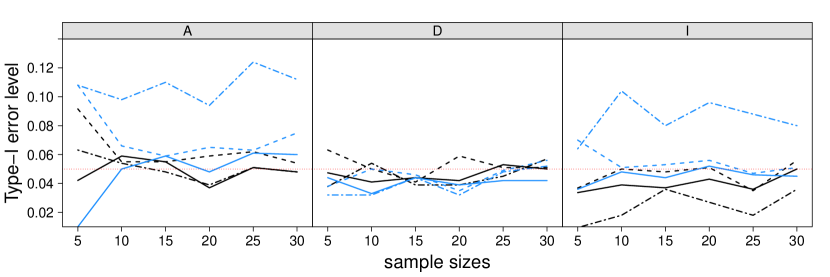
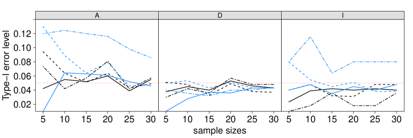
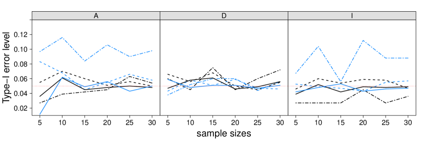
The results for the compound symmetry structure are summarized in Figure 1, Figure 2 visualizes the results for the autoregressive structure and Figure 3 for the Toeplitz structure.
Refer to caption
Figure 1: Type-I𝐼I error rates for Setting 1 (black) and Setting 2 (blue) with a compound symmetry covariance structure for three different tests, namely MCTP (dotted-dashed), bootMCTP (solid) and ATS (dashed).
Refer to caption
Figure 2: Type-I𝐼I error rates for Setting 1 (black) and Setting 2 (blue) with an autoregressive covariance structure for three different tests, namely MCTP (dotted-dashed), bootMCTP (solid) and ATS (dashed).
Refer to caption
Figure 3: Type-I𝐼I error rates for Setting 1 (black) and Setting 2 (blue) with a Toeplitz covariance structure for three different tests, namely MCTP (dotted-dashed), bootMCTP (solid) and ATS (dashed).

The difference between the three different covariance structures is negligible. Even to find the best testing procedure is quite difficult since all three approaches have their advantages and disadvantages. In some cases, the ATS yield better results than the bootstrap version of the MCTP. But note, that the ATS is not an adequate testing procedure for multiple comparisons and therefore, only applicable for global testing problems. Furthermore, the wild bootstrap multiple testing procedure shows pretty good results in controlling the type-I𝐼I errors for rising sample sizes, when compared to the ATS and to the standard MCTP. Especially when comparing the standard and the wild bootstrap based MCTP, there are some cases (“no main effect A𝐴A” and “no interaction effect”) the standard MCTP shows a very liberal behavior, whereas the wild bootstrap MCTP exhibits accurate type-I𝐼I error level control in almost all cases.

4.2 Investigating the impact of different contrast matrices

In this subsection, the novel multiple testing procedures are compared with regard to different contrast matrices. Thus, the ATS is not taken into consideration, because the tests are not comparable in this situation.
Refer to caption
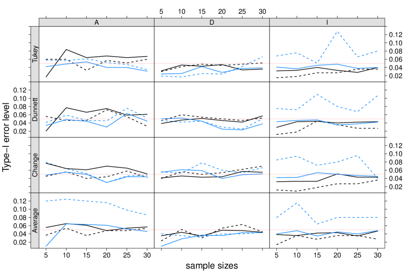
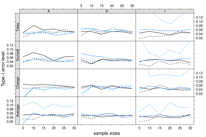
Figure 4: Type-I𝐼I error rates for Setting 1 (black) and Setting 2 (blue) with a compound symmetry covariance structure for four contrast matrices and two tests, namely the MCTP (dashed) and the bootMCTP (solid).
Refer to caption
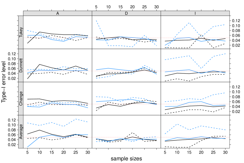
Figure 5: Type-I𝐼I error rates for Setting 1 (black) and Setting 2 (blue) with an autoregressive covariance structure for four contrast matrices and two tests, namely the MCTP (dashed) and the bootMCTP (solid).
Refer to caption
Figure 6: Type-I𝐼I error rates for Setting 1 (black) and Setting 2 (blue) with a Toeplitz covariance structure for four contrast matrices and two tests, namely the MCTP (dashed) and the bootMCTP (solid).

Here, four different contrast matrix are taken into account; namely for all-pairs (Tukey), average, many-to-one (Dunnett) and changepoint comparisons. All corresponding contrast matrices are summarized in Appendix A. Again, two different settings, three different covariance structures, and six different sample sizes are examined. The results are summarized in Figures 4-6 regarding the compound symmetry structure in the first, the autoregressive structure in the second and the Toeplitz structure in the third of this three figures.

Even in case of a comparison between the standard and the wild bootstrap based MCTP, the results between the different covariance structures and the different contrast matrices are quite similar. Some distinctions can be made for the Average-type contrast matrix and the interaction. Regarding the Average-type contrast matrix and the results for no main effect A𝐴A, the standard MCTP shows very liberal behavior in Setting 2. In case of the no interaction effect, the standard MCTP shows a liberal behavior for Setting 2 and tends to conservative results in Setting 1, whereas the wild bootstrap MCTP controls the type-I𝐼I error very accurately.

5 Application to empirical data

Now, the theoretical statements made above are applied to empirical data. First, a dataset included in the R-package nparLD is examined and afterwards data from the Institute of Clinical and Biological Psychology at Ulm University is analyzed.

5.1 Shoulder tip pain study

The following dataset (shoulder) is obtained from the R-package nparLD. The dataset was also studied by Lumley (1996).

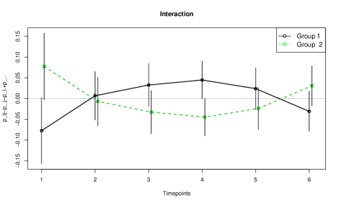
In this study the shoulder pain level of 41 patients after a laparoscopic surgery in the abdomen was examined. During such a surgery, the surgeon fills the abdominal part of the patient with air to have a better view of the body. After this laparoscopic surgery, the air was removed out of the abdomen by using a specific suction procedure. A random subsample of 22 patients (“Y”) was treated with this special suction method. In the other subsample of 19 patients (“N”) the air was left in the abdomen. The patients were asked for their pain score two times a day (morning and evening) for the first three days after the surgery and this score has five different levels from 1 (= low) to 5 (= high). The relative effects of the data for the six different time points are given in Figure 7.

Refer to caption
Figure 7: The relative effects of two different treatment (“Y” and “N”) and six different time points of the shoulder dataset.

In the following, we like to work out the difference between the different groups. Therefore, we apply a Tukey-type contrast matrix to make all-pairs comparisons. Using this results, we like to find out which of the timepoint differ from each other. The results are summarized in Table 1.

Table 1: Many-to-one comparison of the shoulder tip pain study for the standard MCTP in the middle part and for the wild bootstrap MCTP in the right part of the table, significant values are printed in bold.
Comparison p^ip^isubscript^𝑝absent𝑖subscript^𝑝absentsuperscript𝑖\widehat{p}_{\cdot i}-\widehat{p}_{\cdot i^{\prime}} 95%-CI t𝑡t-value p𝑝p-value 95%-CI (wb) p𝑝p-value (wb)
timepoint 2 vs. timepoint 1 0.033 [0.091;0.155]0.0910.155\left[-0.091;\hskip 6.40002pt0.155\right] 0.781 0.963 [0.045;0.111]0.0450.111\left[-0.045;\hskip 6.40002pt0.111\right] 0.443
timepoint 3 vs. timepoint 1 -0.007 [0.124;0.110]0.1240.110\left[-0.124;\hskip 6.40002pt0.110\right] -0.185 0.999 [0.081;0.067]0.0810.067\left[-0.081;\hskip 6.40002pt0.067\right] 0.858
timepoint 4 vs. timepoint 1 0.020 [0.095;0.134]0.0950.134\left[-0.095;\hskip 6.40002pt0.134\right] 0.515 0.994 [0.058;0.098]0.0580.098\left[-0.058;\hskip 6.40002pt0.098\right] 0.624
timepoint 5 vs. timepoint 1 -0.052 [0.171;0.068]0.1710.068\left[-0.171;\hskip 6.40002pt0.068\right] -1.282 0.768 [0.127;0.023]0.1270.023\left[-0.127;\hskip 6.40002pt0.023\right] 0.193
timepoint 6 vs. timepoint 1 -0.077 [0.186;0.035]0.1860.035\left[-0.186;\hskip 6.40002pt0.035\right] -2.028 0.319 [0.145;0.008]0.1450.008\left[-0.145;-0.008\right] 0.035
timepoint 3 vs. timepoint 2 -0.040 [0.111;0.031]0.1110.031\left[-0.111;\hskip 6.40002pt0.031\right] -1.657 0.536 [0.087;0.007]0.0870.007\left[-0.087;\hskip 6.40002pt0.007\right] 0.091
timepoint 4 vs. timepoint 2 -0.013 [0.092;0.067]0.0920.067\left[-0.092;\hskip 6.40002pt0.067\right] -0.469 0.996 [0.064;0.038]0.0640.038\left[-0.064;\hskip 6.40002pt0.038\right] 0.629
timepoint 5 vs. timepoint 2 -0.085 [0.184;0.016]0.1840.016\left[-0.184;\hskip 6.40002pt0.016\right] -2.480 0.141 [0.151;0.018]0.1510.018\left[-0.151;-0.018\right] 0.007
timepoint 6 vs. timepoint 2 -0.109 [0.213;0.003]0.2130.003\left[-0.213;-0.003\right] -3.005 0.045 [0.178;0.038]0.1780.038\left[-0.178;-0.038\right] 0.003
timepoint 4 vs. timepoint 3 0.027 [0.043;0.097]0.0430.097\left[-0.043;\hskip 6.40002pt0.097\right] 1.150 0.838 [0.021;0.075]0.0210.075\left[-0.021;\hskip 6.40002pt0.075\right] 0.253
timepoint 5 vs. timepoint 3 -0.045 [0.139;0.050]0.1390.050\left[-0.139;\hskip 6.40002pt0.050\right] -1.404 0.696 [0.105;0.015]0.1050.015\left[-0.105;\hskip 6.40002pt0.015\right] 0.148
timepoint 6 vs. timepoint 3 -0.069 [0.166;0.029]0.1660.029\left[-0.166;\hskip 6.40002pt0.029\right] -2.075 0.296 [0.133;0.004]0.1330.004\left[-0.133;-0.004\right] 0.031
timepoint 5 vs. timepoint 4 -0.072 [0.149;0.006]0.1490.006\left[-0.149;\hskip 6.40002pt0.006\right] -2.731 0.084 [0.120;0.024]0.1200.024\left[-0.120;-0.024\right] 0.005
timepoint 6 vs. timepoint 4 -0.097 [0.176;0.015]0.1760.015\left[-0.176;-0.015\right] -3.479 0.014 [0.152;0.041]0.1520.041\left[-0.152;-0.041\right] 0.000
timepoint 6 vs. timepoint 5 -0.024 [0.072;0.024]0.0720.024\left[-0.072;\hskip 6.40002pt0.024\right] -1.487 0.644 [0.056;0.008]0.0560.008\left[-0.056;\hskip 6.40002pt0.008\right] 0.145
Y vs. N -0.261 [0.365;0.138]0.3650.138\left[-0.365;-0.138\right] -4.525 <<0.001 [0.365;0.139]0.3650.139\left[-0.365;-0.139\right] <<0.001

First of all, one can see that in almost all cases the CIs of the wild bootstrap MCTP show much shorter widths than the CIs of the standard multiple testing methods. Thus, the wild bootstrap version of the MCTP yields more statistically significant values than the standard version of the MCTP. All of the significant values in the standard MCTP are also significant for the wild bootstrap MCTP. Moreover, the test procedures are consonant and coherent since all p𝑝p-values correspond to the CIs, that is, CIs not including zero lead to a significant p𝑝p-value. With references to the shoulder tip pain study, the standard MCTP yields two pairs of groups, which are statistically different, namely timepoint 2 to timepoint 6 (p=0.045𝑝0.045p=0.045) and timepoint 4 to timepoint 6 (p=0.014𝑝0.014p=0.014). Beyond these two pairs, the wild bootstrap approach detects four other pairs which vary from one to the other group. These are timepoint 1 to timepoint 6 (p=0.035𝑝0.035p=0.035), timepoint 2 to timepoint 5 (p=0.007𝑝0.007p=0.007), timepoint 3 to timepoint 6 (p=0.031𝑝0.031p=0.031) and timepoint 4 to timepoint 5 (p=0.005𝑝0.005p=0.005).

Moreover, an interaction plot for the shoulder tip pain study is given in Figure 8. Generally, in case of a significant interaction effect, one may be interested in the question: “Which profile of which treatment group differs?”.
Refer to caption
Figure 8: Interaction plot for the shoulder tip pain study.

And the courses of such an interaction plot as in Figure 8 may be the first hint. In a second step, pairwise comparisons should be conducted, since only looking at a plot did not verify statistical significance. In case of the shoulder tip pain study, the wild bootstrap version of the MCTP and the ATS yield a significant result (wildMCTP: p=0.013𝑝0.013p=0.013, ATS: p=0.011𝑝0.011p=0.011), whereas the p𝑝p-value of the standard MCTP is 0.055. As one can the in Figure 8, the courses of the two treatment groups are nearly mirrored at the x-axis and thus, are not equal. An all-group comparison, in this case only a comparison between the two treatment groups, yields the following result: The calculated p𝑝p-values for the standard and the wild bootstrap MCTP are <0.001absent0.001<0.001 and thus, this inference procedure confirms the latter assumption.

5.2 Childhood maltreatment study

In this section, a partial dataset of a recent study from the Institute of Clinical and Biological Psychology at Ulm University on childhood maltreatment, postnatal distress and the role of social support is examined. Using the dataset, we like to determine the influence of the childhood maltreatment on the postnatal distress of the mothers. The postnatal distress was measured three times, three (t1subscript𝑡1t_{1}), six (t2subscript𝑡2t_{2}) and nine month (t3subscript𝑡3t_{3}) postpartum. The postnatal psychological distress (dependent variable) was estimated by a combined score of the Perceived Stress Scale (PSS4) and the Hospital Anxiety and Depression Scale (HADS). For the postnatal psychological distress, sum scores of the PSS4 and HADS scales were standardized and added together. The maltreatment experience such as emotional, physical and sexual abuse as well as emotional and physical neglect in the mother’s own childhood was measured with the Childhood Trauma Questionnaire (CTQ). Using quantiles, the CTQ sum score was categorized, resulting in the following value ranges: 25-29 (first quartile), 30-32 (median), 33-37 (third quartile) and 38-103 (maximal value). The relative effects of the data for the three different time points are given in Figure 9.

Refer to caption
Figure 9: The relative effects of women with different CTQ values (categories 1-4) and three different time points.

Figure 9 shows that the estimates of the relative effects of the first three groups are nearly the same. Only the values of the relative effects of the group including the highest CTQ values (group 4) are higher compared to the other groups.

We like to work out the difference between the different CTQ groups and the different measurements. Therefore all-pairs comparisons in both factors are conducted. The results regarding the CTQ categories and the three measurement time points are presented in Table 2.

Table 2: Many-to-one comparison of the childhood maltreatment study for the standard MCTP in the middle part and for the wild bootstrap MCTP in the right part of the table.
Comparison p^ip^isubscript^𝑝absent𝑖subscript^𝑝absentsuperscript𝑖\widehat{p}_{\cdot i}-\widehat{p}_{\cdot i^{\prime}} 95%-CI t𝑡t-value p𝑝p-value 95%-CI (wb) p𝑝p-value (wb)
category 2 vs. category 1 0.023 [0.261;0.303]0.2610.303\left[-0.261;0.303\right] 0.229 0.995 [0.174;0.218]0.1740.218\left[-0.174;0.218\right] 0.821
category 3 vs. category 1 0.023 [0.237;0.280]0.2370.280\left[-0.237;0.280\right] 0.253 0.994 [0.164;0.208]0.1640.208\left[-0.164;0.208\right] 0.804
category 4 vs. category 1 0.138 [0.213;0.455]0.2130.455\left[-0.213;0.455\right] 1.112 0.685 [0.109;0.367]0.1090.367\left[-0.109;0.367\right] 0.271
category 3 vs. category 2 0.000 [0.290;0.291]0.2900.291\left[-0.290;0.291\right] 0.002 1.000 [0.196;0.196]0.1960.196\left[-0.196;0.196\right] 0.997
category 4 vs. category 2 0.115 [0.253;0.453]0.2530.453\left[-0.253;0.453\right] 0.881 0.812 [0.126;0.342]0.1260.342\left[-0.126;0.342\right] 0.400
category 4 vs. category 3 0.114 [0.241;0.442]0.2410.442\left[-0.241;0.442\right] 0.913 0.796 [0.117;0.332]0.1170.332\left[-0.117;0.332\right] 0.360
timepoint 2 vs. timepoint 1 -0.001 [0.109;0.108]0.1090.108\left[-0.109;0.108\right] -0.011 1.000 [0.088;0.086]0.0880.086\left[-0.088;0.086\right] 0.988
timepoint 3 vs. timepoint 1 0.001 [0.108;0.110]0.1080.110\left[-0.108;0.110\right] 0.021 1.000 [0.086;0.088]0.0860.088\left[-0.086;0.088\right] 0.987
timepoint 3 vs. timepoint 2 0.001 [0.021;0.023]0.0210.023\left[-0.021;0.023\right] 0.159 0.985 [0.015;0.017]0.0150.017\left[-0.015;0.017\right] 0.885

Regarding Figure 9, a difference between the time point is not expected since the four presented relative effect courses are nearly straight lines. Nevertheless, a difference of CTQ category 4 (high CTQ values) to all other groups could be expected. However, no significant values – neither in the whole-plot (CTQ category) nor in the sub-plot factor (time) – were calculated. Since the estimated values of the differences of the treatment effects in the time factor are near to zero, all calculated CIs include this value and no significant p𝑝p-value can be computed. But again, in all cases, the CIs regarding the wild bootstrap approach are much shorter than in case of the standard procedure.
Refer to caption
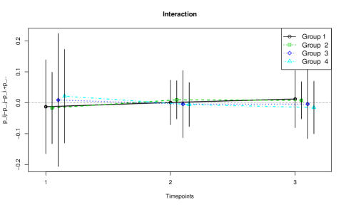
Figure 10: Interaction plot for the childhood maltreatment study.

Additionally, an interaction plot is given in Figure 10. In case of the childhood maltreatment study, the p𝑝p-value for the global null hypothesis of no interaction effect was not significant. The standard MCTP yields a p𝑝p-value of 0.9771, the p𝑝p-value of the ATS was 0.1290, and for the wild bootstrap version of the MCTP, a p𝑝p-value of 0.5856 was computed. All values indicate no different course of the interaction profiles and thus, Figure 10 does, since the profiles are nearly the same.

6 Discussion and Conclusion

Konietschke et al. (2012) already developed multiple, rank-based contrast tests for one-way layouts and also derive SCIs. Additionally, the recent work of Brunner et al. (2018) introduces results for adequate effect measures in repeated measures. Extending both approaches leads to a novel asymptotically exact multiple testing procedure for general factorial split-plot designs. Additionally, the technical details of a wild bootstrap approach for the test statistic were given. Moreover, SCIs for split-plot designs were introduced and also novel SCIs for ratios of different contrast were constructed.

Since the dependence structure within the data becomes much more complex when repeated measures designs are present, classical inference methods to evaluate such data show their limits. Furthermore, the used effect sizes may not be appropriate. Thus, a multiple rank-based testing procedure for split-plot designs and also a wild bootstrap version to obtain asymptotically exact results are studied in this work. The asymptotical exactness of the global testing procedure is an improvement over the classical ATS. Simulation studies show that the novel MCTP controls the type-I𝐼I error level quite accurately. And the applicability of the proposed methods was indicated by the analysis of two different real data examples.

In future works, we like to extend the proposed methods to clustered data, which are often present in clinical studies or other practical applications.

Acknowledgements

The work of Maria Umlauft and Markus Pauly was supported by the German Research Foundation project DFG-PA 2409/3-1.

References

  • (1)
  • Akritas and Arnold (1994) Akritas, M. and Arnold, S. (1994), ‘Fully nonparametric hypotheses for factorial designs I: Multivariate repeated measures designs’, Journal of the American Statistical Association 89(425), 336–343.
  • Akritas and Brunner (1997) Akritas, M. and Brunner, E. (1997), ‘A unified approach to rank tests for mixed models’, Journal of Statistical Planning and Inference 61(2), 249–277.
  • Beyersmann et al. (2013) Beyersmann, J., Di Termini, S. and Pauly, M. (2013), ‘Weak convergence of the wild bootstrap for the Aalen–Johansen estimator of the cumulative incidence function of a competing risk’, Scandinavian Journal of Statistics 40(3), 387–402.
  • Box (1954) Box, G. E. (1954), ‘Some theorems on quadratic forms applied in the study of analysis of variance problems, I. Effect of inequality of variance in the one-way classification’, The Annals of Mathematical Statistics 25(2), 290–302.
  • Bretz et al. (2001) Bretz, F., Genz, A. and Hothorn, L. A. (2001), ‘On the numerical availability of multiple comparison procedures’, Biometrical Journal 43(5), 645–656.
  • Brunner et al. (2018) Brunner, E., Konietschke, F., Pauly, M. and Puri, M. L. (2018), ‘Rank-based procedures in factorial designs: Hypotheses about non-parametric treatment effects’, Journal of the Royal Statistical Society: Series B (Statistical Methodology).
  • Brunner and Munzel (2000) Brunner, E. and Munzel, U. (2000), ‘The nonparametric Behrens-Fisher problem: Asymptotic theory and a small-sample approximation’, Biometrical Journal 42(1), 17–25.
  • Brunner and Placzek (2011) Brunner, E. and Placzek, M. (2011), ‘A Box-type approximation for general two-sample repeated measures – Technical Report’, Abteilung Medizinische Statistik, Georg-August-Universität Göttingen.
  • Dilba et al. (2006) Dilba, G., Bretz, F. and Guiard, V. (2006), ‘Simultaneous confidence sets and confidence intervals for multiple ratios’, Journal of Statistical Planning and Inference 136(8), 2640–2658.
  • Dilba et al. (2004) Dilba, G., Bretz, F., Guiard, V. and Hothorn, L. A. (2004), ‘Simultaneous confidence intervals for ratios with applications to the comparison of several treatments with a control’, Methods Archive 43(5), 465–469.
  • Dobler et al. (2017) Dobler, D., Friedrich, S. and Pauly, M. (2017), ‘Nonparametric MANOVA in Mann-Whitney effects’, Preprint Ulm University.
  • Fieller (1954) Fieller, E. C. (1954), ‘Some problems in interval estimation’, Journal of the Royal Statistical Society: Series B (Statistical Methodology) 16(2), 175–185.
  • Gabriel (1969) Gabriel, K. R. (1969), ‘Simultaneous test procedures – Some theory of multiple comparisons’, The Annals of Mathematical Statistics pp. 224–250.
  • Hasler (2009) Hasler, M. (2009), ‘Extensions of multiple contrast tests’, PhD Thesis, Leibniz-Universität Hannover.
  • Hasler and Hothorn (2008) Hasler, M. and Hothorn, L. A. (2008), ‘Multiple contrast tests in the presence of heteroscedasticity’, Biometrical Journal 50(5), 793–800.
  • Herberich et al. (2010) Herberich, E., Sikorski, J. and Hothorn, T. (2010), ‘A robust procedure for comparing multiple means under heteroscedasticity in unbalanced designs’, PloS one 5(3), e9788.
  • Hochberg and Tamhane (1987) Hochberg, Y. and Tamhane, A. C. (1987), Multiple Comparison Procedures, Wiley, New York.
  • Hothorn et al. (2008) Hothorn, T., Bretz, F. and Westfall, P. (2008), ‘Simultaneous inference in general parametric models’, Biometrical journal 50(3), 346–363.
  • ICH E9 Guideline (1998) ICH E9 Guideline (1998), ‘Statistical principles for clinical trials’, http://www.ich.org/fileadmin/Public_Web_Site/ICH_Products/Guidelines/Efficacy/E9/Step4/E9_Guideline.pdf. [Online; accessed 03-May-2017].
  • Konietschke et al. (2012) Konietschke, F., Hothorn, L. A. and Brunner, E. (2012), ‘Rank-based multiple test procedures and simultaneous confidence intervals’, Electronic Journal of Statistics 6, 738–759.
  • Lumley (1996) Lumley, T. (1996), ‘Generalized estimating equations for ordinal data: A note on working correlation structures’, Biometrics pp. 354–361.
  • Miller (2011) Miller, S. (2011), ‘Simultane Konfidenzintervalle in repeated measures designs’, Diploma Thesis, Georg-August-Universität Göttingen.
  • Mukerjee et al. (1987) Mukerjee, H., Robertson, T. and Wright, F. T. (1987), ‘Comparison of several treatments with a control using multiple contrasts’, Journal of the American Statistical Association 82(399), 902–910.
  • Munzel (2009) Munzel, U. (2009), ‘Nonparametric non-inferiority analyses in the three-arm design with active control and placebo’, Statistics in Medicine 28(29), 3643–3656.
  • Pauly (2011) Pauly, M. (2011), ‘Weighted resampling of martingale difference arrays with applications’, Electronic Journal of Statistics 5, 41–52.
  • Placzek (2013) Placzek, M. (2013), ‘Nichtparametrische simultane Inferenz für faktorielle Repeated Measures Designs’, Master’s Thesis, Georg-August-Universität Göttingen.
  • R Core Team (2015) R Core Team (2015), R: A Language and Environment for Statistical Computing, R Foundation for Statistical Computing, Vienna, Austria.
  • Ruymgaart (1980) Ruymgaart, F. H. (1980), A unified approach to the asymptotic distribution theory of certain midrank statistics, Springer.

Appendix A Contrast Matrices

The Tukey-type contrast matrix is given by

𝐂=(110000101000100001011000010100000011),𝐂matrix110000101000100001011000010100000011\mathbf{C}=\begin{pmatrix}-1&1&0&0&\ldots&0&0\\ -1&0&1&0&\ldots&0&0\\ \vdots&\vdots&\vdots&\vdots&\vdots&\vdots&\vdots\\ -1&0&0&0&\ldots&0&1\\ 0&-1&1&0&\ldots&0&0\\ 0&-1&0&1&\ldots&0&0\\ \vdots&\vdots&\vdots&\vdots&\vdots&\vdots&\vdots\\ 0&0&0&0&\ldots&-1&1\\ \end{pmatrix},

the Dunnett-type contrast matrix by

𝐂=(110000101000100001),𝐂matrix110000101000100001\mathbf{C}=\begin{pmatrix}-1&1&0&0&\ldots&0&0\\ -1&0&1&0&\ldots&0&0\\ \vdots&\vdots&\vdots&\vdots&\vdots&\vdots&\vdots\\ -1&0&0&0&\ldots&0&1\\ \end{pmatrix},

the Average-type contrast matrix by

𝐂=(11a11a11a11a111a11a11a11a11a11),𝐂matrix11𝑎11𝑎11𝑎11𝑎111𝑎11𝑎11𝑎11𝑎11𝑎11\mathbf{C}=\begin{pmatrix}1&-\frac{1}{a-1}&-\frac{1}{a-1}&\ldots&-\frac{1}{a-1}\\ -\frac{1}{a-1}&1&-\frac{1}{a-1}&\ldots&-\frac{1}{a-1}\\ \vdots&\vdots&\ddots&\vdots&\vdots\\ \vdots&\vdots&\vdots&\ddots&\vdots\\ -\frac{1}{a-1}&-\frac{1}{a-1}&-\frac{1}{a-1}&\ldots&1\\ \end{pmatrix},

and finally, the matrix for the changepoint comparisons

𝐂=(1n2i=2anin3i=2anina1i=2aninai=2anin1i=12nin2i=12nin3i=2anina1i=2aninai=2anin1i=1a1nin2i=1a1nin3i=1a1nina1i=1a1ni1).𝐂matrix1subscript𝑛2superscriptsubscript𝑖2𝑎subscript𝑛𝑖subscript𝑛3superscriptsubscript𝑖2𝑎subscript𝑛𝑖subscript𝑛𝑎1superscriptsubscript𝑖2𝑎subscript𝑛𝑖subscript𝑛𝑎superscriptsubscript𝑖2𝑎subscript𝑛𝑖subscript𝑛1superscriptsubscript𝑖12subscript𝑛𝑖subscript𝑛2superscriptsubscript𝑖12subscript𝑛𝑖subscript𝑛3superscriptsubscript𝑖2𝑎subscript𝑛𝑖subscript𝑛𝑎1superscriptsubscript𝑖2𝑎subscript𝑛𝑖subscript𝑛𝑎superscriptsubscript𝑖2𝑎subscript𝑛𝑖subscript𝑛1superscriptsubscript𝑖1𝑎1subscript𝑛𝑖subscript𝑛2superscriptsubscript𝑖1𝑎1subscript𝑛𝑖subscript𝑛3superscriptsubscript𝑖1𝑎1subscript𝑛𝑖subscript𝑛𝑎1superscriptsubscript𝑖1𝑎1subscript𝑛𝑖1\mathbf{C}=\begin{pmatrix}-1&\frac{n_{2}}{\sum_{i=2}^{a}n_{i}}&\frac{n_{3}}{\sum_{i=2}^{a}n_{i}}&\ldots&\frac{n_{a-1}}{\sum_{i=2}^{a}n_{i}}&\frac{n_{a}}{\sum_{i=2}^{a}n_{i}}\\ -\frac{n_{1}}{\sum_{i=1}^{2}n_{i}}&-\frac{n_{2}}{\sum_{i=1}^{2}n_{i}}&\frac{n_{3}}{\sum_{i=2}^{a}n_{i}}&\ldots&\frac{n_{a-1}}{\sum_{i=2}^{a}n_{i}}&\frac{n_{a}}{\sum_{i=2}^{a}n_{i}}\\ \vdots&\vdots&\ddots&\vdots&\vdots&\vdots\\ \vdots&\vdots&\vdots&\ddots&\vdots&\vdots\\ -\frac{n_{1}}{\sum_{i=1}^{a-1}n_{i}}&-\frac{n_{2}}{\sum_{i=1}^{a-1}n_{i}}&-\frac{n_{3}}{\sum_{i=1}^{a-1}n_{i}}&\ldots&-\frac{n_{a-1}}{\sum_{i=1}^{a-1}n_{i}}&1\\ \end{pmatrix}.

The matrices presented in this section are only a small selection of possible contrast matrices. Because of comparability to extisting simulation studies (e.g. see Konietschke et al., 2012) these contrast matrices were chosen for our simulations.

Appendix B Technical Details

B.1 Explicit formulas of the variances and covariances

Here, the sophisticated results of the variance σrs(p,q,p,q)subscript𝜎𝑟𝑠𝑝𝑞superscript𝑝superscript𝑞\sigma_{rs}(p,q,p^{\prime},q^{\prime}) and the covariance σrs,il(p,q,p,q)subscript𝜎𝑟𝑠𝑖𝑙𝑝𝑞superscript𝑝superscript𝑞\sigma_{rs,il}(p,q,p^{\prime},q^{\prime}) defined in Section 2 are given.

Assuming Xijksubscript𝑋𝑖𝑗𝑘X_{ijk} and Xijksubscript𝑋superscript𝑖superscript𝑗superscript𝑘X_{i^{\prime}j^{\prime}k^{\prime}} are independent for ii𝑖superscript𝑖i\neq i^{\prime} or kk𝑘superscript𝑘k\neq k^{\prime}, the entries of the asymptotic covariance matrix are given by

σrs(p,q,p,q)N={τr(s,s)(p,q,p,q),r{p,p},pp,τr(s,s)(p,q,p,q)+τp(q,q)(r,s,r,s),r{p,p},p=p,τr(s,s)(r,q,p,q)τr(q,s)(r,s,p,q),r=p,pp,qs,τr(s,s)(p,q,r,q)τr(s,q)(p,q,r,s),r=p,pp,qs,τr(s,s)(p,q,r,q)τr(s,q)(r,q,r,s)τr(q,s)(r,s,r,q)+τr(q,q)(r,s,r,s),r=p=p,qs,qs,0,else,\displaystyle\begin{split}&\frac{\sigma_{rs}(p,q,p^{\prime},q^{\prime})}{N}\\ &\qquad=\left\{\begin{tabular}[]{p{5.3cm}p{5cm}}$\tau_{r}^{(s,s)}(p,q,p^{\prime},q^{\prime})$,&$r\notin\{p,p^{\prime}\},\;p\neq p^{\prime}$,\\[10.00002pt] $\tau_{r}^{(s,s)}(p,q,p,q^{\prime})+\tau_{p}^{(q,q^{\prime})}(r,s,r,s)$,&$r\notin\{p,p^{\prime}\},\;p=p^{\prime}$,\\[10.00002pt] $\tau_{r}^{(s,s)}(r,q,p^{\prime},q^{\prime})-\tau_{r}^{(q,s)}(r,s,p^{\prime},q^{\prime})$,&$r=p,\;p^{\prime}\neq p^{\prime},\;q\neq s$,\\[10.00002pt] $\tau_{r}^{(s,s)}(p,q,r,q^{\prime})-\tau_{r}^{(s,q^{\prime})}(p,q,r,s)$,&$r=p,\;p^{\prime}\neq p,\;q^{\prime}\neq s$,\\[10.00002pt] $\tau_{r}^{(s,s)}(p,q,r,q^{\prime})-\tau_{r}^{(s,q^{\prime})}(r,q,r,s)-\tau_{r}^{(q,s)}(r,s,r,q^{\prime})+\tau_{r}^{(q,q^{\prime})}(r,s,r,s)$,&$r=p=p^{\prime},\;q\neq s,\;q^{\prime}\neq s$,\\[10.00002pt] $0$,&else,\end{tabular}\right.\end{split} (B.1)

and for (r,s)(i,j)𝑟𝑠𝑖𝑗(r,s)\neq(i,j):

σrs,il(p,q,p,q)N={τr(s,l)(p,q,p,q),r=i,p{i,p},rp,τr(s,q)(p,q,i,l),r=p,p{i,p},ri,τp(q,q)(r,s,i,l),p=i,r{i,p},pp,τp(q,q)(r,s,i,l),p=p,r{i,p},pi,τr(s,l)(p,q,r,q)τr(s,q)(p,q,r,j),r=i=p,p{i,p},ql,τp(q,j)(r,s,p,q)+τp(q,q)(r,s,i,l),p=i=p,r{i,p},ql,τr(s,l)(r,q,p,q)τr(q,l)(r,s,p,q),r=i=p,p{i,p},qs,τr(s,q)(r,q,i,l)+τr(q,q)(r,s,i,l),p=r=p,i{r,p},qs,τr(s,l)(p,q,p,q)+τp(q,q)(r,s,r,j),r=i,p=p,rp,pi,τr(s,q)(p,q,p,l)τp(q,l)(r,s,r,q),r=p,p=i,ri,pp,τr(s,l)(r,q,r,q)τr(s,q)(r,q,r,l)τr(q,l)(r,s,r,q)+τr(q,q)(r,s,r,l),r=p=p=i,sqql,0,else,\displaystyle\begin{split}&\frac{\sigma_{rs,il}(p,q,p^{\prime},q^{\prime})}{N}\\ &\qquad=\left\{\begin{tabular}[]{p{5.3cm}p{5cm}}$\tau_{r}^{(s,l)}(p,q,p^{\prime},q^{\prime})$,&$r=i,\;p\notin\{i,p^{\prime}\},\;r\neq p^{\prime}$,\\[10.00002pt] $-\tau_{r}^{(s,q^{\prime})}(p,q,i,l)$,&$r=p^{\prime},\;p\notin\{i,p^{\prime}\},\;r\neq i$,\\[10.00002pt] $-\tau_{p}^{(q,q^{\prime})}(r,s,i,l)$,&$p=i,\;r\notin\{i,p^{\prime}\},\;p\neq p^{\prime}$,\\[10.00002pt] $\tau_{p}^{(q,q^{\prime})}(r,s,i,l)$,&$p=p^{\prime},\;r\notin\{i,p^{\prime}\},\;p\neq i$,\\[10.00002pt] $\tau_{r}^{(s,l)}(p,q,r,q^{\prime})-\tau_{r}^{(s,q^{\prime})}(p,q,r,j)$,&$r=i=p^{\prime},\;p\notin\{i,p^{\prime}\},\;q^{\prime}\neq l$,\\[10.00002pt] $-\tau_{p}^{(q,j)}(r,s,p,q^{\prime})+\tau_{p}^{(q,q^{\prime})}(r,s,i,l)$,&$p=i=p^{\prime},\;r\notin\{i,p^{\prime}\},\;q^{\prime}\neq l$,\\[10.00002pt] $\tau_{r}^{(s,l)}(r,q,p^{\prime},q^{\prime})-\tau_{r}^{(q,l)}(r,s,p^{\prime},q^{\prime})$,&$r=i=p,\;p^{\prime}\notin\{i,p\},\;q\neq s$,\\[10.00002pt] $-\tau_{r}^{(s,q^{\prime})}(r,q,i,l)+\tau_{r}^{(q,q^{\prime})}(r,s,i,l)$,&$p=r=p^{\prime},\;i\notin\{r,p\},\;q\neq s$,\\[10.00002pt] $\tau_{r}^{(s,l)}(p,q,p,q^{\prime})+\tau_{p}^{(q,q^{\prime})}(r,s,r,j)$,&$r=i,\;p=p^{\prime},\;r\neq p^{\prime},\;p\neq i$,\\[10.00002pt] $-\tau_{r}^{(s,q^{\prime})}(p,q,p,l)-\tau_{p}^{(q,l)}(r,s,r,q^{\prime})$,&$r=p^{\prime},\;p=i,\;r\neq i,\;p\neq p^{\prime}$,\\[10.00002pt] $\tau_{r}^{(s,l)}(r,q,r,q^{\prime})-\tau_{r}^{(s,q^{\prime})}(r,q,r,l)-\tau_{r}^{(q,l)}(r,s,r,q^{\prime})+\tau_{r}^{(q,q^{\prime})}(r,s,r,l)$,&$r=p=p^{\prime}=i,\;s\neq q\neq q^{\prime}\neq l$,\\[10.00002pt] $0$,&else,\end{tabular}\right.\end{split} (B.2)

where

τr(s,j)(p,q,p,q)=1nr𝔼[(Fpq(Xrs1)wpqrs)(Fpq(Xrj1)wpqrj)].superscriptsubscript𝜏𝑟𝑠𝑗𝑝𝑞superscript𝑝superscript𝑞1subscript𝑛𝑟𝔼subscript𝐹𝑝𝑞subscript𝑋𝑟𝑠1subscript𝑤𝑝𝑞𝑟𝑠subscript𝐹superscript𝑝superscript𝑞subscript𝑋𝑟𝑗1subscript𝑤superscript𝑝superscript𝑞𝑟𝑗\tau_{r}^{(s,j)}(p,q,p^{\prime},q^{\prime})=\frac{1}{n_{r}}\operatorname{\mathbb{E}}\left[\left(F_{pq}(X_{rs1})-w_{pqrs}\right)\left(F_{p^{\prime}q^{\prime}}(X_{rj1})-w_{p^{\prime}q^{\prime}rj}\right)\right].

B.2 Confidence intervals for ratios

As already shown in the main part, 𝐓Nratiosuperscriptsubscript𝐓𝑁ratio\mathbf{T}_{N}^{\text{ratio}} is asymptotically multivariate normally distributed with expectation zero and covariance matrix 𝐒=(sm),m=1q𝐒superscriptsubscriptsubscript𝑠𝑚𝑚1𝑞\mathbf{S}=(s_{\ell m})_{\ell,m=1}^{q} with entries sm=(θ𝐝𝐜)𝐕(θm𝐝m𝐜m)(θ𝐝𝐜)𝐕(θ𝐝𝐜)(θm𝐝m𝐜m)𝐕(θm𝐝m𝐜m)subscript𝑠𝑚superscriptsubscript𝜃subscript𝐝subscript𝐜𝐕subscript𝜃𝑚subscript𝐝𝑚subscript𝐜𝑚superscriptsubscript𝜃subscript𝐝subscript𝐜𝐕subscript𝜃subscript𝐝subscript𝐜superscriptsubscript𝜃𝑚subscript𝐝𝑚subscript𝐜𝑚𝐕subscript𝜃𝑚subscript𝐝𝑚subscript𝐜𝑚s_{\ell m}=\frac{(\theta_{\ell}\mathbf{d}_{\ell}-\mathbf{c}_{\ell})^{\prime}\mathbf{V}(\theta_{m}\mathbf{d}_{m}-\mathbf{c}_{m})}{\sqrt{(\theta_{\ell}\mathbf{d}_{\ell}-\mathbf{c}_{\ell})^{\prime}\mathbf{V}(\theta_{\ell}\mathbf{d}_{\ell}-\mathbf{c}_{\ell})}\sqrt{(\theta_{m}\mathbf{d}_{m}-\mathbf{c}_{m})^{\prime}\mathbf{V}(\theta_{m}\mathbf{d}_{m}-\mathbf{c}_{m})}}. One difficulty in the construction of adequate CIs for the ratio θsubscript𝜃\theta_{\ell} is the dependency of the test statistic and the object of estimation. For the easiest case of q=1𝑞1q=1, one only has to deal with a single ratio θ=𝐜𝐩𝐝𝐩𝜃superscript𝐜𝐩superscript𝐝𝐩\theta=\frac{\mathbf{c}^{\prime}\mathbf{p}}{\mathbf{d}^{\prime}\mathbf{p}}. After an application of Fieller’s (1954) theorem, a two-sided CI follows by solving the inequality

|N(θ𝐝𝐜)(𝐩^𝐩)|θ2𝐝𝐕^N𝐝2θ𝐜𝐕^N𝐝+𝐜𝐕^N𝐜c(α),𝑁superscript𝜃𝐝𝐜^𝐩𝐩superscript𝜃2superscript𝐝subscript^𝐕𝑁𝐝2𝜃superscript𝐜subscript^𝐕𝑁𝐝superscript𝐜subscript^𝐕𝑁𝐜𝑐𝛼\frac{|\sqrt{N}\left(\mathbf{\theta}\mathbf{d}-\mathbf{c}\right)^{\prime}\left(\widehat{\mathbf{p}}-\mathbf{p}\right)|}{\mathbf{\theta}^{2}\mathbf{d}^{\prime}\widehat{\mathbf{V}}_{N}\mathbf{d}-2\mathbf{\theta}\mathbf{c}^{\prime}\widehat{\mathbf{V}}_{N}\mathbf{d}+\mathbf{c}^{\prime}\widehat{\mathbf{V}}_{N}\mathbf{c}}\leq c(\alpha), (B.3)

where c(α)𝑐𝛼c(\alpha) is an adequate (1α)1𝛼(1-\alpha) equicoordinate quantile, which depends on τsubscript𝜏\tau_{\ell} through the covariance matrix 𝐒𝐒\mathbf{S}. A way to calculate this corresponding quantile is given at the end of this section. Another representation of inequality (B.3) is given by

Aθ2+Bθ+C0,𝐴superscript𝜃2𝐵𝜃𝐶0A\mathbf{\theta}^{2}+B\mathbf{\theta}+C\leq 0, (B.4)

where

A𝐴\displaystyle A =\displaystyle= (N𝐝𝐩^)2(c(α))2𝐝𝐕^N𝐝,superscript𝑁superscript𝐝^𝐩2superscript𝑐𝛼2superscript𝐝subscript^𝐕𝑁𝐝\displaystyle\left(\sqrt{N}\mathbf{d}^{\prime}\widehat{\mathbf{p}}\right)^{2}-\left(c(\alpha)\right)^{2}\mathbf{d}^{\prime}\widehat{\mathbf{V}}_{N}\mathbf{d},
B𝐵\displaystyle B =\displaystyle= 2[(N𝐜𝐩^)(N𝐝𝐩^)(c(α))2𝐜𝐕^N𝐝] and2delimited-[]𝑁superscript𝐜^𝐩𝑁superscript𝐝^𝐩superscript𝑐𝛼2superscript𝐜subscript^𝐕𝑁𝐝 and\displaystyle-2\left[\left(\sqrt{N}\mathbf{c}^{\prime}\widehat{\mathbf{p}}\right)\left(\sqrt{N}\mathbf{d}^{\prime}\widehat{\mathbf{p}}\right)-\left(c(\alpha)\right)^{2}\mathbf{c}^{\prime}\widehat{\mathbf{V}}_{N}\mathbf{d}\right]\;\text{ and}\;
C𝐶\displaystyle C =\displaystyle= (N𝐜𝐩^)2(c(α))2𝐜𝐕^N𝐜.superscript𝑁superscript𝐜^𝐩2superscript𝑐𝛼2superscript𝐜subscript^𝐕𝑁𝐜\displaystyle\left(\sqrt{N}\mathbf{c}^{\prime}\widehat{\mathbf{p}}\right)^{2}-\left(c(\alpha)\right)^{2}\mathbf{c}^{\prime}\widehat{\mathbf{V}}_{N}\mathbf{c}.

In case of q=1𝑞1q=1, three possible solutions of inequality (B.4) exist. The first one results in the case that all values lie outside the finite interval defined by the two roots of inequalities, the second one results in the entire θ𝜃\theta-axis. The third solution results in a finite interval which is the most desirable solution in this case. This solution corresponds to A>0𝐴0A>0 and thus, B24AC>0superscript𝐵24𝐴𝐶0B^{2}-4AC>0 since the first two solutions only occur with small probability if 𝐝𝐩superscript𝐝𝐩\mathbf{d}^{\prime}\mathbf{p} is significantly from zero. Dilba et al. (2006) gave another representation of A>0𝐴0A>0, namely (c(α))2𝐝𝐕^N𝐝(N𝐝𝐩^)2>1superscript𝑐𝛼2superscript𝐝subscript^𝐕𝑁𝐝superscript𝑁superscript𝐝^𝐩21\frac{(c(\alpha))^{2}\mathbf{d}^{\prime}\widehat{\mathbf{V}}_{N}\mathbf{d}}{\left(\sqrt{N}\mathbf{d}^{\prime}\widehat{\mathbf{p}}\right)^{2}}>1. For the general ratio problem with arbitrary q𝑞q\in\mathbb{N} and in order to guarantee A>0𝐴0A>0 for each component =1,,q1𝑞\ell=1,\ldots,q, say A>0subscript𝐴0A_{\ell}>0, with high probability the following inequalities must be fulfilled

0<y𝐝𝐕^N𝐝N𝐝𝐩^1orN𝐝𝐩^y𝐝𝐕^N𝐝1formulae-sequence0𝑦superscript𝐝subscript^𝐕𝑁𝐝𝑁superscript𝐝^𝐩much-less-than1much-greater-thanor𝑁superscript𝐝^𝐩𝑦superscript𝐝subscript^𝐕𝑁𝐝10<\frac{y\sqrt{\mathbf{d}^{\prime}\widehat{\mathbf{V}}_{N}\mathbf{d}}}{\sqrt{N}\mathbf{d}^{\prime}\widehat{\mathbf{p}}}\ll 1\quad\text{or}\quad\frac{\sqrt{N}\mathbf{d}^{\prime}\widehat{\mathbf{p}}}{y\sqrt{\mathbf{d}^{\prime}\widehat{\mathbf{V}}_{N}\mathbf{d}}}\gg 1 (B.5)

for some relevant point y𝑦y (see Dilba et al., 2006).

To evaluate the right (1α)1𝛼(1-\alpha) equicoordinate quantile for deriving the corresponding SCI, Dilba et al. (2006) introduce three different approaches. Here, we only focus on a resampling approach based on the wild bootstrap introduced in Sections 3.3.1 and 3.3.2. A wild bootstrap based CI can be determined by the following algorithm:

  1. 1.

    For b=1,,B𝑏1𝐵b=1,\ldots,B:

    Calculate the wild bootstrap version Tε,bsuperscriptsubscript𝑇𝜀𝑏T_{\ell}^{\varepsilon,b} of the corresponding test statistic Tsubscript𝑇T_{\ell}.
  2. 2.

    Compute the (1α)1𝛼(1-\alpha) quantile of the values:

    Tmaxε,b=max{|T1ε,b|,,|Tqε,b|}forb=1,,B.formulae-sequencesuperscriptsubscript𝑇max𝜀𝑏superscriptsubscript𝑇1𝜀𝑏superscriptsubscript𝑇𝑞𝜀𝑏for𝑏1𝐵T_{\text{max}}^{\varepsilon,b}=\max\{|T_{1}^{\varepsilon,b}|,\ldots,|T_{q}^{\varepsilon,b}|\}\;\text{for}\;b=1,\ldots,B.

The result of the computation in step 2 leads to the (1α)1𝛼(1-\alpha) equicoordinate wild bootstrap based quantile cε(α)superscript𝑐𝜀𝛼c^{\varepsilon}(\alpha). Finally, combining all the latter results a wild bootstrap based SCI for the ratio θsubscript𝜃\theta_{\ell} can be calculated by

[BB24AC2A,B+B24AC2A],subscript𝐵superscriptsubscript𝐵24subscript𝐴subscript𝐶2subscript𝐴subscript𝐵superscriptsubscript𝐵24subscript𝐴subscript𝐶2subscript𝐴\left[\frac{-B_{\ell}-\sqrt{B_{\ell}^{2}-4A_{\ell}C_{\ell}}}{2A_{\ell}},\frac{-B_{\ell}+\sqrt{B_{\ell}^{2}-4A_{\ell}C_{\ell}}}{2A_{\ell}}\right],

where

Asubscript𝐴\displaystyle A_{\ell} =\displaystyle= (N𝐝𝐩^)2(cε(α))2𝐝𝐕^N𝐝,superscript𝑁subscriptsuperscript𝐝^𝐩2superscriptsuperscript𝑐𝜀𝛼2subscriptsuperscript𝐝subscript^𝐕𝑁subscript𝐝\displaystyle\left(\sqrt{N}\mathbf{d}^{\prime}_{\ell}\widehat{\mathbf{p}}\right)^{2}-\left(c^{\varepsilon}(\alpha)\right)^{2}\mathbf{d}^{\prime}_{\ell}\widehat{\mathbf{V}}_{N}\mathbf{d}_{\ell},
Bsubscript𝐵\displaystyle B_{\ell} =\displaystyle= 2[(N𝐜𝐩^)(N𝐝𝐩^)(cε(α))2𝐜𝐕^N𝐝] and2delimited-[]𝑁subscriptsuperscript𝐜^𝐩𝑁subscriptsuperscript𝐝^𝐩superscriptsuperscript𝑐𝜀𝛼2subscriptsuperscript𝐜subscript^𝐕𝑁subscript𝐝 and\displaystyle-2\left[\left(\sqrt{N}\mathbf{c}^{\prime}_{\ell}\widehat{\mathbf{p}}\right)\left(\sqrt{N}\mathbf{d}^{\prime}_{\ell}\widehat{\mathbf{p}}\right)-\left(c^{\varepsilon}(\alpha)\right)^{2}\mathbf{c}^{\prime}_{\ell}\widehat{\mathbf{V}}_{N}\mathbf{d}_{\ell}\right]\;\text{ and}\;
Csubscript𝐶\displaystyle C_{\ell} =\displaystyle= (N𝐜𝐩^)2(cε(α))2𝐜𝐕^N𝐜.superscript𝑁subscriptsuperscript𝐜^𝐩2superscriptsuperscript𝑐𝜀𝛼2subscriptsuperscript𝐜subscript^𝐕𝑁subscript𝐜\displaystyle\left(\sqrt{N}\mathbf{c}^{\prime}_{\ell}\widehat{\mathbf{p}}\right)^{2}-\left(c^{\varepsilon}(\alpha)\right)^{2}\mathbf{c}^{\prime}_{\ell}\widehat{\mathbf{V}}_{N}\mathbf{c}_{\ell}.

Appendix C The Proofs

Proof of Theorem 3.1

First, note that given the data, only the Rademacher variables εiksubscript𝜀𝑖𝑘\varepsilon_{ik} are random and all other quantities are deterministic. Especially the Dijk(r,s)subscript𝐷𝑖𝑗𝑘𝑟𝑠D_{ijk}(r,s) are deterministic sequences. Second, note that N𝐰^ε𝑁superscript^𝐰𝜀\sqrt{N}\widehat{\mathbf{w}}^{\varepsilon} can be represented as a continuous function of the pooled (i=1,,a)𝑖1𝑎(i=1,\ldots,a) random vectors

N1nik=1niεik(Dijk(r,s))r,s=1a,d,𝑁1subscript𝑛𝑖superscriptsubscript𝑘1subscript𝑛𝑖subscript𝜀𝑖𝑘superscriptsubscriptsubscript𝐷𝑖𝑗𝑘𝑟𝑠𝑟𝑠1𝑎𝑑\sqrt{N}\frac{1}{n_{i}}\sum\limits_{k=1}^{n_{i}}\varepsilon_{ik}\left(D_{ijk}(r,s)\right)_{r,s=1}^{a,d},

which are just sums of row-wise independent random vectors.

The result follows from an application of a multivariate Lindeberg-Feller theorem. Therefore, see Theorem A.1 in Beyersmann et al. (2013) and Theorem 4.1 in Pauly (2011). First, we have to show that the quantity 1Nεik(Dijk(r,s))r,s=1a,d1𝑁subscript𝜀𝑖𝑘superscriptsubscriptsubscript𝐷𝑖𝑗𝑘𝑟𝑠𝑟𝑠1𝑎𝑑\frac{1}{\sqrt{N}}\varepsilon_{ik}(D_{ijk}(r,s))_{r,s=1}^{a,d} fulfilles the multivariate Lindeberg condition given the data. Defining cni=:snic\sqrt{n_{i}}=:s_{n_{i}}, it can be easily shown that

1sni2k=1ni𝔼((εikDijk(r,s))2𝟙{|εikDijk(r,s)|>εsni2})ni0,superscriptsubscript𝑛𝑖1superscriptsubscript𝑠subscript𝑛𝑖2superscriptsubscript𝑘1subscript𝑛𝑖𝔼superscriptsubscript𝜀𝑖𝑘subscript𝐷𝑖𝑗𝑘𝑟𝑠21subscript𝜀𝑖𝑘subscript𝐷𝑖𝑗𝑘𝑟𝑠𝜀superscriptsubscript𝑠subscript𝑛𝑖20\frac{1}{s_{n_{i}}^{2}}\sum_{k=1}^{n_{i}}\operatorname{\mathbb{E}}\left((\varepsilon_{ik}D_{ijk}(r,s))^{2}\mathbbm{1}\{|\varepsilon_{ik}D_{ijk}(r,s)|>\varepsilon s_{n_{i}}^{2}\}\right)\stackrel{{\scriptstyle n_{i}\to\infty}}{{\to}}0,

by an application of the dominated convergence theorem since |εikDijk(r,s)|1subscript𝜀𝑖𝑘subscript𝐷𝑖𝑗𝑘𝑟𝑠1|\varepsilon_{ik}D_{ijk}(r,s)|\leq 1. Furthermore, conditioned on the data the expectation of Nw^pqrsε𝑁superscriptsubscript^𝑤𝑝𝑞𝑟𝑠𝜀\sqrt{N}\hat{w}_{pqrs}^{\varepsilon} is zero. Thus, it remains to show that the conditional covariance between Nw^pqrsε𝑁superscriptsubscript^𝑤𝑝𝑞𝑟𝑠𝜀\sqrt{N}\hat{w}_{pqrs}^{\varepsilon} and Nw^pqijε𝑁superscriptsubscript^𝑤superscript𝑝superscript𝑞𝑖𝑗𝜀\sqrt{N}\hat{w}_{p^{\prime}q^{\prime}ij}^{\varepsilon} converges in probability to the particular element of 𝚺𝚺\bm{\Sigma} for each p,q,r,s,p,q,i,j𝑝𝑞𝑟𝑠superscript𝑝superscript𝑞𝑖𝑗p,q,r,s,p^{\prime},q^{\prime},i,j. First, the calculations regarding

σrs(p,q,p,q)=NCov(Nw^pqrsε,Nw^pqrsε|𝐗)subscript𝜎𝑟𝑠𝑝𝑞superscript𝑝superscript𝑞𝑁Cov𝑁superscriptsubscript^𝑤𝑝𝑞𝑟𝑠𝜀conditional𝑁superscriptsubscript^𝑤superscript𝑝superscript𝑞𝑟𝑠𝜀𝐗\sigma_{rs}(p,q,p^{\prime},q^{\prime})=N\cdot\operatorname{{Cov}}(\sqrt{N}\hat{w}_{pqrs}^{\varepsilon},\sqrt{N}\hat{w}_{p^{\prime}q^{\prime}rs}^{\varepsilon}|\mathbf{X})

are given. For rp,rp,ppformulae-sequence𝑟𝑝formulae-sequence𝑟superscript𝑝𝑝superscript𝑝r\neq p,\;r\neq p^{\prime},\;p\neq p^{\prime} it follows due to independence of the Rademacher variables:

Cov(Nw^pqrsε,Nw^pqrsε|𝐗)Cov𝑁subscriptsuperscript^𝑤𝜀𝑝𝑞𝑟𝑠conditional𝑁subscriptsuperscript^𝑤𝜀superscript𝑝superscript𝑞𝑟𝑠𝐗\displaystyle\operatorname{{Cov}}\left(\sqrt{N}\hat{w}^{\varepsilon}_{pqrs},\sqrt{N}\hat{w}^{\varepsilon}_{p^{\prime}q^{\prime}rs}\big{|}\mathbf{X}\right)
=NCov(1nrk=1nrεrkDrsk(p,q)1npk=1npεpkDpqk(r,s),\displaystyle\qquad=N\cdot\operatorname{{Cov}}\left(\frac{1}{n_{r}}\sum_{k=1}^{n_{r}}\varepsilon_{rk}D_{rsk}(p,q)-\frac{1}{n_{p}}\sum_{k=1}^{n_{p}}\varepsilon_{pk}D_{pqk}(r,s),\right.
1nrk=1nrεrkDrsk(p,q)1npk=1npεpkDpqk(r,s)|𝐗)\displaystyle\qquad\;\;\;\left.\vphantom{\frac{1}{n_{r}}\sum_{k=1}^{n_{r}}}\frac{1}{n_{r}}\sum_{k=1}^{n_{r}}\varepsilon_{rk}D_{rsk}(p^{\prime},q^{\prime})-\frac{1}{n_{p^{\prime}}}\sum_{k=1}^{n_{p^{\prime}}}\varepsilon_{p^{\prime}k}D_{p^{\prime}q^{\prime}k}(r,s)\bigg{|}\mathbf{X}\right)
=NCov(1nrk=1nrεrkDrsk(p,q),1nrk=1nrεrkDrsk(p,q)|𝐗)absent𝑁Cov1subscript𝑛𝑟superscriptsubscript𝑘1subscript𝑛𝑟subscript𝜀𝑟𝑘subscript𝐷𝑟𝑠𝑘𝑝𝑞conditional1subscript𝑛𝑟superscriptsubscript𝑘1subscript𝑛𝑟subscript𝜀𝑟𝑘subscript𝐷𝑟𝑠𝑘superscript𝑝superscript𝑞𝐗\displaystyle\qquad=N\cdot\operatorname{{Cov}}\left(\frac{1}{n_{r}}\sum_{k=1}^{n_{r}}\varepsilon_{rk}D_{rsk}(p,q),\;\frac{1}{n_{r}}\sum_{k=1}^{n_{r}}\varepsilon_{rk}D_{rsk}(p^{\prime},q^{\prime})\bigg{|}\mathbf{X}\right)
=Nnr2k=1nrDrsk(p,q)Drsk(p,q)absent𝑁superscriptsubscript𝑛𝑟2superscriptsubscript𝑘1subscript𝑛𝑟subscript𝐷𝑟𝑠𝑘𝑝𝑞subscript𝐷𝑟𝑠𝑘superscript𝑝superscript𝑞\displaystyle\qquad=\frac{N}{n_{r}^{2}}\sum_{k=1}^{n_{r}}D_{rsk}(p,q)D_{rsk}(p^{\prime},q^{\prime})
pτr(s,s)(p,q,p,q).superscript𝑝absentsuperscriptsubscript𝜏𝑟𝑠𝑠𝑝𝑞superscript𝑝superscript𝑞\displaystyle\qquad\stackrel{{\scriptstyle p}}{{\rightarrow}}\tau_{r}^{(s,s)}(p,q,p^{\prime},q^{\prime}).

For rp,rp,p=pformulae-sequence𝑟𝑝formulae-sequence𝑟superscript𝑝𝑝superscript𝑝r\neq p,\;r\neq p^{\prime},\;p=p^{\prime} we calculate:

Cov(Nw^pqrsε,Nw^pqrsε|𝐗)Cov𝑁subscriptsuperscript^𝑤𝜀𝑝𝑞𝑟𝑠conditional𝑁subscriptsuperscript^𝑤𝜀𝑝superscript𝑞𝑟𝑠𝐗\displaystyle\operatorname{{Cov}}\left(\sqrt{N}\hat{w}^{\varepsilon}_{pqrs},\sqrt{N}\hat{w}^{\varepsilon}_{pq^{\prime}rs}\big{|}\mathbf{X}\right)
=NCov(1nrk=1nrεrkDrsk(p,q)1npk=1npεpkDpqk(r,s),\displaystyle\qquad=N\cdot\operatorname{{Cov}}\left(\frac{1}{n_{r}}\sum_{k=1}^{n_{r}}\varepsilon_{rk}D_{rsk}(p,q)-\frac{1}{n_{p}}\sum_{k=1}^{n_{p}}\varepsilon_{pk}D_{pqk}(r,s),\right.
1nrk=1nrεrkDrsk(p,q)1npk=1npεpkDpqk(r,s)|𝐗)\displaystyle\qquad\;\;\;\left.\vphantom{\frac{1}{n_{r}}\sum_{k=1}^{n_{r}}}\frac{1}{n_{r}}\sum_{k=1}^{n_{r}}\varepsilon_{rk}D_{rsk}(p,q^{\prime})-\frac{1}{n_{p}}\sum_{k=1}^{n_{p}}\varepsilon_{pk}D_{pq^{\prime}k}(r,s)\bigg{|}\mathbf{X}\right)
=NCov(1nrk=1nrεrkDrsk(p,q),1nrk=1nrεrkDrsk(p,q)|𝐗)absent𝑁Cov1subscript𝑛𝑟superscriptsubscript𝑘1subscript𝑛𝑟subscript𝜀𝑟𝑘subscript𝐷𝑟𝑠𝑘𝑝𝑞conditional1subscript𝑛𝑟superscriptsubscript𝑘1subscript𝑛𝑟subscript𝜀𝑟𝑘subscript𝐷𝑟𝑠𝑘𝑝superscript𝑞𝐗\displaystyle\qquad=N\cdot\operatorname{{Cov}}\left(\frac{1}{n_{r}}\sum_{k=1}^{n_{r}}\varepsilon_{rk}D_{rsk}(p,q),\;\frac{1}{n_{r}}\sum_{k=1}^{n_{r}}\varepsilon_{rk}D_{rsk}(p,q^{\prime})\bigg{|}\mathbf{X}\right)
+NCov(1npk=1npεpkDpqk(r,s),1npk=1npεpkDpqk(r,s)|𝐗)𝑁Cov1subscript𝑛𝑝superscriptsubscript𝑘1subscript𝑛𝑝subscript𝜀𝑝𝑘subscript𝐷𝑝𝑞𝑘𝑟𝑠conditional1subscript𝑛𝑝superscriptsubscript𝑘1subscript𝑛𝑝subscript𝜀𝑝𝑘subscript𝐷𝑝superscript𝑞𝑘𝑟𝑠𝐗\displaystyle\qquad\;\;\;+N\cdot\operatorname{{Cov}}\left(-\frac{1}{n_{p}}\sum_{k=1}^{n_{p}}\varepsilon_{pk}D_{pqk}(r,s),\;-\frac{1}{n_{p}}\sum_{k=1}^{n_{p}}\varepsilon_{pk}D_{pq^{\prime}k}(r,s)\bigg{|}\mathbf{X}\right)
=Nnr2k=1nrDrsk(p,q)Drsk(p,q)+Nnp2k=1npDpqk(r,s)Dpqk(r,s)absent𝑁superscriptsubscript𝑛𝑟2superscriptsubscript𝑘1subscript𝑛𝑟subscript𝐷𝑟𝑠𝑘𝑝𝑞subscript𝐷𝑟𝑠𝑘𝑝superscript𝑞𝑁superscriptsubscript𝑛𝑝2superscriptsubscript𝑘1subscript𝑛𝑝subscript𝐷𝑝𝑞𝑘𝑟𝑠subscript𝐷𝑝superscript𝑞𝑘𝑟𝑠\displaystyle\qquad=\frac{N}{n_{r}^{2}}\sum_{k=1}^{n_{r}}D_{rsk}(p,q)D_{rsk}(p,q^{\prime})+\frac{N}{n_{p}^{2}}\sum_{k=1}^{n_{p}}D_{pqk}(r,s)D_{pq^{\prime}k}(r,s)
pτr(s,s)(p,q,p,q)+τp(q,q)(r,s,r,s).superscript𝑝absentsuperscriptsubscript𝜏𝑟𝑠𝑠𝑝𝑞𝑝superscript𝑞superscriptsubscript𝜏𝑝𝑞superscript𝑞𝑟𝑠𝑟𝑠\displaystyle\qquad\stackrel{{\scriptstyle p}}{{\rightarrow}}\tau_{r}^{(s,s)}(p,q,p,q^{\prime})+\tau_{p}^{(q,q^{\prime})}(r,s,r,s).

Similar, for r=p,pp,qsformulae-sequence𝑟𝑝formulae-sequence𝑝superscript𝑝𝑞𝑠r=p,\;p\neq p^{\prime},\;q\neq s, we obtain:

Cov(Nw^rqrsε,Nw^pqrsε|𝐗)Cov𝑁subscriptsuperscript^𝑤𝜀𝑟𝑞𝑟𝑠conditional𝑁subscriptsuperscript^𝑤𝜀superscript𝑝superscript𝑞𝑟𝑠𝐗\displaystyle\operatorname{{Cov}}\left(\sqrt{N}\hat{w}^{\varepsilon}_{rqrs},\sqrt{N}\hat{w}^{\varepsilon}_{p^{\prime}q^{\prime}rs}\big{|}\mathbf{X}\right)
=NCov(1nrk=1nrεrkDrsk(r,q)1nrk=1nrεrkDrqk(r,s),\displaystyle\qquad=N\cdot\operatorname{{Cov}}\left(\frac{1}{n_{r}}\sum_{k=1}^{n_{r}}\varepsilon_{rk}D_{rsk}(r,q)-\frac{1}{n_{r}}\sum_{k=1}^{n_{r}}\varepsilon_{rk}D_{rqk}(r,s),\right.
1nrk=1nrεrkDrsk(p,q)1npk=1npεpkDpqk(r,s)|𝐗)\displaystyle\qquad\;\;\;\left.\vphantom{\frac{1}{n_{r}}\sum_{k=1}^{n_{r}}}\frac{1}{n_{r}}\sum_{k=1}^{n_{r}}\varepsilon_{rk}D_{rsk}(p^{\prime},q^{\prime})-\frac{1}{n_{p^{\prime}}}\sum_{k=1}^{n_{p^{\prime}}}\varepsilon_{p^{\prime}k}D_{p^{\prime}q^{\prime}k}(r,s)\bigg{|}\mathbf{X}\right)
=NCov(1nrk=1nrεrkDrsk(r,q)1nrk=1nrεrkDrqk(r,s),1nrk=1nrεrkDrsk(p,q)|𝐗)absent𝑁𝐶𝑜𝑣1subscript𝑛𝑟superscriptsubscript𝑘1subscript𝑛𝑟subscript𝜀𝑟𝑘subscript𝐷𝑟𝑠𝑘𝑟𝑞1subscript𝑛𝑟superscriptsubscript𝑘1subscript𝑛𝑟subscript𝜀𝑟𝑘subscript𝐷𝑟𝑞𝑘𝑟𝑠conditional1subscript𝑛𝑟superscriptsubscript𝑘1subscript𝑛𝑟subscript𝜀𝑟𝑘subscript𝐷𝑟𝑠𝑘superscript𝑝superscript𝑞𝐗\displaystyle\qquad=N\cdot Cov\left(\frac{1}{n_{r}}\sum_{k=1}^{n_{r}}\varepsilon_{rk}D_{rsk}(r,q)-\frac{1}{n_{r}}\sum_{k=1}^{n_{r}}\varepsilon_{rk}D_{rqk}(r,s),\frac{1}{n_{r}}\sum_{k=1}^{n_{r}}\varepsilon_{rk}D_{rsk}(p^{\prime},q^{\prime})\bigg{|}\mathbf{X}\right)
=NCov(1nrk=1nrεrkDrsk(r,q),1nrk=1nrεrkDrsk(p,q)|𝐗)absent𝑁Cov1subscript𝑛𝑟superscriptsubscript𝑘1subscript𝑛𝑟subscript𝜀𝑟𝑘subscript𝐷𝑟𝑠𝑘𝑟𝑞conditional1subscript𝑛𝑟superscriptsubscript𝑘1subscript𝑛𝑟subscript𝜀𝑟𝑘subscript𝐷𝑟𝑠𝑘superscript𝑝superscript𝑞𝐗\displaystyle\qquad=N\cdot\operatorname{{Cov}}\left(\frac{1}{n_{r}}\sum_{k=1}^{n_{r}}\varepsilon_{rk}D_{rsk}(r,q),\;\frac{1}{n_{r}}\sum_{k=1}^{n_{r}}\varepsilon_{rk}D_{rsk}(p^{\prime},q^{\prime})\bigg{|}\mathbf{X}\right)
+NCov(1nrk=1nrεrkDrqk(r,s),1nrk=1nrεrkDrsk(p,q)|𝐗)𝑁Cov1subscript𝑛𝑟superscriptsubscript𝑘1subscript𝑛𝑟subscript𝜀𝑟𝑘subscript𝐷𝑟𝑞𝑘𝑟𝑠conditional1subscript𝑛𝑟superscriptsubscript𝑘1subscript𝑛𝑟subscript𝜀𝑟𝑘subscript𝐷𝑟𝑠𝑘superscript𝑝superscript𝑞𝐗\displaystyle\qquad\;\;\;+N\cdot\operatorname{{Cov}}\left(-\frac{1}{n_{r}}\sum_{k=1}^{n_{r}}\varepsilon_{rk}D_{rqk}(r,s),\;\frac{1}{n_{r}}\sum_{k=1}^{n_{r}}\varepsilon_{rk}D_{rsk}(p^{\prime},q^{\prime})\bigg{|}\mathbf{X}\right)
=Nnr2k=1nrDrsk(r,q)Drsk(p,q)Nnr2k=1nrDrqk(r,s)Drsk(p,q)absent𝑁superscriptsubscript𝑛𝑟2superscriptsubscript𝑘1subscript𝑛𝑟subscript𝐷𝑟𝑠𝑘𝑟𝑞subscript𝐷𝑟𝑠𝑘superscript𝑝superscript𝑞𝑁superscriptsubscript𝑛𝑟2superscriptsubscript𝑘1subscript𝑛𝑟subscript𝐷𝑟𝑞𝑘𝑟𝑠subscript𝐷𝑟𝑠𝑘superscript𝑝superscript𝑞\displaystyle\qquad=\frac{N}{n_{r}^{2}}\sum_{k=1}^{n_{r}}D_{rsk}(r,q)D_{rsk}(p^{\prime},q^{\prime})-\frac{N}{n_{r}^{2}}\sum_{k=1}^{n_{r}}D_{rqk}(r,s)D_{rsk}(p^{\prime},q^{\prime})
pτr(s,s)(r,q,p,q)τr(q,s)(r,s,p,q),superscript𝑝absentsuperscriptsubscript𝜏𝑟𝑠𝑠𝑟𝑞superscript𝑝superscript𝑞superscriptsubscript𝜏𝑟𝑞𝑠𝑟𝑠superscript𝑝superscript𝑞\displaystyle\qquad\stackrel{{\scriptstyle p}}{{\rightarrow}}\tau_{r}^{(s,s)}(r,q,p^{\prime},q^{\prime})-\tau_{r}^{(q,s)}(r,s,p^{\prime},q^{\prime}),

for r=p,pp,qsformulae-sequence𝑟superscript𝑝formulae-sequence𝑝superscript𝑝superscript𝑞𝑠r=p^{\prime},\;p\neq p^{\prime},\;q^{\prime}\neq s:

Cov(Nw^pqrsε,Nw^rqrsε|𝐗)Cov𝑁subscriptsuperscript^𝑤𝜀𝑝𝑞𝑟𝑠conditional𝑁subscriptsuperscript^𝑤𝜀𝑟superscript𝑞𝑟𝑠𝐗\displaystyle\operatorname{{Cov}}\left(\sqrt{N}\hat{w}^{\varepsilon}_{pqrs},\sqrt{N}\hat{w}^{\varepsilon}_{rq^{\prime}rs}\big{|}\mathbf{X}\right)
=NCov(1nrk=1nrεrkDrsk(p,q)1npk=1npεpkDpqk(r,s),\displaystyle\qquad=N\cdot\operatorname{{Cov}}\left(\frac{1}{n_{r}}\sum_{k=1}^{n_{r}}\varepsilon_{rk}D_{rsk}(p,q)-\frac{1}{n_{p}}\sum_{k=1}^{n_{p}}\varepsilon_{pk}D_{pqk}(r,s),\right.
1nrk=1nrεrkDrsk(r,q)1nrk=1nrεrkDrqk(r,s)|𝐗)\displaystyle\qquad\;\;\;\left.\vphantom{\frac{1}{n_{r}}\sum_{k=1}^{n_{r}}}\frac{1}{n_{r}}\sum_{k=1}^{n_{r}}\varepsilon_{rk}D_{rsk}(r,q^{\prime})-\frac{1}{n_{r}}\sum_{k=1}^{n_{r}}\varepsilon_{rk}D_{rq^{\prime}k}(r,s)\bigg{|}\mathbf{X}\right)
=NCov(1nrk=1nrεrkDrsk(p,q),1nrk=1nrεrkDrsk(r,q)1nrk=1nrεrkDrqk(r,s)|𝐗)absent𝑁𝐶𝑜𝑣1subscript𝑛𝑟superscriptsubscript𝑘1subscript𝑛𝑟subscript𝜀𝑟𝑘subscript𝐷𝑟𝑠𝑘𝑝𝑞1subscript𝑛𝑟superscriptsubscript𝑘1subscript𝑛𝑟subscript𝜀𝑟𝑘subscript𝐷𝑟𝑠𝑘𝑟superscript𝑞conditional1subscript𝑛𝑟superscriptsubscript𝑘1subscript𝑛𝑟subscript𝜀𝑟𝑘subscript𝐷𝑟superscript𝑞𝑘𝑟𝑠𝐗\displaystyle\qquad=N\cdot Cov\left(\frac{1}{n_{r}}\sum_{k=1}^{n_{r}}\varepsilon_{rk}D_{rsk}(p,q),\frac{1}{n_{r}}\sum_{k=1}^{n_{r}}\varepsilon_{rk}D_{rsk}(r,q^{\prime})-\frac{1}{n_{r}}\sum_{k=1}^{n_{r}}\varepsilon_{rk}D_{rq^{\prime}k}(r,s)\bigg{|}\mathbf{X}\right)
=NCov(1nrk=1nrεrkDrsk(p,q),1nrk=1nrεrkDrsk(r,q)|𝐗)absent𝑁Cov1subscript𝑛𝑟superscriptsubscript𝑘1subscript𝑛𝑟subscript𝜀𝑟𝑘subscript𝐷𝑟𝑠𝑘𝑝𝑞conditional1subscript𝑛𝑟superscriptsubscript𝑘1subscript𝑛𝑟subscript𝜀𝑟𝑘subscript𝐷𝑟𝑠𝑘𝑟superscript𝑞𝐗\displaystyle\qquad=N\cdot\operatorname{{Cov}}\left(\frac{1}{n_{r}}\sum_{k=1}^{n_{r}}\varepsilon_{rk}D_{rsk}(p,q),\;\frac{1}{n_{r}}\sum_{k=1}^{n_{r}}\varepsilon_{rk}D_{rsk}(r,q^{\prime})\bigg{|}\mathbf{X}\right)
+NCov(1nrk=1nrεrkDrsk(p,q),1nrk=1nrεrkDrqk(r,s)|𝐗)𝑁Cov1subscript𝑛𝑟superscriptsubscript𝑘1subscript𝑛𝑟subscript𝜀𝑟𝑘subscript𝐷𝑟𝑠𝑘𝑝𝑞conditional1subscript𝑛𝑟superscriptsubscript𝑘1subscript𝑛𝑟subscript𝜀𝑟𝑘subscript𝐷𝑟superscript𝑞𝑘𝑟𝑠𝐗\displaystyle\qquad\;\;\;+N\cdot\operatorname{{Cov}}\left(\frac{1}{n_{r}}\sum_{k=1}^{n_{r}}\varepsilon_{rk}D_{rsk}(p,q),\;-\frac{1}{n_{r}}\sum_{k=1}^{n_{r}}\varepsilon_{rk}D_{rq^{\prime}k}(r,s)\bigg{|}\mathbf{X}\right)
=Nnr2k=1nrDrsk(p,q)Drsk(r,q)Nnr2k=1nrDrsk(p,q)Drqk(r,s)absent𝑁superscriptsubscript𝑛𝑟2superscriptsubscript𝑘1subscript𝑛𝑟subscript𝐷𝑟𝑠𝑘𝑝𝑞subscript𝐷𝑟𝑠𝑘𝑟superscript𝑞𝑁superscriptsubscript𝑛𝑟2superscriptsubscript𝑘1subscript𝑛𝑟subscript𝐷𝑟𝑠𝑘𝑝𝑞subscript𝐷𝑟superscript𝑞𝑘𝑟𝑠\displaystyle\qquad=\frac{N}{n_{r}^{2}}\sum_{k=1}^{n_{r}}D_{rsk}(p,q)D_{rsk}(r,q^{\prime})-\frac{N}{n_{r}^{2}}\sum_{k=1}^{n_{r}}D_{rsk}(p,q)D_{rq^{\prime}k}(r,s)
pτr(s,s)(p,q,r,q)τr(s,q)(p,q,r,s),superscript𝑝absentsuperscriptsubscript𝜏𝑟𝑠𝑠𝑝𝑞𝑟superscript𝑞superscriptsubscript𝜏𝑟𝑠superscript𝑞𝑝𝑞𝑟𝑠\displaystyle\qquad\stackrel{{\scriptstyle p}}{{\rightarrow}}\tau_{r}^{(s,s)}(p,q,r,q^{\prime})-\tau_{r}^{(s,q^{\prime})}(p,q,r,s),

and finally, for r=p,r=p,qs,qsformulae-sequence𝑟𝑝formulae-sequence𝑟superscript𝑝formulae-sequence𝑞𝑠superscript𝑞𝑠r=p,\;r=p^{\prime},\;q\neq s,\;q^{\prime}\neq s:

Cov(Nw^rqrsε,Nw^rqrsε|𝐗)Cov𝑁subscriptsuperscript^𝑤𝜀𝑟𝑞𝑟𝑠conditional𝑁subscriptsuperscript^𝑤𝜀𝑟superscript𝑞𝑟𝑠𝐗\displaystyle\operatorname{{Cov}}\left(\sqrt{N}\hat{w}^{\varepsilon}_{rqrs},\sqrt{N}\hat{w}^{\varepsilon}_{rq^{\prime}rs}\big{|}\mathbf{X}\right)
=NCov(1nrk=1nrεrkDrsk(r,q)1nrk=1nrεrkDrqk(r,s),\displaystyle\qquad=N\cdot\operatorname{{Cov}}\left(\frac{1}{n_{r}}\sum_{k=1}^{n_{r}}\varepsilon_{rk}D_{rsk}(r,q)-\frac{1}{n_{r}}\sum_{k=1}^{n_{r}}\varepsilon_{rk}D_{rqk}(r,s),\right.
1nrk=1nrεrkDrsk(r,q)1nrk=1nrεrkDrqk(r,s)|𝐗)\displaystyle\qquad\;\;\;\left.\vphantom{\frac{1}{n_{r}}\sum_{k=1}^{n_{r}}}\frac{1}{n_{r}}\sum_{k=1}^{n_{r}}\varepsilon_{rk}D_{rsk}(r,q^{\prime})-\frac{1}{n_{r}}\sum_{k=1}^{n_{r}}\varepsilon_{rk}D_{rq^{\prime}k}(r,s)\bigg{|}\mathbf{X}\right)
=NCov(1nrk=1nrεrkDrsk(r,q),1nrk=1nrεrkDrsk(r,q)|𝐗)absent𝑁Cov1subscript𝑛𝑟superscriptsubscript𝑘1subscript𝑛𝑟subscript𝜀𝑟𝑘subscript𝐷𝑟𝑠𝑘𝑟𝑞conditional1subscript𝑛𝑟superscriptsubscript𝑘1subscript𝑛𝑟subscript𝜀𝑟𝑘subscript𝐷𝑟𝑠𝑘𝑟superscript𝑞𝐗\displaystyle\qquad=N\cdot\operatorname{{Cov}}\left(\frac{1}{n_{r}}\sum_{k=1}^{n_{r}}\varepsilon_{rk}D_{rsk}(r,q),\;\frac{1}{n_{r}}\sum_{k=1}^{n_{r}}\varepsilon_{rk}D_{rsk}(r,q^{\prime})\bigg{|}\mathbf{X}\right)
+NCov(1nrk=1nrεrkDrqk(r,s),1nrk=1nrεrkDrsk(r,q)|𝐗)𝑁Cov1subscript𝑛𝑟superscriptsubscript𝑘1subscript𝑛𝑟subscript𝜀𝑟𝑘subscript𝐷𝑟𝑞𝑘𝑟𝑠conditional1subscript𝑛𝑟superscriptsubscript𝑘1subscript𝑛𝑟subscript𝜀𝑟𝑘subscript𝐷𝑟𝑠𝑘𝑟superscript𝑞𝐗\displaystyle\qquad\;\;\;+N\cdot\operatorname{{Cov}}\left(-\frac{1}{n_{r}}\sum_{k=1}^{n_{r}}\varepsilon_{rk}D_{rqk}(r,s),\;\frac{1}{n_{r}}\sum_{k=1}^{n_{r}}\varepsilon_{rk}D_{rsk}(r,q^{\prime})\bigg{|}\mathbf{X}\right)
+NCov(1nrk=1nrεrkDrsk(r,q),1nrk=1nrεrkDrqk(r,s)|𝐗)𝑁Cov1subscript𝑛𝑟superscriptsubscript𝑘1subscript𝑛𝑟subscript𝜀𝑟𝑘subscript𝐷𝑟𝑠𝑘𝑟𝑞conditional1subscript𝑛𝑟superscriptsubscript𝑘1subscript𝑛𝑟subscript𝜀𝑟𝑘subscript𝐷𝑟superscript𝑞𝑘𝑟𝑠𝐗\displaystyle\qquad\;\;\;+N\cdot\operatorname{{Cov}}\left(\frac{1}{n_{r}}\sum_{k=1}^{n_{r}}\varepsilon_{rk}D_{rsk}(r,q),\;-\frac{1}{n_{r}}\sum_{k=1}^{n_{r}}\varepsilon_{rk}D_{rq^{\prime}k}(r,s)\bigg{|}\mathbf{X}\right)
+NCov(1nrk=1nrεrkDrqk(r,s),1nrk=1nrεrkDrqk(r,s)|𝐗)𝑁Cov1subscript𝑛𝑟superscriptsubscript𝑘1subscript𝑛𝑟subscript𝜀𝑟𝑘subscript𝐷𝑟𝑞𝑘𝑟𝑠conditional1subscript𝑛𝑟superscriptsubscript𝑘1subscript𝑛𝑟subscript𝜀𝑟𝑘subscript𝐷𝑟superscript𝑞𝑘𝑟𝑠𝐗\displaystyle\qquad\;\;\;+N\cdot\operatorname{{Cov}}\left(-\frac{1}{n_{r}}\sum_{k=1}^{n_{r}}\varepsilon_{rk}D_{rqk}(r,s),\;-\frac{1}{n_{r}}\sum_{k=1}^{n_{r}}\varepsilon_{rk}D_{rq^{\prime}k}(r,s)\bigg{|}\mathbf{X}\right)
=Nnr2k=1nrDrsk(r,q)Drsk(r,q)Nnr2k=1nrDrqk(r,s)Drsk(r,q)absent𝑁superscriptsubscript𝑛𝑟2superscriptsubscript𝑘1subscript𝑛𝑟subscript𝐷𝑟𝑠𝑘𝑟𝑞subscript𝐷𝑟𝑠𝑘𝑟superscript𝑞𝑁superscriptsubscript𝑛𝑟2superscriptsubscript𝑘1subscript𝑛𝑟subscript𝐷𝑟𝑞𝑘𝑟𝑠subscript𝐷𝑟𝑠𝑘𝑟superscript𝑞\displaystyle\qquad=\frac{N}{n_{r}^{2}}\sum_{k=1}^{n_{r}}D_{rsk}(r,q)D_{rsk}(r,q^{\prime})-\frac{N}{n_{r}^{2}}\sum_{k=1}^{n_{r}}D_{rqk}(r,s)D_{rsk}(r,q^{\prime})
Nnr2k=1nrDrsk(r,q)Drqk(r,s)+Nnr2k=1nrDrqk(r,s)Drqk(r,s)𝑁superscriptsubscript𝑛𝑟2superscriptsubscript𝑘1subscript𝑛𝑟subscript𝐷𝑟𝑠𝑘𝑟𝑞subscript𝐷𝑟superscript𝑞𝑘𝑟𝑠𝑁superscriptsubscript𝑛𝑟2superscriptsubscript𝑘1subscript𝑛𝑟subscript𝐷𝑟𝑞𝑘𝑟𝑠subscript𝐷𝑟superscript𝑞𝑘𝑟𝑠\displaystyle\qquad\;\;\;-\frac{N}{n_{r}^{2}}\sum_{k=1}^{n_{r}}D_{rsk}(r,q)D_{rq^{\prime}k}(r,s)+\frac{N}{n_{r}^{2}}\sum_{k=1}^{n_{r}}D_{rqk}(r,s)D_{rq^{\prime}k}(r,s)
pτr(s,s)(r,q,r,q)τr(q,s)(r,s,r,q)τr(s,q)(r,q,r,s)+τr(q,q)(r,s,r,s).superscript𝑝absentsuperscriptsubscript𝜏𝑟𝑠𝑠𝑟𝑞𝑟superscript𝑞superscriptsubscript𝜏𝑟𝑞𝑠𝑟𝑠𝑟superscript𝑞superscriptsubscript𝜏𝑟𝑠superscript𝑞𝑟𝑞𝑟𝑠superscriptsubscript𝜏𝑟𝑞superscript𝑞𝑟𝑠𝑟𝑠\displaystyle\qquad\stackrel{{\scriptstyle p}}{{\rightarrow}}\tau_{r}^{(s,s)}(r,q,r,q^{\prime})-\tau_{r}^{(q,s)}(r,s,r,q^{\prime})-\tau_{r}^{(s,q^{\prime})}(r,q,r,s)+\tau_{r}^{(q,q^{\prime})}(r,s,r,s).

In all other cases the conditional variance is 0.

Concerning the case of the covariance, where (r,s)(i,j)𝑟𝑠𝑖𝑗(r,s)\neq(i,j), one can proceed in a similar way. Here, only the case r=i,pi,pp,rpformulae-sequence𝑟𝑖formulae-sequence𝑝𝑖formulae-sequence𝑝superscript𝑝𝑟superscript𝑝r=i,\;p\neq i,\;p\neq p^{\prime},\;r\neq p^{\prime} is shown as an example, since the calculation is straightforward as in case of the variance given previously:

Cov(Nw^pqrsε,Nw^pqrjε|𝐗)Cov𝑁subscriptsuperscript^𝑤𝜀𝑝𝑞𝑟𝑠conditional𝑁subscriptsuperscript^𝑤𝜀superscript𝑝superscript𝑞𝑟𝑗𝐗\displaystyle\operatorname{{Cov}}\left(\sqrt{N}\hat{w}^{\varepsilon}_{pqrs},\sqrt{N}\hat{w}^{\varepsilon}_{p^{\prime}q^{\prime}rj}\big{|}\mathbf{X}\right)
=NCov(1nrk=1nrεrkDrsk(p,q)1npk=1npεpkDpqk(r,s),\displaystyle\qquad=N\cdot\operatorname{{Cov}}\left(\frac{1}{n_{r}}\sum_{k=1}^{n_{r}}\varepsilon_{rk}D_{rsk}(p,q)-\frac{1}{n_{p}}\sum_{k=1}^{n_{p}}\varepsilon_{pk}D_{pqk}(r,s),\right.
1nrk=1nrεrkDrjk(p,q)1npk=1npεpkDpqk(r,j)|𝐗)\displaystyle\qquad\;\;\;\left.\vphantom{\frac{1}{n_{r}}\sum_{k=1}^{n_{r}}}\frac{1}{n_{r}}\sum_{k=1}^{n_{r}}\varepsilon_{rk}D_{rjk}(p^{\prime},q^{\prime})-\frac{1}{n_{p}^{\prime}}\sum_{k=1}^{n_{p}^{\prime}}\varepsilon_{p^{\prime}k}D_{p^{\prime}q^{\prime}k}(r,j)\bigg{|}\mathbf{X}\right)
=NCov(1nrk=1nrεrkDrsk(p,q),1nrk=1nrεrkDrjk(p,q)|𝐗)absent𝑁Cov1subscript𝑛𝑟superscriptsubscript𝑘1subscript𝑛𝑟subscript𝜀𝑟𝑘subscript𝐷𝑟𝑠𝑘𝑝𝑞conditional1subscript𝑛𝑟superscriptsubscript𝑘1subscript𝑛𝑟subscript𝜀𝑟𝑘subscript𝐷𝑟𝑗𝑘superscript𝑝superscript𝑞𝐗\displaystyle\qquad=N\cdot\operatorname{{Cov}}\left(\frac{1}{n_{r}}\sum_{k=1}^{n_{r}}\varepsilon_{rk}D_{rsk}(p,q),\;\frac{1}{n_{r}}\sum_{k=1}^{n_{r}}\varepsilon_{rk}D_{rjk}(p^{\prime},q^{\prime})\bigg{|}\mathbf{X}\right)
=Nnr2k=1nrDrsk(p,q)Drjk(p,q)absent𝑁superscriptsubscript𝑛𝑟2superscriptsubscript𝑘1subscript𝑛𝑟subscript𝐷𝑟𝑠𝑘𝑝𝑞subscript𝐷𝑟𝑗𝑘superscript𝑝superscript𝑞\displaystyle\qquad=\frac{N}{n_{r}^{2}}\sum_{k=1}^{n_{r}}D_{rsk}(p,q)D_{rjk}(p^{\prime},q^{\prime})
pτr(s,j)(p,q,p,q).superscript𝑝absentsuperscriptsubscript𝜏𝑟𝑠𝑗𝑝𝑞superscript𝑝superscript𝑞\displaystyle\qquad\stackrel{{\scriptstyle p}}{{\rightarrow}}\tau_{r}^{(s,j)}(p,q,p^{\prime},q^{\prime}).

All other cases can be treated similarly and finally, it follows that the covariance of N𝐰^ε𝑁superscript^𝐰𝜀\sqrt{N}\widehat{\mathbf{w}}^{\varepsilon} conditioned on the data converges in probability to the covariance matrix 𝚺𝚺\bm{\Sigma}. All in all, the distribution of N𝐰^ε𝑁superscript^𝐰𝜀\sqrt{N}\widehat{\mathbf{w}}^{\varepsilon} weakly converges to a multivariate normal distribution with mean zero and covariance matrix 𝚺𝚺\bm{\Sigma} in probability.

And again by the following equation 𝐩^=𝐄ad𝐰^^𝐩subscript𝐄𝑎𝑑^𝐰\widehat{\mathbf{p}}=\mathbf{E}_{ad}\cdot\widehat{\mathbf{w}}, it follows that N𝐩^ε𝑁superscript^𝐩𝜀\sqrt{N}\widehat{\mathbf{p}}^{\varepsilon} is asymptotically multivariate normally distributed with expectation 𝟎0\mathbf{0} and asymptotic covariance matrix 𝐕N=𝐄ad𝚺𝐄adsubscript𝐕𝑁subscript𝐄𝑎𝑑𝚺subscript𝐄𝑎𝑑\mathbf{V}_{N}=\mathbf{E}_{ad}\bm{\Sigma}\mathbf{E}_{ad}. \square

Proof of Corollary 3.2

Using the asymptotic distribution under H0psuperscriptsubscript𝐻0𝑝H_{0}^{p} of FN(𝐌)subscript𝐹𝑁𝐌F_{N}(\mathbf{M}), which is given by

F(𝐌)=i=1aj=1dλij(𝐌𝐕N)tr(𝐌𝐕N)Cij2,𝐹𝐌superscriptsubscript𝑖1𝑎superscriptsubscript𝑗1𝑑subscript𝜆𝑖𝑗subscript𝐌𝐕𝑁trsubscript𝐌𝐕𝑁superscriptsubscript𝐶𝑖𝑗2F(\mathbf{M})=\sum_{i=1}^{a}\sum_{j=1}^{d}\frac{\lambda_{ij}(\mathbf{M}\mathbf{V}_{N})}{\operatorname{tr}(\mathbf{M}\mathbf{V}_{N})}C_{ij}^{2},

where Cijsubscript𝐶𝑖𝑗C_{ij} are independent standard normal random variables and λij(𝐌𝐕)subscript𝜆𝑖𝑗𝐌𝐕\lambda_{ij}(\mathbf{MV}) denote the corresponding eigenvalues of 𝐌𝐕𝐌𝐕\mathbf{MV}, the results follow immediately from Theorem 3.1 by applying the continuous mapping theorem and Slutsky’s theorem:

N𝐩^𝐌𝐩^dAi=1aj=1dλij(𝐌𝐕)ξij,superscript𝑑𝑁superscript^𝐩𝐌^𝐩𝐴similar-tosuperscriptsubscript𝑖1𝑎superscriptsubscript𝑗1𝑑subscript𝜆𝑖𝑗𝐌𝐕subscript𝜉𝑖𝑗N\widehat{\mathbf{p}}^{\prime}\mathbf{M}\widehat{\mathbf{p}}\stackrel{{\scriptstyle d}}{{\to}}A\sim\sum_{i=1}^{a}\sum_{j=1}^{d}\lambda_{ij}(\mathbf{MV})\xi_{ij},

where ξiji.i.dχ12superscriptsimilar-toformulae-sequence𝑖𝑖𝑑subscript𝜉𝑖𝑗subscriptsuperscript𝜒21\xi_{ij}\stackrel{{\scriptstyle i.i.d}}{{\sim}}\chi^{2}_{1} and the multivariate normal distribution of N𝐩^ε𝑁superscript^𝐩𝜀\sqrt{N}\widehat{\mathbf{p}}^{\varepsilon}. \square

Proof of Corollary 3.3

Using definition of a contrast matrix 𝐂=(𝐜1,,𝐜q)𝐂superscriptsubscript𝐜1subscript𝐜𝑞\mathbf{C}=(\mathbf{c}_{1},\ldots,\mathbf{c}_{q})^{\prime}, the proof directly follows by the asymptotic normality of N𝐂𝐩^ε𝑁𝐂superscript^𝐩𝜀\sqrt{N}\mathbf{C}\widehat{\mathbf{p}}^{\varepsilon} and an application of Slutsky’s theorem. \square

Appendix D Power Simulations

In this section, a small power simulation is presented. The simulations are restricted to one covariance structure (compound symmetry) and to a centring matrix 𝐏𝐏\mathbf{P} as a contrast matrix. Again, Setting 1 and Setting 2 as in the main part are simulated and a balanced, homoscedastic design with nij=20subscript𝑛𝑖𝑗20n_{ij}=20 individuals per group is examined. To conduct a power simulation, an effect δ{0,0.1,0.2,,1}𝛿00.10.21\delta\in\{0,0.1,0.2,\ldots,1\} is added to the different factors. Figure 11 summarizes the results for an effect in factor A𝐴A, whereas Figure 12 shows the results for an effect in factor D𝐷D. In case of Setting 1 and an effect in factor A𝐴A, 𝜹=(0,0,0,0,0,0,δ,δ,δ)𝜹superscript000000𝛿𝛿𝛿\bm{\delta}=\left(0,0,0,0,0,0,\delta,\delta,\delta\right)^{\prime} and regarding an effect in factor B𝐵B, the vector is given as follows 𝜹=(0,0,δ,0,0,δ,0,0,δ)𝜹superscript00𝛿00𝛿00𝛿\bm{\delta}=\left(0,0,\delta,0,0,\delta,0,0,\delta\right)^{\prime}. For Settting 2, the 𝜹𝜹\bm{\delta}-vector is constructed in a similar way.
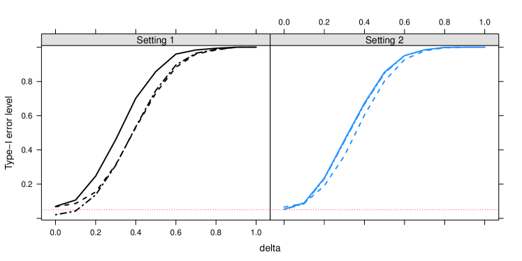
Refer to caption
Figure 11: Power simulation results for Setting 1 (left) and Setting 2 (right) for factor A𝐴A with a compound symmetry covariance structure for three different tests, namely MCTP (dotted-dashed), bootMCTP (solid) and ATS (dashed).

For the power behavior in the first setting and main effect A𝐴A, it can be readily seen from Figure 11 that the bootMCTP has the highest power in case of three repeated measures when compared with the ATS and the standard MCTP. The power functions of the ATS and the standard MCTP are hardly distinguishable. Regarding Setting 2, the power behaviors of both MCTPs are slightly better compared to the ATS.
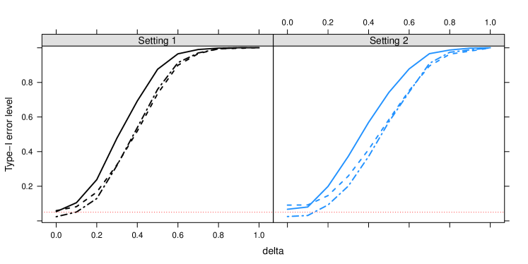
Refer to caption
Figure 12: Power simulation results for Setting 1 (left) and Setting 2 (right) for factor D𝐷D with a compound symmetry covariance structure for three different tests, namely MCTP (dotted-dashed), bootMCTP (solid) and ATS (dashed).

Regarding the results summarized in Figure 12 and Setting 1, the same behavior as given above can be observed. Again, the wild bootstrap version of the MCTP shows the highest power. For small vales of delta the ATS is slightly better than the standard MCTP, but these two power curves become indistinguishable for higher values of delta. The results of Setting 2 are comparable to the results of Setting 1.