Surrounded Vaidya Solution by Cosmological Fields

Abstract

In the present work, we study the general surrounded Vaidya solution by the various cosmological fields and its nature describing the possibility of the formation of naked singularities or black holes. Motivated by the fact that real astrophysical black holes as non-stationary and non-isolated objects are living in non-empty backgrounds, we focus on the black hole subclasses of this general solution describing a dynamical evaporating-accreting black holes in the dynamical cosmological backgrounds of dust, radiation, quintessence, cosmological constant-like and phantom fields, the so called “surrounded Vaidya black hole”. Then, we analyze the timelike geodesics associated with the obtained surrounded black holes and we find that some new correction terms arise relative to the case of Schwarzschild black hole. Also, we address some of the subclasses of the obtained surrounded black hole solution for both dynamical and stationary limits. Moreover, we classify the obtained solutions according to their behaviors under imposing the positive energy condition and discuss how this condition imposes some severe and important restrictions on the black hole and its background field dynamics.

Keywords: Vaidya solution, naked singularity, evaporating-accreting black hole

1 Introduction

Nowadays, we know that black holes are not just a mathematically possible solution to Einstein’s field equations, rather they seem to be some realistic astrophysical objects. It is more than a decade that we have obtained good evidences indicating that most of the galaxies, as our Milky Way, host many stellar active black holes, as well as a super-massive active black hole, in their centers. On the other hand, due to black hole evaporation [3] and accretion-absorbtion processes [1, 2], it is accepted that the mass and other parameters of black holes are not fixed, and should change with time. Therefore, generally speaking, real black holes are non-stationary, and the stationary black holes such as Schwarzschild and Reissner-Nordström are only ideal models. Thus, the study of non-stationary black holes is meaningful and so motivating in the exploration of real black holes. There are a lot of research works on general dynamical black holes and their properties, see the works of Ashtekar $\&$ Krishnan [4] and Hayward [5] as instances. Actually, studying black holes from astrophysical point of view and by astrophysicists has been originated in recent decades due to the dramatic increase in the number of black hole candidates from the sole candidate Cygnus X-1. This study needs a deeper understanding of the black hole physics and especially the black hole radiation by astrophysicists and relativists. Hawking used a quantum field theoretical approach to explore the black hole radiation, for the first time [3]. Afterwards, some models to describe the classical essence of this radiation in a language which is free from the usual quantum field theoretic tools and is more familiar to the astrophysicists and relativists, have been introduced. For instance, the Vaidya solution [6, 7] has provided a simple classical model for the black hole radiation and has been vastly investigated in this regard [8, 9, 10, 11, 12], see also [13, 14, 15, 16, 17, 18, 19, 20, 21, 22, 23, 24] for more studies. In fact, the Vaidya solution is one of the non-static solutions of the Einstein field equations and can be regarded as a generalization of the static Schwarzschild black hole solution. This solution is characterized by a dynamical mass function depending on the retarded time coordinate $u$, i.e $m=m(u)$ and an ingoing/outgoing flow $\sigma(u,r)$. Thus, it can be implemented as a classical model for a dynamical black hole which is effectively evaporating or accreting, regarding its effective flow direction. On the other hand, the Vaidya solution has been used for studying the process of spherical symmetric gravitational collapse and as a testing ground for the cosmic censorship conjecture [25, 26, 27, 28, 29, 30], see also [31] where a possible astrophysical application of the model for describing the energy source of gamma-ray bursts is discussed. These studies also are motivated by the time dependant mass parameter of this solution along with its outgoing radiation flow during the collapse ending by a naked singularity or a black hole. It is shown that if the outgoing flux diverges, the back-reaction will prevent the formation of naked singularity [32]. The observable sign of the formation of a naked singularity, by the collapse process, appears to be the burst of a radiation possessing a non-thermal spectrum, as the Cauchy horizon is approached [33]. Indeed, this is in contrast to the slow evaporation of a black hole via black-body spectrum of the Hawking radiation [3]. Then, it would be important to carefully investigate Vaidya solution to better understanding of real dynamical black holes or the typical signs of naked singularities and to explore if there are any astrophysical objects whose properties resemble those of a naked singularity [33]. The Vaidya solution was generalized to the charged case known as the Bonnor-Vaidya solution [34], see also its application for example in [35, 36, 37, 38, 39]. Also, a generalisation of the Vaidya solution is introduced in [40]. This generalisation is based on the fact that the total supporting energy-momentum tensor of spacetime, constructed from type I and type II energy-momentum tensors [41], is linear in term of the mass function. Consequently, any linear superposition of particular solutions to the Einstein field equations will also a solution. Then, using this approach, we can construct more general solutions such as the Bonnor-Vaidya [34], Vaidya-de Sitter [42], radiating dyon solution [43], Bonnor-Vaidya-de Sitter [44, 45, 46, 47, 48] and the Husain solution [49].

On the other hand, a new exact static solution to Einstein field equations has been recently introduced by Kiselev [50]. Actually, the Kiselev solution is nothing but the static generalization of the Schwarzschild solution to include a non-empty cosmological background, especially well known for the quintessence background. This generalization is well motivated by the fact that black holes in real world are not isolated and are not embedded in empty backgrounds. The black hole solutions coupled to matter fields, such as Kiselev solution, are of interest in studying astrophysical distorted black holes [51, 52, 53, 54], as well as in exploring the ‘no hair’ theorems [55, 56, 57, 58]. Indeed, a crucial assumption for the no-hair theorem is that the black hole is isolated, i.e., the spacetime is asymptotically flat and contains no other sources. However, in real world astrophysical situations this requirement is not fulfilled, for examples, for black holes in binary systems, for black holes surrounded by plasma, or black holes having an accretion disk or jets in their vicinity. All these situations indicate that a black hole may put on different types of wigs. For these cases, the standard no-hair theorem for the isolated black holes can be questioned, see for examples [56, 59]. In a recent research, the authors of [60] discussed on distinguishing rotating Kiselev black hole from naked singularity using spin precession of test gyroscope. In general, since black holes possess strong gravitational attraction such that their nearby matter, even light, cannot escape from their gravitational field, they cannot be observed directly and there are some different ways to detect them in binary systems as well as at the centers of their host galaxies. The most promising way is the accretion process. In the language of astrophysics, the accretion is defined as the inward flow of matter fields surrounding a compact object, such as black holes and neutron stars, due to the gravitational attraction. Then, the process of accretion into black holes is one of the most interesting research fields in relativistic astrophysics [61, 62, 63, 64, 65]. This process may be described by a perfect fluid coupled to general relativity representing a plasma which obeys the equations of ideal or resistive magnetohydrodynamics or a fluid coupled to radiation. Such accretion processes along with their detailed physical descriptions, can be found in [66] and references therein, see also [67, 68, 69, 70, 72, 73, 74, 75]. On the other hand, there are also other kind of accretion processes related to the black holes surrounded by exotic matter fields as potential models of dark energy, whose existence and features are motivated by the problems in the standard model of cosmology. A number of theoretical and observational studies confirmed that our universe in its early stages experienced an inflation process while it is undergoing an accelerated expansion in the late time. In order to explain these events, an energy component, known as the dark energy, is required to be introduced to the framework of general theory of relativity. The cosmological constant is a leading candidate for dark energy while there are other proposals including the dynamical scalar fields such as quintessence and phantom fields. In the Bousso’s work [76], one finds that “Q-space exhibits thermodynamic properties similar to those of the de Sitter horizon. The horizon radius in Q-space grows linearly with time, and consequently the temperature slowly decreases. We find that this behavior is consistent with the first law of thermodynamics: the temperature and entropy respond appropriately to the flux of quintessence stress-energy across the horizon", for a cosmological setup, where “Q-space" stands for quintessence-space. This important result along with the observational data confirming a dark energy fluid responsible for the accelerating expansion of Universe with the equation of state parameter $\omega<-1/3$, has motivated the community to study in detail the black hole solutions in the quintessence background. For some recent studies of Kiselev black holes, see [77] for its generalization to rotating case, [78, 79, 80] for quasinormal modes and Hawking radiation, [81, 82, 83, 84] for thermodynamical studies, [85, 86, 87, 88, 89, 90] for trajectories and particle dynamics around this black hole, [91] for accretion process and [92] for gravitational lensing among the others. One should also note that the Kiselev solution can be implemented for more generic backgrounds of dust, radiation, quintessence, cosmological constant and phantom fields as well as for any realistic combination of these cosmological fields. Then, by the presence of such fields around the black holes, one may have interest to explore some interesting facts such as whether black holes have hair or scalar wigs [93], how black holes affect these cosmological surrounding fields and what are the consequences or what are the influences of these surrounding fields on the features, behaviors and abundance of black holes. In this regard, one may find the reference [94] as a good review including various scenarios of accretion process into black holes, see also [68, 95] for charged black hole accretion. Among the all of the accretion processes, the most interesting one are related to those that the accretion of the surrounding fields enforcing a black hole to shrink. These surrounding field include the scalar fields or fluid violating the weak energy condition, i.e $\rho>0\leavevmode\nobreak\ \&\leavevmode\nobreak\ \rho+p>0$ [94]. Specific scenarios involving the accretion of phantom energy have shown that the black-hole area decreases with the accretion [96, 97, 98, 99]. For example, in [96], it is shown that black holes will gradually vanish as the universe approaches a cosmological big rip state. The big rip scenario for a cosmos occurs when its filling dark energy is the phantom energy with $p<-\rho$. In this scenario, the cosmological phantom field disrupts finally all bounded objects of the universe up to sub-nuclear scales. For the test-field approximation, one may find the accretion process of a scalar field violating the energy conditions leading the decrease in the black holes area in [98, 100]. Moreover, the shrink of the black hole area through the accretion of a phantom scalar field has been confirmed in full nonlinear general relativity [101]. In this regard, the shrink of the black hole area by the accretion of a potentially surrounding field is an interesting phenomena in the sense that it can be an alternative process for black hole evaporation through the Hawking radiation or even be an auxiliary for speeding up it. One physical explanation for a black hole mass diminishing may be is that accreting particles of a phantom scalar field have a total negative energy [102]. Similar particles possessing negative energies are created through the Hawking radiation process and also in the energy extraction process from a black hole by the Penrose mechanism. The effect of phantom-like dark energy onto a charged Reissner-Nordström black hole is studied in [103] and it is found that accretion is possible only through the outer horizon. On the other hand, for scalar fields regarding the energy conditions, there is a possibility indicating that the accretion of a scalar field can be partial such that the amount of accreted scalar field depends on features of the incident wave packet, i.e. the wave number and the width of the packet. This has been studied both in the test-field approximation [104] and in full general relativity [101]. In this line, some studies in the test-field limit indicate that a scalar field can also be sustained by a black hole without being accreted [105].

In the present work, following the approach of [50, 106] introduced for the static black holes, and motivated by the facts that real astrophysical black holes are neither stationary nor isolated and are not embedded in empty backgrounds, we wish to find a more realistic dynamical solution for the classical description of the evaporating-accreting black holes in generic dynamical backgrounds. The organization of the paper is as follows. In section 2, we introduce the general surrounded Vaidya solution, its nature describing the possibility of the formation of naked singularities or black holes, interaction of its possible black holes with their backgrounds as well as its timelike geodesic analysis in the general form. Then, in subsections 3 to 7, we investigate in detail the special classes of this solution as the surrounded Vaidya black hole by the dust, radiation, quintessence, cosmological constant-like and phantom fields, respectively. The paper ends with a conclusion, in section 8.

2 The General Surrounded Vaidya Solutions

In this section, we are looking for the general surrounded Vaidya solutions by the approach of [50, 106]. Then, we consider the general spherical symmetric spacetime metric in the form of

$$ds^{2}=-f(u,r)du^{2}+2\epsilon dudr+r^{2}d\Omega^{2},\leavevmode\nobreak\ \leavevmode\nobreak\ \leavevmode\nobreak\ \epsilon=\pm 1,$$ (1)

where $d\Omega^{2}=d\theta^{2}+sin^{2}\theta d\phi^{2}$ is the two dimensional unit sphere and $f(u,r)$ is a generic metric function depending on both of the advanced/retarded time coordinate $u$ and the radial coordinate $r$. The cases, $\epsilon=-1$ and $\epsilon=+1$ represent the outgoing and ingoing flows corresponding to the effectively evaporating and accreting Vaidya black hole solutions, respectively. Using the metric (1), we obtain nonvanishing components of the Einstein tensor as

$${G^{0}}_{0}={G^{1}}_{1}=\epsilon G_{01}=\epsilon G_{10}=\frac{1}{r^{2}}\left(f^{\prime}r-1+f\right),$$

$${G^{1}}_{0}=\epsilon G_{00}+fG_{01}=-\frac{\dot{f}}{r},$$

$${G^{2}}_{2}=\frac{1}{r^{2}}G_{22}=\frac{1}{r^{2}}\left(rf^{\prime}+\frac{1}{2}r^{2}f^{\prime\prime}\right),$$

$${G^{3}}_{3}=\frac{1}{r^{2}sin^{2}\theta}G_{33}=\frac{1}{r^{2}}\left(rf^{\prime}+\frac{1}{2}r^{2}f^{\prime\prime}\right),$$ (2)

where dot and prime signs represent the derivatives with respect to the time coordinate $u$ and the radial coordinate $r$, respectively. Then, the total energy-momentum supporting this spacetime should have the following non-diagonal form

$${T^{\mu}}_{\nu}=\begin{pmatrix}{T^{0}}_{0}&0&0&0\\ {T^{1}}_{0}&{T^{1}}_{1}&0&0\\ 0&0&{T^{2}}_{2}&0\\ 0&0&0&{T^{3}}_{3}\\ \end{pmatrix},$$ (3)

where also must obey the symmetries in Einstein tensor ${G^{\mu}}_{\nu}$. With respect to the field equations in (2), the equalities ${G^{0}}_{0}={G^{1}}_{1}$ and ${G^{2}}_{2}={G^{3}}_{3}$ require ${T^{0}}_{0}={T^{1}}_{1}$ and ${T^{2}}_{2}={T^{3}}_{3}$, respectively. Then, for the nature of the Vaidya solution in the presence of a dynamical background, one can consider a total energy-momentum tensor supporting the Einstein field equations in the following form

$${T^{\mu}}_{\nu}={\tau^{\mu}}_{\nu}+{\mathcal{T}^{\mu}}_{\nu},$$ (4)

where ${\tau^{\mu}}_{\nu}$ is the energy-momentum tensor associated to the Vaidya null radiation-accretion as

$${\tau^{\mu}}_{\nu}=\sigma k^{\mu}k_{\nu},$$ (5)

such that $\sigma=\sigma(u,r)$ is the measure of the energy flux or the energy density of the outgoing radiation-ingoing accretion flow [107] and $k_{\mu}={\delta^{0}}_{\mu}$ is a null vector field while ${\mathcal{T}^{\mu}}_{\nu}$ is the energy-momentum tensor of the surrounding fluid defined as in [50]

$${\mathcal{T}^{0}}_{0}=-\rho_{s}(u,r),$$

$${\mathcal{T}^{i}}_{j}=-\rho_{s}(u,r)\alpha\left[-(1+3\beta)\frac{r_{i}r^{j}}{r_{n}r^{n}}+\beta{\delta^{i}}_{j}\right],$$ (6)

where subscript $``s"$ stands for the surrounding field which can be a dust, radiation, quintessence, cosmological constant, phantom field or even any complex field constructed by the combination of these fields. This form of energy-momentum for the surrounding fluid is implying that the spatial profile of the Vaidya solution surrounding energy-momentum tensor is proportional to the time component, describing the dynamical energy density $\rho_{s}(u,r)$, with the arbitrary constant parameters $\alpha$ and $\beta$ depending the internal structure of the surrounding fields. The isotropic averaging over the angles results in [50]

$$<{\mathcal{T}^{i}}_{j}>=\frac{\alpha}{3}\rho_{s}(u,r){\delta^{i}}_{j}=p_{s}(u,r){\delta^{i}}_{j},$$ (7)

since we considered $<r^{i}r_{j}>=\frac{1}{3}{\delta^{i}}_{j}r_{n}r^{n}$. Then, we have the barotropic equation of state for the surrounding field as

$$p_{s}(u,r)=\omega_{s}\rho_{s}(u,r),\leavevmode\nobreak\ \leavevmode\nobreak\ \leavevmode\nobreak\ \omega_{s}=\frac{1}{3}\alpha,$$ (8)

where $p_{s}(u,r)$ and $\omega_{s}$ are the dynamical pressure and the constant equation of state parameter of the surrounding field, respectively. Thus, regarding the Einstein tensor components in (2) and the total energy-momentum tensor given by the equations (3)-(2), we have ${\mathcal{T}^{0}}_{0}={\mathcal{T}^{1}}_{1}$ and ${\mathcal{T}^{2}}_{2}={\mathcal{T}^{3}}_{3}$. These exactly provide the so called principle of additivity and linearity considered in [50] in order to determine the free parameter $\beta$ of the energy momentum-tensor ${\mathcal{T}^{\mu}}_{\nu}$ of the surrounding field as

$$\beta=-\frac{1+3\omega_{s}}{6\omega_{s}}.$$ (9)

Then, by substituting $\alpha$ and $\beta$ parameters in (8) and (9) into (2), the non-vanishing components of the surrounding energy-momentum tensor ${\mathcal{T}^{\mu}}_{\nu}$ will be

$${\mathcal{T}^{0}}_{0}={\mathcal{T}^{1}}_{1}=-\rho_{s}(u,r),$$

$${\mathcal{T}^{2}}_{2}={\mathcal{T}^{3}}_{3}=\frac{1}{2}\left(1+3\omega_{s}\right)\rho_{s}(u,r).$$ (10)

Now, by having the Einstein tensor components and the corresponding total energy-momentum tensor ${T^{\mu}}_{\nu}$, one can obtain the associated field equations. Then, the ${G^{0}}_{0}={T^{0}}_{0}$ and ${G^{1}}_{1}={T^{1}}_{1}$ components of the Einstein field equations give the following differential equation

$$\frac{1}{r^{2}}\left(f^{\prime}r-1+f\right)=-\rho_{s}.$$ (11)

Similarly, the ${G^{1}}_{0}={T^{1}}_{0}$ component leads to

$$-\frac{\dot{f}}{r}=\epsilon\sigma,$$ (12)

and ${G^{2}}_{2}={T^{2}}_{2}$ and ${G^{3}}_{3}={T^{3}}_{3}$ components read as

$$\frac{1}{r^{2}}\left(rf^{\prime}+\frac{1}{2}r^{2}f^{\prime\prime}\right)=\frac{1}{2}(1+3\omega_{s})\rho_{s}.$$ (13)

Thus, we see that there are three unknown dynamical functions $f(u,r)$, $\sigma(u,r)$ and $\rho_{s}(u,r)$ which can be determined analytically by the above three differential equations. Simultaneous solving the differential equations (11) and (13), one obtains the following solution for the metric function

$$f(u,r)=1-\frac{2M(u)}{r}-\frac{N_{s}(u)}{{r}^{{3\omega_{s}+1}}},$$ (14)

with the energy density $\rho_{s}(u,r)$ of the surrounding field in the form of

$$\rho_{s}(u,r)=-\frac{3\omega_{s}N_{s}(u)}{{r}^{{3(\omega_{s}+1)}}},$$ (15)

where $M(u)$ and $N_{s}(u)$ are integration coefficients representing the Vaidya dynamical mass and the surrounding dynamical field structure parameter, respectively.

On the other hand, respecting to the weak energy condition imposing the positivity of any kind of energy density of the surrounding field, i.e $\rho_{s}\geq 0$, demands

$$\omega_{s}N_{s}(u)\leq 0.$$ (16)

This implies that for the surrounding field with a positive equation of state parameter $\omega_{s}$, it is needed to have $N_{s}(u)\leq 0$ and conversely for a negative $\omega_{s}$, it is required to have $N_{s}(u)\geq 0$. Then, this condition determines the gravitational nature of the term associated to surrounding field in the metric function $f(u,r)$.

Regarding the metric function (14), the spacetime metric (1) reads as

$$ds^{2}=-\left(1-\frac{2M(u)}{r}-\frac{N_{s}(u)}{{r}^{{3\omega_{s}+1}}}\right)du^{2}+2\epsilon dudr+r^{2}d\Omega^{2},$$ (17)

representing an effectively evaporating-accreting Vaidya spacetime in a dynamical background. One may realize the following distinct subclasses of this general solution as

• The solution by setting $f=f(u,r)$ and $\rho_{s}=\rho_{s}(r)$ in the field equations (11) to (13).

  These considerations lead to $M=M(u)$ and $N_{s}=constant$ in the metric function $f(u,r)$ and $\sigma\neq 0$ for the black hole’s radiation density. In this case, there is no dynamics in the surrounding field and consequently there is no accretion to the black hole. Indeed, this case represents an evaporating black hole solution with $\epsilon=-1$ in a static background. Then, the evaporating black hole in an empty background, i.e $\rho_{s}=0$ [6], and (anti)-de Sitter space, i.e $\rho_{s}=\rho_{\Lambda}=constant$ [42, 108, 109], are special subclasses of our general solution. Some interesting physical features of these solutions can be found in the references [8, 39, 110, 111, 112, 113, 114, 115, 116, 117, 118, 119].

• The solution by setting $f=f(r)$ and $\rho_{s}=\rho_{s}(r)$ in the field equations (11) to (13).

  These considerations lead to $M=constant$, $N_{s}=constant$ in the metric function and $\sigma=0$ for the radiation-accretion density. This case represents a non-dynamical back hole in a static background and consequently, there are no accretion and evaporation. The Schwarzschild black hole as well as its generalization to (anti)-de Sitter background are two special subclasses of our general solution. For a general background, not just the (anti)-de Sitter background, it is interesting that using the following coordinate transformation

  $$du=dt+\frac{\epsilon dr}{1-\frac{2M}{r}-\frac{N_{s}}{{r}^{{3\omega_{s}+1}}}},$$ (18)

  one can obtain the general static solution of the Schwarzschild black hole surrounded by a surrounding field as

  $$ds^{2}=-\left(1-\frac{2M}{r}-\frac{N_{s}}{r^{3\omega_{s}+1}}\right)dt^{2}+\frac{dr^{2}}{1-\frac{2M}{r}-\frac{N_{s}}{r^{3\omega_{s}+1}}}+r^{2}d\Omega^{2},$$ (19)

  which was found by Kiselev [50]. Then, the Kiselev solution also can be obtained as a subclass of our general dynamical solution (17) in the stationary limit.

• The solution for $\epsilon=+1$ with changing the background field parameters as $\omega_{s}\rightarrow\frac{1}{3}(2k-1)$ and $N_{s}(u)\rightarrow-\frac{2g(u)}{2k-1}$.

  By this considerations, we recover the Husain solution describing a null fluid collapse [49] as

  $$ds^{2}=-\left(1-\frac{2M(u)}{r}+\frac{2g(u)}{(2k-1){r}^{{2k}}}\right)du^{2}+2\epsilon dudr+r^{2}d\Omega^{2},$$ (20)

  with the energy density

  $$\rho_{s}(u,r)=\frac{2g(u)}{{r}^{{2k+2}}}.$$ (21)

This solution and it various applications are widely studied in the literature, see for instances [120, 121] and [122, 123] where a barotropic equation of state is considered for the collapse study. There is a difference in the method obtaining the solutions in the present work and in [49] as well as in the other mentioned works. The solution (20), as in [49], is obtained by the “pre-imposed” equation of state $p=k\rho^{a}$, whereas in our approach, the effective equation of state is resulting from the isotropic averaging over the angles for the surrounding field distribution. Our approach is motivated by the present anisotropy in the Einstein tensor components (2) and the corresponding total energy-momentum tensor (3), such that the surrounding fluid behaves effectively as a perfect fluid with the effective (averaged) equation of state $p_{s}(u,r)=\omega_{s}\rho(u,r)$, see (7). As the advantage of this averaging method, one can substitute for $\omega_{s}$ the same known cosmological field equation of state parameters $\frac{1}{3},0,-1,-\frac{2}{3}$ and $-\frac{4}{3}$ for the radiation, dust, cosmological, quintessence and phantom fields, respectively, when the black hole is embedded in these cosmological backgrounds. Substituting the same values of cosmological parameters for $k$, through $p=k\rho^{a}$ even for $a=1$, in (20) gives different solutions with respect to (17) for the general dynamical case as well as for the known static solution in [50] in the stationary limit, by doing a similar transformation to (18). For example, throwing a bunch of dust with the mass of $M_{dust}(=g)$ to the black hole with mass $M$, one expects a resulting metric for the final black hole as $f(r)=1-\frac{2M_{eff}}{r}$ where $M_{eff}=M+M_{dust}$, whereas substituting $k=0$ in the metric (20) gives $f(r)=1-\frac{2M}{r}-2M_{dust}$ which seems to be incorrect due to the gravitational potential form of the final black hole and also the dimensional consideration. One also realizes that, as we will see in the next sections of the paper, there is a possibility of the formation of both the naked singularities and black holes in different backgrounds for the solution with $\epsilon=-1$.

2.1 The Analysis of Naked Singularity or Black Hole Formations

In order to investigate the formation of naked singularity or black hole associated to the obtained solution (17), we follow the approach of [123]. The equation for the radial null geodesics using the metric (1), or (17), can be obtained by setting $ds^{2}=0$ and $d\Omega_{2}^{2}=0$ as

$$\frac{du}{dr}=\frac{2\epsilon}{f(u,r)}.$$ (22)

This system has a singularity at $r=0,\leavevmode\nobreak\ u=0$. Defining the function $X$ as $X=\frac{u}{r}$ gives us the possibility of studying the limiting behavior of $X$ as we approach the singularity located at $r=0,\leavevmode\nobreak\ u=0$, along the radial null geodesics. Denoting this limiting value of $X$ by $X_{0}$, we have

$$\begin{array}[]{c}X_{0}\\ \\ {}\hfil\end{array}\begin{array}[]{c}=lim\leavevmode\nobreak\ \leavevmode\nobreak\ X\\ \tiny u\rightarrow 0\\ \tiny r\rightarrow 0\end{array}\begin{array}[]{c}=lim\leavevmode\nobreak\ \leavevmode\nobreak\ \frac{u}{r}\\ \tiny u\rightarrow 0\\ \tiny r\rightarrow 0\end{array}\begin{array}[]{c}=lim\leavevmode\nobreak\ \leavevmode\nobreak\ \frac{du}{dr}\\ \tiny u\rightarrow 0\\ \tiny r\rightarrow 0\end{array}\begin{array}[]{c}=lim\leavevmode\nobreak\ \leavevmode\nobreak\ \frac{2\epsilon}{f(u,r)}.\\ \tiny u\rightarrow 0\nobreak\leavevmode\nobreak\leavevmode\nobreak\leavevmode\nobreak\leavevmode\\ \tiny r\rightarrow 0\nobreak\leavevmode\nobreak\leavevmode\nobreak\leavevmode\nobreak\leavevmode\end{array}$$ (38)

Using the metric function (14) in (38), we obtain

$$\begin{array}[]{c}\frac{2\epsilon}{X_{0}}=lim\leavevmode\nobreak\ \left(1-\frac{2M(u)}{r}-\frac{N_{s}(u)}{{r}^{{3\omega_{s}+1}}}\right).\\ \tiny u\rightarrow 0\\ \tiny r\rightarrow 0\end{array}$$ (42)

Now, following the method of [123] for our case, we consider $M(u)=mu$ and $N_{s}(u)=nu^{3\omega_{s}+1}$, where $m$ and $n$ are constants. Thus, using (42), we obtain the following algebraic equation in terms of $X_{0}$

$$nX_{0}^{3\omega_{s}+2}+2mX_{0}^{2}-X_{0}+2\epsilon=0.$$ (43)

A black hole will be formed if one obtains only non-positive solutions of this equation. However, if we find a positive real root for (43), then this system describes a naked singularity and consequently provides counterexamples for the cosmic censorship conjecture by Penrose [25]. It is difficult to find exact solutions for $X_{0}$ in (43) for the generic values of $n,m,\epsilon$ and $\omega_{s}$ parameters. However, as a result, one can find that there are possibilities of the formation of both the naked singularities and black holes for the various backgrounds of dust, radiation, quintessence, cosmological constant-like and phantom backgrounds for some particular ranges of $m$ and $n$ parameters. We postpone the detailed study of this equation for the mentioned backgrounds, to the sections 3 to 7.

2.2 The Analysis of the Black Hole-Background Field Interactions

Because in this work, we are mainly interested in the possible interactions between a dynamical black hole and its surrounding background, hence regarding the possibility of formation of black holes as mentioned in the previous subsection and as we will see in the sections 3-7, here we consider only the case that black holes are formed and we analyze in detail the general radiation-accretion profile for the corresponding systems and classify the possible situations under the positive energy condition.

Substituting the metric function (14) in the equation (12) gives the radiation-accretion density of the effectively evaporating-accreting black hole as

$$\sigma(u,r)=\epsilon\left(\frac{2\dot{M}(u)}{r^{2}}+\frac{\dot{N}_{s}(u)}{r^{3\omega_{s}+2}}\right),$$ (44)

where the first and second terms in RHS are the radiation-accretion density corresponding to the mass change of the black hole and the dynamics of the surrounding field, respectively. This shows that for construction of a realistic effectively evaporating-accreting black hole model, one needs to implement such a solution including a dynamical black hole in a dynamical background described by the energy-momentum (2). Considering (44), the following points can be realized.

• By turning off the background field dynamics, i.e. $\dot{N}_{s}(u)=0$, we recover the energy flux associated to the mass change of the central black hole corresponding to the original Vaidya solution [6]. See [107] for more discussion on the properties of the original Vaidya solution.

• For the background field possessing $\omega_{s}>0$, if $\dot{M}(u)$ and $\dot{N}_{s}(u)$ have a same order of magnitude, the surrounding background field contribution to the total density $\sigma(u,r)$ is dominant near the black hole while at far distances from the black hole it decreases faster than the contribution of the black hole mass changing term. In contrast, for the background field possessing $\omega_{s}<0$, the surrounding background field contribution is dominant at large distances while the black hole contribution is dominant near the black hole itself. Then, from the astrophysical point of view, the detected amount of the radiation-accretion density by the observer not only depends on the distance from the black hole but also depends on the nature of background field.

Considering the positive energy density condition (by the weak energy condition) on the total radiation-accretion density $\sigma(u,r)$ in (44) requires

$$\epsilon\left(\frac{2\dot{M}(u)}{r^{2}}+\frac{\dot{N}_{s}(u)}{r^{3\omega_{s}+2}}\right)\geq 0.$$ (45)

This inequality confines the dynamical behaviours of the black hole and its background field at any time and distance $(u,r)$. In the case of a static background, as in the Vaidya’s original solution [6], it is required that $\epsilon$ and $\dot{M}(u)$ have the same signs to have positive energy density. This shows that for a radiating black hole with $\dot{M}(u)<0$ we have $\epsilon=-1$ which represents the outgoing null flow, while for an accreting black hole it is required to have $\epsilon=+1$, representing the ingoing null flow. In the presence of the background dynamics, it is not mandatory that $\epsilon$ and $\dot{M}(u)$ take the same signs and the satisfaction of the positive energy density condition can be achieved even by their opposite signs depending on the background field parameters $\dot{N}_{s}(u)$ and $\omega_{s}$. Based on the relation (45), the dynamical behaviour of the background field is governed by

$$\begin{cases}\dot{N}_{s}(u)\leq-2\,{r}^{3\omega_{s}}\,\dot{M}(u),\leavevmode\nobreak\ \leavevmode\nobreak\ \leavevmode\nobreak\ &\epsilon=-1,\\ \\ \dot{N}_{s}(u)\geq-2\,{r}^{3\omega_{s}}\,\dot{M}(u),&\epsilon=+1.\end{cases}$$ (46)

Then, at any distance $r$ from the black hole, the background field must obey the above conditions. One astrophysical importance of such a physical constraint is that the observer knows the dynamical range of the background field at any distance and that, prior to any observation, he knows how to include or remove the background field contribution if he is only interested in black hole’s contribution, or vice versa. Interestingly, for the special case of $\dot{N}_{s}(u)=-2\,{r}^{3\omega_{s}}\,\dot{M}(u)$, there is no pure radiation-accretion density, i.e $\sigma(u,r)=0$. This case corresponds to two possible physical situations. The first one is related to the situation where for any particular distance $r_{0}$, the background $\dot{N}(u)$ and black hole $\dot{M}(u)$ behave such that their contributions cancel out each others leading to $\sigma(u,r_{0})=0$. The second situation is related to the case that for the given dynamical behaviors of the black hole and its background, one can always find the particular time dependent distance

$$r_{*}(u)=\left(-\frac{\dot{N}_{s}(u)}{2\dot{M}(u)}\right)^{\frac{1}{3\omega_{s}}},$$ (47)

possessing zero energy density $\sigma(u,r_{*}(u))$. For the case of constant rates of $\dot{N}_{s}(u)$ and $\dot{M}(u)$, the distance $r_{*}$ is fixed to a particular value. To have a particular distance at which the density $\sigma(u,r_{*})$ is zero, the positivity of $r_{*}$ also requires that $\dot{M}(u)$ and $\dot{N}_{s}(u)$ have opposite signs. For the cases in which $r_{*}$ is not positive, the lack of a positive real value radial coordinate is interpreted as follows: the radiation-accretion density $\sigma(u,r)$ never and nowhere vanishes.

In the case of being the positive radial coordinate $r_{*}$, for the given radiation-accretion behaviors of the black hole and its surrounding field, i.e $\dot{M}(u)$ and $\dot{N}_{s}(u)$, it is possible to find a distance at which we have no any radiation-accretion energy density contribution. In other words, it turns out that the rate of outgoing radiation energy density of the black hole is exactly balanced by the rate of ingoing absorption rate of surrounding field at the distance $r_{*}$ and vice versa. Beyond or within this particular distance, the various general situations can be realized in the Tables 1 and 2 for the black hole (BH) and its surrounding field (SF). One practical importance of (47) for an astrophysicist is that a particle detector at this distance will detect vanishing radiation-accretion density.

	$\epsilon$	$\omega_{s}$	$\dot{M}$	$\dot{N}$	$r_{*}$	$\sigma({r<r_{*}})$	$\sigma({r=r_{*}})$	$\sigma({r>r_{*}})$	Physical effect
I	-1	+	+	+	-	-	-	-	Not Physical
II	-1	+	-	+	+	-	0	+	Absorbtion of BH’s radiation by SF
III	-1	+	+	-	+	+	0	-	Accretion of SF by BH
IV	-1	+	-	-	-	+	+	+	Accretion/Decay of SF by Evaporating/Vanishing BH
V	-1	-	+	+	-	-	-	-	Not Physical
VI	-1	-	-	+	+	+	0	-	Absorbtion of BH’s radiation by SF
VII	-1	-	+	-	+	-	0	+	Accretion of SF by BH
VIII	-1	-	-	-	-	+	+	+	Accretion/Decay of SF by Evaporating/Vanishing BH

Table 1: General BH and SF parameters for $\epsilon=-1$.

	$\epsilon$	$\omega_{s}$	$\dot{M}$	$\dot{N}$	$r_{*}$	$\sigma({r<r_{*}})$	$\sigma({r=r_{*}})$	$\sigma({r>r_{*}})$	Physical Process
I	+1	+	+	+	-	+	+	+	Accretion of BH and SF
II	+1	+	-	+	+	+	0	-	Absorbtion of BH’s radiation by SF
III	+1	+	+	-	+	-	0	+	Accretion of SF by BH
IV	+1	+	-	-	-	-	-	-	Not Physical
V	+1	-	+	+	-	+	+	+	Accretion of BH and SF
VI	+1	-	-	+	+	-	0	+	Absorbtion of BH’s radiation by SF
VII	+1	-	+	-	+	+	0	-	Accretion of SF by BH
VIII	+1	-	-	-	-	-	-	-	Not Physical

Table 2: General BH and SF parameters for $\epsilon=+1$.

Then, regarding these tables and Eq.(45), we find the following results.

• The cases possessing negative values of $r_{*}$ (the cases I, IV, V and VIII) mean that the radiation-accretion density does not vanish somewhere and forever. Among these cases, the ones which have positive $\sigma(u,r)$ are only physical, i.e the cases IV and VIII for $\epsilon=-1$, and I and V for $\epsilon=+1$. Then, one realizes that how the weak energy condition causes in practice the nonphysical events to be hidden to an astrophysicist aiming to investigate a black hole and his surrounding field.

• The remaining positive values of $r_{*}$, corresponding to a zero radiation-accretion density, are physically viable and their corresponding physical processes are listed in the last column. These properties are determined according to the behaviours of the parameters $\epsilon$, $\omega_{s}$, and quantities $\dot{M}(u)$, $\dot{N}_{s}(u)$, and $\sigma(u,r)$. Those values of $r_{*}$ corresponding to the negative energy density $\sigma(u,r)$ represent no physical situation about the evaporation-absorption or accretion. The real features of those regions are hidden by the weak energy condition. Then, it is physically reasonable to do any astrophysical experiment in the regions respecting the energy condition.

• For $\omega_{s}>-\frac{2}{3}$, the particular distance $r_{*}$, where $\sigma(u,r)$ vanishes, corresponds to two possible cases as $r_{*}(u)=\left(-\frac{\dot{N}_{s}(u)}{2\dot{M}(u)}\right)^{\frac{1}{3\omega_{s}}}$ and $r_{*}=\infty$. In the first case, for $-\frac{2}{3}<\omega_{s}<0$ with $|\dot{N}_{s}(u)|\ll|\dot{M}(u)|$ and for $\omega_{s}\geq 0$ with $|\dot{M}(u)|\ll|\dot{N}_{s}(u)|$, we have $r_{*}\rightarrow\infty$. This means that the first situation indicates that black hole evolves very faster than its background while the second indicates that black hole evolves very slow relative to its background. By satisfaction of these dynamical conditions to hold $r_{*}\rightarrow\infty$, the positive energy density is respected everywhere in the spacetime. Then, in practice, an astrophysical observer can detect a radiation-accretion density resulting from the interaction of the black hole with its surrounding field even at far distances, in which for $-\frac{2}{3}<\omega_{s}<0$ and $\omega_{s}\geq 0$ the main contribution in the detected radiation-accretion density belongs to the black hole and surrounding field, respectively. In other cases, the positive energy density will be respected in some regions while violated beyond those regions.

• For $\omega_{s}\leq-\frac{2}{3}$, the particular distance $r_{*}$ is given as $r_{*}(u)=\left(-\frac{\dot{N}_{s}(u)}{2\dot{M}(u)}\right)^{\frac{1}{3\omega_{s}}}$. Then, for a rapidly evolving black hole relative to its background, i.e $|\dot{N}_{s}(u)|\ll|\dot{M}(u)|$, we have $r_{*}\rightarrow\infty$. This case implies an evolving black hole in an almost static background in which the positive energy condition is respected everywhere in this spacetime. Then, for $\omega_{s}\leq-\frac{2}{3}$ representing a dark energy fluid, an astrophysicist finds that it is the black hole which has the main contribution in the radiation-accretion density.

2.3 Timelike Geodesics for the Surrounded Black Holes

The geodesics for our metric (1), or (17), will all lie on a plane due to the spherical symmetry in which for the sake of simplicity, one can choose $\theta=\pi/2$. The geodesic equations for the above spacetime metric can be derived by varying the following action

$$I=\int\mathcal{L}d\tau=\frac{1}{2}\int\left(-f(u,r)\overset{*}{u}^{2}+2\epsilon\overset{*}{u}\overset{*}{r}+r^{2}\overset{*}{\varphi}^{2}\right)d\tau,$$ (48)

where the star sign denotes the derivative with respect to the proper time $\tau$. Then, we have the following three equations

$$\overset{*}{\varphi}=\frac{L}{r^{2}},$$ (49)

and

$$-\frac{1}{2}f^{\prime}\overset{*}{u}^{2}+r\overset{*}{\varphi}^{2}-\epsilon\overset{**}{u}=0,$$ (50)

and

$$\epsilon\overset{**}{r}=\frac{1}{2}\dot{f}\overset{*}{u}^{2}+f\overset{**}{u}+f^{\prime}\overset{*}{u}\overset{*}{r},$$ (51)

for $\varphi,r$ and $u$ variables respectively, where $L$ is the conserved angular momentum per unit mass and dot and prime signs denote the derivative with respect to $u$ and $r$, respectively. Using (49) in (50), one finds

$$f\overset{**}{u}=\epsilon f\frac{L^{2}}{r^{3}}-\frac{1}{2}\epsilon ff^{\prime}\overset{*}{u}^{2}.$$ (52)

On the other, using the timelike geodesics condition as $g_{\mu\nu}\dot{x}^{\mu}\dot{x}^{\nu}=-1$, one finds

$$f^{\prime}\overset{*}{r}\overset{*}{u}=-\frac{1}{2}\epsilon f^{\prime}+\frac{1}{2}\epsilon ff^{\prime}-\frac{1}{2}\epsilon f^{\prime}\frac{L^{2}}{r^{2}}\overset{*}{u}^{2},$$ (53)

where the equation (49) has been used. Then, by substituting (52) and (53) in (51), we arrive at the following general equation of motion in term of the metric function for the radial coordinate

$$\overset{**}{r}=\frac{1}{2}\epsilon\dot{f}\overset{*}{u}^{2}-\frac{1}{2}f^{\prime}-\frac{1}{2}f^{\prime}\frac{L^{2}}{r^{2}}+f\frac{L^{2}}{r^{3}}.$$ (54)

Then, using the metric function $f(u,r)=1-\frac{2M(u)}{r}-\frac{N_{s}(u)}{{r}^{{3\omega_{s}+1}}}$, this equation takes the following form

$$\overset{**}{r} = -\frac{M(u)}{r^{2}}+\frac{L^{2}}{r^{3}}-\frac{3M(u)L^{2}}{r^{4}}$$ (55)

$$-\frac{(3\omega_{s}+1)N(u)}{2r^{3\omega_{s}+2}}-\frac{3(\omega_{s}+1)N(u)L^{2}}{2r^{3\omega_{s}+4}}$$

$$+\frac{1}{2}\epsilon\dot{f}\overset{*}{u}^{2}.$$

Then, one realizes the following three interesting points.

1. The terms in the first line are exactly the same as that of the standard Schwarzschild black hole in which the first term represents the Newtonian gravitational force, the second term represents a repulsive centrifugal force and the third term is the relativistic correction of the Einstein GR which accounts for the perihelion precession.

2. The terms in the second line are new correction terms due to the presence of the background field which surrounds the Vaidya black hole, in which its first term is similar to the term of gravitational potential in the first line, while its second term is similar to the relativistic correction of GR. Then, regarding (55) one realizes that for the more realistic non-empty backgrounds, the geodesic equation of any object depends strictly not only on the mass of the central object of the system and the conserved angular momentum of the orbiting body, but also on the background field nature. The new correction terms may be small in general in comparison to their Schwarzschild counterparts (the first and third terms in the first line). However, one can show that there are possibilities that these terms are comparable to them. Then, in order to find a situation where these forces are comparable to the Newtonian gravitational force and the GR correction term in (55), we define the distances $D_{s_{1}}$ and $D_{s_{2}}$ which satisfy $|\frac{a_{s_{1}}}{a_{N}}|\simeq 1$ and $|\frac{a_{s_{2}}}{a_{L}}|\simeq 1$, respectively, where $a_{N}$, $a_{L}$ are the Newtonian and the relativistic correction accelerations, respectively, and $a_{s_{1}}$ and $a_{s_{2}}$ are defined as

   $$a_{s_{1}}=\frac{(3\omega_{s}+1)N(u)}{2r^{3\omega_{s}+2}},\leavevmode\nobreak\ \leavevmode\nobreak\ \leavevmode\nobreak\ \leavevmode\nobreak\ \leavevmode\nobreak\ a_{s_{2}}=\frac{3(\omega_{s}+1)N(u)L^{2}}{2r^{3\omega_{s}+4}}.$$ (56)

   Then, the distances $D_{s_{1}}$ and $D_{s_{2}}$ will be given by

   $$D_{s_{1}}^{3\omega_{s}}=\left(\frac{|(3\omega_{s}+1)N_{s}(u)|}{2M(u)}\right),\leavevmode\nobreak\ \leavevmode\nobreak\ \leavevmode\nobreak\ \leavevmode\nobreak\ \leavevmode\nobreak\ D_{s_{2}}^{3\omega_{s}}=\left(\frac{|(\omega_{s}+1)N_{s}(u)|}{2M(u)}\right).$$ (57)

   We give the detailed study of these particular distances for the various cosmological backgrounds, in the sections 3 to 7.

3. The new correction term in the third line is also a non-Newtonian gravitational force originated from the dynamics of black hole and its surrounding field. It is associated with the radiation-accretion power of the black hole and its surrounding field. Calling this acceleration as the induced acceleration $a_{i}$, where the subscript $i$ stands for “induced”, we have

   $$a_{i}=\frac{1}{2}\epsilon\dot{f}\overset{*}{u}^{2}=-\epsilon\left(\frac{\dot{M}(u)}{r}+\frac{\dot{N}(u)}{2r^{3\omega_{s}+1}}\right)\overset{*}{u}^{2},$$ (58)

   in which, following Lindquist, Schwartz and Misner [124], one can define the generalized “total apparent flux” as $\mathcal{A}_{F}=\epsilon\left(\dot{M}(u)+\frac{\dot{N}(u)}{2r^{3\omega_{s}}}\right){\overset{*}{u}}^{2}=\mathfrak{L}+\frac{\mathfrak{N}}{2r^{3\omega_{s}}}$ where $\mathfrak{L}$ and $\mathfrak{N}$ are the apparent fluxes associated to the black hole and its surrounding field radiation-accretion rates, respectively. Using these definitions, (58) takes the following form

   $$a_{i}=-\frac{\mathfrak{L}}{r}-\frac{\mathfrak{N}}{2r^{3\omega_{s}+1}}.$$ (59)

   As mentioned in [124], this new correction term may be small in general in comparison to the Newtonian term. However, one can show that there are possibilities that these two terms are comparable. Then, in order to find a situation where this induced force is comparable to the Newtonian gravitational force in (55), we define the distance $R$ which satisfies $a_{i}\simeq a_{N}$, where $a_{N}$ is the Newtonian gravitational acceleration. Then, this distance will be given by the solutions of the following equation for different values of $M$, $\omega_{s}$ and apparent fluxes $\mathfrak{L}$ and $\mathfrak{N}$ as

   $$\mathfrak{L}R^{3\omega_{s}}+\frac{1}{2}\mathfrak{N}\simeq MR^{3\omega_{s}-1}.$$ (60)

   Finding the general solutions to this equation in terms of the generic $\mathfrak{L},\mathfrak{N},M$ and $\omega_{s}$ parameters is not simple. However, one can find that there are possible solutions for the various backgrounds of dust, radiation, quintessence, cosmological constant-like and phantom fields for some particular ranges of the parameters. We give the detailed study of this equation for the mentioned backgrounds, in the sections 3 to 7.

3 Evaporating-Accreting Vaidya Black Hole Surrounded by the Dust Field

3.1 Naked Singularity or Black Hole Formation Analysis

For this case, the equation (43) takes the following form

$$(n+2m)X_{0}^{2}-X_{0}+2\epsilon=0.$$ (61)

Then, one can obtain the following set of solutions to (61)

$$X_{01}=\frac{1-\sqrt{1+16m+8n}}{2(2m+n)},\leavevmode\nobreak\ \leavevmode\nobreak\ \leavevmode\nobreak\ X_{02}=\frac{1+\sqrt{1+16m+8n}}{2(2m+n)},\leavevmode\nobreak\ \leavevmode\nobreak\ \epsilon=-1,$$

$$X_{01}=\frac{1-\sqrt{1-16m-8n}}{2(2m+n)},\leavevmode\nobreak\ \leavevmode\nobreak\ \leavevmode\nobreak\ X_{02}=\frac{1+\sqrt{1-16m-8n}}{2(2m+n)},\leavevmode\nobreak\ \leavevmode\nobreak\ \epsilon=+1.$$ (62)

Thus, one finds that some particular conditions on the parameters $m$ and $n$ are required for having positive or negative solutions. In Figure 1, we have plotted the solutions of (61) for some typical ranges of $m$ and $n$ parameters. Then, regarding this figure, one realizes the possibility of the formation of both naked singularities and black holes in the dust background depending on the value of parameters.

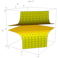
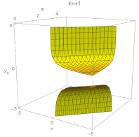
Figure 1: The variation $X_{0}$ versus typical values of the $m$ and $n$ parameters in (61) for the dust background.

3.2 Black Hole-Dust Background Field Interactions

For the dust surrounding field, we set the equation of state parameter of the dust field as $\omega_{d}=0$ [50, 126]. Then, the metric (17) takes the following form

$$ds^{2}=-\left(1-\frac{2M(u)+N_{d}(u)}{r}\right)du^{2}+2\epsilon dudr+r^{2}d\Omega^{2},$$ (63)

where $N_{d}(u)$ denotes the normalization parameter for the dust field surrounding the back hole, with the dimension of $\left[N_{d}\right]=l$ where $l$ denotes the length. It is seen that the effectively radiating-accreting black hole in the dust background appears as an effectively radiating-accreting black hole with an effective mass $M_{eff}(u)=2M(u)+N_{d}(u)$. In this case, the presence of new mass term changes the thermodynamics, causal structure and Penrose diagrams just up to a re-scaling in the original Vaidya solution.

The radiation-accretion density in the dust background is given by

$$\sigma(u,r)=\epsilon\left(\frac{2\dot{M}(u)+\dot{N}_{d}(u)}{r^{2}}\right).$$ (64)

For the Vaidya’s original solution in an empty background, i.e $N_{d}(u)=0$, or even in a static background, i.e $\dot{N}_{d}(u)=0$, the positive energy density condition, i.e $\sigma(u,r)\geq 0$, requires that $\epsilon$ and $\dot{M}(u)$ always have the same signs. This means that for $\epsilon=+1$, $M(u)$ is a monotone increasing mass function while for the case of $\epsilon=-1$, $M(u)$ is a monotone decreasing mass function. In our general solution for the Vaidya black hole in the dust background, the condition $\sigma(u,r)\geq 0$ imposed on (64) is satisfied for more general situations indicated in the Table 3.

$\epsilon$	$\dot{M}$	$\dot{N}_{d}$	Condition	Physical Process
-1	-	-	No Condition	Accretion/Decay of SF by Evaporating/Vanishing BH
-1	+	-	$|\dot{N}_{d}(u)|\geq|2\,\dot{M}(u)|$	Accretion of SF by BH
-1	-	+	$|\dot{N}_{d}(u)|\leq|2\,\dot{M}(u)|$	Absorbtion of BH’s radiation by SF
+1	+	-	$|\dot{N}_{d}(u)|\leq|2\,\dot{M}(u)|$	Accretion of SF by BH
+1	-	+	$|\dot{N}_{d}(u)|\geq|2\,\dot{M}(u)|$	Absorbtion of BH’s radiation by SF
+1	+	+	No Condition	Accretion of BH and SF

Table 3: BH and its surrounding dust field parameters for $\epsilon=\pm 1$. For these cases, the positive energy condition is satisfied everywhere in spacetime.

Interestingly, for the special case of $\dot{N}_{d}(u)=-2\dot{M}(u)$, there is no pure radiation-accretion density, i.e $\sigma(u,r)=0$, and the energy-momentum tensor (4) will be diagonalized. This means that the black hole and its surrounding background completely cancel out the effects of each others. For $\dot{N}_{d}(u)\neq-2\dot{M}(u)$, regarding (64), we find that for $r_{*}\rightarrow\infty$, the radiation-accretion density vanishes, i.e $\sigma(u,r)\rightarrow 0$. This means that for the effective emission case, the out going radiation can penetrate through the dust background so far from the black hole and for the effective accretion case by the black hole, the black hole affect its so far surrounding objects. Regrading the conditions in the Table 3 for $\epsilon=-1$ and $\epsilon=+1$, the behaviour of radiation-accretion density $\sigma$ in (64) is plotted for some typical values of $\dot{M}$ and $\dot{N}_{d}$ in the Figure 2. Using these plots, one can compare the radiation-accretion density values for the various situations.

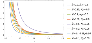
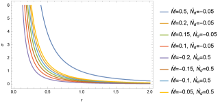
Figure 2:
Left Fig: The radiation-accretion density $\sigma$ versus the distance $r$ for some typical constant values of $\dot{M}$ and $\dot{N}_{d}$ for $\epsilon=-1$ in the dust background. The four upper cases and the four lower cases correspond to the conditions $|\dot{N}_{d}(u)|\geq|2\,\dot{M}(u)|$ and $|\dot{N}_{d}(u)|\leq|2\,\dot{M}(u)|$, respectively. By these conditions, it is clear that $\sigma(r)$ is a decreasing function but is positive, and consequently the positive energy condition is satisfied everywhere in spacetime.
Right Fig. The radiation-accretion density $\sigma$ versus the distance $r$ for some typical constant values of $\dot{M}$ and $\dot{N}_{d}$ for $\epsilon=+1$ in the dust background. The four upper cases and the four lower cases correspond to the conditions $|\dot{N}_{d}(u)|\leq|2\,\dot{M}(u)|$ and $|\dot{N}_{d}(u)|\geq|2\,\dot{M}(u)|$, respectively. By these conditions, it is clear that $\sigma(r)$ is a decreasing function but is positive, and consequently the positive energy condition is satisfied everywhere in spacetime.

3.3 Timelike Geodesics for the Black Hole in the Dust Field Background

For this case, we have $D_{s_{1}}=D_{s_{2}}$ and both the particular situations associated with $|\frac{a_{s_{1}}}{a_{N}}|\simeq 1$ and $|\frac{a_{s_{2}}}{a_{L}}|\simeq 1$ are met for $M(u)=\frac{|N_{d}(u)|}{2}$ in the whole spacetime. In Figure 3, we have plotted the possibility of being these particular situations for some typical ranges of $M(u)$ and $N_{d}(u)$ parameters. Then, one realizes the possibility of equality of the Newtonian force as well as GR correction terms to the corresponding dust background field contributions.

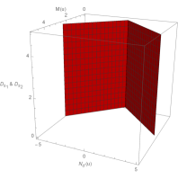
Figure 3: The variation of $D_{s_{1}}$ and $D_{s_{2}}$ versus typical values of the $M(u)$ and $N_{d}(u)$ parameters for the dust background.

Also, for this case, the equation (60) associated with $a_{i}\simeq a_{N}$ takes the following form

$$\mathfrak{L}+\frac{1}{2}\mathfrak{N}\simeq MR^{-1}.$$ (65)

One can find the following solutions to (65)

$$R\simeq\frac{2M}{2\mathfrak{L}+\mathfrak{N}}.$$ (66)

Then, one realizes that how this particular distance depends on the parameters $\mathfrak{L},\mathfrak{N}$ and $M$. In the Figure 4, we have plotted the solutions of (65) for some typical ranges of $\mathfrak{L}$ and $\mathfrak{N}$ parameters. This figure indicates that depending the parameter values, there are locations where the induced force, resulting from the radiation-accretion phenomena in the dust background, is equal to the Newtonian gravitational force.

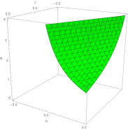
Figure 4: The variation of $R$ versus typical values of the $\mathfrak{L}$ and $\mathfrak{N}$ parameters in (65) for the dust background. We have set $M=1$ without loss of generality.

4 Evaporating-Accreting Vaidya Black Hole Surrounded by the Radiation Field

4.1 Naked Singularity or Black Hole Formation Analysis

For this case, the equation (43) takes the following form

$$nX_{0}^{3}+2mX_{0}^{2}-X_{0}+2\epsilon=0.$$ (67)

Then, we obtain the following solutions to (67)

$$X_{01}=-\frac{2m}{3n}-\frac{-4m^{2}-3n}{3n\Delta}+\frac{\Delta}{3n},$$

$$X_{02}=-\frac{2m}{3n}+\frac{(1+i\sqrt{3})(-4m^{2}-3n)}{6n\Delta}-\frac{(1-i\sqrt{3})\Delta}{6n},$$

$$X_{03}=-\frac{2m}{3n}+\frac{(1-i\sqrt{3})(-4m^{2}-3n)}{6n\Delta}-\frac{(1+i\sqrt{3})\Delta}{6n},$$ (68)

where $\Delta$ is given by

$$\Delta=\Delta_{-}=\left(-8m^{3}-9mn+27n^{2}+3\sqrt{3}\sqrt{-m^{2}n^{2}-16m^{3}n^{2}-n^{3}-18mn^{3}+27n^{4}}\right)^{\frac{1}{3}},\leavevmode\nobreak\ \leavevmode\nobreak\ \epsilon=-1,$$

$$\Delta=\Delta_{+}=\left(-8m^{3}-9mn-27n^{2}+3\sqrt{3}\sqrt{-m^{2}n^{2}+16m^{3}n^{2}-n^{3}+18mn^{3}+27n^{4}}\right)^{\frac{1}{3}},\leavevmode\nobreak\ \leavevmode\nobreak\ \epsilon=+1.$$ (69)

Then, one finds that some particular conditions are needed on the parameters $m$ and $n$ for having positive or negative solutions. In Figure 5, we have plotted the solutions of (67) for some typical ranges of $m$ and $n$ parameters. This figure indicates the possibility of the formation of both the naked singularities and black holes in the radiation background depending on the value of parameters.

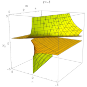
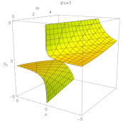
Figure 5: The variation of $X_{0}$ versus typical values of the $m$ and $n$ parameters in (67) for the radiation background.

4.2 Black Hole-Radiation Background Field Interactions

For the radiation surrounding field, we set the equation of state parameter of the radiation field as $\omega_{r}=\frac{1}{3}$ [50, 126]. Then, the metric (17) takes the following form

$$ds^{2}=-\left(1-\frac{2M(u)}{r}-\frac{N_{r}(u)}{r^{2}}\right)du^{2}+2\epsilon dudr+r^{2}d\Omega^{2},$$ (70)

where $N_{r}(u)$ is the normalization parameter for the radiation field surrounding the black hole, with the dimension of $[N_{r}]=l^{2}$. Regarding the positive energy condition on the surrounding radiation field, represented by the relation (16), it is required that $N_{r}(u)\leqslant 0$. Then, by defining the positive parameter $\mathcal{N}_{r}(u)=-N_{r}(u)$, we have

$$ds^{2}=-\left(1-\frac{2M(u)}{r}+\frac{\mathcal{N}_{r}(u)}{r^{2}}\right)du^{2}+2\epsilon dudr+r^{2}d\Omega^{2}.$$ (71)

This metric looks like a radiating charged Vaidya black, namely the Bonnor-Vaidya black hole [34], with the dynamical charge $Q(u)=\sqrt{\mathcal{N}_{r}(u)}$, see also [43] for the radiating dyon solution. This result can be interpreted as the positive contribution of the characteristic feature of the surrounding radiation field to the effective charge term of the Vaidya black hole with the $\frac{1}{r^{2}}$ gravitational contribution. The appearance of an effective charge in the black hole solution changes the causal structure and Penrose diagrams of this black hole solution in comparison to the neutral Vaidya black holes. A similar effect in the causal structure of spacetime happens when one adds charge to the static Schwarzschild black hole leading to Reissner-Nordström black hole. Then, turning off the background radiation field which surrounds the dynamical Vaidya black hole is equal to turning off the charge in the static Reissner-Nordström case.

In this case, the total radiation-accretion density is given by

$$\sigma(u,r)=\epsilon\left(\frac{2\dot{M}(u)}{r^{2}}-\frac{\mathcal{\dot{N}}_{r}(u)}{r^{3}}\right).$$ (72)

Then, we see that there is no positive $r_{*}(u)$ for $\dot{M}(u)$ and $\mathcal{\dot{N}}_{r}(u)$ having opposite signs, and consequently $\sigma(u,r)$ never vanishes except at infinity. But as $r_{*}\rightarrow\infty$, the radiation-accretion density again vanishes, i.e $\sigma(u,r_{*})\rightarrow 0$. This means that for the emission case, the out going radiation can penetrate through the radiation background so far from the black hole and for the accretion case by the black hole, the black hole affects its so far surrounding radiation filed. The positivity condition of $\sigma(u,r)$ is satisfied everywhere for the situations present in the Table 4.

$\epsilon$	$\dot{M}$	$\mathcal{\dot{N}}_{r}$	Physical Process
-1	-	+	Absorbtion of BH’s radiation by SF
+1	+	-	Accretion of SF by BH

Table 4: BH and its surrounding radiation field parameters for $\epsilon=\pm 1$. For these cases, the positive energy condition is satisfied everywhere in spacetime. For any other behaviour of the $\dot{M}(u)$ and $\mathcal{\dot{N}}_{r}(u)$ parameters, the positive energy condition will be violated.

Regrading the Table 4, the behaviour of radiation-accretion density $\sigma$ in (72) is plotted for some typical values of $\dot{M}$ and $\mathcal{\dot{N}}_{r}$ in Figure 6. Using these plots, one can compare the radiation-accretion densities for the various situations.

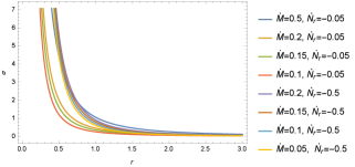
Figure 6:
Left Fig. The radiation-accretion density $\sigma$ versus the distance $r$ for some typical constant $\dot{M}$ and $\mathcal{\dot{N}}_{r}$ values for $\epsilon=-1$ in the radiation background. Here, $\sigma(r)$ is a decreasing function but is positive, and consequently the positive energy condition is satisfied everywhere in spacetime.
Right Fig. The radiation-accretion density $\sigma$ versus the distance $r$ for some typical constant $\dot{M}$ and $\mathcal{\dot{N}}_{r}$ values for $\epsilon=+1$ in the radiation background. Here, $\sigma(r)$ is a decreasing function but is positive, and consequently the positive energy condition is satisfied everywhere in spacetime.

4.3 Timelike Geodesics for the Black Hole in the Radiation Field Background

For this case, the distances $D_{s_{1}}$ and $D_{s_{2}}$ associated with $|\frac{a_{s_{1}}}{a_{N}}|\simeq 1$ and $|\frac{a_{s_{2}}}{a_{L}}|\simeq 1$, respectively, will be given by

$$D_{s_{1}}=\frac{|N_{r}(u)|}{M(u)},\leavevmode\nobreak\ \leavevmode\nobreak\ \leavevmode\nobreak\ \leavevmode\nobreak\ \leavevmode\nobreak\ D_{s_{2}}=\frac{2|N_{r}(u)|}{3M(u)}.$$ (73)

In Figure 7, we have plotted the location of these particular distances versus some typical ranges of $M(u)$ and $N_{r}(u)$ parameters. Then, one realizes the possibility of equality of the Newtonian force and GR correction terms to the corresponding radiation background field contributions.

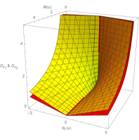
Figure 7: The variation of $D_{s_{1}}$ (yellow plot) and $D_{s_{2}}$ (red plot) versus typical values of the $M(u)$ and $N_{r}(u)$ parameters for the radiation background.

Moreover, for this case, the equation (60) associated with $a_{i}\simeq a_{N}$ takes the following form

$$\mathfrak{L}R+\frac{1}{2}\mathfrak{N}\simeq M.$$ (74)

Then, one can find the following solutions to (74)

$$R\simeq\frac{2M-\mathfrak{N}}{2\mathfrak{L}}.$$ (75)

It is seen that how this particular distance depends on the parameters $\mathfrak{L},\mathfrak{N}$ and $M$. In Figure 8, we have plotted the solutions of (74) for some typical ranges of $\mathfrak{L}$ and $\mathfrak{N}$ parameters. This figure shows that depending the parameter values, there are locations where the induced force, resulting from the radiation-accretion phenomena in the radiation background, is equal to the Newtonian gravitational force.

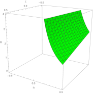
Figure 8: The variation of $R$ versus typical values of the $\mathfrak{L}$ and $\mathfrak{N}$ parameters in (65) for the radiation background. We have set $M=1$ without loss of generality.

5 Evaporating-Accreting Vaidya Black Hole Surrounded by the Quintessence Field

5.1 Naked Singularity or Black Hole Formation Analysis

For this case, the equation (43) takes the following form

$$n+2mX_{0}^{2}-X_{0}+2\epsilon=0.$$ (76)

Then, one can find the solutions as

$$X_{01}=\frac{1-\sqrt{1+16m-8mn}}{4m},\leavevmode\nobreak\ \leavevmode\nobreak\ \leavevmode\nobreak\ X_{02}=\frac{1+\sqrt{1+16m-8mn}}{4m},\leavevmode\nobreak\ \leavevmode\nobreak\ \epsilon=-1,$$

$$X_{01}=\frac{1-\sqrt{1-16m-8mn}}{4m},\leavevmode\nobreak\ \leavevmode\nobreak\ \leavevmode\nobreak\ X_{02}=\frac{1+\sqrt{1-16m-8mn}}{4m},\leavevmode\nobreak\ \leavevmode\nobreak\ \epsilon=+1.$$ (77)

Similarly, some particular conditions are required on the parameters $m$ and $n$ for having positive or negative solutions. In Figure 9, we have plotted the solutions of (76) for some typical ranges of $m$ and $n$ parameters. Then, regarding this figure, one realizes the possibility of the formation of both naked singularities and black holes in the quintessence background depending on the value of parameters.

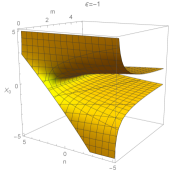
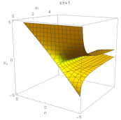
Figure 9: The variation $X_{0}$ versus typical values of the $m$ and $n$ parameters in (9) for the quintessence background.

5.2 Black Hole-Quintessence Background Field Interactions

In the cosmological context, the quintessence filed is known as the simplest scalar field dark energy model without having theoretical problems such as Laplacian instabilities or ghosts. The energy density and the pressure profile of the quintessence filed are generally considered to vary with time and depend on the scalar field and the potential, which are given by $\rho=\frac{1}{2}\dot{\phi}^{2}+V(\phi)$ and $p=\frac{1}{2}\dot{\phi}^{2}-V(\phi)$, respectively. Then, the associated equation of state parameter for quintessence field lies in the range $-1<\omega_{q}<-\frac{1}{3}$. The static Schwarzschild black hole solution surrounded by a quintessence field was found by Kiselev [50]. This solution was generalized to the charged case and studied in [136, 137, 138].

For the quintessence surrounding field, we set the equation of state parameter of quintessence field as $\omega_{q}=-\frac{2}{3}$ [50, 126]. Then, the metric (17) takes the following form

$$ds^{2}=-\left(1-\frac{2M(u)}{r}-N_{q}(u)r\right)du^{2}+2\epsilon dudr+r^{2}d\Omega^{2},$$ (78)

where $N_{q}(u)$ is the normalization parameter for the quintessence field surrounding the black hole, with the dimension of $[N_{q}]=l^{-1}$. This result shows a non-trivial contribution of the characteristic feature of the surrounding quintessence field to the metric of the Vaidya black hole. The presence of the background quintessence filed changes the causal structure and Penrose diagrams of this black hole solution in comparison to the black hole in an empty background. A rather similar effect happens when one immerses an static Schwarzschild in a (anti)-de Sitter background with the difference that here the spacetime tends asymptotically to quintessence rather than (anti)-de Sitter asymptotics.

Regarding the positive energy condition for the quintessence background, represented by the relation (16), it is required to have $N_{q}(u)\geqslant 0$. The radiation density is given by

$$\sigma(u,r)=\epsilon\left(\frac{2\dot{M}(u)}{r^{2}}+\dot{N}_{q}(u)\right).$$ (79)

Then, the dynamical behaviour of the background quintessence field is governed by

$$\begin{cases}\dot{N}_{q}(u)\leq-\,\frac{2}{r^{2}}\,\dot{M}(u),\leavevmode\nobreak\ \leavevmode\nobreak\ \leavevmode\nobreak\ &\epsilon=-1,\\ \\ \dot{N}_{q}(u)\geq-\frac{2}{r^{2}}\,\dot{M}(u),&\epsilon=+1.\end{cases}$$ (80)

Consequently, at any distance $r$ from the black hole, the surrounding quintessence field must obey the above conditions. Interestingly, for the special case of $\dot{N}_{q}(u)=-\frac{2\dot{M}(u)}{r^{2}}$, there is no pure radiation-accretion density, i.e $\sigma(u,r)=0$. This case corresponds to two possible physical situations. The first one is related to the situation where observer can be located at any distance $r$ such that the quintessence background’s and black hole’s contributions cancel out each others leading to $\sigma(u,r)=0$ for a moment or even a period of time. Then, it is required that for an evaporating black hole, we have an equal absorbing quintessence background or for an accreting black hole we have an equal accreted quintessence background. The second situation is related to the case that for the given dynamical behaviors of the black hole and its quintessence background, one can find the particular distance $r_{*}=\sqrt{-\frac{2\dot{M}(u)}{\dot{N}_{q}(u)}}$ possessing zero energy density. For $|\dot{N}_{q}(u)|\ll|\dot{M}(u)|$, we have $r_{*}\rightarrow\infty$. This indicates that for an evolving black hole in an almost static quintessence background, the positive energy condition is satisfied everywhere. Also, the positivity of $r_{*}$ also requires that $\dot{M}(u)$ and $\dot{N}_{q}(u)$ have opposite signs. Then, if one realize the black and its surrounding quintessence filed behaviors, i.e $\dot{M}(u)$ and $\dot{N}_{q}(u)$ values, he can find a distance at which we have no any radiation-accretion energy density contribution. Based on these possibilities, the various situations in the Table 5 can be realized.

$\epsilon$	$\dot{M}$	$\dot{N}_{q}$	$r_{*}$	$\sigma({r<r_{*}})$	$\sigma({r=r_{*}})$	$\sigma({r>r_{*}})$	Physical Process
-1	-	-	Imaginary	+	+	+	Accretion/Decay of SF by Evaporating/Vanishing BH
-1	+	-	+	-	0	+	Accretion of SF by BH
-1	-	+	+	+	0	-	Absorbtion of BH’s radiation by SF
+1	-	+	+	-	0	+	Absorbtion of BH’s radiation by SF
+1	+	-	+	+	0	-	Accretion of SF by BH
+1	+	+	Imaginary	+	+	+	Accretion of BH and SF

Table 5: BH and its surrounding quintessence field parameters for $\epsilon=\pm 1$. For the quintessence background, the positive energy condition may be completely or partially respected regarding to the above situations.

Then, regarding this table, the positive values of $r_{*}$ are physically viable and their corresponding physical processes are listed in the last column. These properties are determined according to the behaviours of the parameters $\epsilon$, $\omega_{q}$, and quantities $\dot{M}(u)$, $\dot{N}_{q}(u)$, and $\sigma(u,r)$. Those values of $r_{*}$ corresponding to the negative energy density $\sigma(u,r)$ represent no physical situation about the evaporation-absorption or accretion. The real features of those regions are hidden by the weak energy condition. In the reference [125], the accretion into a static Kiselev black hole with a static exterior spacetime surrounded by a quintessence field without the back-reaction effect is studied. The obtained results in [125] are implying that the accretion rate and the critical points depend on the background quintessence parameter $N_{q}$. Then, these features deserve to be incorporated in astrophysical studies of the accretion processes.

Regrading the Table 5, the behaviour of radiation-accretion density $\sigma$ in (79) is plotted for some typical values of $\dot{M}$ and $\dot{N}_{q}$ in Figure 3. Using these plots, one can compare the radiation-accretion densities for the various situations.

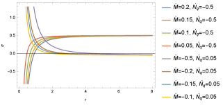
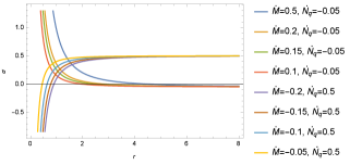
Figure 10:
Left Fig. The radiation-accretion density $\sigma$ versus the distance $r$ for some typical constant $\dot{M}$ and $\dot{N}_{q}$ values for $\epsilon=-1$ in the quintessence background. In the four upper cases, the accretion density is an increasing function from negative to the positive values. In the four lower cases, the radiation density is a decreasing function decreases from positive values to negative values. Then, for a dynamical quintessence background, if the condition $|\dot{N}_{q}(u)|\ll|\dot{M}(u)|$ is not met, the positive energy condition is violated in some regions of spacetime.
Right Fig. The radiation-accretion density $\sigma$ versus the distance $r$ for some typical constant $\dot{M}$ and $\dot{N}_{q}$ values for $\epsilon=+1$ in the quintessence background. In the upper panel, the accretion density is a decreasing function from positive to the negative values. In the lower panel, the radiation density is an increasing function from negative values to positive values. Then, for a dynamical quintessence background, if the condition $|\dot{N}_{q}(u)|\ll|\dot{M}(u)|$ is not met, the positive energy condition is violated in some regions of spacetime.

5.3 Timelike Geodesics for the Black Hole in the Quintessence Field Background

For this case, the distances $D_{s_{1}}$ and $D_{s_{2}}$ associated with $|\frac{a_{s_{1}}}{a_{N}}|\simeq 1$ and $|\frac{a_{s_{2}}}{a_{L}}|\simeq 1$, respectively, are given as

$$D_{s_{1}}^{2}=\frac{2M(u)}{|-N_{q}(u)|},\leavevmode\nobreak\ \leavevmode\nobreak\ \leavevmode\nobreak\ \leavevmode\nobreak\ \leavevmode\nobreak\ D_{s_{2}}^{2}=\frac{6M(u)}{|N_{q}(u)|}.$$ (81)

In Figure 19, we have plotted the location of these particular distances for some typical ranges of the black hole mass $M(u)$ and background quintessence field $N_{q}(u)$ parameters. Then, one finds that there are possibilities for the equality of the Newtonian force and GR correction terms to the corresponding quintessence background field contributions.

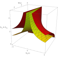
Figure 11: The variation of $D_{s_{1}}$ (yellow plot) and $D_{s_{2}}$ (red plot) versus typical values of the $M(u)$ and $N_{q}(u)$ parameters for the quintessence background.

The equation (60) associated with $a_{i}\simeq{a_{N}}$ for this case takes the following form

$$\mathfrak{L}R^{-2}+\frac{1}{2}\mathfrak{N}\simeq MR^{-3}.$$ (82)

Then, we obtain the following solutions

$$R_{1}\simeq-\frac{2\mathfrak{L}}{3^{\frac{1}{3}}\left(9M\mathfrak{N}^{2}+\sqrt{3}\sqrt{8\mathfrak{L}^{3}\mathfrak{N}^{3}}+27M^{2}\mathfrak{N}^{4}\right)^{\frac{1}{3}}}+\frac{\left(9M\mathfrak{N}^{2}+\sqrt{3}\sqrt{8\mathfrak{L}^{3}\mathfrak{N}^{3}}+27M^{2}\mathfrak{N}^{4}\right)^{\frac{1}{3}}}{3^{\frac{2}{3}}\mathfrak{N}},$$

$$R_{2}\simeq\frac{(1+i\sqrt{3})\mathfrak{L}}{3^{\frac{1}{3}}\left(9M\mathfrak{N}^{2}+\sqrt{3}\sqrt{8\mathfrak{L}^{3}\mathfrak{N}^{3}}+27M^{2}\mathfrak{N}^{4}\right)^{\frac{1}{3}}}-\frac{(1-i\sqrt{3})\left(9M\mathfrak{N}^{2}+\sqrt{3}\sqrt{8\mathfrak{L}^{3}\mathfrak{N}^{3}}+27M^{2}\mathfrak{N}^{4}\right)^{\frac{1}{3}}}{2\times 3^{\frac{2}{3}}\mathfrak{N}},$$

$$R_{3}\simeq\frac{(1-i\sqrt{3})\mathfrak{L}}{3^{\frac{1}{3}}\left(9M\mathfrak{N}^{2}+\sqrt{3}\sqrt{8\mathfrak{L}^{3}\mathfrak{N}^{3}}+27M^{2}\mathfrak{N}^{4}\right)^{\frac{1}{3}}}-\frac{(1+i\sqrt{3})\left(9M\mathfrak{N}^{2}+\sqrt{3}\sqrt{8\mathfrak{L}^{3}\mathfrak{N}^{3}}+27M^{2}\mathfrak{N}^{4}\right)^{\frac{1}{3}}}{2\times 3^{\frac{2}{3}}\mathfrak{N}}.$$

Then, one finds that the location of this particular distance depends on the parameters $\mathfrak{L},\mathfrak{N}$ and $M$. In Figure 12, we have plotted the solutions of (82) for some typical ranges of $\mathfrak{L}$ and $\mathfrak{N}$ parameters. This figure shows that depending the parameter values, there are locations where the induced force, resulting from the radiation-accretion phenomena in the quintessence background, is equal to the Newtonian gravitational force.

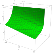
Figure 12: The variation of $R$ versus typical values of the $\mathfrak{L}$ and $\mathfrak{N}$ parameters in (65) for the quintessence background. We have set $M=1$ without loss of generality.

6 Evaporating-Accreting Vaidya Black Hole Surrounded by the Cosmological Constant

6.1 Naked Singularity or Black Hole Formation Analysis

For this case, the equation (43) takes the following form

$$nX_{0}^{-1}+2mX_{0}^{2}-X_{0}+2\epsilon=0.$$ (84)

Then, one can find the following solutions to (84)

$$X_{01}=\frac{1}{6m}-\frac{-1-12m}{3\times 2^{\frac{2}{3}}m\Delta}+\frac{\Delta}{6\times 2^{\frac{1}{3}}m},$$

$$X_{02}=\frac{1}{6m}+\frac{(1+i\sqrt{3})(-1-12m)}{6\times 2^{\frac{2}{3}}m\Delta}-\frac{(1-i\sqrt{3})\Delta}{12\times 2^{\frac{1}{3}}m},$$

$$X_{03}=\frac{1}{6m}+\frac{(1-i\sqrt{3})(-1-12m)}{6\times 2^{\frac{2}{3}}m\Delta}-\frac{(1+i\sqrt{3})\Delta}{12\times 2^{\frac{1}{3}}m},$$ (85)

where $\Delta$ is given by

$$\Delta=\Delta_{-}=\left(2+36m-108m^{2}n+\sqrt{4(-1-12m)^{3}+(2+36m-108m^{2}n)^{2}}\right)^{\frac{1}{3}},\leavevmode\nobreak\ \leavevmode\nobreak\ \epsilon=-1,$$

$$\Delta=\Delta_{+}=\left(2-36m-108m^{2}n+\sqrt{4(-1+12m)^{3}+(2-36m-108m^{2}n)^{2}}\right)^{\frac{1}{3}},\leavevmode\nobreak\ \leavevmode\nobreak\ \epsilon=+1.$$ (86)

Then, one see that some particular conditions on the parameters $m$ and $n$ are required for having positive or negative solutions. In Figure 13, we have plotted the solutions of (84) for some typical ranges of $m$ and $n$ parameters. Then, regarding this figure, one realizes the possibility of the formation of the both the naked singularities and black holes in the cosmological constant-like background depending on the value of parameters.

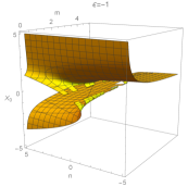
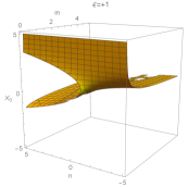
Figure 13: The variation $X_{0}$ versus typical values of the $m$ and $n$ parameters in (84) for the cosmological constant-like background.

6.2 Black Hole-Cosmological Background Field Interactions

For the cosmological constant-like surrounding field, we set the equation of state parameter of the cosmological field as $\omega_{c}=-1$ [50, 126]. Then, the metric (17) takes the following form

$$ds^{2}=-\left(1-\frac{2M(u)}{r}-N_{c}(u)r^{2}\right)du^{2}+2\epsilon dudr+r^{2}d\Omega^{2},$$ (87)

where $N_{c}(u)$ is the normalization parameter for the cosmological field surrounding the black hole, with the dimension of $[N_{c}(u)]=l^{-2}$. This result indicates the non-trivial contribution of the characteristic feature of the surrounding cosmological constant to the metric of the Vaidya black hole. The presence of the background cosmological field changes the causal structure and Penrose diagrams of this black hole solution in comparison to the black hole in an empty background. This is similar to the case of the static Schwarzschild black hole in a static de Sitter background such that the Penrose diagram changes from Schwarzschild to Schwarzschild-(anti) de Sitter. Then, in our case, the Penrose diagram changes from Vaidya to Vaidya-de Sitter case with dynamical cosmological causal boundaries.

Regarding the positive energy condition for this case, represented by the relation (16), it is required to have $N_{c}(u)\geqslant 0$. In this case, $N_{c}(u)$ plays the role of a positive dynamical cosmological constant. Then, this case may describes the dynamical black holes in more general cosmological scenarios considering a time varying cosmological term, which have been recently proposed in the literature. The main purpose of these cosmological models is to provide an explanation for the recent accelerating phase of the universe [127]-[135]. These models are well known as the $\Lambda(t)$, where $t$ is the cosmic time. For the case of $N_{c}=constant=\Lambda$, we recover the solution of the Vaidya black hole embedded in a de Sitter space obtained in [42]. The evolutionary behaviour of such an evaporating black hole including the structures, locations and dynamics of the apparent and event horizons are studied in [108].

In this case, the radiation-accretion density is given by

$$\sigma(u,r)=\epsilon\left(\frac{2\dot{M}(u)}{r^{2}}+\dot{N}_{c}(u)r\right).$$ (88)

Then, the dynamical behaviour of the background cosmological constant-like field is governed by

$$\begin{cases}\dot{N}_{c}(u)\leq-\frac{2}{r^{3}}\,\dot{M}(u),\leavevmode\nobreak\ \leavevmode\nobreak\ \leavevmode\nobreak\ &\epsilon=-1,\\ \\ \dot{N}_{c}(u)\geq-\frac{2}{r^{3}}\,\dot{M}(u),&\epsilon=+1.\end{cases}$$ (89)

Consequently, at any distance $r$ from the black hole, the surrounding cosmological field must obey the above conditions. Similar to the previous solution, for the special case of $\dot{N}_{c}(u)=-\frac{2\dot{M}(u)}{r^{3}}$, there is no pure radiation-accretion density, i.e $\sigma(u,r)=0$. This case corresponds to two possible physical situations. The first one is related to the situation where observer can be located at any distance $r$ such that the cosmological background’s and black hole’s contributions cancel out each others leading to $\sigma(u,r)=0$ for a moment or even a period of time. Then, it is required that for a radiating black hole, we have an equal absorbing cosmological background or for an accreting black hole we have an equal accreted cosmological background field. The second situation is related to the case that for the given dynamical behaviors of the black hole and its cosmological background, one can find the particular distance $r_{*}=\left(-\frac{2\dot{M}(u)}{\dot{N}_{c}(u)}\right)^{\frac{1}{3}}$ possessing zero energy density. For $|\dot{N}_{c}(u)|\ll|\dot{M}(u)|$, we have $r_{*}\rightarrow\infty$. This indicates that for an evolving black hole in an almost static cosmological background, the positive energy condition is respected everywhere. Here also, the positivity of $r_{*}$ also guarantees that $\dot{M}(u)$ and $\dot{N}_{c}(u)$ have opposite signs. Then, if one realize the black and its surrounding cosmological filed behaviors, i.e $\dot{M}(u)$ and $\dot{N}_{c}(u)$ values, he can find a distance at which we have no any radiation-accretion energy density contribution. Based on these possibilities, the various situations in the Table 6 can be realized.

$\epsilon$	$\dot{M}$	$\dot{N}_{c}$	$r_{*}$	$\sigma({r<r_{*}})$	$\sigma({r=r_{*}})$	$\sigma({r>r_{*}})$	Physical Process
-1	-	-	-	+	+	+	Accretion/Decay of SF by Evaporating/Vanishing BH
-1	+	-	+	-	0	+	Accretion of SF by BH
-1	-	+	+	+	0	-	Absorbtion of BH’s radiation by SF
+1	-	+	+	-	0	+	Absorbtion of BH’s radiation by SF
+1	+	-	+	+	0	-	Accretion of SF by BH
+1	+	+	-	+	+	+	Accretion of BH and SF

Table 6: BH and its surrounding cosmological field parameters for $\epsilon=\pm 1$. For the cosmological background, the positive energy condition may be completely or partially respected regarding to the above situations.

Regrading the Table 6, the behaviour of radiation-accretion density $\sigma$ in (88) is plotted for some typical values of $\dot{M}$ and $\dot{N}_{c}$ in Figure 4. Using these plots, one can compare the radiation-accretion densities for the various situations.

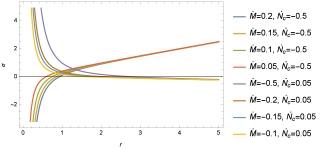
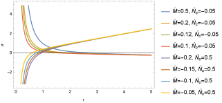
Figure 14:
Left Fig. The radiation-accretion density $\sigma$ versus the distance $r$ for some typical constant values $\dot{M}$ and $\dot{N}_{c}$ values for $\epsilon=-1$ in the cosmological background. In the four upper cases, the accretion density is an increasing function from negative to positive values. In the four lower cases, the radiation density is a decreasing function from positive values to negative values. Then, for a dynamical cosmological background, if the condition $|\dot{N}_{c}(u)|\ll|\dot{M}(u)|$ is not met, the positive energy condition is violated in some regions of spacetime.
Right Fig. The radiation-accretion density $\sigma$ versus the distance $r$ for some typical constant values $\dot{M}$ and $\dot{N}_{c}$ values for $\epsilon=+1$ in the cosmological background. In the four upper cases, the accretion density is a decreasing function from positive to negative values. In the four lower cases, the radiation density is an increasing function from negative to positive values. Then, for a dynamical cosmological background, if the condition $|\dot{N}_{c}(u)|\ll|\dot{M}(u)|$ is not met, the positive energy condition is violated in some regions of spacetime.

6.3 Timelike Geodesics for the Black Hole in the Cosmological Constant-Like Field Background

For this case, the distances $D_{s_{1}}$ and $D_{s_{2}}$ associated with $|\frac{a_{s_{1}}}{a_{N}}|\simeq 1$ and $|\frac{a_{s_{2}}}{a_{L}}|\simeq 1$, respectively, read as

$$D_{s_{1}}^{3}=\frac{M(u)}{|-N_{q}(u)|},\leavevmode\nobreak\ \leavevmode\nobreak\ \leavevmode\nobreak\ \leavevmode\nobreak\ \leavevmode\nobreak\ D_{s_{2}}\rightarrow\infty.$$ (90)

The case of $D_{s_{2}}\rightarrow\infty$ is resulting from the fact that, in contrast to black hole itself, the cosmological constant-like field does not couple to angular momentum $L$, see $a_{s_{2}}$ in (56). This shows that there is no similar effect to the GR correction term for the cosmological constant-like field. In Figure 19, we have plotted the location of the particular distance $D_{s_{1}}$ for some typical ranges of the black hole mass $M(u)$ and background cosmological constant-like field $N_{c}(u)$ parameters. Then, one finds that there are possibilities for the equality of the Newtonian force to the corresponding cosmological constant-like background field contributions.

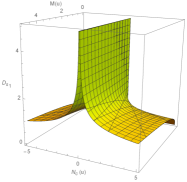
Figure 15: The variation of $D_{s_{1}}$ versus typical values of the $M(u)$ and $N_{c}(u)$ parameters for the cosmological constant-like background.

For this case, the equation (60) associated with $a_{i}\simeq a_{N}$ takes the form of

$$\mathfrak{L}R^{-3}+\frac{1}{2}\mathfrak{N}\simeq MR^{-4}.$$ (91)

Then, we arrive at the following solutions

$$R_{1}\simeq\frac{1}{2}\Delta^{\frac{1}{2}}-\frac{1}{2}\sqrt{-\Delta-\frac{4\mathfrak{L}}{\mathfrak{N}\Delta^{\frac{1}{2}}}},$$

$$R_{2}\simeq\frac{1}{2}\Delta^{\frac{1}{2}}+\frac{1}{2}\sqrt{-\Delta-\frac{4\mathfrak{L}}{\mathfrak{N}\Delta^{\frac{1}{2}}}},$$

$$R_{3}\simeq-\frac{1}{2}\Delta^{\frac{1}{2}}-\frac{1}{2}\sqrt{-\Delta+\frac{4\mathfrak{L}}{\mathfrak{N}\Delta^{\frac{1}{2}}}},$$

$$R_{4}\simeq-\frac{1}{2}\Delta^{\frac{1}{2}}+\frac{1}{2}\sqrt{-\Delta+\frac{4\mathfrak{L}}{\mathfrak{N}\Delta^{\frac{1}{2}}}},$$

where $\Delta$ is

$$\Delta=-\frac{4\times 2^{\frac{2}{3}}M}{3^{\frac{1}{3}}\left(9\mathfrak{L}^{2}\mathfrak{N}+\sqrt{3}\sqrt{27\mathfrak{L}^{4}\mathfrak{N}^{2}}+128M^{3}\mathfrak{N}^{3}\right)^{\frac{1}{3}}}+\frac{2^{\frac{1}{3}}\left(9\mathfrak{L}^{2}\mathfrak{N}+\sqrt{3}\sqrt{27\mathfrak{L}^{4}\mathfrak{N}^{2}}+128M^{3}\mathfrak{N}^{3}\right)^{\frac{1}{3}}}{3^{\frac{2}{3}}\mathfrak{N}}.$$ (93)

Again, we see that how the solutions of this particular distance depends on the parameters $\mathfrak{L},\mathfrak{N}$ and $M$. In Figure 16, we have plotted the solutions of (91) for some typical ranges of $\mathfrak{L}$ and $\mathfrak{N}$ parameters. This figure shows that depending the parameter values, there are locations where the induced force, resulting from the radiation-accretion phenomena in the cosmological background, is equal to the Newtonian gravitational force.

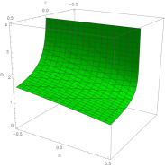
Figure 16: The variation of $R$ versus typical values of the $\mathfrak{L}$ and $\mathfrak{N}$ parameters in (65) for the cosmological constant-like background. We have set $M=1$ without loss of generality.

7 Evaporating-Accreting Vaidya Black Hole Surrounded by the Phantom Field

7.1 Naked Singularity or Black Hole Formation Analysis

For this case, the equation (43) takes the following form

$$nX_{0}^{-2}+2mX_{0}^{2}-X_{0}+2\epsilon=0.$$ (94)

Then, one can find the following solutions to this equation

$$X_{01}=\frac{1}{8m}-\frac{1}{2}\Delta^{\frac{1}{2}}-\frac{1}{2}\sqrt{\frac{3}{16m^{2}}+\frac{6}{3m}-\Delta-\frac{\frac{1}{8m^{3}}-\frac{2}{m^{2}}}{4\Delta^{\frac{1}{2}}}},$$

$$X_{02}=\frac{1}{8m}-\frac{1}{2}\Delta^{\frac{1}{2}}+\frac{1}{2}\sqrt{\frac{3}{16m^{2}}+\frac{6}{3m}-\Delta-\frac{\frac{1}{8m^{3}}-\frac{2}{m^{2}}}{4\Delta^{\frac{1}{2}}}},$$

$$X_{03}=\frac{1}{8m}+\frac{1}{2}\Delta^{\frac{1}{2}}-\frac{1}{2}\sqrt{\frac{3}{16m^{2}}+\frac{6}{3m}-\Delta+\frac{\frac{1}{8m^{3}}-\frac{2}{m^{2}}}{4\Delta^{\frac{1}{2}}}},$$

$$X_{04}=\frac{1}{8m}+\frac{1}{2}\Delta^{\frac{1}{2}}+\frac{1}{2}\sqrt{\frac{3}{16m^{2}}+\frac{6}{3m}-\Delta+\frac{\frac{1}{8m^{3}}-\frac{2}{m^{2}}}{4\Delta^{\frac{1}{2}}}},$$ (95)

where $\Delta$ is given by

$$\Delta = \Delta_{-}=\frac{1}{16m^{2}}+\frac{2}{3m}+\frac{2\times 2^{\frac{1}{3}}(1+6mn)}{3m\left(-16+27n+288mn+\sqrt{(-16+27n+288mn)^{2}-4(4+24mn)^{3}}\right)^{\frac{1}{3}}}$$

$$+\frac{\left(-16+27n+288mn+\sqrt{(16+27n+288mn)^{2}-4(4+24mn)^{3}}\right)^{\frac{1}{3}}}{6\times 2^{\frac{1}{3}}m},\leavevmode\nobreak\ \leavevmode\nobreak\ \epsilon=-1,$$

$$\Delta = \Delta_{+}=\frac{1}{16m^{2}}-\frac{2}{3m}+\frac{2\times 2^{\frac{1}{3}}(1+6mn)}{3m\left(16+27n-288mn+\sqrt{(16+27n-288mn)^{2}-4(4+24mn)^{3}}\right)^{\frac{1}{3}}}$$ (96)

$$+\frac{\left(16+27n-288mn+\sqrt{(16+27n-288mn)^{2}-4(4+24mn)^{3}}\right)^{\frac{1}{3}}}{6\times 2^{\frac{1}{3}}m},\leavevmode\nobreak\ \leavevmode\nobreak\ \epsilon=+1.$$

Then, similar to the previous cases, some particular conditions on the parameters $m$ and $n$ are required for having positive or negative solutions. In Figure 17, we have plotted the solutions of (94) for some typical ranges of $m$ and $n$ parameters. Regarding this figure, we find the possibility of the formation of the both the naked singularities and black holes in the phantom background depending on the value of parameters.

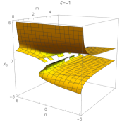
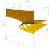
Figure 17: The variation $X_{0}$ versus typical values of the $m$ and $n$ parameters in (94) for the phantom background.

7.2 Black Hole-Phantom Background Field Interactions

For the phantom surrounding field, we set the equation of state parameter of phantom field as $\omega_{p}=-\frac{4}{3}$ [126]. Then, the metric (17) takes the following form

$$ds^{2}=-\left(1-\frac{2M(u)}{r}-N_{p}(u)r^{3}\right)du^{2}+2\epsilon dudr+r^{2}d\Omega^{2},$$ (97)

where $N_{p}(u)$ is the normalization parameter for the phantom field surrounding the black hole, with the dimension of $[N_{p}(u)]=l^{-3}$. Similarly, this result is interpreted as the non-trivial contribution of the characteristic feature of the surrounding phantom field to the metric of the Vaidya black hole. The presence of the background phantom filed changes the causal structure and Penrose diagrams of this black hole solution in comparison to the Vaidya black hole in an empty background.

Regarding the weak energy condition for this case, represented by the relation (16), it is required to have $N_{p}(u)\geqslant 0$. In this case, the radiation-accretion density is given by

$$\sigma(u,r)=\epsilon\left(\frac{2\dot{M}(u)}{r^{2}}+\dot{N}_{p}(u)r^{2}\right).$$ (98)

Then, the dynamical behaviour of the background field is governed by

$$\begin{cases}\dot{N}_{p}(u)\leq-\frac{2}{r^{4}}\,\dot{M}(u),\leavevmode\nobreak\ \leavevmode\nobreak\ \leavevmode\nobreak\ &\epsilon=-1,\\ \\ \dot{N}_{p}(u)\geq-\frac{2}{r^{4}}\dot{M}(u),&\epsilon=+1.\end{cases}$$ (99)

Consequently, at any distance $r$ from the black hole, the surrounding phantom field must obey the above conditions. Similar to the previous solutions, for the special case of $\dot{N}_{p}(u)=-\frac{2\dot{M}(u)}{r^{4}}$, there is no pure radiation-accretion density, i.e $\sigma(u,r)=0$. This case corresponds to two possible physical situations. The first one is related to the situation where observer can be located at any distance $r$ such that the phantom background’s and black hole’s contributions cancel out each others leading to $\sigma(u,r)=0$ for a moment or even a period of time. Then, it is required that for a radiating black hole, we have an equal absorbing phantom background or for an accreting black hole we have an equal accreted phantom background. The second situation is related to the case that for the given dynamical behaviors of the black hole and its phantom background, one can find the particular distance $r_{*}=\left(-\frac{2\dot{M}(u)}{\dot{N}_{p}(u)}\right)^{\frac{1}{4}}$ possessing zero energy density. Similarly, for $|\dot{N}_{p}(u)|\ll|\dot{M}(u)|$, we have $r_{*}\rightarrow\infty$. This indicates that for an evolving black hole in an almost static phantom background, the positive energy condition is satisfied everywhere. Also, the positivity of $r_{*}$ also requires that $\dot{M}(u)$ and $\dot{N}_{p}(u)$ must have opposite signs. Then, if one realize the black and its surrounding phantom filed behaviors, i.e $\dot{M}(u)$ and $\dot{N}_{p}(u)$ values, he can find a distance at which we have no any radiation-accretion energy density contribution. Based on these possibilities, the various situations in the Table 7 can be realized.

$\epsilon$	$\dot{M}$	$\dot{N}_{p}$	$r_{*}$	$\sigma({r<r_{*}})$	$\sigma({r=r_{*}})$	$\sigma({r>r_{*}})$	Physical Process
-1	-	-	Imaginary	+	+	+	Accretion/Decay of SF by Evaporating/Vanishing BH
-1	+	-	+	-	0	+	Accretion of SF by BH
-1	-	+	+	+	0	-	Absorbtion of BH’s radiation by SF
+1	-	+	+	-	0	+	Absorbtion of BH’s radiation by SF
+1	+	-	+	+	0	-	Accretion of SF by BH
+1	+	+	Imaginary	+	+	+	Accretion of BH and SF

Table 7: BH and its surrounding phantom field parameters for $\epsilon=\pm 1$. For the phantom background, the positive energy condition may be completely or partially respected regarding to the above situations.

Specific scenarios involving the accretion of phantom energy and resulting in the area decrease of black hole [96, 97, 98, 99] are related to the first case in the above table. For example, in [96], it is shown that the black holes will gradually vanish as the universe approaches a cosmological big rip state with a phantom field. One should note that the astrophysically “observed” infall of quintessence/phantom fields onto black holes are not detected till now. In the present work, we have just introduced a new dynamical solution to the Einstein field equations which can provide a classical model for the “possible” black hole accretion and evaporation (presumably very tiny) in different cosmological backgrounds. Such theoretical studies of the accretion of exotic fields to the black holes are well motivated by cosmology in which these exotic fields can be responsible for the current accelerating expansion of the universe. Regrading the Table 7, the behavior of radiation-accretion density $\sigma$ in (98) is plotted for some typical values of $\dot{M}$ and $\dot{N}_{p}$ in Figure 5. Using these plots, one can compare the radiation-accretion densities for the various situations.

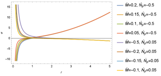
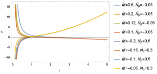
Figure 18:
Left Fig. The radiation-accretion density $\sigma$ versus the distance $r$ for some typical constant $\dot{M}$ and $\dot{N}_{p}$ values for $\epsilon=-1$ in the phantom background. In the four upper cases, the accretion density is an increasing function from negative to positive values. In the four lower cases, the radiation density is a decreasing function from positive to negative values. Then, for a dynamical phantom background, if the condition $|\dot{N}_{p}(u)|\ll|\dot{M}(u)|$ is not met, the positive energy condition is violated in some regions of spacetime.
Right Fig. The radiation-accretion density $\sigma$ versus the distance $r$ for some typical constant $\dot{M}$ and $\dot{N}_{p}$ values for $\epsilon=+1$ in the phantom background. In the four upper cases, the accretion density is a decreasing function from positive to negative values. In the four lower cases, the radiation density is an increasing function from negative to positive values. Then, for a dynamical phantom background, if the condition $|\dot{N}_{p}(u)|\ll|\dot{M}(u)|$ is not met, the positive energy condition is violated in some regions of spacetime.

7.3 Timelike Geodesics for the Black Hole in the Phantom Field Background

For this case, the distances $D_{s_{1}}$ and $D_{s_{2}}$ associated with $|\frac{a_{s_{1}}}{a_{N}}|\simeq 1$ and $|\frac{a_{s_{2}}}{a_{L}}|\simeq 1$, respectively, are given as

$$D_{s_{1}}^{4}=\frac{2M(u)}{3|-N_{p}(u)|},\leavevmode\nobreak\ \leavevmode\nobreak\ \leavevmode\nobreak\ \leavevmode\nobreak\ \leavevmode\nobreak\ D_{s_{2}}^{4}=\frac{6M(u)}{|-N_{p}(u)|}.$$ (100)

In Figure 19, we have plotted the location of these particular distances for some typical ranges of the black hole mass $M(u)$ and background phantom field $N_{p}(u)$ parameters. Then, one realizes the possibilities of the equality of the Newtonian force and GR correction terms to the corresponding phantom background field contributions.

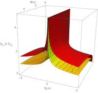
Figure 19: The variation of $D_{s_{1}}$ (yellow plot) and $D_{s_{2}}$ (red plot) versus typical values of the $M(u)$ and $N_{q}(u)$ parameters for the quintessence background.

Moreover, the equation (60) for this case takes the following form

$$\mathfrak{L}R^{-4}+\frac{1}{2}\mathfrak{N}\simeq MR^{-5}.$$ (101)

Then, we see that this produces a fifth order equation in which finding its analytical solutions is not simple. However, in Figure 20, we have shown that there are numerical solutions to (101) for some typical ranges of $\mathfrak{L}$ and $\mathfrak{N}$ parameters. This figure indicates that depending the parameter values, there are locations where the induced force, resulting from the radiation-accretion phenomena in the phantom background, is equal to the Newtonian gravitational force.

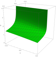
Figure 20: The variation of $R$ versus typical values of the $\mathfrak{L}$ and $\mathfrak{N}$ parameters in (101) for the phantom background. We have set $M=1$ without loss of generality.

8 Conclusion

In this work, we have studied the general surrounded Vaidya solution with the cosmological fields of dust, radiation, quintessence, cosmological constant-like and phantom, and investigated its nature describing the possibility of the formation of naked singularities or black holes. We have obtained the general equation describing the nature of the solution under a collapse, and have shown that depending on the parameter values, the formation of both naked singularity and black hole as the end state of the collapse are possible. We have given the corresponding analytical solutions as well as some plots indicating these possibilities. Then, motivated by the fact that real astrophysical black holes as non-stationary and non-isolated objects are living in non-empty backgrounds, we have focused on the black hole subclasses of the obtained general solution, namely the “surrounded Vaidya black hole”, describing a dynamical evaporating-accreting black holes in the mentioned dynamical cosmological backgrounds. In the following, we summarize some of our obtained results for this solution.

• Some of the subclasses of the obtained general solution for both the dynamical and stationary limits have been addressed. In particular, we have shown that the original Vaidya solution can be recovered by turning off the background field, and that the Kiselev static solution can be obtained in the stationary limit with an appropriate coordinate transformation. Also, the Schwarzschild solution can be obtained in the stationary limit with a turned off background.

• We have shown that for the background field possessing $\omega_{s}>0$, if $\dot{M}(u)$ and $\dot{N}_{s}(u)$ have a same order of magnitude, the surrounding background field contribution to the total density $\sigma(u,r)$ is dominant near the black hole while at far distances from the black hole it decreases faster than the contribution of the black hole mass changing term. In contrast, for the background field possessing $\omega_{s}<0$, the surrounding background field contribution is dominant at large distances while the black hole contribution is dominant near the black hole itself. Then, from astrophysical point of view, the detected amount of the radiation-accretion density by the observer not only depends on the distance from the black but also depends on the nature of background field.

• We have discussed that positive energy condition for the surrounding field is met by the constraint $\omega_{s}N_{s}(u)\leq 0$, which determines the gravitational nature of the term associated to surrounding field in the metric function $f(u,r)$. The positive energy condition for the radiation-accretion density is met by the constraints $\dot{N}_{s}(u)\leq-2\,{r}^{3\omega_{s}}\,\dot{M}(u)$ and $\dot{N}_{s}(u)\geq-2\,{r}^{3\omega_{s}}\,\dot{M}(u)$ at any distance $r$ for $\epsilon=-1$ and $\epsilon=+1$, respectively. One astrophysical importance of such physical constraints is that the observer knows the dynamical range of the background field at any distance and then prior to any observation, he knows how to include or remove the background field contribution, if he is only interested in black hole’s contributions, or vice vera.

• We have addressed the solutions of the black hole in the dust ($\omega_{s}=0$), radiation ($\omega_{s}=\frac{1}{3}$), quintessence ($\omega_{s}=-\frac{2}{3}$), cosmological constant-like ($\omega_{s}=-1$) and phantom ($\omega_{s}=-\frac{4}{3}$) fields in detail. We have found that the effectively evaporating-accreting black hole in the dust background appears as an effectively evaporating-accreting black hole with an effective mass $M_{eff}(u)=2M(u)+N_{d}(u)$. Then, the presence of new mass term changes the causal structure just up to a re-scaling in the original Vaidya solution. For the radiation background, the spacetime metric looks like the Bonnor-Vaidya and radiating dyon solutions with the dynamical charge $Q(u)=\sqrt{\mathcal{N}_{r}(u)}$. A similar effect in the causal structure of spacetime here happens when one adds charge to the static Schwarzschild black hole leading to Reissner-Nordström black hole. For the black hole in the dust and radiation backgrounds, the spacetime metrics are asymptotically flat while for the the quintessence, cosmological-like and phantom backgrounds, spacetime metrics are asymptotically non-flat quintessence, de Sitter-like and phantom, respectively. Consequently, the causal structure of these three latter spacetimes are quite different from the original Vaidya spacetime where the background is turned off.

• Regarding the obtained radiation-accretion density $\sigma(u,r)$, we have found that there are particular distances $r_{*}$ where $\sigma(u,r)$ vanishes, i.e $\sigma(u,r_{*})=0$. These distances are given by $r_{*}(u)=\left(-\frac{\dot{N}_{s}(u)}{2\dot{M}(u)}\right)^{\frac{1}{3\omega_{s}}}$ and $r_{*}=\infty$. Then, one realizes that in the first case, for $(i)$ $-\frac{2}{3}<\omega_{s}<0$ with $|\dot{N}_{s}(u)|\ll 2|\dot{M}(u)|$ and for $(ii)$ $\omega_{s}\geq 0$ with $2|\dot{M}(u)|\ll|\dot{N}_{s}(u)|$, we have $r_{*}\rightarrow\infty$. This means that for $(i),$ the black hole evolves very faster than its background while for $(ii)$, the black hole evolves very slow relative to its background. Also, for $(iii)$ $\omega_{s}\leq-\frac{2}{3}$ with $|\dot{N}_{s}(u)|\ll 2|\dot{M}(u)|$, representing a rapidly evolving black hole relative to its background, we have $r_{*}\rightarrow\infty$. Then, by satisfaction of these dynamical conditions to hold $r_{*}\rightarrow\infty$, the positive energy density is respected everywhere in the spacetime. The case $(ii)$ includes the black hole surrounded by the rapidly evolving dust and radiation fields while the cases $(i)$ and $(iii)$ imply an evolving black hole in an almost static cosmological backgrounds (quintessence, cosmological constant-like or phantom fields) responsible for the accelerating expansion of the universe. In practice, an astrophysical observer detects a radiation-accretion density resulting from the interaction of the black hole with its surrounding field even at far distances, in which for $(ii)$ the main contribution in the detected radiation-accretion density belongs to surrounding field while for $(i)$ and $(iii)$, it is the black hole which has the main contribution in the radiation-accretion density.

• In the case that there is a real, positive and finite value for $r_{*}$, the positive energy condition is violated in some regions of spacetime such that real features of those regions are hidden by the weak energy condition. Then, it is physically reasonable to do any astrophysical experiments in the regions respecting the energy condition. For the cases in which $r_{*}$ is not positive and real, the interpretation is as follows: the radiation-accretion density $\sigma(u,r)$ never and nowhere vanishes.

• We have classified the possible situations respecting or violating the energy condition for all the solutions of black hole in dust, radiation, quintessence, cosmological constant-like and phantom backgrounds in the Tables 1-7. It is shown that there are cases for all the backgrounds in which the positive energy condition is respected in whole spacetime under the determined behaviors of black hole and its surrounding field. Also, we have given some plots for radiation-accretion density versus some typical values of black hole and its surrounding fields in Figs 1-5. Using these plots, one realizes for the dust and radiation backgrounds, although the radiation-accretion density is a decreasing function but is always positive, and consequently the positive energy condition is satisfied everywhere in spacetime. This is while for the quintessence, cosmological constant-like and phantom backgrounds, if the condition $|\dot{N}_{q,c,p}(u)|\ll|\dot{M}(u)|$ is not met, the positive energy condition is violated in some regions of spacetime. Comparing the plots with common values of the parameters, we observe that the radiation-accretion density $\sigma(r)$ for the radiation background is larger than the dust background at any distance $r$, i.e $\sigma_{r}(r)>\sigma_{d}(r)$. Similarly, for the quintessence, cosmological constant-like and phantom backgrounds, we have $\sigma_{q}(r)<\sigma_{c}(r)<\sigma_{p}(r)$ for the radiation-accretion density.

• We have analyzed the timelike geodesics associated with the obtained surrounded black holes and have found that two kinds of new correction terms arise relative to the case of Schwarzschild black hole. The first kind of corrections are due to the presence of the background fields which surround the Vaidya black hole. This corrections include two terms in which its first term is similar to the term of Newtonian gravitational potential, while its second term is similar to the relativistic correction of GR. For the various background fields, we have discussed that there are possibilities for the equality of Newtonian and GR correction terms to the corresponding background fields contributions. We have given some plots denoting these possibilities for each case. The second kind of corrections is also a non-Newtonian correction resulting from the dynamics of black hole and its surrounding field. We have shown that depending on the dynamical features of black hole and its background, there are also possibilities that dynamical correction terms can be equal to the Newtonian case. Some plots representing these situations are given for each case. Then, one realizes that for the more realistic non-empty and non-static backgrounds, the geodesic equation of any object depends strictly not only on the mass of the central object of the system and the angular momentum of the orbiting body, but also on the ($i$) background field type and ($ii$) black hole and its background field dynamics.

We have reported elsewhere on the causal structures and thermodynamical properties of our obtained solutions here [139]. We also aim to generalize this work to the case of charged solutions.

References

- [1] J. Frank, A. King, D. Raine, Accretion power in astrophysics, Cambridge University Press (2002).
- [2] S.L. Shapiro, Astrophys. J. 180, 531 (1973).
- [3] S.W. Hawking, Comm. Math. Phys. 43, 199 (1975); Phys. Rev. D 14, 2460 (1976).
- [4] A. Ashtekar, B. Krishnan, Phys. Rev. D 68(10), 104030 (2003); Liv. Rev. Rel, 7(1), 10 (2004).
- [5] S.A. Hayward, Phys. Rev. D, 49(12), 6467 (1994).
- [6] P. C. Vaidya, Proc. Indian Acad. Sci. A 33, 264 (1951); P. C. Vaidya, Gen. Rel. Grav. 31, 119 (1999).
- [7] P. C. Vaidya, Current Science 12, 183 (1943).
- [8] W. A. Hiscock, Phys. Rev. D 23, 2813 (1981); W. A. Hiscock, Phys. Rev. D 23, 2823 (1981).
- [9] W. A. Hiscock, L. G. Williams, D. M. Eardley, Phys. Rev. D 26, 751 (1982).
- [10] Y. Kuroda, Prog. Theor. Phys. 71, 100 (1984); Prog. Theor. Phys. 71, 1422 (1984).
- [11] R. Parentani, Phys. Rev. D 63, 041503 (2001).
- [12] M. K. Parikh, F. Wilczek, Phys. Lett. B 449, 1 (1999).
- [13] R. Di Criscienzo, M. Nadalini, L. Vanzo, S. Zerbini, G. Zoccatelli, Phys. Lett. B 657,107 (2007).
- [14] M. O’Loughlin, Phys. Rev. D 91.4, 044020 (2015).
- [15] H.L. Li, S.Z. Yang, T.J. Zhou, R. Lin, Europhys. Lett. 84(2), 20003 (2008).
- [16] S.H. Mehdipour, Phys. Rev. D 81, 124049 (2010).
- [17] S.W. Kim, E.Y. Choi, S.K. Kim, J. Yang, Physics Letters A, 141(5-6), 238 (1989).
- [18] A.N.St.J. Farley, P.D. D’Eath, Gen. Rel. Grav. 38, 425 (2006).
- [19] Y. Zhang, W. Liu, Astrophysics and Space Science 312, no. 3-4 , 315 (2007).
- [20] S.Q. Wu, X. Cai, Int. J. Theor. Phy. 41, no. 3, 559 (2002).
- [21] Z. Zheng, L. Zhong-heng, Il Nuovo Cimento B (1971-1996), 108(7), 785 (1993).
- [22] M.I. Beciu, Phys. Lett. A 100.2, 77 (1984).
- [23] Z. Zheng, Y. Cheng-Quan, R. Qin-An, Gen. Rel. Grav. 26(11), 1055 (1994).
- [24] S. Sawayama, Phys. Rev. D 73.6, 064024 (2006).
- [25] R. Penrose, Riv. Nuovo Cimento 1, 252 (1969).
- [26] S. G. Ghosh, N. Dadhich, Phys. Rev. D 64, 047501 (2001).
- [27] T. Harko, Phys. Rev. D 68, 064005 (2003).
- [28] I. H. Dwivedi, P. S. Joshi, Class. Quant. Grav 6.11, 1599(1989).
- [29] I.H. Dwivedi, P.S. Joshi, Class. Quant. Grav 6.11, 1599 (1989).
- [30] Y. Kuroda, Y. Prog. Theor. Phys. 72(1), 63 (1984).
- [31] T. Harko, Phys. Rev. D 68, 064005 (2003).
- [32] W.A. Hiscock, L.G. Williams, D.M. Eardley, Phys. Rev. D 26, 751, (1982).
- [33] C. Vaz, L. Witten, Phys. Lett. B 442, 90 (1998).
- [34] W. B. Bonnor, P. C. Vaidya, Gen. Rel. Grav. I, 2, 127 (1970).
- [35] B. T. Sullivan, W. Israel, Phys. Lett. A79, 371 (1980).
- [36] Y. Kaminaga, Class. Quant. Grav. 7, 1135 (1990).
- [37] A. Patino, H. Rago, Phys. Lett. A 121, 329 (1987).
- [38] S. Wanglin, L. Xingye, W. Li, Z. Qingxiang, Nucl. Phys. B (Proc. Suppl.) 166, 270 (2007).
- [39] L. Xiang, Z. Zheng, Phys. Rev. D 62, 104001 (2000).
- [40] A. Wang, Y. Wu, Gen. Rel. Grav. 31.1, 107 (1999).
- [41] S. W. Hawking, G. F. R. Ellis,The Large Scale Structure of Spacetime, Cambridge University Press, Cambridge, England (1973).
- [42] R. L. Mallett, Phys. Rev. D, 31(2), 416 (1985).
- [43] A. Chamorro, K. S. Virbhadra, Pramana 45.2, 181 (1995).
- [44] R. L. Mallett, Phys. Lett. A, 126(4), 226 (1988).
- [45] A. Patino, H. Rago, Phys. Lett. A 121, 329 (1987).
- [46] R. L. Mallet, Phys. Lett. A 126, 226 (1988).
- [47] B. Koberlein, R. L. Mallet, Phys. Rev. D 49, 5111 (1994).
- [48] H. Saida, T. Harada, H. Maeda, Class. Quant. Grav. 24, 4711 (2007).
- [49] V. Husain, Phys. Rev. D 53, 1759 (1996).
- [50] V. V. Kiselev, Class. Quant. Grav. 20, 1187 (2003).
- [51] R. Geroch and J.B. Hartle, J. Math. Phys. 23, 680 (1982).
- [52] S. Fairhurst, B. Krishnan, Int. J. Mod. Phys. D10, 691 (2001).
- [53] S.R. Brandt, E. Seidel, Phys. Rev. D54, 1403 (1996).
- [54] M. Ansorg, D. Petroff, Phys. Rev. D 72.2, 024019 (2005).
- [55] S. W. Hawking, Commun. Math. Phys. 25, 152 (1972).
- [56] J.D. Brown and V. Husian, Int. J. Mod. Phys. D6, 563 (1997).
- [57] S.Droz, M. Heusler, N. Straumann, Phys. Lett. B, 268(3-4), 371 (1991).
- [58] J. Barranco, A. Bernal, J.C. Degollado, A. Diez-Tejedor, M. Megevand, M. Alcubierre, D.Núñez, O. Sarbach, Phys. Rev. Lett. 109, 081102 (2012).
- [59] J.D. Bekenstein, Phys. Rev. D 51(12), R6608 (1995).
- [60] M. Rizwan, M. Jamil, A. Wang, arXiv:1802.04301.
- [61] S. L. Shapiro, S. A. Teukolsky, Black holes, white dwarfs and neutron stars: the physics of compact objects, John Wiley Sons (2008).
- [62] J. Frank, A. King, D. Raine, Accretion power in astrophysics, Cambridge University Press (2002).
- [63] S. K. Chakrabarti, Theory of transonic astrophysical flows, World Scientific, Vol. 150 (1990).
- [64] F. H. Shu, The Physics of Astrophysics: Gas Dynamics, University Science Books, Vol 2 (1991).
- [65] L. C. Ho, Coevolution of Black Holes and Galaxies, Carnegie Observatories Astrophysics Series, Vol.1, Cambridge (2004).
- [66] L. Rezzolla, O. Zanotti, Relativistic Hydrodynamics, Oxford University Press, New York (2013).
- [67] F. Hoyle, R.A. Lyttleton, Proc. Camb. Philos. Soc. 35, 405 (1939).
- [68] S. Bahamonde, M. Jamil, Eur. Phys. J. C 75, 508 (2015).
- [69] H. Bondi, F. Hoyle, Mon. Not. R. Astron. Soc. 104, 273 (1944).
- [70] H. Bondi, Mon. Not. R. Astron. Soc. 112, 195 (1952).
- [71] F.C. Michel, Astrophys. Space. Sci. 15, 153 (1972).
- [72] S. L. Shapiro, Astrophys. J. 180, 531 (1973).
- [73] S. L. Shapiro, Astrophys. J. 185, 69 (1973).
- [74] S. L. Shapiro, Astrophys. J. 189, 343 (1974).
- [75] E. Malec, Phys. Rev. D 60, 104043 (1999).
- [76] R. Bousso, Phys. Rev. D 71, 064024 (2005).
- [77] S.G. Ghosh, Eur. Phys. J. C 76. 4, 222 (2016).
- [78] S. Chen, J. Jing, Class. Quant. Grav. 22.21, 4651 (2005).
- [79] Y. Zhang, Y.X. Gui, Class. Quant. Grav. 23.22, 6141 (2006).
- [80] N. Varghese, V.C. Kuriakose, Gen. Rel. Grav. 41.6, 1249 (2009).
- [81] K. Ghaderi, B. Malakolkalami, Nucl. Phys. B 903, 10 (2016).
- [82] B. Majeed, M. Jamil, P. Pradhan, Adv. High Energy Phys. 2015 (2015).
- [83] M. Azreg-Aïnou, M.E. Rodrigues, JHEP 2013.9, 146 (2013).
- [84] B. B. Thomas, M. Saleh, T.C. Kofane, Gen. Rel. Grav. 44.9, 2181 (2012).
- [85] M. Jamil, S. Hussain, B. Majeed, Eur. Phys. J. C 75. 1, 24 (2015).
- [86] I. Hussain, S. Ali, Eur. Phys. J.l Plus 131. 8, 275 (2016).
- [87] B. Malakolkalami, K. Ghaderi, Mod. Phys. Lett. A 30.10, 1550049 (2015).
- [88] S. Fernando, Gen. Rel. Grav. 44.7, 1857 (2012).
- [89] R. Uniyal, N.C. Devi, H. Nandan, K.D. Purohit, Gen. Rel. Grav. 47.2, 16 (2015).
- [90] S. Fernando, S. Meadows, K. Reis, Int. J. Theo. Phys. 54.10, 3634 (2015).
- [91] L. Jiao, R. Yang, Eur. Phys. J. C 77, 356 (2017).
- [92] M. Azreg-Aïnou, S. Bahamonde, M. Jamil, Eur. Phys. J. C 77.6 414 (2017).
- [93] J. Barranco, A. Bernal, J. C. Degollado, A. Diez-Tejedor, M. Megevand, M. Alcubierre, D. Núñez, O. Sarbach, Phys. Rev. Lett. 109, 081102 (2012).
- [94] E. O. Babichev, V. I. Dokuchaev, Yu. N. Eroshenko, Phys. Usp. 56, 1155 (2013).
- [95] F. Ficek, Class. Quant. Grav. 32, 235008 (2015).
- [96] E. O. Babichev, V. I. Dokuchaev, Yu. N. Eroshenko, Phys. Rev. Lett. 93, 021102 (2004).
- [97] E. O. Babichev, V. I. Dokuchaev, Yu. N. Eroshenko, J. Exp. Theor. Phys. 100, 528 (2005).
- [98] L. H. Ford, T. A. Roman, Phys. Rev. D 64, 024023 (2001).
- [99] C. Gao, X. Chen, V. Faraoni, Y.-G. Shen, Phys. Rev. D78, 024008 (2008).
- [100] M. G. Rodrigues, A. Saa, Phys. Rev. D 80, 104018 (2009).
- [101] J. A. González, F. S. Guzmán, Phys. Rev. D 79, 121501 (2009); J. A. González, F. S. Guzmán, Phys. Rev. D 94, 104012 (2016).
- [102] James M. Cline, Sangyong Jeon, Guy D. Moore Phys. Rev. D 70, 043543 (2004).
- [103] M. Jamil, A. Qadir, M.A. Rashid, Eur. Phys. J. C 58, 325 (2008).
- [104] L. A. Ureña-López, L.M. Fernández, Phys. Rev. D 84, 044052 (2011).
- [105] J. Barranco, A. Bernal, J. C. Degollado, A. Diez-Tejedor,M. Megevand, M. Alcubierre, D. Núñez, O. Sarbach, Phys. Rev. D 89, 083006 (2014).
- [106] Y. Heydarzade, F. Darabi, Phys. Lett. B, 771, 365 (2017).
- [107] R. W. Lindquist, R. A. Schwartz, C. W. Misner, Physical Review 137, 5B (1965).
- [108] R. L. Mallet, Phys. Rev. D 33, 2201 (1986); Erratum Phys. Rev. D 34, 664 (1986).
- [109] D. Vick, Lett. Nuovo Cimento, 44, 127 (1985).
- [110] S-W. Kim, Phys. Lett. A 141, 5 (1989).
- [111] J. W. York, Phys. Rev. D 28, 2929 (1983).
- [112] Z. Zheng, L. Zhong-heng, Nuovo Cimento B 108, 785 (1993).
- [113] S. G. Ghosh, N. Dadhich, Phys. Rev. D 64, 047501 (2001).
- [114] R-G. Cai, L-M. Cao, Y-P. Hu, S. P. Kim, Phys. Rev. D 78, 124012 (2008).
- [115] J-R. Ren, R. Li, Mod. Phys. Lett. A 23, 3265 (2008).
- [116] E. Abdalla, C. B. M. H. Chirenti, A. Saa, Phys. Rev. D 74, 084029 (2006).
- [117] S. H. Mehdipour, Phys. Rev. D 81, 124049 (2010).
- [118] S. Zhou, W. Liu, Mod. Phys. Lett. A 24, 2099 (2009).
- [119] B. D. Koberlin, R. L. Mallet, Phys. Rev. D 49, 5111 (1994).
- [120] U. Debnath, N. C. Chakraborty, S. Chakraborty, Gen. Rel. Grav. 40.4, 749 (2008).
- [121] K. D. Patil, U. S. Thool, Int. J. M. P. D 14.05, 873 (2005).
- [122] B. Creelman, I. Booth, Phys. Rev. D 95.12, 124033 (2017).
- [123] P. Rudra, R. Biswas, U. Debnath, Astrophys. Space. Sci 354, 597 (2014).
- [124] R. W. Lindquist, R. A. Schwartz, C. W. Misner, Phys. Rev., 137(5B), B1364 (1965).
- [125] L. Jiao, R. Yang, arXiv:1605.02320.
- [126] A. Vikman, Phys. Rev. D 71, 023515 (2005).
- [127] O. Bertolami, Nuovo Cim. B 93, 36 (1986).
- [128] M. Ozer, M.O. Taha, Nucl. Phys. B 287, 776 (1987).
- [129] K. Freese, F. C. Adams, J. A. Frieman, E. Mottola, Nucl. Phys. B 287, 797 (1987).
- [130] P. J. E. Peebles, B. Ratra, Astrophys. J. 325, L17 (1988).
- [131] V. Silveira, I. Waga, Phys. Rev. D 56, 4625 (1997).
- [132] R. Opher, A. Pelinson, Phys. Rev. D 70, 063529 (2004).
- [133] J.S. Alcaniz, J. A. S. Lima, Phys. Rev. D 72, 063516 (2005).
- [134] F. Darabi, Astrophys. Space Sci. 338, 171 (2012).
- [135] S. H. Pereira, S. S. A. Pinho, J. M. H. Silva, J. F. Jesusb, JCAP 01, 055 (2017).
- [136] K. Ghaderi, B. Malakolkalami, Nucl. Phys. B 903, 10 (2016); K. Ghaderi, B. Malakolkalami, Astrophys. Space. Sci 361, 161 (2016).
- [137] B. Majeed, M. Jamil, P. Pradhan, Adv. High. Energy. Phys. 2015, 124910 (2015).
- [138] M. Azreg-Aïnou, S. Bahamonde, M. Jamil, Eur. Phys. J. C77, 414 (2017).
- [139] Y. Heydarzade, F. Darabi, Eur. Phys. J. C (2018) 78:342