Integration through transients for inelastic hard sphere fluids

Abstract

We compute the rheological properties of inelastic hard spheres in steady shear flow for general shear rates and densities. Starting from the microscopic dynamics we generalise the Integration Through Transients (itt) formalism to a fluid of dissipative, randomly driven granular particles. The stress relaxation function is computed approximately within a mode-coupling theory—based on the physical picture, that relaxation of shear is dominated by slow structural relaxation, as the glass transition is approached. The transient build-up of stress in steady shear is thus traced back to transient density correlations which are computed self-consistently within mode-coupling theory. The glass transition is signalled by the appearance of a yield stress and a divergence of the Newtonian viscosity, characterizing linear response. For shear rates comparable to the structural relaxation time, the stress becomes independent of shear rate and we observe shear thinning, while for the largest shear rates Bagnold scaling, i.e., a quadratic increase of shear stress with shear rate, is recovered. The rheological properties are qualitatively similar for all values of $\varepsilon$, the coefficient of restitution; however, the magnitude of the stress as well as the range of shear thinning and thickening show significant dependence on the inelasticity.

I Introduction

Understanding the rheology of granular fluids from a kinetic theory point of view has been of interest from the earliest days of granular physics Bagnold (1954); Haff (1983); Walton and Braun (1986); Campbell (1990); Jaeger and Nagel (1992); Iverson (1997); Brey et al. (1998); Savage (1998). It has been established that the granular Boltzmann, or Boltzmann-Enskog equation Brilliantov and Pöschel (2004); Goldshtein and Shapiro (1995) is a useful starting point to understand granular gases at low density Campbell (1990); Goldshtein and Shapiro (1995); Brey et al. (1998); Goldhirsch (2003); Brilliantov and Pöschel (2004); Vollmayr-Lee et al. (2011). Various methods to extract the transport coefficients in linear response, originally developed for molecular gases have been generalized to non-equilibrium granular gases Brey et al. (1998); Garzó and Montanero (2002); Jenkins and Richman (1985); Garzó (2013). The general understanding is that the Navier-Stokes equations of hydrodynamics (with small modifications Dufty (2007)) provide a useful description of granular gas flow. Unfortunately, the range of natural phenomena involving flow at low density and infinitesimal perturbations is much smaller for granular media than it is for classical gas flow. Most granular flows occur at both high volume fraction and significant shear rates. Indeed every gravity driven granular flow will start from a granular solid at rest Jaeger et al. (1996); Iverson (1997); Kokelaar et al. (2017) with a packing fraction around the random close packing density of the respective material. Only recently, first proposals to extend granular kinetic theory to relevant densities have appeared Reddy and Kumaran (2007); Kumaran (2014); Suzuki and Hayakawa (2014); Kranz and Sperl (2017); Jenkins and Berzi (2017).

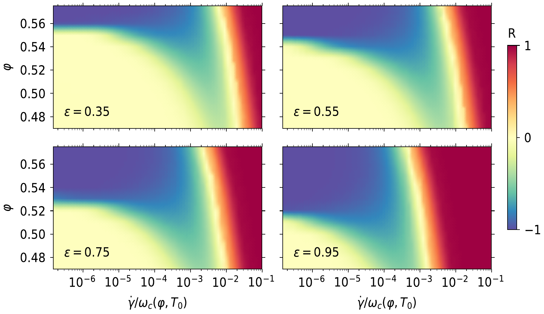
Figure 1: Protocol H (Shear heating increases the granular temperature): Dynamic state diagrams in the plane spanned by shear rate, $\dot{\gamma}$, and packing fraction, $\varphi$, for several values of the coefficient of restitution, $\varepsilon$, as indicated. The effective exponent $R$ quantifying the shear rate dependence of the viscosity, $\eta(\dot{\gamma})\sim{\dot{\gamma}}^{R}$, is color coded. Shear thickening (thinning) corresponds to $R>0$ ($R<0$) while $R=0$ indicates Newtonian behavior. The shear rate is normalized by the collision frequency $\omega_{c}(\varphi,T_{0})$ of the unsheared system (at granular temperature $T_{0}$) with the prescribed volume fraction. The data for all figures is available as Supplemental Material sup .

Qualitative considerations have shown that the dynamic state diagram characterizing the rheological response of a granular fluid to shear (Fig. 1) is determined by several timescales Kranz et al. (2018). The Newtonian behavior—where shear stress $\sigma=\eta\dot{\gamma}$ is linearly related to the shear rate $\dot{\gamma}$—extends to higher densities and shear rates as long as the shear rate is smaller than the intrinsic structural relaxation rate $\tau_{\alpha}^{-1}$. Beyond that, the shear stress becomes approximately independent of shear rate, indicated by shear thinning behavior. For even higher shear rates, shear heating will become important which appears as shear thickening behavior. Ultimately, Bagnold scaling, $\sigma\sim{\dot{\gamma}}^{2}$, holds for the largest shear rates.

In this contribution we will introduce a kinetic theory, namely the granular Integration Through Transients (gitt) formalism that is tailored to high densities and arbitrary shear rates of an intrinsically out-of-equilibrium granular fluid. To be precise, gitt is expected to be most accurate close to the granular glass transition Abate and Durian (2006); Kranz et al. (2010); Gholami et al. (2011); Avila et al. (2016), i.e., for packing fractions $\varphi$ in the range $0.5\lesssim\varphi\lesssim 0.6$. In addition, gitt is not an expansion around zero shear and also not limited to almost elastic particles. Our approach is based on the itt formalism for thermalized colloidal dispersions Fuchs and Cates (2002, 2009); Chong and Kim (2009); Brader et al. (2009); Nicolas and Fuchs (2016) and provides a framework to calculate flow curves, i.e., shear stress $\sigma$ as a function of shear rate $\dot{\gamma}$, beyond the linear response regime. To keep the paper at a manageable length we will use the simplest assumptions and point out possible refinements for future work.

A first generalization of the itt formalism from the overdamped Brownian dynamics of colloidal suspensions to inertial, Newtonian dynamics has been obtained by Chong and Kim (2009) and later updated to the refined formulation of Fuchs and Cates (2009) by Suzuki and Hayakawa (2013). In both cases the lack of viscous damping in the inertial description necessitates the explicit introduction of a thermostat. At least for the Gaussian isokinetic thermostat Evans and Morriss (1990) used in the above references, the details of the artificial thermostat explicitly appear in the final results. Suzuki and Hayakawa (2014) were the first employing an itt calculation for inelastic soft spheres. Unexpectedly, they found that no dissipative effects remain after applying the standard itt approximations. Only after including current correlation functions in addition to the density correlator did they find results that depend on the inelasticity of the particles. The substantially increased complexity due to the additional observables has so far made applications of this approach difficult. On the upside, employing dissipative interactions removes the need for an artificial thermostat.

In the following we will show that using frictionless inelastic hard spheres, it is much simpler to retain dissipative effects and this allows us to develop a granular itt formalism that captures the qualitative behavior introduced above. The paper is organized as follows. We will start with an informal outline of the model and derivations in Sec. II. Subsequently in Sec. III, we introduce the microscopic equations of motion and the observables, i.e., correlation functions. The generalized Green-Kubo relations that form the central part of the granular itt formalism (gitt) will be derived in Sec. IV. To evaluate the Green-Kubo relations, we need to compute the transient correlator approximately in mode-coupling theory, as discussed in Sec. V. In Sec. VI we will present a number of results that can be derived from the formalism developed here before concluding in Sec. VII.

II Outline of the Derivation and Main Assumptions

As the following derivation comprises a number of technical steps, requiring a set of assumptions and approximations, we are going to outline the main steps of the derivation here informally, pointing to the relevant details in the later sections. We restrict our analysis to the simplest model that captures the essential physics and relegate the discussion of some exemplary extensions to Sec. VII.

Starting from a quiescent granular fluid, beginning at time $t=0$ we impose a shear profile of the form $\bm{u}(\bm{r})=\bm{r}\cdot\mathsf{k}$ with a velocity gradient tensor $\mathsf{k}$ which is given by $k_{\alpha\beta}=\dot{\gamma}\delta_{\alpha x}\delta_{\beta y}$. To compute the shear stress $\sigma(\dot{\gamma})$, we work along the following roadmap:

1. Specify the stationary state of the quiescent fluid

2. Specify the stationary state of the sheared fluid which is reached for asymptotically long times

3. Generalize the Green-Kubo relation and integration through transients to granular fluids

4. Couple stress and structural relaxation

5. Compute the transient correlations within mode-coupling approximation

II.1 The Quiescent State

We consider a granular fluid comprised of $N$ monodisperse frictionless inelastic hard spheres of diameter $d$, mass $m=1$ and density $n=N/V$. The inelasticity is modeled by a constant coefficient of normal restitution $\varepsilon\in[0,1)$ Haff (1983); Aspelmeier et al. (2001). Note that the incomplete restitution in collision breaks time reversal symmetry. We assume that despite the monodispersity the system will not crystallize at any time. This choice is motivated by the observation that a small amount of polydispersity, just enough to prevent crystallization Schöpe et al. (2007), does not qualitatively alter the behavior of hard sphere fluids but only yields small quantitative corrections Hunter and Weeks (2012). Considering the monodisperse limit simplifies the calculations, though. Note, however, that the quiescent fluid undergoes a granular glass transition to an amorphous solid above a critical packing fraction $\varphi_{c}(\varepsilon)$ Abate and Durian (2006); Kranz et al. (2010); Sperl et al. (2012); Kranz et al. (2013). Away from the jamming transition, macroscopic granular particles are well approximated by hard-core interactions. Considerable particle deformations are expected to become relevant in violent flow conditions with very high impact speeds which consequently fall outside of our model.

The only intrinsic length scale in the system is the particle diameter $d$ and the only energy scale is given by the granular temperature $T$ (we set the Boltzmann constant $k_{B}=1$ throughout). The quiescent fluid therefore comprises a single time scale that may be given as the inverse of the collision frequency $\omega_{c}\propto\sqrt{T}/d$ Chapman and Cowling (1970). The dimensionless measure of density is the packing fraction $\varphi:=\pi nd^{3}/6$.

Considering molecular or colloidal fluids it is natural to assume that shear is applied to a quiescent state in thermal equilibrium. For a granular system, there is no such uniquely defined quiescent fluid. In order to have a stationary granular fluid even before shear is applied, we imagine the granular system to be under the influence of a homogeneous driving force. Realization of such a driving force include fluidization by air Ojha et al. (2004); Taghipour et al. (2005); Born et al. (2017) or water Schröter et al. (2005). To concentrate on the granular aspects of the rheology, we do not attempt to model the driving mechanism in any detail. Instead we assume that it results in a homogeneous random driving force that injects a prescribed amount of power, $P_{D}$, into the system to compensate the energy dissipated in inelastic collisions Williams and MacKintosh (1996); Kranz et al. (2010); Fiege et al. (2009). The granular temperature, $T_{0}$, of the quiescent fluid is then implicitly given by the power balance Brilliantov and Pöschel (2004); Pagonabarraga et al. (2001); Garzó and Montanero (2002); Fiege et al. (2009); Kranz et al. (2010),

$$P_{D}=\Gamma\omega_{c}(T_{0})T_{0},$$ (1)

between driving and dissipation. Here $\Gamma=\Gamma(\varphi,\varepsilon)$ is nothing but the dimensionless dissipation rate .

The itt formalism, discussed below, allows to express ensemble averages in the strongly sheared stationary state as expectation values with respect to the phase space distribution of a quiescent reference fluid, $\varrho_{\mathrm{ref}}$. In thermal equilibrium, the quiescent fluid is described by the canonical distribution. Currently, a theoretical framework to determine $\varrho_{\mathrm{ref}}$, comparable to the framework of statistical ensembles in thermal equilibrium, does not exist. Only the marginal one-particle velocity distribution function $\varrho_{v}^{(1)}(\bm{c})$ is well characterized Brilliantov and Pöschel (2004). It is non-Gaussian but with rapidly decaying tails, $\ln\varrho_{v}^{(1)}(c\to\infty)\propto-c^{3/2}$ and its dominant contribution can be expressed as an expansion in Sonine polynomials around a Gaussian Brilliantov and Pöschel (2004). The exponentially decaying tails guarantee that the second moment of the velocity distribution exists and the quiescent reference fluid displays a well defined granular temperature:

$$T_{0}:=\frac{1}{3}\left\langle\bm{c}^{2}\right\rangle,$$ (2)

where the angular brackets denote the phase space average with respect to $\varrho_{\mathrm{ref}}$.

The most severe approximation we make is to factorize the phase space distribution into a positional and a velocity part $\varrho_{\mathrm{ref}}\approx\varrho_{r}^{(N)}(\bm{r}_{1},\ldots,\bm{r}_{N})\varrho_{v}^{(N)}(\bm{c}_{1},\ldots,\bm{c}_{N})$ although correlations are known to exist Pagonabarraga et al. (2001). Here $\bm{r}_{i}$ denotes the particles’ positions and $\bm{c}_{i}$ their peculiar velocities [cf. Eq. (13a)]. Let us stress that in the itt formalism we only need an explicit expression for $\varrho_{\mathrm{ref}}$ in the unsheared state. The strong anisotropy of the distribution of relative collisional velocities $\bm{c}_{ij}$ with respect to the impact parameter in the sheared stationary state of a granular fluid Kumaran (2009a), are—although an interesting observation—unrelated to our factorization approximation. We furthermore assume the precollisional velocity distribution to factorize in particles,

$$\varrho_{v}^{(N)}(\bm{c}_{1},\ldots,\bm{c}_{N})=\prod_{i=1}^{N}\varrho_{v}^{(1)}(\bm{c}_{i}).$$ (3)

While the postcollisional velocities are certainly highly correlated, this is a less severe approximation for the precollisional velocities Lutsko (1996, 2001). Moreover we effectively assume a Gaussian form, $\varrho_{v}^{(1)}(\bm{c})\propto\exp(-\bm{c}^{2}/2T)$. Note, however, that in many places we only need the second moment of the distribution regardless of its overall form.

The spatial structure of a dense granular fluid has received comparably little attention. A structure factor theory for granular fluids has not been developed to the best of our knowledge. Simulations and experiments in two dimensions Puglisi et al. (2012) indicate relatively modest deviations from the equilibrium hard sphere structure. Keeping to the simplest approximations, we assume the spatial structure in the granular fluid to be identical to the structure of an elastic hard sphere fluid in thermal equilibrium, $\varrho_{r}^{(N)}(\bm{r}_{1},\ldots,\bm{r}_{N})\propto\prod_{j<k}\Theta(r_{jk}-d)$. In summary, we effectively assume the phase space distribution (but not the dynamics!) in the quiescent fluid to be of canonical form.

II.2 Stationary State of the Sheared Fluid

In contrast to colloidal suspensions where the particles are embedded in a host fluid that acts as a heat bath, the granular fluid is not necessarily thermostated. Once shear is applied, the work expended to sustain the shear flow injects additional energy into the fluid. In colloidal suspensions under normal conditions, this additional shear heating, $\sigma\dot{\gamma}$ (naturally defined per volume), is readily absorbed by the heat bath and the thermodynamic temperature of the suspensions remains constant. For the granular fluid we are going to consider two protocols that deal in different ways with the additional shear heating :

Protocol H

keeping the driving power, $P_{D}$, fixed between the quiescent and the sheared fluid such that the shear heating increases the total injected power, $P_{D}+\sigma\dot{\gamma}/n=\Gamma\omega_{c}(T)T$. Using Eq. (1) to eliminate $P_{D}$, the power balance may be rewritten as

$$\sigma\dot{\gamma}+n\Gamma\omega_{c}(T_{0})T_{0}=n\Gamma\omega_{c}(T)T.$$ (4)

The granular temperature in the sheared stationary state $T>T_{0}$ will necessarily be elevated compared to the quiescent fluid.

Protocol T

keeping the total injected power fixed, i.e., reducing the driving power in the sheared fluid $P_{D}^{\dot{\gamma}}<P_{D}$, such that $P_{D}^{\dot{\gamma}}+\sigma\dot{\gamma}/n=P_{D}$. Note that this effective thermostatting can only work as long as the shear heating is smaller than the initial driving power, $\sigma\dot{\gamma}\leq nP_{D}$, i.e., it only applies up to a maximum shear rate $\dot{\gamma}_{\infty}$. For admissible shear rates, however, the granular temperature in the sheared stationary state $T\equiv T_{0}$ will remain unchanged from the quiescent fluid.

Note that gitt formalism developed below is not limited to these simple protocols. More complicated power balances can easily be incorporated.

The time scale set by the shear rate $\dot{\gamma}$ is to be compared to the intrinsic time scale, defining the dimensionless Péclet number $\operatorname{Pe}:=\dot{\gamma}/\omega_{c}(T)$. Besides the coefficient of restitution $\varepsilon$, the only two parameters which control the rheology Kranz et al. (2018) are $\varphi$ and $\operatorname{Pe}$. A dimensionless shear stress is naturally defined as $\hat{\sigma}=\hat{\sigma}(\operatorname{Pe};\varphi,\varepsilon):=\sigma/nT$, independent of the granular temperature $T$. At low density, $\varphi\ll 1$, and small shear rate, $\dot{\gamma}\to 0$, we expect Newtonian rheology Kranz et al. (2018),

$$\sigma(\varphi\ll 1)=:\sigma_{0}=\eta\dot{\gamma},$$ (5)

with a viscosity $\eta(\varphi\ll 1)$ that is well approximated by the Enskog predictions, $\eta_{E}(\varphi,\varepsilon)$, of Garzó and Montanero (2002).

Solving Eq. (4) for the granular temperature $T$ in the sheared stationary state of Protocol H, one finds

$$T(\operatorname{Pe})=\frac{T_{0}}{(1-\operatorname{Pe}/\operatorname{Pe}_{\infty})^{2/3}},$$ (6)

where $\operatorname{Pe}_{\infty}$ is the maximum admissible Péclet number implicitly defined by Kranz et al. (2018)

$$\operatorname{Pe}_{\infty}=\Gamma/\hat{\sigma}(\operatorname{Pe}_{\infty}).$$ (7)

Note that the stationary granular temperature $T$ diverges as $\operatorname{Pe}\to\operatorname{Pe}_{\infty}$, however, contrary to Protocol T, this does not restrict the shear rate in Protocol H, $\dot{\gamma}=\omega_{c}(T)\operatorname{Pe}$, as the collision frequency diverges together with the granular temperature.

II.3 Generalized Green-Kubo Relation

At times $t<0$ the fluid is assumed to be in the quiescent reference state at the granular temperature $T$ maintained by an associated driving power $P_{D}^{\mathrm{ref}}=\Gamma\omega_{c}(T)T$ according to Eq. (1). At the time $t=0^{+}$ shear is switched on instantaneously and subsequently the system is given a long—formally infinite—time to relax through a transient phase into the new sheared stationary state, characterized by $\varrho_{\mathrm{ss}}$. We do not control the transient phase in any way. In fact, it is to be expected that the granular temperature will be time dependent in the transient regime. To keep the temperature variations as small as possible, we assume the granular temperature of the reference state to be identical to the granular temperature in the sheared stationary state, $T$. Note that in Protocol H—where $T>T_{0}$—this implies that the reference state is kept at a higher granular temperature than the quiescent unsheared fluid. Only in Protocol T, all granular temperatures are equal, $T=T_{0}$. This implies a reduction of the driving power from $P_{D}^{\mathrm{ref}}$ to $P_{D}^{\dot{\gamma}}\leq P_{D}<P_{D}^{\mathrm{ref}}$.

The starting point of the itt formalism Fuchs and Cates (2002, 2009) is the identity

$$\varrho_{\mathrm{ss}}=\varrho_{\mathrm{ref}}+\int_{0}^{\infty}dt^{\prime}\frac{d\varrho_{\mathrm{ref}}}{dt}(t^{\prime})$$ (8)

expressing the phase space distribution function in the sheared stationary state, $\varrho_{ss}$, in terms of the distribution function of the unsheared system, $\varrho_{\mathrm{ref}}$. The evolution of $\varrho_{\mathrm{ref}}$ into $\varrho_{\mathrm{ss}}$ is then calculated by an integration through the eponymous transient in time. As the reference distribution is stationary under the quiescent dynamics, only the shear part of the dynamics contributes to the time derivative. With the assumption of a canonical $\varrho_{\mathrm{ref}}\propto\exp(-E_{\mathrm{int}}/T)$, written in terms of the internal energy of the fluid $E_{\mathrm{int}}$ (cf. appendix A), one finds Fuchs and Cates (2009); Chong and Kim (2009)

$$\frac{d\varrho_{\mathrm{ref}}}{dt}(t^{\prime})=-\dot{\gamma}\sigma_{xy}^{\mathrm{el}}(t^{\prime})\varrho_{\mathrm{ref}}/T.$$ (9)

Here $\sigma_{xy}^{\mathrm{el}}$ denotes the Irving-Kirkwood expression for the shear stress of elastic hard spheres in terms of the phase space variables Dufty (2012).

The macroscopic shear stress $\sigma\equiv-\left\langle\sigma_{xy}\right\rangle_{\mathrm{ss}}/V$ in the sheared stationary state may then be evaluated in terms of a generalised Green-Kubo integral (cf. Sec. IV)

$$\sigma=\frac{\dot{\gamma}}{VT}\int_{0}^{\infty}dt\left\langle\sigma_{xy}(t=0)\mid\sigma_{xy}^{\mathrm{el}}(t)\right\rangle,$$ (10)

expressed in terms of a correlation function in the unsheared reference state. The microscopic granular shear stress $\sigma_{xy}=\sigma_{xy}^{\mathrm{kin}}+\sigma_{xy}^{\mathrm{int}}$ is composed of a kinetic part, $\sigma_{xy}^{\mathrm{kin}}$, and a collisional part, $\sigma_{xy}^{\mathrm{int}}$ (cf. appendix B). The generalised Green-Kubo relation (10) is formally identical to the colloidal results Fuchs and Cates (2002, 2009). Note that the reference state does not carry a shear stress $\left\langle\sigma_{xy}\right\rangle\equiv 0$ and that the microscopic collisional stress, $\sigma_{xy}^{\mathrm{int}}=\frac{1+\varepsilon}{2}\sigma_{xy}^{\mathrm{int,el}}$, Eq. (77), in a configuration of granular particles is lower than the stress of the identical configuration of elastic particles due to the incomplete restitution of momentum upon collision Baskaran et al. (2008). Furthermore, the dynamics of the stress auto-correlation function $\left\langle\sigma_{xy}\mid\sigma_{xy}(t)\right\rangle$ will be affected by the granular dynamics and its broken time-reversal symmetry

Note that we have lost all reference to the distribution function in the sheared stationary state, $\varrho_{ss}$. Instead, the effect of shear has been transfered to the dynamics $\sigma_{xy}(t)$ in the transient buildup of the stationary state. This is fundamentally different from, say, the Chapmann-Enskog procedure where one attempts to describe the phase space distribution function in the sheared stationary state perturbatively Chapman and Cowling (1970). Let us stress that in deriving Eq. (10) at no place have we assumed that the shear rate or the shear stress are small. Consequently, the generalized Green-Kubo relation is not an expansion in small perturbations of the reference state. For colloids ($\varepsilon=1$) it is exact and its validity for granular fluids is only restricted by (i) the degree to which Eq. (9) is fulfilled, and (ii) the magnitude of the residual effects of the change in driving power if applicable. We stress, however, that no entropy arguments have been employed that are a priori restricted to thermal equilibrium. This is to be contrasted with the formally very similar Green-Kubo relations derived by Ronis that are based on entropy maximization and constitute but the lowest order in an expansion in $\dot{\gamma}$ Ronis (1979); Croteau and Ronis (2002). Consequently, the Green-Kubo relation (10), although it contains an explicit prefactor $\dot{\gamma}$, is able to capture non-linear constitutive laws including shear thinning and shear thickening Fuchs and Cates (2002); Kranz et al. (2018). Applying Ronis’ approach to a homogeneously cooling granular fluid Goldhirsch and van Noije (2000), instead, captures Newtonian rheology only.

II.4 Coupling of Stress and Structural Relaxation

The time evolution of the transient stress auto-correlation function is not known. However, in dense fluids we may assume it to be enslaved to the slow structural relaxation encoded in the glassy dynamics of the density fluctuations Fuchs and Cates (2002, 2009). Note, however, that the approximation introduced below does not capture the jamming transition. This implies that densities are restricted to be sufficiently far below the random close packing density $\varphi_{\mathrm{rcp}}\approx 0.64$ Aste and Weaire (2000) not to be dominated by the imminent jamming transition. The slow relaxation is intrinsically a collective phenomenon that occurs on macroscopic scales Debenedetti and Stillinger (2001). To this end we may adopt a coarse grained, continuum description in terms of a continuous density field $\rho(\bm{r})$. To maintain a continuum description, we need to make sure that we do not impose excessive velocity gradients, i.e., we need to require that the Knudsen number $\operatorname{Kn}<1$. Here we can take the Péclet number as a proxy for the Knudsen number and the fact that the Péclet number is limited $\operatorname{Pe}\leq\operatorname{Pe}_{\infty}$ Kranz et al. (2018) ensures that we are not limited in shear rates as long as the density is sufficiently high such that $\operatorname{Pe}_{\infty}<1$.

It has been noted that shear flow distorts plane waves Fuchs and Cates (2002); Kumaran (2009b), so that translational invariance holds only in the comoving frame Fuchs and Cates (2009). Therefore, we define density correlations

$$\Phi_{\bm{k}}(t^{\prime},t):=N\left\langle\rho_{\bm{k}}(t^{\prime})\mid\rho_{\bm{k}(t-t^{\prime})}(t)\right\rangle/S_{\bm{k}}(t^{\prime})$$ (11)

as the overlap of a density fluctuation $\rho_{\bm{k}}$ with wave vector $\bm{k}$ at time $t^{\prime}$ with another density fluctuation at a later time $t>t^{\prime}$ with the advected wave vector $\bm{k}(t-t^{\prime})=\bm{k}\cdot[\mathsf{1}-\mathsf{k}(t-t^{\prime})]$. The averages are evaluated with the time-independent distribution $\varrho_{\mathrm{ref}}$ of the reference state. However, the full time evolution, including shear, is not stationary in the transient regime. Therefore, the transient correlators in general depend on two time arguments, while the equal time correlation $S_{\bm{k}}(t^{\prime}):=N\left\langle\rho_{\bm{k}}(t^{\prime})\mid\rho_{\bm{k}}(t^{\prime})\right\rangle$ depends on the waiting time $t^{\prime}$. It turns out we are only ever going to make use of a zero waiting time, $t^{\prime}=0$, and simplify notation to $\Phi_{\bm{k}}(t)\equiv\Phi_{\bm{k}}(0,t)$. Incidentally, the zero waiting time structure factor $S_{\bm{k}}(0)\equiv S_{\bm{k}}$ is identical to the structure factor in the quiescent reference state.

In comparing wave vectors at time $t$ and time $t=0$ one may equivalently regard either point in time as the one defining wave vector $\bm{k}$ of interest and then determine the advected wave vector $\bm{k}(\pm t)$. While fixing the wave vectors at $t=0$ to be advected to time $t$ seems natural Fuchs and Cates (2002), it was later found to be advantageous to fix the wave vector at time $t$ and relate it to the wave vector $\bm{k}(-t)$ at time $t=0$ through backwards advection Fuchs and Cates (2009); Suzuki and Hayakawa (2013).

Momentum conservation dictates that the stress tensor couples to pairs of density modes, $\rho_{\bm{k}}\rho_{-\bm{k}}$. The time evolution of the pair modes is determined by a four-point density correlator, which is approximately factorized into products of two-point density correlators. By way of this approximation we have transferred the generalized Green-Kubo relation from its natural formulation in terms of the stress auto-correlation function, Eq. (10), to a formulation, albeit approximate, in terms of the density auto-correlation [cf. Eq. (33)]

$$\sigma=\sigma_{0}+\frac{1+\varepsilon}{4}\times\frac{\dot{\gamma}}{T}\int\frac{d^{3}k}{(2\pi)^{3}}\int_{0}^{\infty}dt\frac{\mathcal{V}_{\bm{k}(-t)}^{\sigma}\mathcal{V}_{\bm{k}}^{\sigma}}{S_{k}^{2}}\Phi^{2}_{\bm{k}(-t)}(t).$$ (12)

The coupling between stress and density is given by anisotropic, wave number dependent coupling constants $\mathcal{V}_{\bm{k}}^{\sigma}$, which will be derived explicitly in Sec. IV. Note that the transient correlator, $\Phi_{\bm{k}(-t)}(t)$, implicitly depends on the coefficient of restitution $\varepsilon$ and the shear rate $\dot{\gamma}$. However, we also retain the explicit dependence of the shear stress $\sigma$ on the coefficient of restitution $\varepsilon$, as a result of the non-linearity of the collision rule. If we had modeled the dissipative collisions by a linear viscous law, we would have lost all dissipative effects at this point. For details see appendix C. Note that due to the approximation in terms of density pairs, the generalized Green-Kubo integral is of the order $\varphi^{2}$. In order to extend the validity of Eq. (12) to lower densities, we have added the low density contribution $\sigma_{0}$, Eq. (5).

The spatial structure of the isotropic quiescent reference fluid—partially encoded in the static structure factor $S_{k}$—is, in general, also a function of the coefficient of restitution $\varepsilon$. Note that the anisotropy of the sheared state is encoded in two ways in Eq. (12): (i) by the anisotropic form of the coupling constant, Eq. (32), and (ii) by the anisotropy of the advected wave vector $\bm{k}(-t)$. By virtue of the itt approach, however, it is sufficient to consider the spatial structure of the isotropic reference state. This is to be contrasted with theoretical approaches that approximate the distribution of the sheared stationary state, $\varrho_{\mathrm{ss}}$, more directly, including its spatial anisotropy Kumaran (2009c, a).

II.5 Transient density correlations

The dynamics of the transient density correlator may be evaluated self-consistently in the framework of mode-coupling theory. The derivation of the equation of motion for $\Phi_{\bm{k}}(t)$ is quite technical and constitutes a major part of this contribution (cf. Sec. V). In essence, we derive the linearized, compressible, fluctuating hydrodynamic equations taking into account the wave vector advection due to shear.

The first step is to take care of the conservation laws of particle density and momentum with help of the Mori-Zwanzig projection operator formalism, following closely Suzuki and Hayakawa (2013). The next step is a mode-coupling approximation for the dynamics of the resulting memory kernel, assuming that the decay is dominated by pairs of density fluctuations. Thereby the memory kernel is expressed in terms of four-point density correlations, which are subsequently factorized. We end up with a set of self-consistent equations for the time-dependent, transient correlations of particle densities and currents.

As compared to mode-coupling theories in a quiescent state, an additional complication arises, because the applied shear breaks the isotropy of the fluid. Solving the full set of equations is challenging even numerically Amann et al. (2015) and as a first step we are not going to attempt it. Previous studies of glass forming colloidal dispersions have shown that density correlations remain comparably isotropic Varnik and Henrich (2006); Besseling et al. (2007). Importantly, this does not rule out finite shear elements of the stress tensor, which are encoded in the mode-coupling vertices. Chong and Kim (2009) have argued that the essential anisotropy in Eq. (12) is encoded in the coupling constants $\mathcal{V}_{\bm{k}}^{\sigma}$ such that it is sufficient to consider an isotropic approximation for the transient correlator $\Phi_{k}(t)$ that only depends on the modulus but not on the direction of the wave vector. The resulting equations are solved numerically by iteration.

III Microscopic Dynamics

III.1 Pseudo Liouville operator

For the implementation of the imposed linear shear profile, $\bm{u}(\bm{r})=\bm{r}\cdot\mathsf{k}$ we use the Sllod equations Evans and Morriss (1990). We sketch their derivation for Hamiltonian systems in appendix A. In terms of the dissipative hard sphere interactions and for the given shear profile they provide the equations of motion for the particles’ positions, $\bm{r}_{i}(t)$, and peculiar velocities, $\bm{c}_{i}(t)$,

$$\dot{\bm{r}}_{i} =\bm{c}_{i}+\bm{r}_{i}\cdot\mathsf{k}$$ (13a)

$$\dot{\bm{c}}_{i} =\left.\frac{d\bm{c}_{i}}{dt}\right|_{\mathrm{coll}}+\bm{\xi}_{i}(t)-\bm{c}_{i}\cdot\mathsf{k}.$$ (13b)

Here, $d\bm{c}_{i}/dt|_{\mathrm{coll}}$ denotes the effect of dissipative hard sphere collisions and we have used the property $\mathsf{k}\cdot\mathsf{k}\equiv\mathsf{0}$. Eq. (13a) implicitly defines the peculiar velocity $\bm{c}_{i}$, whereas Eq. (13b) describes that the peculiar velocity may change for one of three reasons: Firstly, due to collisions with other particles, secondly, due to the random driving force, and, finally, if the particle moves in gradient direction, the flow velocity with respect to which its peculiar velocity is defined changes, effectively changing the peculiar velocity. The random force $\bm{\xi}_{i}(t)$ Williams and MacKintosh (1996); Bizon et al. (1999) has zero mean $\overline{\bm{\xi}_{i}}=0$ and variance

$$\overline{\xi_{i}^{\alpha}(t)\xi_{j}^{\beta}(t^{\prime})}=\frac{2}{3}P_{D}\delta_{ij}\delta^{\alpha\beta}\delta(t-t^{\prime}).$$ (14)

Note that in the unsheared reference system, the peculiar velocities are identical to the lab-frame velocities, $\bm{v}_{i}=\dot{\bm{r}}_{i}\equiv\bm{c}_{i}$.

The above dynamics can be rephrased in terms of a (forward in time) effective pseudo Liouville operator $\mathcal{L}_{+}$ that generates the time derivative of arbitrary functions $A(X)$ on the phase space $X$, $dA/dt\equiv\mathcal{L}_{+}A$. In the unsheared reference system the dynamics Kranz et al. (2013)

$$\mathcal{L}^{+}_{\mathrm{ref}}=\mathcal{L}_{0}+\mathcal{L}_{I}^{+}+\mathcal{L}_{D}^{+}(P_{D})$$ (15)

consists of free streaming, $i\mathcal{L}_{0}=\sum_{j}\bm{c}_{j}\cdot\nabla_{j}$, random driving, $\mathcal{L}_{D}^{+}(P_{D})=P_{D}\sum_{j}\partial^{2}_{\bm{c}_{j}}$, and binary collisions $i\mathcal{L}_{I}^{+}=\sum_{j<k}i\mathcal{T}_{jk}^{+}$, where

$$i\mathcal{T}_{jk}^{+}=-(\bm{\hat{r}}_{jk}\cdot\bm{v}_{jk})\Theta(-\bm{\hat{r}}_{jk}\cdot\bm{v}_{jk})\delta(r_{jk}-d)(\mathsf{b}_{jk}^{+}-\mathsf{1})$$ (16)

denotes the inelastic binary collision operator van Noije et al. (1998); Aspelmeier et al. (2001) that explicitly breaks time-reversal symmetry. Here the operator $\mathsf{b}_{jk}^{+}$ implements the inelastic collision rule Huthmann and Zippelius (1997), $\bm{r}_{jk}:=\bm{r}_{j}-\bm{r}_{j}$, likewise for $\bm{v}_{jk}$, and $\Theta(x)$ denotes the Heaviside step function.

The Sllod equations give rise to an additional contribution to the Liouville operator $\mathcal{L}_{\dot{\gamma}}=\mathcal{L}_{\dot{\gamma}_{r}}+\mathcal{L}_{\dot{\gamma}_{c}}$ Chong and Kim (2009), with

$$i\mathcal{L}_{\dot{\gamma}_{r}}=\sum_{j}\bm{r}_{j}\cdot\mathsf{k}^{\mathsf{t}}\cdot\nabla_{j},\quad i\mathcal{L}_{\dot{\gamma}_{c}}=-\sum_{j}\bm{c}_{j}\cdot\mathsf{k}^{\mathsf{t}}\cdot\frac{\partial}{\partial\bm{c}_{j}}.$$ (17)

such the full dynamics in the sheared state is generated by $\mathcal{L}_{+}=\mathcal{L}^{+}_{\mathrm{ref}}+\mathcal{L}_{\dot{\gamma}}$

Note that in contrast to all the other parts of the Liouville operator, the binary collision operator, Eq. (16), is formulated in terms of the lab-frame velocities $\bm{v}_{i}$ as opposed to the peculiar velocities $\bm{c}_{i}$. By virtue of the generalized Green-Kubo relation (10), however, all matrix elements of the binary collision operator in the following will be evaluated in the unsheared reference state where the two frames of reference coincide. In the calculation of the stress tensor within the Chapman-Enskog approach Chapman and Cowling (1970), the mismatch between the $\bm{v}_{i}$ and $\bm{c}_{i}$ is crucial for the collisional part of the stress induced by the particles’ finite size. In the itt approach, the finite size of particles is encoded in a non-trivial structure factor $S_{k}$.

III.2 Ensemble averages in the reference system

The ensemble average of an observable $A(X)$ in the reference system is defined as a scalar product

$$\frac{d\left\langle A\right\rangle}{dt}=\left\langle i\mathcal{L}^{+}_{\mathrm{ref}}A\right\rangle=\int dX\varrho_{\mathrm{ref}}(X)\mathcal{L}^{+}_{\mathrm{ref}}A(X)=:(\varrho_{\mathrm{ref}},\mathcal{L}^{+}_{\mathrm{ref}}A)$$ (18)

allowing us to introduce the Liouvillean $\overline{\mathcal{L}}^{+}_{\mathrm{ref}}$ as the adjoint of $\mathcal{L}^{+}_{\mathrm{ref}}$,

$$(\overline{\mathcal{L}}^{+}_{\mathrm{ref}}\varrho_{\mathrm{ref}},A)=(\varrho_{\mathrm{ref}},\mathcal{L}^{+}_{\mathrm{ref}}A),$$ (19)

acting on the phase space distribution $\varrho_{\mathrm{ref}}$. With respect to two observables $A_{1}(X),A_{2}(X)$, we write correlation functions as another scalar product,

$$\left\langle A_{1}\mid A_{2}\right\rangle:=\int dX\varrho_{\mathrm{ref}}(X)A_{1}^{*}(X)A_{2}(X),$$ (20)

where the asterisk denotes complex conjugation.

We will be concerned with a continuum description of the particle density and momentum current using the following definitions

$$\rho(\bm{r},t)=\frac{1}{N}\sum_{i}\delta\big{(}\bm{r}-\bm{r}_{i}(t)\big{)},\quad\bm{j}(\bm{r},t)=\frac{1}{N}\sum_{i}\bm{c}_{i}\delta\big{(}\bm{r}-\bm{r}_{i}(t)\big{)}.$$ (21)

Note that the current $\bm{j}$ is defined with respect to the peculiar velocities $\bm{c}_{i}$ Chong and Kim (2009); Suzuki and Hayakawa (2013). We will use the spatial Fourier transforms $\rho_{\bm{q}}(t)=\mathsf{FT}[\rho](\bm{q},t)$, and $\bm{j}_{\bm{q}}(t)=\mathsf{FT}[\bm{j}](\bm{q},t)$ .

IV Granular Integration through Transients

The transient phase space distribution function evolves in time according to the Liouville equation

$$\varrho(t)=\exp(-it\overline{\mathcal{L}}_{+})\varrho_{\mathrm{ref}},$$ (22)

Here $\overline{\mathcal{L}}_{+}$ is the adjoint of the full Liouville operator $\mathcal{L}_{+}=\mathcal{L}^{+}_{\mathrm{ref}}+\mathcal{L}_{\dot{\gamma}}$. This together with Eq. (8) allows us Fuchs and Cates (2009) to rewrite the sheared steady state phase space density $\varrho_{\mathrm{ss}}$ in the following exact form,

$$\varrho_{\mathrm{ss}}=\varrho_{\mathrm{ref}}+\int_{0}^{\infty}dt\exp(-it\overline{\mathcal{L}}_{+})i\overline{\Delta\mathcal{L}}_{+}\varrho_{\mathrm{ref}},$$ (23)

where $\overline{\Delta\mathcal{L}}_{+}=\mathcal{L}_{\dot{\gamma}}+\overline{\mathcal{L}}^{+}_{D}(\Delta P_{D})$, and $\overline{\mathcal{L}}^{+}_{D}(\Delta P_{D})=-\Delta P_{D}\sum_{j}\partial^{2}_{\bm{c}_{j}}$. The necessary reduction in driving power, $\Delta P_{D}=P_{D}^{\dot{\gamma}}-P_{D}$, is to keep granular temperature in the sheared stationary state fixed at the granular temperature of the reference state, $T$.

We have argued in Sec. II.3, Eq. (9), that $\varrho_{\mathrm{ref}}^{-1}i\mathcal{L}_{\dot{\gamma}}\varrho_{\mathrm{ref}}=-\dot{\gamma}\sigma_{xy}^{\mathrm{el}}/T$ for a canonical approximation to $\varrho_{\mathrm{ref}}$. With the same assumptions we find for the effect of the change in driving power $\varrho_{\mathrm{ref}}^{-1}i\overline{\mathcal{L}}^{+}_{D}(\Delta P_{D})\varrho_{\mathrm{ref}}=-3\Delta P_{D}\delta K/T$ where

$$\delta K=1-\frac{1}{N}\sum_{j}\frac{\bm{c}_{j}^{2}}{3T}.$$ (24)

Using Eq. (18) to calculate the expectation value, $\left\langle A\right\rangle_{\mathrm{ss}}:=\int dX\varrho_{\mathrm{ss}}(X)A(X)$, of any observable $A(X)$ in the sheared steady state, we find

$$\left\langle A\right\rangle_{\mathrm{ss}}=\left\langle A\right\rangle-\frac{\dot{\gamma}}{T}\int_{0}^{\infty}dt\left\langle\sigma_{xy}^{\mathrm{el}}\mid A(t)\right\rangle-\frac{3\Delta P_{\mathrm{D}}}{T}\int_{0}^{\infty}dt\left\langle\delta K\mid A(t)\right\rangle.$$ (25)

For any $A$ analytic in the velocities, the last term, $\left\langle\delta K\mid A(t)\right\rangle$, will vanish due to the Gaussian property of the velocity distribution. Formally, we establish a generalized Green-Kubo relation which resembles the one for Brownian particles Fuchs and Cates (2002, 2009)

$$\left\langle A\right\rangle_{\mathrm{ss}}=\left\langle A\right\rangle-\frac{\dot{\gamma}}{T}\int_{0}^{\infty}dt\left\langle\sigma_{xy}^{\mathrm{el}}\mid A(t)\right\rangle.$$ (26)

Adapting an argument by Chong and Kim (2009), we can show that for any observable $A$, we have

$$\left\langle\sigma_{xy}^{\mathrm{el}}\mid\exp(it\mathcal{L}_{+})A\right\rangle=\left\langle\sigma_{xy}^{\mathrm{el}}\mathcal{Q}\mid\exp(it\mathcal{Q}\mathcal{L}_{+}\mathcal{Q})\mathcal{Q}A\right\rangle,$$ (27)

where $\mathcal{Q}=1-\mathcal{P}$ and

$$\mathcal{P}=N\sum_{\bm{q}}\frac{1}{S_{q}}\left|\rho_{\bm{q}}\right\rangle\left\langle\rho_{\bm{q}}\right|+\frac{N}{T}\sum_{\bm{q}}\left|\bm{j}_{\bm{q}}\right\rangle\left\langle\bm{j}_{\bm{q}}\right|$$ (28)

projects onto the hydrodynamic fields. Now, making a mode-coupling approximation,

$$\exp(it\mathcal{Q}\mathcal{L}_{+}\mathcal{Q})\approx N^{2}\sum_{\bm{k},\bm{p}}\left|\rho_{\bm{k}(-t)}\rho_{\bm{p}(-t)}\right\rangle\frac{\Phi_{\bm{k}(-t)}(t)\Phi_{\bm{p}(-t)}(t)}{S_{\bm{k}}S_{\bm{p}}}\left\langle\rho_{\bm{k}}\rho_{\bm{p}}\right|,$$ (29)

we can express the Green-Kubo relation in terms of the transient correlator $\Phi_{\bm{q}}(t)$, Eq. (11),

$$\left\langle A\right\rangle_{\mathrm{ss}}\approx\left\langle A\right\rangle-\frac{\dot{\gamma}}{2T}\sum_{\bm{k}}\int_{0}^{\infty}dt\mathcal{V}_{\bm{k}(-t)}^{\sigma}\mathcal{W}_{\bm{k}}^{A}\Phi_{\bm{k}(-t)}^{2}(t),$$ (30)

where

$$\mathcal{W}_{\bm{k}}^{A}=N\left\langle\rho_{\bm{k}}\rho_{-\bm{k}}\mid A\right\rangle/S_{\bm{k}}^{2},$$ (31)

$$\mathcal{V}_{\bm{k}}^{\sigma}=N\left\langle\sigma_{xy}^{\mathrm{el}}\mid\rho_{\bm{k}}\rho_{-\bm{k}}\right\rangle=-T\frac{k_{x}k_{y}}{k}S^{\prime}_{k}.$$ (32)

where the prime denotes the derivative with respect to the wave vector. The last equality has been derived from thermodynamic arguments in Ref. Fuchs and Cates (2002). Here we present a kinetic derivation in appendix B. Let us mention that Eq. (30) could be used to get the distorted structure under shear choosing $A=|\rho_{\bm{k}}|^{2}$.

In particular, for $A=\sigma_{xy}$ we find (cf. appendix B) $\mathcal{W}_{\bm{k}}^{\sigma}=\frac{1+\varepsilon}{2}\mathcal{V}_{\bm{k}}^{\sigma}/S_{k}^{2}$, i.e., for the macroscopic shear stress

$$-\left\langle\sigma_{xy}\right\rangle_{\mathrm{ss}}/V=\dot{\gamma}T\frac{1+\varepsilon}{4}\int\frac{d^{3}k}{(2\pi)^{3}}\int_{0}^{\infty}dt\frac{k_{x}^{2}k_{y}k_{y}(-t)}{kk(-t)}\times\frac{S^{\prime}_{k(-t)}S^{\prime}_{k}}{S_{k}^{2}}\Phi_{\bm{k}(-t)}^{2}(t).$$ (33)

The above expression for the shear stress in terms of the transient density correlation constitutes our first major result. The formula (33) for the granular shear stress and the approximations required to derive it, closely corresponds to the results and approximations for thermalized colloidal glass formers Fuchs and Cates (2009). While it is unknown how to systematically improve Eq. (33), it is based on physical intuition and has been shown to be good for quiescent and shear driven dense Brownian particle systems. Our result shares a number of features with the itt expression for thermalized colloids. First, the structural correlations encoded in the transient density correlator determine the evolution of stresses under shear. Second, shearing decorrelates density fluctuations by the advection to shorter wavelengths where they decay more rapidly. The occurrence of $\varepsilon$ quantifying the dissipation is specific to granular media. It enters the mode-coupling vertex as found previously in granular mode-coupling theory Kranz et al. (2013). Besides $\sigma_{0}$, which is neglected in dispersions, the role of temperature differs in both approaches. While for thermalized Brownian particles, the thermodynamic temperature is set by the heat bath and enters via the initial canonical distribution, in the present approach to a fluidized granular medium, the granular temperature $T$ is determined from the power balance either in Protocol H or Protocol T.

For thermalized colloids, two main approximations led to Eq. (33) with $\varepsilon=1$: (i) the focus on structural relaxation, Eq. (29), and (ii) the decoupling of higher order correlations. For granular fluids, $\varepsilon<1$, we had to make mainly two additional approximations: (i) assume, Eq. (9), that the elastic Irving-Kirkwood shear stress is still the relevant observable in the correlation function of the generalized Green-Kubo integral, Eq. (10), and (ii) assume the factorization between spatial and velocity degrees of freedom in calculating the coupling constants $\mathcal{V}_{\bm{k}}^{\sigma}$, Eq. (32).

Note that the anisotropy of the sheared state is encoded in two ways in Eqs. (33): (i) by the anisotropic form of the coupling constant, Eq. (32), and (ii) by the anisotropy of the advected wave vector $\bm{k}(-t)$. Once we know the transient correlator $\Phi_{\bm{k}}(t)$, this allows us to determine the shear stress for a given shear rate $\dot{\gamma}$. In terms of the dimensionless time $t^{*}:=\omega_{c}t$ and the dimensionless wave number $k^{*}:=kd$ we find a dimensionless stress

$$-\left\langle\sigma_{xy}\right\rangle_{\mathrm{ss}}/NT=\operatorname{Pe}\frac{1+\varepsilon}{2\varphi}\int\frac{d^{3}k^{*}}{96\pi^{2}}\int_{0}^{\infty}dt^{*}\frac{k_{x}^{*2}k_{y}^{*}k_{y}^{*}(-t^{*})}{k^{*}k^{*}(-t^{*})}\times\frac{S^{\prime}_{k^{*}(-t^{*})}S^{\prime}_{k^{*}}}{S_{k^{*}}^{2}}\Phi_{\bm{k}^{*}(-t^{*})}^{2}(t^{*})$$ (34)

manifestly temperature independent.

V Mode-Coupling Theory for the Transient Correlator

The dynamics of the transient density correlator may be evaluated self-consistently in the framework of mode-coupling theory. To do so, we first isolate the conservation laws from the time evolution (sec. V.1) and subsequently formulate equations of motion for the transient correlators $\Phi_{\bm{q}}(t)$ and $\bm{H}_{\bm{q}}(t)$ in terms of memory kernels (Sec. V.2). These are approximated within mode-coupling theory, resulting in closed equations for the transient correlators (Sec. V.3). The latter are solved numerically, which can only be done within an isotropic approximation (Sec. V.4).

V.1 Separating the Slow Dynamics

For the observables $A_{\bm{q}}\in\{\rho_{\bm{q}},\bm{j}_{\bm{q}}\}$ we define the propagator $\mathsf{U}(t)$ via

$$A_{\bm{q}(t)}(t)=\exp(it\mathcal{L}_{+})\exp(-it\mathcal{L}_{\dot{\gamma}_{r}})A_{\bm{q}}=:\mathsf{U}(t)A_{\bm{q}}$$ (35)

where $\mathsf{U}(t)\neq\exp[it(\mathcal{L}_{+}-\mathcal{L}_{\dot{\gamma}_{r}})]$ because $\mathcal{L}_{+}$ and $\mathcal{L}_{\dot{\gamma}_{r}}$ do not commute. Following Suzuki and Hayakawa (2013) we write

$$\frac{d}{dt}\mathsf{U}(t)=\exp(it\mathcal{L}_{+})i\tilde{\mathcal{L}}_{+}\exp(-it\mathcal{L}_{\dot{\gamma}_{r}})$$ (36)

where $\tilde{\mathcal{L}}_{+}=\mathcal{L}_{+}-\mathcal{L}_{\dot{\gamma}_{r}}$. In order to separate the slow dynamics, we define the projectors

$$\mathcal{P}(t):=N\sum_{\bm{k}}\left|\rho_{\bm{k}(t)}\right\rangle\left\langle\rho_{\bm{k}(t)}\right|/S_{\bm{k}(t)}+N\sum_{\bm{k}}\left|\bm{j}_{\bm{k}(t)}\right\rangle\left\langle\bm{j}_{\bm{k}(t)}\right|/T,$$ (37)

and $\mathcal{Q}(t)=1-\mathcal{P}(t)$. Next, we can expand the time derivative of the propagator as follows,

$$\frac{d}{dt}\mathsf{U}(t)=\mathsf{U}_{S}(t)i\tilde{\mathcal{L}}_{+}\exp(-it\mathcal{L}_{\dot{\gamma}_{r}})+\mathcal{Q}(0)\hat{\mathsf{U}}(t,0)\mathsf{R}(t)+\int_{0}^{t}d\tau\mathsf{U}_{S}(\tau)i\tilde{\mathcal{L}}_{+}\mathcal{Q}(\tau)\hat{\mathsf{U}}(t,\tau)\mathsf{R}(t),$$ (38)

where

$$\mathsf{U}_{S}(t) :=\mathsf{U}(t)\exp(it\mathcal{L}_{\dot{\gamma}_{r}})\mathcal{P}(t)$$ (39)

$$=N\sum_{\bm{k}}\left|\rho_{\bm{k}(t)}(t)\right\rangle\left\langle\rho_{\bm{k}(t)}\right|/S_{\bm{k}(t)}+N\sum_{\bm{k}}\left|\bm{j}_{\bm{k}(t)}(t)\right\rangle\left\langle\bm{j}_{\bm{k}(t)}\right|/T$$

is the propagator of the slow modes,

$$\hat{\mathsf{U}}(t,\tau):=\exp(-i\tau\mathcal{L}_{\dot{\gamma}_{r}}^{\dagger})\tilde{\mathsf{U}}(t,\tau)\exp(it\mathcal{L}_{\dot{\gamma}_{r}}),$$ (40)

$$\tilde{\mathsf{U}}(t,\tau):=\exp_{-}\left[\int_{\tau}^{t}dt^{\prime}\exp(it^{\prime}\mathcal{L}_{\dot{\gamma}_{r}})\mathcal{Q}(t^{\prime})i\tilde{\mathcal{L}}_{+}\exp(-it^{\prime}\mathcal{L}_{\dot{\gamma}_{r}})\right],$$ (41)

and $\exp_{-}$ is the time ordered exponential. Finally, $\mathsf{R}(t):=\mathcal{Q}(t)i\tilde{\mathcal{L}}_{+}\exp(-it\mathcal{L}_{\dot{\gamma}_{r}})$, is the fluctuating force operator. In the last term of Eq. (38), the conventional small strain approximation Fuchs and Cates (2009) $\exp(-it\mathcal{L}_{\dot{\gamma}_{r}})\approx\exp(-it\mathcal{L}_{\dot{\gamma}_{r}}^{\dagger})$ has been employed. It reduces the consequences of shearing in the equations of motion of $\Phi_{\bm{q}}(t)$ to the single effect of the advection of wave vectors, as holds (without approximation) in the formula (34) for the stress. Besides this approximation, Eq. (38) is exact. Note that the second term in Eq. (38) will never contribute due to the orthogonal projector $\mathcal{Q}(0)$.

V.2 Equation of Motion for the Transient Correlators

The continuity equation for the density, $i\tilde{\mathcal{L}}_{+}\rho_{\bm{q}(t)}=i\bm{q}(t)\cdot\bm{j}_{\bm{q}(t)}$, implies

$$\frac{d}{dt}\Phi_{\bm{q}}(t)=\bm{q}(t)\cdot\bm{H}_{\bm{q}}(t)/S_{q}$$ (42)

where

$$\bm{H}_{\bm{q}}(t):=iN\left\langle\rho_{\bm{q}}\mid\bm{j}_{\bm{q}(t)}(t)\right\rangle$$ (43)

is the transient density-current correlator. Consider its time derivative

$$\frac{d}{dt}\bm{H}_{\bm{q}}(t)=iN\left\langle\rho_{\bm{q}}\mid\frac{d}{dt}\mathsf{U}(t)\bm{j}_{\bm{q}}\right\rangle$$ (44)

which can be expanded with the help of Eq. (38). For the first term we find

$$\mathsf{U}_{S}(t)i\tilde{\mathcal{L}}_{+}\bm{j}_{\bm{q}(t)}=\bm{\Omega}^{\rho j}_{\bm{q}(t)}\rho_{\bm{q}(t)}(t)+\bm{j}_{\bm{q}(t)}(t)\cdot\mathsf{\Omega}_{\bm{q}(t)}$$ (45)

where

$$\bm{\Omega}^{\rho j}_{\bm{q}} :=N\left\langle\rho_{\bm{q}}\mid i\tilde{\mathcal{L}}_{+}\bm{j}_{\bm{q}}\right\rangle/S_{q},$$ (46a)

$$\Omega^{\lambda\mu}_{\bm{q}} :=N\left\langle j_{\bm{q}}^{\lambda}\mid i\tilde{\mathcal{L}}_{+}j_{\bm{q}}^{\mu}\right\rangle/T$$ (46b)

The third term yields for the fluctuating force $\bm{R}_{\bm{q}(t)}:=\mathsf{R}(t)\bm{j}_{\bm{q}}$

$$\mathsf{U}_{S}(\tau)i\tilde{\mathcal{L}}_{+}\mathcal{Q}(\tau)\hat{\mathsf{U}}(t,\tau)\bm{R}_{\bm{q}(t)}=-\bm{L}_{\bm{q}}(t,\tau)\rho_{\bm{q}(\tau)}(\tau)-\bm{j}_{\bm{q}(\tau)}(\tau)\cdot\mathsf{M}_{\bm{q}}(t,\tau)$$ (47)

where

$$\bm{L}_{\bm{q}}(t,\tau) :=-N\left\langle\rho_{\bm{q}(\tau)}\mid i\tilde{\mathcal{L}}_{+}\mathcal{Q}(\tau)\hat{\mathsf{U}}(t,\tau)\bm{R}_{\bm{q}(t)}\right\rangle/S_{\bm{q}(\tau)},$$ (48a)

$$M_{\bm{q}}^{\lambda\mu}(t,\tau) :=-N\left\langle j_{\bm{q}(\tau)}^{\lambda}\mid i\tilde{\mathcal{L}}_{+}\mathcal{Q}(\tau)\hat{\mathsf{U}}(t,\tau)R_{\bm{q}(t)}^{\mu}\right\rangle/T$$ (48b)

are two memory kernels.

The elements of the frequency matrices are known from the literature: $\bm{\Omega}_{\bm{q}}^{\rho j}=i\bm{q}C^{2}_{\bm{q}}$ where

$$C^{2}_{\bm{q}}=\frac{T}{S_{q}}\left[\frac{1+\varepsilon}{2}+\frac{1-\varepsilon}{2}S_{q}\right]$$ (49)

is the (squared) speed of sound Kranz et al. (2013), and

$$\Omega_{\bm{q}}=\mu_{\bm{q}}\mathsf{1}+\mathsf{k}\quad\text{where \cite[cite]{\@@bibref{Authors Phrase1YearPhrase2}{kranz14}{\@@citephrase{(}}{\@@citephrase{)}}}}\quad\mu_{\bm{q}}=\frac{1+\varepsilon}{3}\omega_{c}[1-j_{0}(qd)]$$ (50)

and $j_{0}(x)$ is the zeroth order spherical Bessel function Jeffrey and Zwillinger (2000).

The equations of motion for the correlators, $\Phi_{\bm{q}}(t)$ and $\bm{H}_{\bm{q}}(t)$ can be written as

$$S_{q}\frac{d}{dt}\Phi_{\bm{q}}(t)=\bm{q}(t)\cdot\bm{H}_{\bm{q}}(t)$$ (51a)

and

$$\frac{d}{dt}\bm{H}_{\bm{q}}(t) +\bm{q}(t)C^{2}_{\bm{q}(t)}S_{q}\Phi_{\bm{q}}(t)+\mu_{\bm{q}(t)}\bm{H}_{\bm{q}}(t)+\mathsf{k}\cdot\bm{H}_{\bm{q}}$$ (51b)

$$+\int_{0}^{t}d\tau\bm{L}_{\bm{q}}(t,\tau)S_{\bm{q}(\tau)}\Phi_{\bm{q}}(\tau)+\int_{0}^{t}d\tau\bm{H}_{\bm{q}}(\tau)\cdot\mathsf{M}_{\bm{q}}(t,\tau)=0.$$

Were it not for the advected wave vector, Eqs. (51) could be combined into a single wave equation describing the propagation of sound modes by taking the time derivative of Eq. (51a). However because of the time-dependence of the wave vector we obtain an additional term in

$$S_{q}\ddot{\Phi}_{\bm{q}}(t)=\bm{q}\cdot\dot{\bm{H}}_{\bm{q}}(t)-\bm{q}(t)\cdot\mathsf{k}\cdot\bm{H}_{\bm{q}}(t),$$ (52)

spoiling this simplification. It will nevertheless prove useful to rewrite Eqs. (51) with help of the above relation (Eq.52) in the form

$$\ddot{\Phi}_{\bm{q}}(t) +\nu_{\bm{q}(t)}\dot{\Phi}_{\bm{q}}(t)+q^{2}(t)C^{2}_{\bm{q}(t)}\Phi_{\bm{q}}(t)+2\bm{q}\cdot\mathsf{k}\cdot\bm{H}_{\bm{q}}(t)/S_{q}$$ (53)

$$+\bm{q}(t)\cdot\int_{0}^{t}d\tau\bm{L}_{\bm{q}}(t,\tau)\frac{S_{\bm{q}(\tau)}}{S_{q}}\Phi_{\bm{q}}(\tau)+\bm{q}(t)\cdot\int_{0}^{t}d\tau\mathsf{M}_{\bm{q}}^{\mathsf{t}}(t,\tau)\cdot\bm{H}_{\bm{q}}(\tau)/S_{q}=0$$

where Kranz et al. (2013)

$$\nu_{\bm{q}}=\frac{1+\varepsilon}{3}\omega_{c}[1+3j^{\prime\prime}_{0}(qd)]$$ (54)

is known as the Enskog term and the double primes denote the second derivative. The first three terms in Eq. (53) describe sound waves with an advected wave vector $\bm{q}(t)$. The fourth term is proportional to $\dot{\gamma}$ and vanishes in the limit of no shear. All effects not local in time are contained in the memory kernels $\bm{L}_{\bm{q}}$ and $\mathsf{M}_{\bm{q}}$. To make progress we evaluate the memory kernels in terms of a mode-coupling approximation.

V.3 Mode-Coupling Approximation

We approximate $\hat{\mathsf{U}}(t,\tau)$ with a mode-coupling ansatz Fuchs and Cates (2009),

$$\hat{\mathsf{U}}(t,\tau) \approx\mathcal{P}_{2}(\tau)\hat{\mathsf{U}}(t,\tau)\mathcal{P}_{2}(t)$$ (55)

$$\approx N^{2}\sum_{\bm{k},\bm{p}}\left|\rho_{\bm{k}(\tau)}\rho_{\bm{p}(\tau)}\right\rangle\frac{\Phi_{\bm{k}(\tau)}(t-\tau)\Phi_{\bm{p}(\tau)}(t-\tau)}{S_{\bm{k}(t)}S_{\bm{p}(t)}}\left\langle\rho_{\bm{k}(t)}\rho_{\bm{p}(t)}\right|,$$

where

$$\mathcal{P}_{2}(t):=N^{2}\sum_{\bm{k},\bm{p}}\left|\rho_{\bm{k}(t)}\rho_{\bm{p}(t)}\right\rangle\left\langle\rho_{\bm{k}(t)}\rho_{\bm{p}(t)}\right|/S_{\bm{k}(t)}S_{\bm{p}(t)}.$$ (56)

This immediately yields $\bm{L}_{\bm{q}}(t,\tau)\approx\bm{0}$ as the left vertex $\propto\left\langle\rho_{\bm{q}(\tau)}\mid i\tilde{\mathcal{L}}_{+}\mathcal{Q}(\tau)\rho_{\bm{k}(\tau)}\rho_{\bm{p}(\tau)}\right\rangle=0$ due to parity. For the second memory kernel we find

$$M_{\bm{q}}^{\lambda\mu}(t,\tau)\approx\frac{N}{T}\sum_{\bm{k},\bm{p}}\frac{S_{\bm{k}(\tau)}}{S_{\bm{k}(t)}}\mathcal{V}_{\bm{q}\bm{k}\bm{p}}^{\lambda}(\tau)\mathcal{W}_{\bm{q}\bm{k}\bm{p}}^{\mu}(t)\Phi_{\bm{k}(\tau)}(t-\tau)\Phi_{\bm{p}(\tau)}(t-\tau)$$ (57)

Note that that the memory kernel, Eq. (57), is defined in terms of the transient correlators $\Phi_{\bm{k}(\tau)}(t-\tau)\equiv\Phi_{\bm{k}(\tau)}(0,t-\tau)$. Although the appearance of the relative time $t-\tau$ suggests an assumption of time translation invariance, no such assumption is made, and, in fact, it would be incorrect during the transient onset of shear. The vertices,

$$\mathcal{V}_{\bm{q}\bm{k}\bm{p}}^{\lambda}(t) =N\left\langle j_{\bm{q}(t)}^{\lambda}\mid i\tilde{\mathcal{L}}_{+}\mathcal{Q}(t)\rho_{\bm{k}(t)}\rho_{\bm{p}(t)}\right\rangle/S_{\bm{k}(t)},$$ (58a)

$$\mathcal{W}_{\bm{q}\bm{k}\bm{p}}^{\lambda}(t) =N\left\langle\rho_{\bm{k}(t)}\rho_{\bm{p}(t)}\mid\mathcal{Q}(t)i\tilde{\mathcal{L}}_{+}j_{\bm{q}(t)}^{\lambda}\right\rangle/S_{\bm{p}(t)}$$ (58b)

are, again, known from the literature Kranz et al. (2013). They depend on time only parametrically because of the advected wave vector [$\mathcal{V}_{\bm{q}\bm{k}\bm{p}}(t)\equiv\mathcal{V}_{\bm{q}(t)\bm{k}(t)\bm{p}(t)}$]. Therefore, the calculation relating them to the quiescent static structure factor of hard spheres is unaffected,

$$i\mathcal{V}_{\bm{q}\bm{k}\bm{p}}^{\lambda} =\frac{T}{N}S_{\bm{p}}[k^{\lambda}nc_{\bm{k}}+p^{\lambda}nc_{\bm{p}}]\delta_{\bm{q},\bm{k}+\bm{p}},$$ (59a)

$$i\mathcal{W}_{\bm{q}\bm{k}\bm{p}}^{\lambda} =\frac{1+\varepsilon}{2}\frac{T}{N}S_{\bm{k}}[k^{\lambda}nc_{\bm{k}}+p^{\lambda}nc_{\bm{p}}]\delta_{\bm{q},\bm{k}+\bm{p}}.$$ (59b)

This closes the equations of motion as soon as we know the static structure factor $S_{\bm{q}}$.

The solution of Eqs. (51) together with Eq. (57) and the explicit expressions for the vertices, Eqs. (59), provides a non-trivial prediction of the transient correlator $\Phi_{\bm{q}}(t)$. In particular, it captures the glass transition of the quiescent granular fluid for vanishing shear Kranz et al. (2010). It is by no means obvious that a granular fluid, where the dissipative interactions violate detailed balance, is described by equations of motion that share the same structure as the equations of motion for a fluid comprised of elastic, thermalized particles Chong and Kim (2009), and are straight forwardly related to the equations for Brownian suspensions Fuchs and Cates (2009). Note, however, that the speed of sound, $C_{\bm{q}}$, the viscosity term $\mu_{\bm{q}}$, and, most importantly, the memory kernel $\mathsf{M}_{\bm{q}}(t,\tau)$ all depend on the coefficient of restitution $\varepsilon$. As discussed in Ref. Kranz et al. (2018), the prescribed shear rate always melts the glass but the interplay of the structural relaxation rate and the shear rate still determines a large part of the rheology through the generalized Green-Kubo relation (33). The self-consistent equations for the transient correlators—valid within the approximations outlined above for a granular fluid at high densities and arbitrary shear rates—are our second major result. Written in terms of dimensionless time, $t^{*}:=\omega_{c}t$, and wave vector, $\bm{k}^{*}:=\bm{k}d$, these equations are manifestly temperature independent, testament to the fact that changes in granular temperature cannot change the qualitative behavior of hard sphere fluids.

V.4 The Isotropic Approximation

Applying shear in a prescribed direction breaks the isotropy of the fluid and this is reflected in the anisotropy of Eqs. (51). Note that we require isotropy in terms of the wave vector $\bm{k}$ at time $t$, not in terms of the initial wave vector $\bm{k}(-t)$. The wave vector advection is then taken into account in a directionally averaged fashion as well Fuchs and Cates (2003); Chong and Kim (2009), $\frac{1}{4\pi}\int d\bm{\hat{k}}\bm{k}^{2}(-t)=:{\bar{k}}^{2}(-t)$, i.e., $\bar{k}(-t)=k\sqrt{1+(\dot{\gamma}t)^{2}/3}$. With an isotropic $\Phi_{\bar{k}(-t)}(t)$, the Green-Kubo relation (33) will only depend on the isotropic part of the vertex-product

$$\frac{1}{4\pi}\int d\bm{\hat{k}}\mathcal{V}^{\sigma}_{\bm{k}(-t)}\mathcal{V}^{\sigma}_{\bm{k}}=\frac{T^{2}k^{2}}{15\sqrt{1+(\dot{\gamma}t)^{2}/3}}S^{\prime}_{\bar{k}(-t)}S^{\prime}_{k},$$ (60)

i.e., with an isotropic transient correlator $\Phi_{k}(t)$, the generalized Green-Kubo relation for a sheared granular fluid reads

$$\sigma=\sigma_{0}+\frac{1+\varepsilon}{2}\dot{\gamma}T\int_{0}^{\infty}\frac{dt}{\sqrt{1+(\dot{\gamma}t)^{2}/3}}\int_{0}^{\infty}\frac{dkk^{4}}{60\pi^{2}}\times\frac{S^{\prime}_{\bar{k}(-t)}S^{\prime}_{k}}{S_{k}^{2}}\Phi^{2}_{\bar{k}(-t)}(t).$$ (61)

Averaging Eq. (51a) over the directions $\bm{\hat{q}}(t)$ we have

$$S_{q}\dot{\Phi}_{q}(t)=q(t)\bm{\hat{q}}(t)\cdot\bm{H}_{q}(t)$$ (62)

which shows that the density correlator only couples to the longitudinal part, $\bm{\hat{q}}(t)\cdot\bm{H}_{q}(t)$, of the density-current correlator. Thereby $\bm{H}_{\bm{q}}(t)$ is eliminated as an independent dynamical quantity in Eqs. (51) and allows recovery of the non-linear wave equation (cf. appendix D),

$$\ddot{\Phi}_{q}(t)+\nu_{q(t)}\dot{\Phi}_{q}(t)+q^{2}(t)C_{q(t)}^{2}\Phi_{q}(t)+q^{2}(t)C_{q(t)}^{2}\int_{0}^{t}d\tau m_{\bm{q}}(t,\tau)\dot{\Phi}_{q}(\tau)=0,$$ (63)

a single scalar integro-differential equation replacing the four equations (51). Here the damping term $\nu_{q}$, Eq. (54), and the speed of sound, $C_{q}$, have become isotropic and the dimensionless longitudinal part of the memory kernel, $m_{\bm{q}}(t,\tau):=\bm{q}(t)\bm{q}(t):\mathsf{M}_{\bm{q}}(t,\tau)/q^{2}(t)C_{q(t)}^{2}$, is given below by Eq. (64). Had we, instead, assumed that the directional distribution of the initial wave vectors, $\bm{q}$, were uniform and let it evolve into a non-uniform distribution of wave vectors $\bm{q}(t)$ at time $t$, the damping term $\nu_{q}$ would be supplemented by an additional, wave-number independent contribution Suzuki and Hayakawa (2013).

In isotropic approximation we have to leading order $[\bm{\hat{q}}(t)\cdot\bm{k}(t)]/q(t)\simeq\bm{\hat{q}}\cdot\bm{k}/q$ and find

$$m_{\bm{q}}(t,\tau)=A_{\bar{q}(t)}(\varepsilon)\frac{S_{\bar{q}(t)}}{nq^{2}}\int\frac{d^{3}k}{(2\pi)^{3}}S_{\bar{k}(\tau)}S_{\bar{p}(\tau)}\\ \times[(\bm{\hat{q}}\cdot\bm{k})nc_{\bar{k}(t)}+(\bm{\hat{q}}\cdot\bm{p})nc_{\bar{p}(t)}][(\bm{\hat{q}}\cdot\bm{k})nc_{\bar{k}(\tau)}+(\bm{\hat{q}}\cdot\bm{p})nc_{\bar{p}(\tau)}]\\ \times\Phi_{\bar{k}(\tau)}(t-\tau)\Phi_{\bar{p}(\tau)}(t-\tau).$$ (64)

For vanishing shear, $\dot{\gamma}\to 0$, the memory kernel reduces to the one calculated in Ref. Kranz et al. (2013) and

$$A_{q}^{-1}(\varepsilon)=1+\frac{1-\varepsilon}{1+\varepsilon}S_{q}.$$ (65)

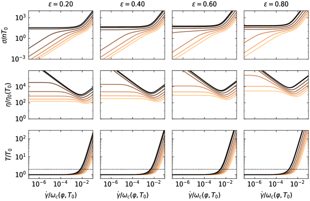
Figure 2: Protocol H (Shear heating increases the granular temperature). For several values of the coefficient of restitution $\varepsilon$ (columns, as indicated) and several packing fractions (color coded) from $\varphi=0.48$ (yellow, bottom) to $\varphi=0.60$ (black, top): (First row) Flow curves, shear stress $\sigma$ as a function of shear rate $\dot{\gamma}$, normalized by the density $n$ and the granular temperature at zero shear, $T_{0}$. (Second row) Viscosity $\eta$ relative to the Boltzmann viscosity $\eta_{0}(T_{0})$, Eq. (66) as a function of shear rate $\dot{\gamma}$. (Third row) Stationary granular temperature $T$, relative to the initial granular temperature, $T_{0}$, at zero shear as a function of shear rate $\dot{\gamma}$. The dotted lines indicate $T/T_{0}\equiv 2$. The shear rate is normalized by the collision frequency $\omega_{c}(\varphi,T_{0})$ of the unsheared system (at granular temperature $T_{0}$) with the prescribed volume fraction.

V.5 Numerical Solutions

The granular mode-coupling equations (63, 64) can in general only be solved numerically. The same applies to the generalized Green-Kubo relation (61). To this end we need the static structure factor and the sound damping constant in the reference state. For the structure factor we resort to the Percus-Yevick expression Percus and Yevick (1958) for elastic hard spheres to be consistent with the discussion of the granular glass transition Kranz et al. (2010, 2013). One could just as well use structure factors from numerical simulations of the reference state, given they are available at sufficient quality. The dependence on the coefficient of restitution manifests itself primarily in the height of the first peak. For the sound damping constant we used the Enskog expression of Garzó and Montanero (2002). It is not a crucial ingredient but more precise values could easily be incorporated. For more technical details on the numerical procedure see appendix E.

VI Results

To obtain quantitative predictions, we numerically solved Eqs. (63, 64, 61) (see Sec. V.5 and appendix E). Some of the results are presented in Ref. Kranz et al. (2018). Here we will focus on a broader range of parameters and provide additional comparison with established kinetic theories.

VI.1 Rheology & Flow Curves

VI.1.1 Protocol H

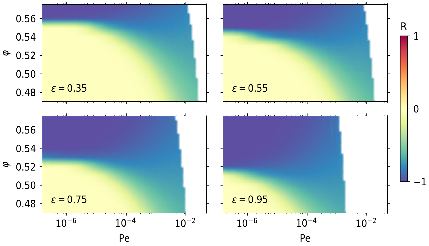
Figure 3: Protocol T ($T\equiv T_{0}$) or Protocol H ($T>T_{0}$): Dynamic state diagrams in the plane spanned by Péclet number, $\operatorname{Pe}$, and packing fraction, $\varphi$, for several values of the coefficient of restitution, $\varepsilon$, as indicated. The effective exponent $R$ quantifying the shear rate dependence of the viscosity, $\eta(\operatorname{Pe})\sim\operatorname{Pe}^{R}$, is color coded on the same scale as in Fig. 1. The inaccessible regime $\operatorname{Pe}>\operatorname{Pe}_{\infty}$ is left blank. The jagged boundary is due to discretization.

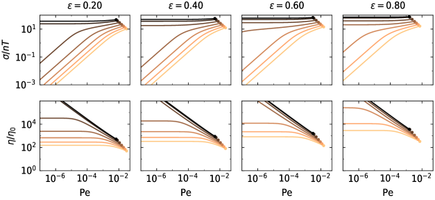
Figure 4: Protocol T ($T\equiv T_{0}$) or Protocol H ($T>T_{0}$): Flow curves, shear stress $\sigma$ as a function of Péclet number $\operatorname{Pe}$ (first row), and viscosity $\eta$ relative to the Boltzmann viscosity $\eta\equiv\eta_{0}(T)$, Eq. (66), (second row) for several values of the coefficient of restitution $\varepsilon$ (columns, as indicated) and several packing fractions (color coded) from $\varphi=0.48$ (yellow, bottom) to $\varphi=0.60$ (black, top). The filled circles mark the maximum Péclet number $\operatorname{Pe}_{\infty}$, i.e., the end of the flow curves for the respective densities.

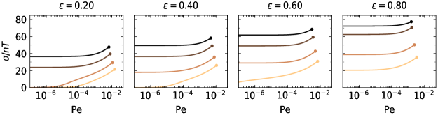
Figure 5: Protocol T ($T\equiv T_{0}$) or Protocol H ($T>T_{0}$): Flow curves, $\sigma(\operatorname{Pe})$, for several values of the coefficient of restitution $\varepsilon$ (as indicated) and several packing fractions (color coded) from $\varphi=0.54$ (yellow, bottom) to $\varphi=0.60$ (black, top) close to and above the glass transition density. Note the linear scale for the shear stress.

The phenomenology of Protocol H has been discussed in Ref. Kranz et al. (2018). Comparing the dynamic state diagrams for different inelasticities, $\varepsilon$, in Fig. 1 confirms the broad layout of the rheological regimes. The critical density for the granular glass transition, $\varphi_{c}(\varepsilon)$, which increases with increasingly dissipative particles determines the boundaries of the Newtonian regime observed at low densities and small shear rates. At the highest shear rates, the power balance, Eq. (4), is dominated by shear heating and shear thickening is observed in the Bagnold regime. As the granular fluid is more susceptible to shear heating the more elastic the particles are, the onset of the Bagnold regime moves to lower shear rates for larger values of $\varepsilon$.

Flow curves, $\sigma(\dot{\gamma})$, corresponding to Protocol H are shown in Fig. 2 (see also Figs. 2 and 3 in Ref. Kranz et al. (2018)). Note that the precise value of the coefficient of restitution may have a comparatively large influence on the flow behavior. For the same flow conditions, i.e., packing fraction, $\varphi$, and shear rate, $\dot{\gamma}$, rather elastic particles may place the granular fluid in the flat part of the flow curve, requiring rather large stresses, $\sigma/nT_{0}\sim 10$, while for more inelastic particles the flow would still be in the Newtonian regime, requiring only negligible shear stress, $\sigma/nT_{0}\ll 1$. This is also reflected in the viscosity (Fig. 2) which may vary over many orders of magnitude for a fixed packing fraction, $\varphi$, depending on both shear rate and coefficient of restitution. A natural scale to compare viscosities to is the Boltzmann viscosity,

$$\eta_{0}:=\eta(\varphi\to 0,\varepsilon=1)=\frac{5}{16d^{2}}\sqrt{T/\pi},$$ (66)

of an elastic hard sphere gas at vanishing density Chapman and Cowling (1970). Fig. 2 shows that viscosities far exceeding this value are predicted at the considered densities. Considering the stationary granular temperature $T$, resulting from the power balance, Eq. (4), we observe that, as expected, significant shear rates are needed to make shear heating relevant and increase the stationary granular temperature, $T$, with respect to the granular temperature $T_{0}$ of the unsheared fluid (Fig. 2). In Ref. Kranz et al. (2018) we defined the critical Péclet number, $\operatorname{Pe}^{*}$, for the onset of shear thickening, as the point where $T=2T_{0}$. Comparing the temperature curves in Fig. 2 with the viscosity curves, $\eta(\dot{\gamma})$, confirms the utility of this definition.

If we normalize the shear stress, $\sigma/nT$, with the stationary granular temperature, $T$, instead of the initial granular temperature, $T_{0}$, and express the shear rate, $\dot{\gamma}$, in terms of the Péclet number, $\operatorname{Pe}$, we arrive at a description of the rheology in terms of intrinsic quantities that make the temperature independence of the (inelastic) hard sphere fluid manifest (Figs. 3,4). In this form, the predictions for Protocol H are identical to the ones for Protocol T as they only differ in the temperature control (cf. Sec. II.1).

VI.1.2 Protocol T

Employing Protocol T makes it straightforward to obtain the intrinsic quantities, $\sigma/nT$, and $\operatorname{Pe}=\dot{\gamma}/\omega_{c}(\varphi,T)$, as the granular temperature is held constant, $T\equiv T_{0}$, throughout. In terms of the packing fraction, $\varphi$, and the Péclet number, $\operatorname{Pe}$, the dynamic state diagram is shown in Fig. 3 for different inelasticities $\varepsilon$. We readily observe that the shear thickening regime vanishes altogether compared to the diagrams for Protocol H (Fig. 1). The apparent shear thickening observed in Protocol H is due to shear heating only, which is absent in Protocol T. As the Péclet number is restricted to be smaller than the maximal value, $\operatorname{Pe}\leq\operatorname{Pe}_{\infty}$ Kranz et al. (2018), the dynamic state diagram includes unreachable regions of large Péclet number, $\operatorname{Pe}>\operatorname{Pe}_{\infty}(\varphi,\varepsilon)$ that cannot be realized in a granular fluid. The Bagnold regime of Protocol H (cf. Fig. 1) shrinks to the line $\operatorname{Pe}=\operatorname{Pe}_{\infty}(\varphi,\varepsilon)$ for Protocol T. At low Péclet number or shear rate, where shear heating is negligible, the dynamic state diagrams become indistinguishable between Protocols H and T (cf. Figs. 1 and 3). Shear thinning behavior, which is caused by the slow relaxation in the fluid Kranz et al. (2018, 2010) is independent of temperature control and is therefore also observed in Protocol T.

The flow curves, $\sigma(\operatorname{Pe})$, for Protocol T shown in Fig. 4 (see also Fig. 2 in Ref. Kranz et al. (2018)) also reflect the finite admissible range of Péclet numbers as they end at $\operatorname{Pe}=\operatorname{Pe}_{\infty}$. The viscosity curves (Fig. 4) confirm that no shear thickening is observed in Protocol T and the Newtonian regime at low densities and small shear rates is complemented by a shear thinning regime only. For packing fractions, $\varphi>\varphi_{c}(\varepsilon)$, above the glass transition, the variation of the shear stress, $\sigma$, with Péclet number, $\operatorname{Pe}$, is remarkably small throughout the whole range of admissible Péclet numbers (Fig. 5). Once the yield stress, $\sigma_{y}=\sigma(\operatorname{Pe}\to 0)$, is exceeded, no more than roughly a doubling of the shear stress will be needed to achieve arbitrary shear rates.

VI.2 Transport Coefficients and Yield Stress

Irrespective of the possibility to handle arbitrary shear rates, gitt (and more generally itt) can also be used to calculate the viscosity, $\eta$, in the linear response regime, $\dot{\gamma}\to 0$. Recall that in this limit Protocol T and H become indistinguishable as there is no shear heating. Employed in this way, gitt extends the low density Enskog predictions Garzó and Montanero (2002), to higher densities (Fig. 6). In particular it captures the strong increase and eventual divergence of the viscosity, $\eta(\varphi)\propto(\varphi_{c}(\varepsilon)-\varphi)^{-\gamma(\varepsilon)}$ with $\gamma(\varepsilon)\sim 2.4$ as the glass transition is approached Kranz et al. (2018, 2013). This divergence can, of course, not be recovered by the low density, Enskog predictions. The variations in the glass transition, $\varphi_{c}(\varepsilon)$, with the coefficient of restitution, $\varepsilon$, leads to a correspondingly large variation of the viscosity, $\eta(\varepsilon)$, which far exceeds the variations predicted by Enskog theory.

The large shear rate behavior, $\dot{\gamma}\to\infty$, or $\operatorname{Pe}\to\operatorname{Pe}_{\infty}$, respectively, is characterized by the Bagnold coefficient $B:=\sigma/{\dot{\gamma}}^{2}$, Fig. 7a. As shear heating is more effective for more elastic particles (in Protocol H), the Bagnold coefficient increases with $\varepsilon$. As the glass is already shear-molten in the Bagnold regime, unlike the viscosity $\eta$, the Bagnold coefficient does not diverge at the glass transition density, $\varphi_{c}(\varepsilon)$. However, the increasing sluggishness of the fluid at high densities is also reflected in the Bagnold coefficient which increases rapidly with density. Such a quick rise is naturally not recovered by the existing Enskog predictions. The theories by Mitarai and Nakanishi (2005), and Kumaran (2006) both come close to the results from gitt for lower densities but deviate by orders of magnitude close to the glass transition density. The simple prediction by Savage and Jeffrey (1981), $B_{\mathrm{SJ}}d=32\varphi\chi(\varphi)/35\pi$, where $\chi(\varphi)$ is the value of the pair correlation function at contact is independent of the coefficient of restitution but also yields the right order of magnitude at low densities.

While the Bagnold coefficient of Savage and Jeffrey (1981) is expressed in terms of the pair correlation function at contact of elastic hard spheres, namely, the Carnahan-Starling approximation Hansen and McDonald (1990) that is very good up to $\varphi\approx 0.4$, Jenkins (2007) later used an empirical, high-density pair-correlation function that diverges at $\varphi_{\mathrm{rcp}}\approx 0.64$ to predict a Bagnold coefficient $B_{J1}$, Eq. (100), that is formally close to Savage and Jeffrey’s expression, but depends on the coefficient of restitution $\varepsilon$ and diverges at $\varphi_{\mathrm{rcp}}$. Note that, as discussed in Ref. Kranz et al. (2018), we underestimate the granular glass transition by roughly $5.5\%$, corresponding to $\Delta\varphi\sim 0.055$ for $\varepsilon=0.6$. To compare Jenkins’ results to ours, we consequently display his result for $B_{J1}(\varphi-0.055)$ in Fig. 7 at a shifted density, so that it now diverges at $\varphi=0.585$. In a later paper, Jenkins and Berzi (2010) put forward the idea of a lower shear jamming density at $\varphi\approx 0.6$ for $\varepsilon\approx 0.7$, implying a divergence of the Bagnold coefficient $B_{J2}$ at $\varphi\approx 0.6$, Eq. (104). Again shifting density for comparison with our results, we show $B_{J2}(\varepsilon=0.6,\varphi-0.055)$ in Fig. 7a.

In contrast, the granular mode-coupling theory here applies to a driven granular fluid and predicts a granular glass transition and the emergence of a yield stress at a critical density $\varphi_{c}(\varepsilon)<\varphi_{\mathrm{rcp}}$. The discussion of the relevant time scales Kranz et al. (2018) and the dynamic state diagrams, cf. Fig. 1 shows that the shear rate in the Bagnold regime, $\dot{\gamma}_{\infty}$, exceeds the structural relaxation rate, $\tau_{\alpha}^{-1}$. Therefore, the slow relaxation, $\tau_{\alpha}\to\infty$ indicating the granular glass transition, is irrelevant for the Bagnold regime and the Bagnold coefficient must be smooth across the granular glass transition. This is, indeed, the case for the Bagnold coefficient $B$ calculated by the gitt formalism (Fig. 7a).

Above the glass transition density, $\varphi_{c}(\varepsilon)$, a finite (dynamic) yield stress, $\sigma_{y}$, has to be exceeded to keep the system flowing and to prevent it from freezing into an amorphous glass. The critical yield stress, $\sigma_{y}^{c}(\varepsilon)$ (cf. Fig. 3 in Ref. Kranz et al. (2018)) right at the glass transition is on the order of $6$–$9nT$. For larger densities, $\varphi>\varphi_{c}(\varepsilon)$, the yield stress quickly rises with density (Fig. 7b) as expected .

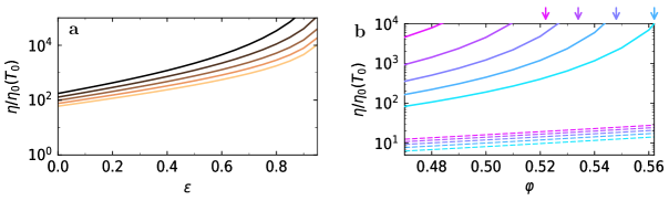
Figure 6: Viscosity $\eta$, normalized by the Boltzmann viscosity $\eta_{0}$, Eq. (66), at small shear rate, $\dot{\gamma}\to 0$. (a) As a function of the coefficient of restitution $\varepsilon$ for a number of packing fractions from $\varphi=0.47$ (yellow, bottom) to $\varphi=0.51$ (black, top). (b) As a function of packing fraction, $\varphi$, for a number of values of the coefficient of restitution, $\varepsilon$, from $\varepsilon=0.1$ (cyan, bottom) to $\varepsilon=0.9$ (magenta, top). Solid lines denote gitt predictions while dashed lines indicate the Enskog low density expansion by Garzó and Montanero (2002). The arrows indicate the glass transition density, $\varphi_{c}(\varepsilon)$.

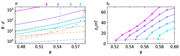
Figure 7: (a) Bagnold coefficient $B$ as a function of packing fraction $\varphi$. Solid lines are gitt predictions for a number of values of the coefficient of restitution, $\varepsilon$, from $\varepsilon=0.1$ (cyan, bottom) to $\varepsilon=0.9$ (magenta, top). The dashed lines denote Enskog predictions from Savage and Jeffrey (1981) (blue), Kumaran (2006) (orange), and Mitarai and Nakanishi (2005) (green). The last two are for $\varepsilon=0.9$. The arrows indicate the glass transition density, $\varphi_{c}(\varepsilon)$. The dot-dashed lines are the predictions by Jenkins et al. Jenkins and Berzi (2010); Jenkins (2007) $B_{J1}$ (red) and $B_{J2}$ (violet) for $\varepsilon=0.6$ (cf. appendix F). (b) Yield stress, $\sigma_{y}$, as a function of volume fraction, $\varphi$, for a number of values of the coefficient of restitution, $\varepsilon$, from $\varepsilon=0.9$ (magenta, left) to $\varepsilon=0.1$ (cyan, right). Points are calculated and lines are a guide to the eye. The dotted horizontal line indicates the critical yield stress $\sigma_{y}^{c}$ at the granular glass transition.

VII Conclusion

In summary, we have shown how to derive generalized Green-Kubo relations, Eq. (30), for sheared frictionless inelastic hard sphere fluids at finite shear rates and densities around the (granular) glass transition density. In particular, we have shown that an itt formalism can be derived for a granular fluid which is generically out of euilibrium, even in the absence of shear. Here, we focused on the generalized Green-Kubo relation for the shear stress $\sigma$, Eq. (33), that we found to be formally identical to the one for thermalized colloidal suspensions, Eq. (37) in Ref. Fuchs and Cates (2009), but for the prefactor $(1+\varepsilon)/2$. The starting point was the exact relation (8), expressing the phase space distribution of the sheared stationary state, $\varrho_{\mathrm{ss}}$, in terms of the distribution of the quiescent but out-of-equilibrium reference state, $\varrho_{\mathrm{ref}}$. The essential approximations were: (i) the assumption that the microscopic shear stress captures the change of $\varrho_{\mathrm{ref}}$ due to shear, Eq. (9), and (ii) to replace the decay of stress correlations under the Green-Kubo integral by the slow relaxation of density fluctuations encoded in the transient correlator $\Phi_{\bm{q}}(t)$, Eq. (12). The coupling constants, Eq. (32), capture the essential shear induced anisotropy making it sufficient to consider an isotropic transient correlator $\Phi_{q}(t)$, Eq. (61). The derivation showed that the generalized Green-Kubo relation (12) is neither restricted to small shear rates, $\dot{\gamma}\to 0$, nor to quasi-elastic particles, $\varepsilon\to 1$. To ensure a clear separation of time scales between the slow relaxation of density fluctuations and all other relaxation modes in the fluid, the density needs to be not too far below the granular glass transition density $\varphi_{c}(\varepsilon)$ Kranz et al. (2010). On the upper end, it should be sufficiently far away from the random close packing density, $\varphi_{\mathrm{rcp}}\approx 0.64$, as we do not take the jamming transition into account. Coveniently, details of the driving mechanism do no longer feature explicitly in the generalized Green-Kubo relation (12).

For a homogeneously cooling granular gas, a Green-Kubo relation akin to Eq. (10) has been developed by Goldhirsch and van Noije (2000) following Ronis’ Ronis (1979) perturbative approach but they have kept the stress auto-correlation function as an irreducible function. Kumaran (2009b) has derived a Green-Kubo relation similar to our result, Eq. (12), for a dilute quasi-elastic sheared granular gas in the Bagnold regime. His result is perturbative in the small parameter $\sqrt{1-\varepsilon}$. While it incorporates wave vector advection and employs a factorization of the time evolution operator similar to our mode-coupling approximation, it uses the linearized granular hydrodynamic equations valid at low density and small wave number, $kd\ll 1$.

To capture the slow glassy relaxation in the quiescent fluid that is a result of strongly correlated dynamics and sensitive to local particle configurations, $kd\gtrsim 1$ Debenedetti and Stillinger (2001); Kranz et al. (2013), we had to go beyond linearized hydrodynamic equations. Instead, we derived a set of non-linear, generalized hydrodynamic equations for the transient correlator, Eqs. (51,57), explicitly taking into account the shear advection of wave vectors and the loss of detailed balance due to the inelastic collisions. The latter is manifest in the modified speed of sound, Eq. (49), and the two unequal coupling constants in the memory kernel, $\mathcal{V}^{\lambda}_{\bm{q}\bm{k}\bm{p}},\mathcal{W}^{\lambda}_{\bm{q}\bm{k}\bm{p}}$, Eqs. (59), see also Refs. Kranz et al. (2010, 2013). To this end, we kept the exact inelastic binary collision operator, Eq. (16), but approximated the non-equilibrium phase space distribution $\varrho_{\mathrm{ref}}$ of the reference fluid as essentially the canonical distribution of an elastic hard sphere fluid (cf. Sec. II.1). Let us once more stress that here the essential approximation is the factorization between spatial and velocity degrees of freedom. A quantitative understanding of these correlations is currently lacking and numerical results are limited to the low density, two-dimensional data of Pagonabarraga et al. (2001). A fully quantitative treatment of the coupling between relative positions and velocities is therefore currently out of reach. However, in order to assess the validity of our approximations, let us sketch the qualitative influence of these correlations on the gitt formalism. As the correlations are short ranged Pagonabarraga et al. (2001), we expect them to primarily affect the collision integrals used to calculate the vertices. In effect, the mean collisional force is reduced through the depletion of head-on collisions. This has two counteracting effects: (i) It reduces the shear stress at a given density, but (ii) it shifts the granular glass transition to higher densities. In conclusion, we expect the shear stress at a given distance from the granular glass transition to be only weakly dependent on the coupling between positions and velocities. Non-Gaussian corrections to the velocity distribution as well as structure factors that characterize the actual granular fluid could be incorporated in extensions of our work.

A notable feature of the gitt approach presented here is that it associates the emergence of a yield stress with the dynamic granular glass transition. The corresponding glass transition densities, $0.52\lesssim\hat{\varphi}_{c}(\varepsilon)\lesssim 0.6$ Kranz et al. (2010, 2018), are lower than the eventual jamming density at $\varphi_{\mathrm{rcp}}\approx 0.64$. In essence, we predict the emergence of a yield stress (characterizing a quiescent amorphous solid) without lasting contacts between the particles. Shear thinning is then associated with the shear rate $\dot{\gamma}$ exceeding the structural relaxation rate of the granular fluid Kranz et al. (2018). The latter is a hallmark of glassy behavior but is at variance with alternative approaches to granular rheology that attribute the yielding transition at densities below $\varphi_{\mathrm{rcp}}$ with the shear induced emergence of lasting contacts Reddy and Kumaran (2007); Kumaran (2009c, a, 2014); Jenkins and Berzi (2010), i.e., a divergence of the pair correlation function at contact, $\chi$. Resolving which of the mechanisms controls the physics, requires, we believe, additional experiments and simulations.

The increase of the shear stress at high densities is driven by the slow structural relaxation of the system around the glass transition. The dependence of the glass transition on the coefficient of restitution yields a strong sensitivity of the transport coefficients and even the qualitative rheological behavior on the inelasticity of the particles. This sensitivity, together with the strong increase (and eventual divergence) of the small shear viscosity, $\eta(\dot{\gamma}\to 0)$, shows that an extrapolation of the Enskog predictions from the gaseous state of vanishing density, $\varphi\ll 1$, to significant densities, $\varphi\sim\mathcal{O}(1)$, cannot work as it completely neglects the dramatic slowing down of structural relaxation at high densities. For the Bagnold coefficient, $B$, we have argued that it is only defined for finite shear rates, $\dot{\gamma}_{\infty}=\omega_{c}\operatorname{Pe}_{\infty}$. Except for the elastic limit, $\varepsilon\to 1$, where $\operatorname{Pe}_{\infty}\ll 1$, this makes the Bagnold coefficient inaccessible to linear response theories but places it well within the reach of gitt.

The hard-sphere property that the temperature, $T$, only enters as a timescale via the collision frequency, $\omega_{c}\sim\sqrt{T}$, and does not control the physics, is retained by gitt. In terms of the Péclet number, $\operatorname{Pe}$, and the dimensionless shear stress $\sigma/nT$, the theory is manifestly temperature independent. The choice of temperature control in an experiment, however, has a profound influence on the phenomenology observed. If shear heating is not compensated (Protocol H), the work expended on heating the system will manifest as an apparent shear thickening (Fig. 1). However, the viscosity $\eta\sim\sqrt{T}$ trivially rises with temperature and if we take this into account (Fig. 3), no shear thickening remains. Dialing down the random driving force we can keep the temperature constant (Protocol T), However, this only works below a maximal shear rate, $\dot{\gamma}\leq\omega_{c}\operatorname{Pe}_{\infty}$. For higher shear rates even switching off the random driving completely cannot compensate shear heating.

We have focused here on the derivation of gitt and only discussed the most fundamental predictions of the theory. The experience from the rheology of colloidal suspensions shows that the itt formalism can contribute to the description of a much broader range of phenomena. We are planning to explore these in future work. Straightforward extensions include a more realistic, velocity dependent coefficient of restitution Schwager and Pöschel (2008). We do not expect such a refined model to qualitatively change our results. On the other hand, the rheology of granaular fluids is strongly effected Grob et al. (2014, 2016); Wyart and Cates (2014) by frictional interactions of the grains, which could be taken into account by tangential restitution and Coulomb friction as in Refs. Herbst et al. (2000, 2005). Another extension are larger size disparities, which may entail new phenomena Imhof and Dhont (1995) and are left for subsequent studies. Our formalism could also be extended to treat non-spherical particles Aspelmeier et al. (2001), albeit at the expense of a further increase in technical complexity. A necessary first step would be to promote the understanding of the orientational Schilling and Scheidsteger (1997); Theenhaus et al. (2001); Chong and Götze (2002); Elizondo-Aguilera et al. (2014) glass transition to the granular realm. Tackling this formidable task is far beyond the scope of the present study and shall be left to future work. In the present work, we have neglected drag forces and hydrodynamic interactions induced by a possible interstitial fluid and effectively consider particles in vacuum, leaving a discussion of two-phase flow effects to future work.

Appendix A The Sllod Equations of Motion

The Sllod equations form the basis of the work presented here. As they posses some non-intuitive features and have been a matter of debate in the literature Evans and Morriss (1990); Edwards and Dressler (2001); Edwards et al. (2006); Daivis and Todd (2006), we will sketch their derivation. To make contact with the literature, let’s assume for the moment that particles interact via smooth pair potentials $V(r_{ij})$. Then the Hamiltonian of the system is generically given as $H(\bm{r}_{1},\ldots,\bm{r}_{N},\bm{v}_{1},\ldots,\bm{v}_{N})=\sum_{i}v_{i}^{2}/2+\sum_{i<j}V(r_{ij})$.

To single out the imposed flow profile $\bm{u}(\bm{r})=\bm{r}\cdot\mathsf{k}$, we make the non-canonical transformation $\bm{v}_{i}\to\bm{c}_{i}=\bm{v}_{i}-\bm{r}_{i}\cdot\mathsf{k}$. In the new coordinates the Hamiltonian

$$H_{\mathrm{nc}}(\bm{r}_{1},\ldots,\bm{r}_{N},\bm{c}_{1},\ldots,\bm{c}_{N})=\sum_{i}\left(\frac{1}{2}c_{i}^{2}+\bm{r}_{i}\bm{c}_{i}:\mathsf{k}\right)+\tilde{V}(\bm{r}_{1},\ldots,\bm{r}_{N})$$ (67)

assumes the form of a Dolls-Hamiltonian, albeit with a a modified effective potential $\tilde{V}(\bm{r}_{1},\ldots,\bm{r}_{N}):=\sum_{i<j}V(r_{ij})+\frac{1}{2}\sum_{i}(\bm{r}_{i}\cdot\mathsf{k})^{2}$ Edwards and Dressler (2001). The canonical Hamilton equations no longer hold for the non-canonical Hamiltonian, Eq.(67), expressed in non-canonical coordinates. Instead, the same transformation has to be applied to the canonical Poisson brackets, $\{\cdot,\cdot\}\to\{\cdot,\cdot\}_{\mathrm{nc}}$ (Eq. (22) in Edwards and Dressler, 2001). The resulting equations of motion are the Sllod equations

$$\dot{\bm{r}}_{i} =\{\bm{r}_{i},H_{\mathrm{nc}}\}_{\mathrm{nc}}=\bm{c}_{i}+\bm{r}_{i}\cdot\mathsf{k}$$ (68)

$$\dot{\bm{c}}_{i} =\{\bm{c}_{i},H_{\mathrm{nc}}\}_{\mathrm{nc}}=\bm{F}_{i}-\bm{c}_{i}\cdot\mathsf{k}-\bm{r}_{i}\cdot\mathsf{k}\cdot\mathsf{k}$$ (69)

where $\bm{F}_{i}:=-\sum_{j\neq i}\nabla V(r_{ij})$ is the total force on particle $i$.

Note that the net forces are not independent of the flow profile. Indeed one can show that the time averaged force $\overline{\bm{F}}(\bm{r}):=\overline{\sum_{i\in O}\bm{F}_{i}}$ acting on a fluid element $O$ at position $\bm{r}$ is fully determined by the velocity gradient tensor, $\overline{\bm{F}}(\bm{r})=\bm{r}\cdot\mathsf{k}\cdot\mathsf{k}$ Edwards et al. (2006). Therefore any fluctuations $\delta\bm{u}(\bm{r}):=\bm{u}(\bm{r})-\bm{r}\cdot\mathsf{k}=\sum_{i\in O}\bm{c}_{i}$ follow the simple equation of motion

$$\delta\dot{\bm{u}}(\bm{r},t)=-\delta\bm{u}(\bm{r},t)\cdot\mathsf{k}+\delta\bm{F}(\bm{r},t)$$ (70)

where $\delta\bm{F}(\bm{r},t)=\bm{F}(\bm{r},t)-\overline{\bm{F}}(\bm{r})$ is the fluctuating force. The first term on the right hand side of Eq. (70) is problematic. Depending on the velocity gradient tensor $\mathsf{k}$ it may lead to unbounded growth of a spontaneous fluctuation $\delta\bm{u}(\bm{r},0)$. In simulations this is avoided by taking the whole simulation volume as the fluid element $O$ and using deterministic boundary forces (e.g., Lees-Edwards boundary conditions) with vanishing fluctuations $\delta\bm{F}=\bm{0}$. Together with a perfect initial flow field, $\delta\bm{u}(\bm{r},t=0)=\bm{0}$, this keeps the fluctuations in the flow field at exactly zero for all times as the total momentum of the system

$$\sum_{i}\bm{c}_{i}(0)=\bm{0}$$ (71)

is conserved.

For interacting particles, one expects viscous heating, i.e., the transfer of energy from the flow field $\bm{r}\cdot\mathsf{k}$ to the internal energy $E_{\mathrm{int}}:=\sum_{i}c_{i}^{2}/2+\sum_{i<j}V(r_{ij})\neq H_{\mathrm{nc}}$. Indeed, one finds

$$\frac{dE_{\mathrm{int}}}{dt}=-\sigma:\mathsf{k}-\dot{W}_{\mathrm{exp}}$$ (72)

where $W_{\mathrm{exp}}=\sum_{i}\bm{r}_{i}\bm{c}_{i}:\mathsf{k}\cdot\mathsf{k}$ is the work performed by the fluid due to an expansive flow field Edwards et al. (2006). As it is usually desired to keep the temperature—related to the internal energy—of the fluid constant, a thermostat has to be employed Evans and Morriss (1990). In the present work we are solely concerned with linear shear flows where $\nabla\bm{u}\cdot\nabla\bm{u}\equiv 0$. simplifying both Eqs. (69) and (72).

Appendix B The Density-Stress-Overlap for Hard Spheres

To make contact with established results, it is instructive to recall the origin of the momentum current tensor $\mathsf{P}$ in the continuity equation for momentum

$$\partial_{t}\bm{j}(\bm{r},t)\equiv i\mathcal{L}^{+}_{\mathrm{ref}}\bm{j}(\bm{r},t)=-\nabla\cdot\mathsf{P}(\bm{r},t).$$ (73)

In reciprocal space we therefore have Wajnryb et al. (1995)

$$-i\bm{q}\cdot\mathsf{P}(\bm{q})=i\bm{q}\cdot\frac{\bm{\hat{q}}\bm{\hat{q}}}{iq}i\mathcal{L}_{0}j_{\bm{q}}^{L}+i\bm{q}\cdot\sum_{j<k}\frac{\bm{\hat{r}}_{jk}}{i\bm{q}\cdot\bm{\hat{r}}_{jk}}i\mathcal{T}^{+}_{jk}\bm{j}_{\bm{q}},$$ (74)

where $j_{\bm{q}}^{L}=\bm{\hat{q}}\cdot\bm{j}_{\bm{q}}$ is the longitudinal current. In the absence of macroscopic flows ($\bm{u}\equiv\bm{0}$) such that $\sigma_{\alpha\beta}\equiv-P_{\alpha\beta}$ and in the homogeneous limit $\bm{q}\to 0$ this indeed recovers the Irving-Kirkwood expressions $\sigma_{\alpha\beta}^{\mathrm{kin}}(\bm{q}\to 0)=\sum_{j}v_{j}^{\alpha}v_{j}^{\beta}$, and

$$\sigma_{\alpha\beta}^{\mathrm{int}}(\bm{q}\to 0) =-\frac{1+\varepsilon}{2}\sum_{j<k}\frac{\hat{r}_{jk}^{\alpha}\hat{r}_{jk}^{\beta}}{i\bm{q}\cdot\bm{\hat{r}}_{jk}}(\bm{\hat{r}}_{jk}\cdot\bm{v}_{jk})^{2}\theta(-\bm{\hat{r}}_{jk}\cdot\bm{v}_{jk})\delta(r_{jk}-d)\left(e^{i\bm{q}\cdot\bm{r}_{k}}-e^{i\bm{q}\cdot\bm{r}_{j}}\right)$$ (75)

$$=\frac{1+\varepsilon}{2}\sum_{j<k}\frac{i\bm{q}\cdot\bm{r}_{jk}}{i\bm{q}\cdot\bm{\hat{r}}_{jk}}\hat{r}_{jk}^{\alpha}\hat{r}_{jk}^{\beta}(\bm{\hat{r}}_{jk}\cdot\bm{v}_{jk})^{2}\theta(-\bm{\hat{r}}_{jk}\cdot\bm{v}_{jk})\delta(r_{jk}-d)$$ (76)

$$=\frac{1+\varepsilon}{2}d\sum_{j<k}\hat{r}_{jk}^{\alpha}\hat{r}_{jk}^{\beta}(\bm{\hat{r}}_{jk}\cdot\bm{v}_{jk})^{2}\theta(-\bm{\hat{r}}_{jk}\cdot\bm{v}_{jk})\delta(r_{jk}-d),$$ (77)

independent of $\bm{\hat{q}}$ Dufty (2012); Baskaran et al. (2008). The vertex $\mathsf{A}:=-\left\langle\rho_{\bm{k}}\rho_{-\bm{k}}\mid\mathcal{Q}\mathsf{P}(\bm{q}=\bm{0})\right\rangle=\bm{\hat{k}}\bm{\hat{k}}A_{\parallel}+(\mathsf{1}-\bm{\hat{k}}\bm{\hat{k}})A_{\perp}$ may be split into a longitudinal and a transverse part

$$A_{\parallel}=\bm{\hat{k}}\bm{\hat{k}}:\mathsf{A},\quad\text{and}\quad A_{\perp}=\bm{\hat{k}}^{\perp}\bm{\hat{k}}^{\perp}:\mathsf{A},\quad\text{and}\quad$$ (78)

where $\bm{\hat{k}}^{\perp}\perp\bm{\hat{k}}$. Then the off-diagonal component is given by $A_{xy}=\bm{\hat{k}}_{x}\bm{\hat{k}}_{y}(A_{\parallel}-A_{\perp})$.

In order to calculate the expectation values $A_{\parallel}$ and $A_{\perp}$, we start with the stress tensor at finite $\bm{q}$ and only perform the limit $q\to 0$ in the end. For $A_{\parallel}$ momentum conservation enforces $\bm{q}\parallel\bm{k}$ such that

$$A_{\parallel}=-\lim_{q\to 0}\left\langle\rho_{\bm{k}}\rho_{q\bm{\hat{k}}-\bm{k}}\mid\mathcal{Q}\bm{\hat{k}}\bm{\hat{k}}:\mathsf{P}(q\bm{\hat{k}})\right\rangle$$ (79)

where

$$-\bm{\hat{k}}\bm{\hat{k}}:\mathsf{P}(q\bm{\hat{k}})=\frac{1}{iq}i\mathcal{L}_{0}j_{q\bm{\hat{k}}}^{L}+\sum_{j<k}\frac{\bm{\hat{k}}\cdot\bm{r}_{jk}}{iq\bm{\hat{k}}\cdot\bm{r}_{jk}}i\mathcal{T}^{+}_{jk}j_{q\bm{\hat{k}}}^{L}=\frac{1}{iq}i\mathcal{L}^{+}_{\mathrm{ref}}j_{q\bm{\hat{k}}}^{L},$$ (80)

i.e.,

$$A_{\parallel}=\lim_{q\to 0}\frac{1}{iq}\left\langle\rho_{\bm{k}}\rho_{q\bm{\hat{k}}-\bm{k}}\mid\mathcal{Q}i\mathcal{L}^{+}_{\mathrm{ref}}j_{q\bm{\hat{k}}}^{L}\right\rangle.$$ (81)

With the same line of argument we arrive at

$$A_{\perp}=-\lim_{q\to 0}\left\langle\rho_{\bm{k}}\rho_{q\bm{\hat{k}}^{\perp}-\bm{k}}\mid\mathcal{Q}\bm{\hat{k}}^{\perp}\bm{\hat{k}}^{\perp}:\mathsf{P}(q\bm{\hat{k}}^{\perp})\right\rangle=-\lim_{q\to 0}\frac{1}{iq}\left\langle\rho_{\bm{k}}\rho_{q\bm{\hat{k}}^{\perp}-\bm{k}}\mid\mathcal{Q}i\mathcal{L}^{+}_{\mathrm{ref}}j_{q\bm{\hat{k}}^{\perp}}^{L}\right\rangle.$$ (82)

From the literature Kranz et al. (2013) we know

$$\left\langle\rho_{\bm{k}}\rho_{\bm{q}-\bm{k}}\mid\mathcal{Q}i\mathcal{L}^{+}_{\mathrm{ref}}j_{\bm{q}}^{L}\right\rangle=\frac{1+\varepsilon}{2}iT\left[(\bm{\hat{q}}\cdot\bm{k})S_{|\bm{q}-\bm{k}|}+\bm{\hat{q}}\cdot(\bm{q}-\bm{k})S_{k}-qS^{(3)}(\bm{k},\bm{q}-\bm{k})/S_{q}\right],$$ (83)

where $S^{(3)}(\bm{k},\bm{p})$ is the triplet static structure factor Rosenfeld et al. (1990). The magnitude of the off-diagonal term can therefore be calculated as

$$A_{\parallel}-A_{\perp} =\frac{1+\varepsilon}{2}T\lim_{q\to 0}\left[k\frac{S_{k-q}-S_{k}}{q}+S_{k}-\frac{S^{(3)}(\bm{k},q\bm{\hat{k}}-\bm{k})}{S_{q}}-S_{k}+\frac{S^{(3)}(\bm{k},q\bm{\hat{k}}^{\perp}-\bm{k})}{S_{q}}\right]$$ (84)

$$=-\frac{1+\varepsilon}{2}TkS^{\prime}_{k}$$

employing the geometric relations between $\bm{q}$ and $\bm{k}$ and using that $S(q\to 0)\neq 0$. The latter is true for both elastic and dissipative hard sphere fluids in the stationary state but fails in hyperuniform configurations Torquato (2018). For elastic spheres ($\varepsilon=1$) this constitutes a kinetic derivation of the stress-density overlap that has previously been derived from thermodynamic arguments Fuchs and Cates (2009).

Appendix C The Case of Viscous Dissipation

Besides modeling granular particles as hard spheres with a coefficient of restitution $\varepsilon$, an often used and equally valid approach is to model them as soft spheres with a finite ranged, elastic repulsive force $\bm{F}_{i}^{\mathrm{el}}(r_{ij})$ Pöschel and Schwager (2005). In this case, dissipation is modeled by a viscous force

$$\bm{F}_{i}^{\mathrm{visc}}=-\zeta\sum_{j\neq i}\Theta(d-r_{ij})\bm{\hat{r}}_{ij}(\bm{v}_{ij}\cdot\bm{\hat{r}}_{ij})$$ (85)

acting while the particles are in contact and parameterized by the viscosity $\zeta$, a material property of the particles. Note that $\bm{F}_{i}^{\mathrm{visc}}$ is linear in the relative velocity.

A Liouville operator corresponding to $\bm{F}_{i}^{\mathrm{visc}}$ is easily constructed, $i\mathcal{L}^{\mathrm{visc}}=\sum_{i}\bm{F}_{i}^{\mathrm{visc}}\cdot\partial_{\bm{v}_{i}}$. If this Liouville operator is used in Eqs. (81) and (82) above, it can be seen that the viscous contributions vanish due to parity. With this, and in contrast to our expression (12), the generalized Green-Kubo relation for soft granular particles with viscous dissipation does not contain any explicit reference to the dissipative interactions. In fact, it is identical to the relation for purely elastic particles. For the same reason, also the equation of motion for the transient correlator $\Phi_{\bm{k}}(t)$ including its memory kernel in mode-coupling approximation does not contain any term that stems from the viscous dissipation. The only change in the constitutive relation between purely elastic soft particles and dissipative soft particles would then be contained in the change of static structure, $S_{k}$, and is expected to be very weak.

To remedy this unsatisfactory state, Suzuki and Hayakawa (2014) amended the mode-coupling approximation of the stress auto-correlation function, Eq. (10), by a second projection on density-current pairs $\rho_{\bm{k}}\bm{j}_{-\bm{k}}$. These have a finite overlap with the viscous stress $i\mathcal{L}^{\mathrm{visc}}\bm{j}_{\bm{k}}$. However, this forces the introduction of a second, independent transient correlator, $\overline{\bm{H}}_{\bm{k}}(t):=iN\left\langle\bm{j}_{\bm{k}}\mid\rho_{\bm{k}(t)}(t)\right\rangle$ in our notation. Even in the isotropic approximation, $\overline{\bm{H}}_{\bm{k}}(t)$ cannot be reduced to the transient density correlator due to the broken time-reversal symmetry. The second correlator, coming with its own equation of motion coupled to the equation of motion of $\Phi_{\bm{k}}(t)$, substantially increases the complexity of the problem. Although Suzuki and Hayakawa (2014) have shown that it is still manageable, it is not completely clear that to single out density-current pairs is physically consistent. Density-density pairs are unique in that the (transient) correlator is expected to become exceedingly slow compared to microscopic time scales close to the glass transition. Currents, however, do not freeze at the glass transition and current correlations are expected to decay rapidly. At this point, it is not obvious if there are other decay channels in addition to $\overline{\bm{H}}_{\bm{k}}(t)$ that would be equally important and would have to be included.

Appendix D The Directional Average of Eq. (52)

The following derivation is standard in the itt literature Fuchs and Cates (2009); Chong and Kim (2009); Suzuki and Hayakawa (2013) but we include it here for the sake of completeness. The vector valued density-current correlator $\bm{H}_{\bm{q}}(t)=\bm{\hat{q}}(t)H^{\parallel}_{\bm{q}}(t)+\bm{\hat{q}}^{\perp}(t)H^{\perp}_{\bm{q}}(t)$ has a longitudinal and a transverse component. Here $\bm{\hat{q}}^{\perp}(t)\perp\bm{\hat{q}}(t)$ is an a priori arbitrary unit vector perpendicular to $\bm{\hat{q}}(t)$. From Eq. (62) we have $H_{q}^{\parallel}(t)=S_{q}\dot{\Phi}_{q}(t)/q(t)$; furthermore $\bm{L}_{\bm{q}}=0$ in mode-coupling approximation, so that substitution of Eq. (51b) into Eq. (52) yields

$$S_{q}\ddot{\Phi}_{\bm{q}}(t)+q^{2}(t)C^{2}_{\bm{q}(t)}S_{q}\Phi_{\bm{q}}(t)+q(t)\nu_{\bm{q}(t)}H_{\bm{q}}^{\parallel}(t)+\bm{q}(t)\cdot\int_{0}^{t}d\tau\bm{H}_{\bm{q}}(\tau)\cdot\mathsf{M}_{\bm{q}}(t,\tau)\\ +2\bm{q}(t)\cdot\mathsf{k}\cdot\bm{H}_{\bm{q}}(t)=0.$$ (86)

Once we also split the memory kernel into longitudinal and transverse components

$$\mathsf{M}_{\bm{q}}(t,\tau)=\bm{\hat{q}}(t)\bm{\hat{q}}(t)m_{\bm{q}}^{\parallel}(t,\tau)+[\mathsf{1}-\bm{\hat{q}}(t)\bm{\hat{q}}(t)]m_{\bm{q}}^{\perp}(t,\tau)$$ (87)

we have

$$\bm{q}(t)\cdot[\bm{H}_{\bm{q}}(\tau)\cdot\mathsf{M}_{\bm{q}}(t,\tau)]=q(t)H_{\bm{q}}^{\parallel}(\tau)m_{\bm{q}}^{\parallel}(t,\tau).$$ (88)

We immediately have

$$\bm{q}(t)\cdot\mathsf{k}\cdot\bm{\hat{q}}(t)=\dot{\gamma}q_{x}(t)q_{y}(t)/q(t)$$ (89)

and choose $\bm{q}^{\perp}(t)=\bm{q}(t)\times[\bm{q}(t)\cdot\mathsf{k}]$ perpendicular to $\bm{q}(t)$ and $\bm{q}(t)\cdot\mathsf{k}$. Then

$$\bm{q}(t)\cdot\mathsf{k}\cdot\bm{\hat{q}}^{\perp}(t)=0$$ (90)

and using Eqs. (88, 89, 90), Eq. (86) turns into

$$\ddot{\Phi}_{\bm{q}}(t)+\nu_{\bm{q}(t)}\dot{\Phi}_{\bm{q}}(t)+q^{2}(t)C^{2}_{\bm{q}(t)}\Phi_{\bm{q}}(t)+\int_{0}^{t}d\tau m^{\parallel}_{\bm{q}}(t,\tau)\dot{\Phi}_{\bm{q}}(\tau)+2\dot{\gamma}\frac{q_{x}(t)q_{y}(t)}{q^{2}(t)}\dot{\Phi}_{\bm{q}}(t)=0,$$ (91)

independent of $H_{\bm{q}}^{\perp}(t)$. Averaging Eq. (91) over the directions of $\bm{\hat{q}}(t)$, the last term vanishes and we arrive at Eq. (63). Here we identify $m_{\bm{q}}(t,\tau)\equiv m_{\bm{q}}^{\parallel}(t,\tau)/q^{2}(t)C_{q(t)}^{2}$.

By the same line of arguments, we arrive at the equation of motion for the transverse density-current correlator

$$\frac{d}{dt}H_{\bm{q}}^{\perp}(t)+[\mu_{\bm{q}(t)}-\nu_{\bm{q}(t)}]H_{\bm{q}}^{\perp}(t)+\int_{0}^{t}d\tau m_{\bm{q}}^{\perp}(t,\tau)H_{\bm{q}}^{\perp}(\tau)=0.$$ (92)

Note that it is implicitly coupled to $\Phi_{\bm{q}}(t)$ through the memory kernel.

Appendix E Numerics

In order to solve Eqs. (61, 63, 64) numerically, we adapted an established code Fuchs and Cates (2002). The temperature independence of the hard sphere equations is exploited and the explicit dependence on the coefficient of restitution has been added. For the structure factor, we use the Percus-Yevick Percus and Yevick (1958) explicit solution for hard spheres Ashcroft and Lekner (1966) and for the value of the pair correlation function at contact, $\chi$, we use the Woodcock equation of state WC1 Bannerman et al. (2010). The collision frequency is then given as the elastic Enskog expression, $\omega_{c}(\varphi,T)\simeq 24\varphi\chi d^{-1}\sqrt{T/\pi}$ Hansen and McDonald (1990). For simplicity, instead of calculating $\sigma$ directly, we determine the temperature independent quantity

$$\check{\eta}(\operatorname{Pe},\varphi,\varepsilon):=\frac{1+\varepsilon}{2}\int_{0}^{\infty}\frac{dt^{*}}{\sqrt{1+(\operatorname{Pe}t^{*})^{2}/3}}\int_{0}^{\infty}\frac{dk^{*}{k^{*}}^{4}}{60\pi^{2}}\times\frac{S^{\prime}_{\overline{k}^{*}(-t^{*})}S^{\prime}_{k^{*}}}{S_{k^{*}}^{2}}\Phi^{2}_{\overline{k}(-t^{*})}(t^{*}).$$ (93)

From this result, the quantities of interest can be obtained as

$$\frac{\sigma}{nT}=\frac{\pi}{6}\check{\eta}\frac{\operatorname{Pe}}{\varphi},\quad\frac{\eta}{\eta_{0}(T)}=\frac{2\pi}{15\varphi\chi}\check{\eta},\quad Bd=\frac{\pi}{576}\times\frac{\check{\eta}}{(\varphi\chi)^{2}\operatorname{Pe}}.$$ (94)

As $\eta_{0}\propto\sqrt{T}$, we can derive $\eta/\eta_{0}(T_{0})=\sqrt{T/T_{0}}\times\eta/\eta_{0}(T)$ and in the same manner $\dot{\gamma}/\omega_{c}(T_{0})=\operatorname{Pe}\sqrt{T/T_{0}}$.

The Enskog term, $\nu_{q}$ Eq. (54), is known to drastically underestimate sound damping at high densities. To this end we replace it,

$$\nu_{q}\to\frac{20}{3}\times\frac{D_{S}}{d^{2}}[1+3j^{\prime\prime}_{0}(qd)],$$ (95)

where we chose the Enskog expression for the sound damping constant $D_{S}$ Garzó and Montanero (2002) and note that this expression has the correct hydrodynamic limit, $2D_{S}q^{2}$ for $q\to 0$.

For the wave number integrals, the wave numbers are discretized uniformly at 100 points between $k^{*}=0.4$ and $k^{*}=40$. The initial time step is $\Delta\tau=10^{-5}$ and the step size is doubled every 100 time steps to bridge the time scales.

Appendix F Jenkins’ Constitutive Equations

Jenkins (2007) has developed a semi-empirical constitutive equation for dense granular shear flow in the Bagnold regime and applicable for densities $0.49\lesssim\varphi\lesssim 0.6$. In our notation it consists of an expression for the dimensionless shear stress

$$\hat{\sigma}_{J1}:=\frac{8J}{5\sqrt{\pi}}\left(\frac{30}{J}\times\frac{1-\varepsilon^{2}}{c_{1}}\right)^{1/3}G_{1}^{5/6}$$ (96)

together with a dimensionless cooling rate $\Gamma_{J1}:=\frac{1-\varepsilon^{2}}{L_{1}/d}$, modified from the Enskog approximation by an effective dimensionless length scale

$$L_{1}/d:=\frac{1}{2}\left[\frac{30}{J}(1-\varepsilon^{2})c_{1}G_{1}\right]^{1/3}.$$ (97)

Here $J:=1+\pi/12$, $G_{1}\equiv\varphi\chi_{J1}:=0.85\varphi/(0.64-\varphi)$ is essentially an empirical pair correlation function made to diverge at a presumed jamming density of $0.64$, and $c_{1}\approx 0.75$ is a fit parameter.

Using Eq. (94), we can relate the Bagnold coefficient

$$B_{J1}d=\frac{\varphi\hat{\sigma}_{J1}}{96G_{1}^{2}(\operatorname{Pe}_{\infty}^{J1})^{2}}$$ (98)

to the dimensionless shear stress $\hat{\sigma}_{J1}$. Here the Péclet number is determined consistently by Eq. (7), $\operatorname{Pe}_{\infty}^{J1}=\Gamma_{J1}/\hat{\sigma}_{J1}$, such that

$$B_{J1}d =\frac{\varphi{\hat{\sigma}}_{J1}^{3}}{96G_{1}^{2}\Gamma_{J1}^{2}}=\frac{120\times 30^{2/3}J^{4/3}}{375\pi^{3/2}c^{1/3}}(1-\varepsilon^{2})^{-1/3}\varphi G_{1}^{7/6}$$ (99)

$$\approx 0.833(1-\varepsilon^{2})^{-1/3}\varphi[\varphi\chi_{J1}(\varphi)]^{7/6}.$$ (100)

Later Jenkins and Berzi (2010) published a refined version of this model where now

$$\hat{\sigma}_{J2}:=\frac{4(1+\varepsilon)}{5\sqrt{\pi}}\left(\frac{30}{c_{2}}\times\frac{1-\varepsilon^{2}}{1+\varepsilon}\right)^{1/3}G_{2}^{8/9}$$ (101)

and we have made the approximation $J(\varepsilon)\simeq(1+\varepsilon)/2$. Here $G_{2}\equiv\varphi\chi_{J2}(\varphi):=0.63\varphi/(0.6-\varphi)$ is another empirical pair correlation function and $c_{2}\approx 0.5$ is a fit parameter. For the effective length scale they now propose

$$L_{2}/d:=\left(30\frac{1-\varepsilon^{2}}{1+\varepsilon}c_{2}^{2}\right)^{1/3}G_{2}^{2/9}.$$ (102)

Effectively we obtain

$$B_{J2}d =\frac{\varphi{\hat{\sigma}}_{J2}^{3}}{96G_{2}^{2}\Gamma_{J2}^{2}}=\frac{4\times 30^{2/3}c_{2}^{1/3}}{25\pi^{3/2}}\times\frac{(1+\varepsilon)^{4/3}}{(1-\varepsilon^{2})^{1/3}}\varphi G_{2}^{10/9}$$ (103)

$$\approx 0.555\left(\frac{1+\varepsilon}{2}\right)^{4/3}(1-\varepsilon^{2})^{-1/3}\varphi[\varphi\chi_{J2}(\varphi)]^{10/9},$$ (104)

where the main difference to Eq. (100) is the different pair correlation function $\chi_{J2}$ and the more complicated dependence on the coefficient of restitution $\varepsilon$.

References

- Bagnold (1954) R. A. Bagnold, “Experiments on a gravity-free dispersion of large solid spheres in a newtonian fluid under shear,” Proc. Royal Soc. A 225, 49–63 (1954).
- Haff (1983) P. K. Haff, “Grain flow as a fluid-mechanical phenomenon,” J. Fluid Mech. 134, 401–430 (1983).
- Walton and Braun (1986) O. R. Walton and R. L. Braun, “Viscosity, granular-temperature, and stress calculations for shearing assemblies of inelastic, frictional disks,” J. Rheol. 30, 949–980 (1986).
- Campbell (1990) C. S. Campbell, “Rapid granular flows,” Annu. Rev. Fluid Mech. 22, 57–90 (1990).
- Jaeger and Nagel (1992) H. M. Jaeger and S. R. Nagel, “Physics of the granular state,” Science 255, 1523 (1992).
- Iverson (1997) R. M. Iverson, “The physics of debris flows,” Rev. Geophys. 35, 245–296 (1997).
- Brey et al. (1998) J. J. Brey, J. W. Dufty, C. S. Kim, and A. Santos, “Hydrodynamics for granular flow at low density,” Phys. Rev. E 58, 4638 (1998).
- Savage (1998) S. B. Savage, “Analyses of slow high-concentration flows of granular materials,” J. Mech. 377, 1–26 (1998).
- Brilliantov and Pöschel (2004) N. V. Brilliantov and T. Pöschel, Kinetic theory of granular gases (Oxford University Press, 2004).
- Goldshtein and Shapiro (1995) A. Goldshtein and M. Shapiro, “Mechanics of collisional motion of granular materials. Part 1. General hydrodynamic equations,” J. Fluid Mech. 282, 75–114 (1995).
- Goldhirsch (2003) I. Goldhirsch, “Rapid granular flows,” Annu. Rev. Fluid Mech. 35, 267–293 (2003).
- Vollmayr-Lee et al. (2011) K. Vollmayr-Lee, T. Aspelmeier, and A. Zippelius, “Hydrodynamic correlation functions of a driven granular fluid in steady state,” Phys. Rev. E 83, 011301 (2011).
- Garzó and Montanero (2002) V. Garzó and J. M. Montanero, “Transport coefficients of a heated granular gas,” Physica A 313, 336–356 (2002).
- Jenkins and Richman (1985) J. T. Jenkins and M. W. Richman, “Grad’s 13-moment system for a dense gas of inelastic spheres,” Arch. Rational Mech. Analysis 87, 355–377 (1985).
- Garzó (2013) V. Garzó, “Grad’s moment method for a granular fluid at moderate densities: Navier-Stokes transport coefficients,” Phys. Fluids 25, 043301 (2013).
- Dufty (2007) J. W. Dufty, “Fourier’s law for a granular fluid,” J. Phys. Chem. C 111, 15605–15612 (2007).
- Jaeger et al. (1996) H. M. Jaeger, S. R. Nagel, and R. P. Behringer, “Granular solids, liquids, and gases,” Rev. Mod. Phys. 68, 1259 (1996).
- Kokelaar et al. (2017) B. P. Kokelaar, R. S. Bahia, K. H. Joy, S. Viroulet, and J. M. N. T. Gray, “Granular avalanches on the moon: Mass-wasting conditions, processes and features,” J. Geophys. Res. Planets (2017).
- Reddy and Kumaran (2007) K. Anki Reddy and V. Kumaran, “Applicability of constitutive relations from kinetic theory for dense granular flows,” Phys. Rev. E 76, 061305 (2007).
- Kumaran (2014) V. Kumaran, “Dense shallow granular flows,” J. Fluid Mech. 756, 555–599 (2014).
- Suzuki and Hayakawa (2014) K. Suzuki and H. Hayakawa, “Rheology of dense sheared granular liquids,” in AIP Conference Proceedings, Vol. 1628 (AIP, 2014) pp. 457–466.
- Kranz and Sperl (2017) W. T. Kranz and M. Sperl, “Kinetic theory for strong uniform shear flow of granular media at high density,” in EPJ Web of Conferences, Vol. 140 (EDP Sciences, 2017) p. 03064.
- Jenkins and Berzi (2017) J. Jenkins and D. Berzi, “Dense, collisional, shearing flows of compliant spheres,” in EPJ Web of Conferences, Vol. 140 (EDP Sciences, 2017) p. 01004.
- (24) See Supplemental Material at [URL will be inserted by publisher] for numerical data used to prepare the figures.
- Kranz et al. (2018) W. T. Kranz, F. Frahsa, A. Zippelius, M. Fuchs, and M. Sperl, “Rheology of inelastic hard spheres at finite density and shear rate,” Phys. Rev. Lett. 121, 148002 (2018).
- Abate and Durian (2006) A. R. Abate and D. J. Durian, “Approach to jamming in an air-fluidized granular bed,” Phys. Rev. E 74, 031308 (2006).
- Kranz et al. (2010) W. T. Kranz, M. Sperl, and A. Zippelius, “Glass transition for driven granular fluids,” Phys. Rev. Lett. 104, 225701 (2010).
- Gholami et al. (2011) I. Gholami, A. Fiege, and A. Zippelius, “Slow dynamics and precursors of the glass transition in granular fluids,” Phys. Rev. E 84, 031305 (2011).
- Avila et al. (2016) K. E. Avila, H. E. Castillo, K. Vollmayr-Lee, and A. Zippelius, “Slow and long-ranged dynamical heterogeneities in dissipative fluids,” Soft Matter 12, 5461–5474 (2016).
- Fuchs and Cates (2002) M. Fuchs and M. E. Cates, “Theory of nonlinear rheology and yielding of dense colloidal suspensions,” Phys. Rev. Lett. 89, 248304 (2002).
- Fuchs and Cates (2009) M. Fuchs and M. E. Cates, “A mode coupling theory for Brownian particles in homogeneous steady shear flow,” J. Rheol. 53, 957–1000 (2009).
- Chong and Kim (2009) S.-H. Chong and B. Kim, “Nonequilibrium mode-coupling theory for uniformly sheared systems,” Phys. Rev. E 79, 021203 (2009).
- Brader et al. (2009) J. M. Brader, T. Voigtmann, M. Fuchs, R. G. Larson, and M. E. Cates, “Glass rheology: From mode-coupling theory to a dynamical yield criterion,” Proc. Natl. Acad. Sci. 106, 15186–15191 (2009).
- Nicolas and Fuchs (2016) A. Nicolas and M. Fuchs, “Shear-thinning in dense colloidal suspensions and its effect on elastic instabilities: From the microscopic equations of motion to an approximation of the macroscopic rheology,” J. Non-Newtonian Fluid Mech. 228, 64–78 (2016).
- Suzuki and Hayakawa (2013) K. Suzuki and H. Hayakawa, “Nonequilibrium mode-coupling theory for uniformly sheared underdamped systems,” Phys. Rev. E 87, 012304 (2013).
- Evans and Morriss (1990) D. J. Evans and G. P. Morriss, Statistical Mechanics of Nonequilbrium Liquids, 1st ed. (Academic Press, Cambridge, MA, 1990).
- Aspelmeier et al. (2001) T. Aspelmeier, M. Huthmann, and A. Zippelius, “Free cooling of particles with rotational degrees of freedom,” in Granular Gases, edited by T. Pöschel and S. Luding (Springer, 2001) pp. 31–58.
- Schöpe et al. (2007) H. J. Schöpe, G. Bryant, and W. van Megen, “Effect of polydispersity on the crystallization kinetics of suspensions of colloidal hard spheres when approaching the glass transition,” J. Chem. Phys. 127, 084505 (2007).
- Hunter and Weeks (2012) G. L. Hunter and E. R. Weeks, “The physics of the colloidal glass transition,” Rep. Prog. Phys. 75, 066501 (2012).
- Sperl et al. (2012) M. Sperl, W. T. Kranz, and A. Zippelius, “Single-particle dynamics in dense granular fluids under driving,” Europhys. Lett. 98, 28001 (2012).
- Kranz et al. (2013) W. T. Kranz, M. Sperl, and A. Zippelius, “Glass transition in driven granular fluids: A mode-coupling approach,” Phys. Rev. E 87, 022207 (2013).
- Chapman and Cowling (1970) S. Chapman and T. G. Cowling, The mathematical theory of non-uniform gases: An account of the kinetic theory of viscosity, thermal conduction and diffusion in gases (Cambridge University Press, 1970).
- Ojha et al. (2004) R. P. Ojha, P.-A. Lemieux, P. K. Dixon, A. J. Liu, and D. J. Durian, “Statistical mechanics of a gas-fluidized particle,” Nature 427, 521–523 (2004).
- Taghipour et al. (2005) F. Taghipour, N. Ellis, and C. Wong, “Experimental and computational study of gas–solid fluidized bed hydrodynamics,” Chem. Engng. Sci. 60, 6857–6867 (2005).
- Born et al. (2017) P. Born, J. Schmitz, and M. Sperl, “Dense fluidized granular media in microgravity,” NPJ microgravity 3, 27 (2017).
- Schröter et al. (2005) M. Schröter, D. I. Goldman, and H. L. Swinney, “Stationary state volume fluctuations in a granular medium,” Phys. Rev. E 71, 030301 (2005).
- Williams and MacKintosh (1996) D. R. M. Williams and F. C. MacKintosh, “Driven granular media in one dimension: Correlations and equation of state,” Phys. Rev. E 54, R9 (1996).
- Fiege et al. (2009) A. Fiege, T. Aspelmeier, and A. Zippelius, “Long-time tails and cage effect in driven granular fluids,” Phys. Rev. Lett. 102, 098001 (2009).
- Pagonabarraga et al. (2001) I. Pagonabarraga, E. Trizac, T. P. C. van Noije, and M. H. Ernst, “Randomly driven granular fluids: Collisional statistics and short scale structure,” Phys. Rev. E 65, 011303 (2001).
- Note (1) In Enskog approximation we have independent of density Haff (1983).
- Kumaran (2009a) V. Kumaran, “Dynamics of dense sheared granular flows. Part II. the relative velocity distributions,” J. Fluid Mech. 632, 145–198 (2009a).
- Lutsko (1996) J. F. Lutsko, “Molecular chaos, pair correlations, and shear-induced ordering of hard spheres,” Phys. Rev. Lett. 77, 2225 (1996).
- Lutsko (2001) J. F. Lutsko, “Model for the atomic-scale structure of the homogeneous cooling state of granular fluids,” Phys. Rev. E 63, 061211 (2001).
- Puglisi et al. (2012) A. Puglisi, A. Gnoli, G. Gradenigo, A. Sarracino, and D. Villamaina, “Structure factors in granular experiments with homogeneous fluidization,” J. Chem. Phys. 136, 014704 (2012).
- Note (2) Let us stress here that by shear heating of a granular fluid, we mean the transfer of the work required to shear the fluid into a state with finite kinetic energy of the granular particles, i.e., into a finite granular temperature.
- Note (3) Note that a formula for cannot be given in closed form.
- Dufty (2012) J. W. Dufty, “Stress tensor and elastic properties for hard and soft spheres,” Granular Matter 14, 271–275 (2012).
- Baskaran et al. (2008) A. Baskaran, J. W. Dufty, and J. J. Brey, “Transport coefficients for the hard-sphere granular fluid,” Phys. Rev. E 77, 031311 (2008).
- Ronis (1979) D. Ronis, “Statistical mechanics of systems nonlinearly displaced from equilibrium I,” Physica A 99, 403–434 (1979).
- Croteau and Ronis (2002) T. Croteau and D. Ronis, “Nonequilibrium velocity distributions in liquids: Systems under shear,” Phys. Rev. E 66, 066109 (2002).
- Goldhirsch and van Noije (2000) I. Goldhirsch and T. P. C. van Noije, “Green-Kubo relations for granular fluids,” Phys. Rev. E 61, 3241 (2000).
- Aste and Weaire (2000) T. Aste and D. Weaire, The Pursuit of Perfect Packing (Institute of Physics, Bristol, 2000).
- Debenedetti and Stillinger (2001) P. G. Debenedetti and F. H. Stillinger, “Supercooled liquids and the glass transition,” Nature 410, 259 (2001).
- Note (4) The Knudsen number is the dimensionless ratio of the mean free path, , to a characteristic length-scale for gradients, . Defining as the length over which the shear speed becomes comparable to the thermal velocity, , we have .
- Kumaran (2009b) V. Kumaran, “Dynamics of a dilute sheared inelastic fluid. II. the effect of correlations,” Phys. Rev. E 79, 011302 (2009b).
- Kumaran (2009c) V. Kumaran, “Dynamics of dense sheared granular flows. Part I. structure and diffusion,” J. Fluid Mech. 632, 109–144 (2009c).
- Amann et al. (2015) C. P. Amann, D. Denisov, M. T. Dang, B. Struth, P. Schall, and M. Fuchs, “Shear-induced breaking of cages in colloidal glasses: Scattering experiments and mode-coupling theory,” J. Chem. Phys. 143, 034505 (2015).
- Varnik and Henrich (2006) F. Varnik and O. Henrich, “Yield stress discontinuity in a simple glass,” Phys. Rev. B 73, 174209 (2006).
- Besseling et al. (2007) R. Besseling, E. R. Weeks, A. B. Schofield, and W. C. K. Poon, “Three-dimensional imaging of colloidal glasses under steady shear,” Phys. Rev. Lett. 99, 028301 (2007).
- Bizon et al. (1999) C. Bizon, M. D. Shattuck, J. B. Swift, and Harry L Swinney, “Transport coefficients for granular media from molecular dynamics simulations,” Phys. Rev. E 60, 4340 (1999).
- van Noije et al. (1998) T. P. C. van Noije, M. H. Ernst, and R. Brito, “Ring kinetic theory for an idealized granular gas,” Physica A 251, 266–283 (1998).
- Huthmann and Zippelius (1997) M. Huthmann and A. Zippelius, “Dynamics of inelastically colliding rough spheres: Relaxation of translational and rotational energy,” Phys. Rev. E 56, R6275 (1997).
- Note (5) We use the convention .
- Kranz (2014) W. T. Kranz, “A classical long-time tail in a driven granular fluid,” J. Stat. Mech. 2014, P02010 (2014).
- Jeffrey and Zwillinger (2000) A. Jeffrey and D. Zwillinger, eds., Gradshteyn and Ryzhik’s Table of Integrals, Series, and Products, 6th ed. (Academic Press, 2000).
- Note (6) For small wave numbers , and small densities, , the Enskog term converges to , where is the Enskog expression for the bulk viscosity Garzó and Montanero (2002).
- Fuchs and Cates (2003) M. Fuchs and M. E. Cates, “Schematic models for dynamic yielding of sheared colloidal glasses,” Faraday Discuss. 123, 267–286 (2003).
- Note (7) For a dimensionless version, see Eq. (4) of Ref. Kranz et al. (2018).
- Percus and Yevick (1958) J. K. Percus and G. J. Yevick, “Analysis of classical statistical mechanics by means of collective coordinates,” Phys. Rev. 110, 1 (1958).
- Mitarai and Nakanishi (2005) N. Mitarai and H. Nakanishi, “Bagnold scaling, density plateau, and kinetic theory analysis of dense granular flow,” Phys. Rev. Lett. 94, 128001 (2005).
- Kumaran (2006) V. Kumaran, “The constitutive relation for the granular flow of rough particles, and its application to the flow down an inclined plane,” J. Fluid Mech. 561, 1–42 (2006).
- Savage and Jeffrey (1981) S. B. Savage and D. J. Jeffrey, “The stress tensor in a granular flow at high shear rates,” J. Fluid Mech. 110, 255–272 (1981).
- Hansen and McDonald (1990) J.-P. Hansen and I. R. McDonald, Theory of simple liquids (Elsevier, 1990).
- Jenkins (2007) J. T. Jenkins, “Dense inclined flows of inelastic spheres,” Granular Matter 10, 47–52 (2007).
- Jenkins and Berzi (2010) J. T. Jenkins and D. Berzi, “Dense inclined flows of inelastic spheres: tests of an extension of kinetic theory,” Granular Matter 12, 151–158 (2010).
- Note (8) To calculate , a Herschel-Bulkley law, Herschel and Bulkley (1926), is fitted to the numerically determined flow curves for .
- Schwager and Pöschel (2008) T. Schwager and T. Pöschel, “Coefficient of restitution for viscoelastic spheres: The effect of delayed recovery,” Phys. Rev. E 78, 051304 (2008).
- Grob et al. (2014) Matthias Grob, Claus Heussinger, and Annette Zippelius, “Jamming of frictional particles: A nonequilibrium first order phase transition,” Phys. Rev. E 89, 050201 (2014).
- Grob et al. (2016) Matthias Grob, Annette Zippelius, and Claus Heussinger, “Rheological chaos of frictional grains,” Phys. Rev. E 93, 030901 (2016).
- Wyart and Cates (2014) Matthieu Wyart and Michael Cates, “Discontinuous shear thickening without inertia in dense non-brownian suspensions,” Phys. Rev. Lett. 112, 098302 (2014).
- Herbst et al. (2000) O. Herbst, M. Huthmann, and A. Zippelius, “Dynamics of inelastically colliding spheres with Coulomb friction: Relaxation of translational and rotational energy,” Granular Matter 2, 211–219 (2000).
- Herbst et al. (2005) O. Herbst, R. Cafiero, A. Zippelius, H. J. Herrmann, and S. Luding, “A driven two-dimensional granular gas with Coulomb friction,” Phys. Fluids 17, 107102 (2005).
- Imhof and Dhont (1995) A. Imhof and J. K. G. Dhont, “Experimental phase diagram of a binary colloidal hard-sphere mixture with a large size ratio,” Phys. Rev. Lett. 75, 1662 (1995).
- Schilling and Scheidsteger (1997) R. Schilling and T. Scheidsteger, “Mode coupling approach to the ideal glass transition of molecular liquids: Linear molecules,” Phys. Rev. E 56, 2932 (1997).
- Theenhaus et al. (2001) T. Theenhaus, R. Schilling, A. Latz, and M. Letz, “Microscopic dynamics of molecular liquids and glasses: Role of orientations and translation-rotation coupling,” Phys. Rev. E 64, 051505 (2001).
- Chong and Götze (2002) S.-H. Chong and W. Götze, “Idealized glass transitions for a system of dumbbell molecules,” Phys. Rev. E 65, 041503 (2002).
- Elizondo-Aguilera et al. (2014) L. F. Elizondo-Aguilera, P. F. Zubieta Rico, H. Ruiz-Estrada, and O. Alarcón-Waess, “Self-consistent generalized Langevin-equation theory for liquids of nonspherically interacting particles,” Phys. Rev. E 90, 052301 (2014).
- Edwards and Dressler (2001) B. J. Edwards and M. Dressler, “A reversible problem in non-equilibrium thermodynamics: Hamiltonian evolution equations for non-equilibrium molecular dynamics simulations,” J. Non-Newtonian Fluid Mech. 96, 163–175 (2001).
- Edwards et al. (2006) B. J. Edwards, C. Baig, and D. J. Keffer, “A validation of the p-SLLOD equations of motion for homogeneous steady-state flows,” J. Chem. Phys. 124, 194104 (2006).
- Daivis and Todd (2006) P. J. Daivis and B. D. Todd, “A simple, direct derivation and proof of the validity of the SLLOD equations of motion for generalized homogeneous flows,” J. Chem. Phys. 124, 194103 (2006).
- Wajnryb et al. (1995) E. Wajnryb, A. R. Altenberger, and J. S. Dahler, “Uniqueness of the microscopic stress tensor,” J. Chem. Phys. 103, 9782–9787 (1995).
- Rosenfeld et al. (1990) Y. Rosenfeld, D. Levesque, and J.-J. Weis, “Free-energy model for the inhomogeneous hard-sphere fluid mixture: Triplet and higher-order direct correlation functions in dense fluids,” J. Chem. Phys. 92, 6818–6832 (1990).
- Torquato (2018) S. Torquato, “Hyperuniform states of matter,” Phys. Rep. 745, 1–95 (2018).
- Pöschel and Schwager (2005) T. Pöschel and T. Schwager, Computational granular dynamics: Models and algorithms (Springer Science & Business Media, 2005).
- Ashcroft and Lekner (1966) N. W. Ashcroft and J. Lekner, “Structure and resistivity of liquid metals,” Phys. Rev. 145, 83 (1966).
- Bannerman et al. (2010) M. N. Bannerman, L. Lue, and L. V. Woodcock, “Thermodynamic pressures for hard spheres and closed-virial equation-of-state,” J. Chem. Phys. 132, 084507 (2010).
- Herschel and Bulkley (1926) W. H. Herschel and R. Bulkley, “Konsistenzmessungen von Gummi-Benzollösungen,” Kolloid Z. 39, 291–300 (1926).