Phantom Dirac-Born-Infeld Dark Energy

Abstract

Motivated by the apparent discrepancy between Cosmic Microwave Background measurements of the Hubble constant and measurements from Type-Ia supernovae, we construct a model for Dark Energy with equation of state $w=p/\rho<-1$, violating the Null Energy Condition. Naive canonical models of so-called “Phantom” Dark Energy require a negative scalar kinetic term, resulting in a Hamiltonian unbounded from below and associated vacuum instability. We construct a scalar field model for Dark Energy with $w<-1$, which nonetheless has a Hamiltonian bounded from below in the comoving reference frame, i.e. in the rest frame of the fluid. We demonstrate that the solution is a cosmological attractor, and find that early-time cosmological boundary conditions consist of a “frozen” scalar field, which relaxes to the attractor solution once the Dark Energy component dominates the cosmological energy density. We consider the model in an arbitrary choice of gauge, and find that, unlike the case of comoving gauge, the fluid Hamiltonian is in fact unbounded from below in the reference frame of a highly boosted observer, corresponding to a nonlinear gradient instability. We discuss this in the context of general NEC-violating perfect fluids, for which this instability is a general property.

1 Introduction

Current cosmological data constraining the form of Dark Energy in the universe are consistent with Dark Energy as a cosmological constant [1]. However, recent direct measurements of the Hubble parameter $H_{0}$ are in substantial tension with measurements based on the Cosmic Microwave Background (CMB) [1, 2, 3, 4, 5, 6, 7, 8, 9, 10, 11, 12, 13, 14, 15, 16, 17, 18, 19]. While perhaps the most parsimonious explanation of this tension is the presence of an unidentified systematic in one or more data sets [4, 20, 21, 22, 23, 24, 25, 26, 27, 28, 29, 30, 31, 32], the possibility remains that the tension in $H_{0}$ between high-redshift and low-redshift measurements is an indication of new physics beyond the six-parameter “concordance” model of cosmology. Possibilities for this new physics include “dark radiation”, i.e. an extra light degree of freedom [2, 33, 34, 35, 36, 37, 38, 39, 40, 41, 42, 43, 44], dynamical or interacting Dark Energy [2, 45, 46, 47, 48, 49, 50, 51, 52, 53, 54, 55, 56, 57, 58, 59, 60, 61, 62, 63, 64, 65, 66, 67, 68, 69], and nonzero curvature [45, 70, 71, 72]. In this paper, we concentrate on the possibility of a “phantom” equation of state for Dark Energy [73, 74, 75, 76, 2, 5], which corresponds to Dark Energy equation of state $w\equiv p/\rho<-1$, violating the Null Energy Condition (NEC). Phantom Dark Energy provides an especially simple resolution to the discrepancy in measurements of $H_{0}$: high-reshift measurements favor a small value of $H_{0}$, and low-redshift measurements favor a larger value, which can be readily explained by an increasing expansion rate, corresponding to equation of state $w<-1$. Constraints on Phantom Dark Energy (PDE) were calculated, e.g., by Di Valentino and Silk in Ref. [5], with a 68% confidence level constraint of $w=-1.29^{+0.15}_{-0.12}$, using the Planck CMB measurement [1] and the Riess et al. constraint on $H_{0}$ from Type-Ia supernova data [2]. (While inclusion of PDE improves the fit relative to the $\Lambda$CDM case, we note that the extended parameters are nonetheless disfavored by Bayesian evidence [55, 77]. In this paper, we adopt the best-fit from Ref. [5] as a fiducial case consistent with current data, although not yet convincingly favored over $\Lambda$CDM.)

While appealing from a parametric standpoint, Phantom Dark Energy is less so from the standpoint of fundamental physics, since NEC violation in scalar field theory requires a negative kinetic term in the field Lagrangian, for example in the simplest canonical realization [78],

$${\mathcal{L}}=-X-V\left(\phi\right),$$ (1.1)

where

$$X\equiv\frac{1}{2}g_{\mu\nu}\partial^{\mu}\phi\partial_{\nu}\phi.$$ (1.2)

Therefore the corresponding Hamiltonian, corresponding to the field energy density, is unbounded from below,

$${\mathcal{H}}=-X+V\left(\phi\right),$$ (1.3)

so that ${\mathcal{H}}\rightarrow-\infty$ as $X\rightarrow\infty$. The result is vacuum instability via particle creation, and a theory which is not self-consistent [79, 80, 81]. In addition, Phantom Dark Energy results in a future cosmological singularity, or ‘Big Rip’ [74]. The literature on proposed solutions to these problems is large. In this paper, we consider an especially simple approach to the instability problem by considering a phenomenological Lagrangian of the Dirac-Born-Infeld (DBI) form, which reduces to the form of a canonical phantom field (1.1) in the $X\rightarrow 0$ limit, but nonetheless has a postive-definite comoving energy density in the $X\rightarrow\infty$ limit. The toy model we consider has constant equation of state, $w={\mathrm{c}onst.}<0$, which can serve to alleviate the tension in $H_{0}$ between low-redshift and high-redshift constraints, but still has the issue of a future Big Rip singularity. While the energy density of the field is in bounded below in the comoving reference frame, we show that this property does not apply to the Hamiltonian evaluated in arbitrary gauge, and that it is always possible to construct a gauge in which the Hamiltonian is in fact unbounded from below, indicating an instability in the theory. This instability is in fact characteristic of general NEC-violating perfect fluids, a result which was first shown by Sawiki and Vikman [82] which we summarize in Sec. 4.3.

The paper is organized as follows: In Section 2, we review the non-canonical “flow” formalism which we use to construct the Phantom Dark Energy solution. In Section 3 we construct a stable Phantom Dark Energy Lagrangian. In Section 4 we demonstrate that the solution is a general dynamical attractor, and consider early-universe boundary conditions and vacuum stability in arbitrary gauge. Section 5 presents conclusions.

2 General Formalism

In this section, we briefly review the “flow” formalism for non-canonical Lagrangians, following closely the discussion in Bean et al. [83] and Bessada, et al. [84]. We will use this formalism in Sec. 3 to construct an exactly solvable scalar Dark Energy model with $w<-1$.

We take a general Lagrangian of the form ${\cal{L}}={\cal{L}}\left[X,\phi\right]$, where $2X=g^{\mu\nu}\partial_{\mu}\phi\partial_{\nu}\phi$ is the canonical kinetic term. We assume a flat Friedmann-Robertson-Walker metric of the form

$$g_{\mu\nu}=\mathrm{diag.}(1,-a^{2}(t),-a^{2}(t),-a^{2}(t)),$$ (2.1)

so that $X$ is positive-definite. The pressure $p$ and energy density $\rho$ are given by

$$p = {\cal L}\left(X,\phi\right),$$ (2.2)

$$\rho = 2X{\cal L}_{X}-{\cal L},$$ (2.3)

where the subscript “${X}$” indicates a derivative with respect to the kinetic term. The Friedmann equation can be written in terms of the reduced Planck mass $M_{P}\equiv 1/\sqrt{8\pi G}$,

$$H^{2}=\left(\frac{\dot{a}}{a}\right)^{2}=\frac{1}{3M_{P}^{2}}\rho=\frac{1}{3M_{P}^{2}}\left(2X{\cal L}_{X}-{\cal L}\right),$$ (2.4)

and stress-energy conservation results in the continuity equation,

$$\dot{\rho}=2H{\dot{H}}=-3H\left(\rho+p\right)=-6HX{\cal L}_{X}.$$ (2.5)

For monotonic field evolution, the field value $\phi$ can be used as a “clock”, and all other quantities expressed as functions of $\phi$, for example $X=X\left(\phi\right)$, ${\cal L}={\cal L}\left[X\left(\phi\right),\phi\right]$, and so on. We consider the homogeneous case, so that $\dot{\phi}=\sqrt{2X}$. Using

$$\frac{d}{dt}=\dot{\phi}\frac{d}{d\phi}=\sqrt{2X}\frac{d}{d\phi},$$ (2.6)

we can re-write the Friedmann and continuity equations as the Hamilton Jacobi equations,

$$\dot{\phi}=\sqrt{2X} = -\frac{2M_{P}^{2}}{{\cal L}_{X}}H^{\prime}(\phi),$$ (2.7)

$$3M_{P}^{2}H^{2}(\phi) = \frac{4M_{P}^{4}{H^{\prime}\left(\phi\right)}^{2}}{{\cal L}_{X}}-{\cal L}.$$ (2.8)

where a prime denotes a derivative with respect to the field $\phi$.

We define flow parameters as derivatives with respect to the number of e-folds, $dN\equiv d\log{a(t)}=Hdt$:

$$\epsilon \equiv -\frac{1}{H}\frac{dH}{dN},$$ (2.9)

$$s \equiv \frac{1}{c_{S}}\frac{dc_{S}}{dN},$$ (2.10)

$$\tilde{s} \equiv -\frac{1}{{\cal{L}}_{X}}\frac{d{\cal{L}}_{X}}{dN}.$$ (2.11)

where speed of sound for the scalar fluid is given by

$$c_{S}^{2}\equiv\frac{p_{X}}{\rho_{X}}=\left(1+2X\frac{{\cal L}_{XX}}{{\cal L}_{X}}\right)^{-1},$$ (2.12)

(Note that we adopt the opposite sign convention for $N$ than used e.g. in Ref. [84], appropriate to late-time cosmic acceleration.) The equation of state of the scalar field $\phi$ is related to the parameter $\epsilon$ by:

$$w\equiv\frac{p}{\rho}=\frac{2}{3}\epsilon-1.$$ (2.13)

For monotonic field evolution, number of e-folds $dN$ can then be re-written in terms of $d\phi$ by:

$$dN\equiv Hdt =\frac{H}{\sqrt{2X}}d\phi$$ (2.15)

$$=-\frac{{\cal L}_{X}}{2M_{P}^{2}}\left(\frac{H\left(\phi\right)}{H^{\prime}\left(\phi\right)}\right)d\phi,$$

and the flow parameters $\epsilon$, $s$, and $\tilde{s}$ (2.9) can be written as derivatives with respect to the field $\phi$ as [83]:

$$\epsilon\left(\phi\right) = \frac{2M_{P}^{2}}{{\cal{L}}_{X}}\left(\frac{H^{\prime}\left(\phi\right)}{H\left(\phi\right)}\right)^{2},$$ (2.16)

$$s\left(\phi\right) = -\frac{2M_{P}^{2}}{{\cal{L}}_{X}}\frac{H^{\prime}\left(\phi\right)}{H\left(\phi\right)}\frac{c_{S}^{\prime}\left(\phi\right)}{c_{S}\left(\phi\right)},$$ (2.17)

$$\tilde{s}\left(\phi\right) = \frac{2M_{P}^{2}}{{\cal{L}}_{X}}\frac{H^{\prime}\left(\phi\right)}{H\left(\phi\right)}\frac{{\cal{L^{\prime}}}_{X}}{{\cal{L}}_{X}}.$$ (2.18)

Following Refs. [85, 84], we construct a family of exact solutions by making the ansatz of $\epsilon$, $s$, and $\tilde{s}$ constant, so that

$$H \propto e^{-\epsilon N}$$ (2.19)

$$c_{S} \propto e^{sN},$$ (2.20)

$${\mathcal{L}}_{X} \propto e^{-{\tilde{s}}N}.$$ (2.21)

We can write these expressions as solutions to Eqs. (2.15, 2.16, 2.17, 2.18) as follows:

$$\phi\left(N\right)=\phi_{0}e^{{\tilde{s}}N/2},$$ (2.22)

$$c_{S}\left(\phi\right)=\left(\frac{\phi}{\phi_{0}}\right)^{2s/{\tilde{s}}},$$ (2.23)

$$H\left(\phi\right)=H_{0}\left(\frac{\phi}{\phi_{0}}\right)^{-2\epsilon/s},$$ (2.24)

$${\mathcal{L}}_{X}=\frac{8\epsilon}{{\tilde{s}}^{2}}\left(\frac{M_{\rm P}}{\phi}\right)^{2}.$$ (2.25)

Here the field value $\phi_{0}$ is defined such that $c_{S}\left(\phi_{0}\right)=1$, and the solution admits both causal ($c_{S}<1$) and “tachyacoustic” ($c_{S}>1$) behavior. Note in particular that we have not yet specified the form of the Lagrangian leading to solutions of the form (2.22): In fact, such solutions define a family of Lagrangians, which are determined via the relationship between the parameters $s$ and ${\tilde{s}}$. (See Ref. [84] for a detailed discussion.) For our purposes here, it is sufficient to specify a Lagrangian ${\mathcal{L}}$ by ansatz, and demonstrate that it admits a solution of the form (2.22). In the next section, we construct a DBI-like Lagrangian with solution (2.22) characterized $\epsilon<0$, corresponding to $w<-1$.

3 Dark Energy Model

In this section, we construct a general DBI-like model with constant equation of state $w<-1$. Consider a Lagrangian of the form

$${\mathcal{L}}=-\frac{1}{f\left(\phi\right)}\sqrt{1\pm 2f\left(\phi\right)X}+\frac{1}{f\left(\phi\right)}-V\left(\phi\right).$$ (3.1)

It is conventional to define the Lagrangian such that the limit $X\rightarrow 0$ corresponds to a canonical Lagrangian,

$${\mathcal{L}}\rightarrow X-V\left(\phi\right),$$ (3.2)

which is equivalent to choosing the negative sign in Eq. (3.1). This is the standard Dirac-Born-Infeld case. Here we make the opposite ansatz,

$${\mathcal{L}}=-\frac{1}{f\left(\phi\right)}\sqrt{1+2f\left(\phi\right)X}+\frac{1}{f\left(\phi\right)}-V\left(\phi\right),$$ (3.3)

with $f\left(\phi\right)>0$, so that the “canonical” limit has a wrong-sign kinetic term as $X\rightarrow 0$,

$${\mathcal{L}}\rightarrow-X-V\left(\phi\right).$$ (3.4)

Despite the wrong-sign kinetic term, the energy density (2.3) corresponding to the Lagrangian (3.3) is bounded from below for an appropriate choice of potential $V$:

$$\rho=\frac{1}{f\left(\phi\right)\sqrt{1+2f\left(\phi\right)X}}-\frac{1}{f\left(\phi\right)}+V\left(\phi\right),$$ (3.5)

which is positive definite as long as $V\left(\phi\right)>f\left(\phi\right)^{-1}$ for all values of the field $\phi$. The speed of sound (2.12) is

$$c_{S}=+\sqrt{1+2f\left(\phi\right)X}=-\frac{1}{{\mathcal{L}}_{X}}.$$ (3.6)

Comparing with Eqs. (2.17) and (2.18), we then have immediately that $\tilde{s}=s$. The Hamilton-Jacobi Equations (2.7,2.8) reduce to:

$$\dot{\phi}=\sqrt{2X}=2M_{\rm P}^{2}c_{S}\left(\phi\right)H^{\prime}\left(\phi\right),$$ (3.7)

(3.8)

$${\mathcal{L}}=-3M_{\rm P}^{2}H^{2}\left(1-\frac{2\epsilon}{3}\right).$$ (3.9)

Note in particular that the field evolution is in the direction of increasing Hubble parameter, $\dot{\phi}\propto+H^{\prime}\left(\phi\right)$.

We wish to construct functions $f\left(\phi\right)$ and $V\left(\phi\right)$ which admit solutions of the form (2.22), with $\epsilon$ and $s$ constant, and $w<-1$, so that $\epsilon<0$. From Eqs. (3.6), (3.7), and (2.16), we can construct the functional form of $f\left(\phi\right)$,

$$f=\frac{1}{2M_{\rm P}^{2}H^{2}\epsilon}\frac{1-c_{S}^{2}\left(\phi\right)}{c_{S}\left(\phi\right)}.$$ (3.10)

Writing the Lagrangian as

$${\mathcal{L}}=\frac{1}{f}\left(1-c_{S}\right)-V\left(\phi\right),$$ (3.11)

the Hamilton-Jacobi Equation (3.8), combined with the solution (3.10) for $f$ results in an expression for $V\left(\phi\right)$,

$$V\left(\phi\right)=3M_{\rm P}^{2}H^{2}\left(\phi\right)\left[1-\frac{2\epsilon}{3}\left(\frac{1}{1+c_{S}\left(\phi\right)}\right)\right].$$ (3.12)

We make contact with the ansatz (2.22) by taking

$$\phi\left(N\right)=\phi_{0}e^{sN/2},$$ (3.13)

$$c_{S}\left(\phi\right)=\left(\frac{\phi}{\phi_{0}}\right)^{2},$$ (3.14)

$$H\left(\phi\right)=H_{0}\left(\frac{\phi}{\phi_{0}}\right)^{-2\epsilon/s},$$ (3.15)

so that $f\left(\phi\right)$ and $V\left(\phi\right)$ take the functional forms,

$$f\left(\phi\right)=\frac{1}{2M_{\rm P}^{2}H_{0}^{2}\epsilon}\left(\frac{\phi}{\phi_{0}}\right)^{4\epsilon/s-2}\left[1-\left(\frac{\phi}{\phi_{0}}\right)^{4}\right],$$ (3.16)

and

$$V\left(\phi\right)=3M_{\rm P}^{2}H_{0}^{2}\left(\frac{\phi}{\phi_{0}}\right)^{-4\epsilon/s}\left[1-\frac{2\epsilon}{3}\frac{1}{1-\left(\phi/\phi_{0}\right)^{2}}\right].$$ (3.17)

It is straightforward to verify that Eqs. (3.13), (3.16), (3.17) satisfy the Hamilton-Jacobi Equations (3.7) and (3.8).

The solution (3.13,3.16,3.17) represents a family of Dark Energy models parameterized by $\epsilon$ and $s$. The parameter $\epsilon$ is directly related to the equation of state parameter $w$ by Eq. (2.13), but the parameter $s$ is arbitrary, and can be chosen to obtain a conceptually simple Dark Energy model. (We consider one such example here, although others are possible.) Take the case of

$$s=2\epsilon,$$ (3.18)

so that

$$f\left(\phi\right)=\frac{1}{2M_{\rm P}^{2}H_{0}^{2}\epsilon}\left[1-\left(\frac{\phi}{\phi_{0}}\right)^{4}\right],$$ (3.19)

$$V\left(\phi\right)=3M_{\rm P}^{2}H_{0}^{2}\left(\frac{\phi}{\phi_{0}}\right)^{-2}\left[1-\frac{2\epsilon}{3}\frac{1}{1+\left(\phi/\phi_{0}\right)^{2}}\right],$$ (3.20)

with solution

$$H\left(\phi\right) =H_{0}\left(\frac{\phi}{\phi_{0}}\right)^{-1},$$ (3.21)

$$c_{S} =\left(\frac{\phi}{\phi_{0}}\right)^{2},$$ (3.22)

and field velocity

$$\dot{\phi} =2M_{\rm P}^{2}c_{S}H^{\prime}\left(\phi\right)$$ (3.24)

$$=-\frac{2M_{\rm P}^{2}H_{0}}{\phi_{0}}={\rm const.}$$

We then have an approximately quadratically declining potential, $V\propto\phi^{-2}$, with field rolling up the potential [86, 87] with constant velocity $\dot{\phi}={\rm const.}<0$ (Fig. 1). We will use this as a Dark Energy model.

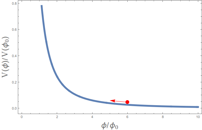
Figure 1: The potential for $s=2\epsilon$, showing field evolution.

In the next section, we demonstrate that this solution is a dynamical attractor, and discuss cosmological boundary conditions.

4 General Field Dynamics

4.1 Attractor Behavior

While it is straightforward to demonstrate that Eqs. (3.13,3.16,3.17) represent a solution for field evolution in a Lagrangian of the form (3.3), it is not immediately clear that this solution represents a dynamical attractor, which is necessary for the construction of a viable Dark Energy model. In this section, we demonstrate that the solution is, in fact, a dynamical attractor.

The equation of motion for a Lagrangian of the form (3.3) can be shown to be:

$$\ddot{\phi}+3\frac{H}{\gamma^{2}}\dot{\phi}+\frac{3}{2}\frac{f^{\prime}\left(\phi\right)}{f\left(\phi\right)}\dot{\phi}^{2}+\frac{f^{\prime}\left(\phi\right)}{f\left(\phi\right)^{2}}-\frac{1}{\gamma^{3}}\left[\frac{f^{\prime}\left(\phi\right)}{f\left(\phi\right)^{2}}+V^{\prime}\left(\phi\right)\right]=0,$$ (4.1)

where

$$\gamma\equiv c_{s}^{-1}=\frac{1}{\sqrt{1+f\left(\phi\right)\dot{\phi}^{2}}}.$$ (4.2)

We can write this in dimensionless phase-space variables as follows: Take

$$x\equiv\frac{\phi}{\phi_{0}},$$ (4.3)

and

$$y=y(x)=\frac{\dot{\phi}}{\sqrt{3}M_{\rm P}H_{0}},$$ (4.4)

where we take $x(t)$ to be monotonic, so $y(t)=y[x(t)]=y(x)$. We can likewise define dimensionless forms for the warp factor (3.16) and potential (3.17) as

$$g\left(x\right)\equiv 3M_{\rm P}^{2}H_{0}^{2}f\left(\phi\right)=\frac{3}{2\epsilon}x^{4\epsilon/s-2}\left(1-x^{4}\right),$$ (4.5)

and

$$v(x)\equiv\frac{V\left(\phi\right)}{3M_{\rm P}^{2}H_{0}^{2}}=x^{-4\epsilon/s}\left(1-\frac{2\epsilon}{3}\frac{1}{1+x^{2}}\right).$$ (4.6)

Using (4.4), we can write

$$\ddot{\phi}=\dot{\phi}\frac{d\dot{\phi}}{d\phi}=\frac{3M_{\rm P}^{2}H_{0}^{2}}{\phi_{0}}y(x)y^{\prime}(x),$$ (4.7)

and defining

$$h(x)\equiv H/H_{0},$$ (4.8)

we can write a general dimensionless equation for evolution of the system in phase space, appropriate for numerical evolution:

$$y(x)y^{\prime}(x)+3\sqrt{-\frac{8\epsilon}{3s^{2}}}\frac{h(x)y(x)}{\gamma^{2}\left(x\right)}+\frac{g^{\prime}\left(x\right)}{g\left(x\right)}\left[\frac{3}{2}g\left(x\right)y^{2}\left(x\right)+\left(1-\frac{1}{\gamma^{3}\left(x\right)}\right)\right]-\frac{v^{\prime}\left(x\right)}{\gamma^{3}\left(x\right)}=0.$$ (4.9)

The analytic solution (3.13) then corresponds to

$$c_{S}\left(x\right) =\gamma^{-1}\left(x\right)=x^{2},$$ (4.10)

$$h\left(x\right) =x^{-2\epsilon/s},$$ (4.11)

$$y\left(x\right) =\pm\sqrt{-\frac{2\epsilon}{3}}x^{1-2\epsilon/s},$$ (4.12)

where the sign of $y\left(x\right)$ is the same as the sign of $s$. It is straightforward to verify that this is an exact solution to Eq. (4.9).

We are particularly interested in the case $s=2\epsilon$, (3.19,3.21,3.24), which corresponds to

$$g\left(x\right)=\frac{3}{2\epsilon}\left(1-x^{4}\right),$$ (4.13)

$$v(x)=x^{-2}\left(1-\frac{2\epsilon}{3}\frac{1}{1+x^{2}}\right),$$ (4.14)

with analytic solution

$$c_{S}\left(x\right) =\gamma^{-1}\left(x\right)=x^{2},$$ (4.15)

$$h\left(x\right) =x^{-1},$$ (4.16)

$$y\left(x\right) =-\sqrt{-\frac{2\epsilon}{3}}={\rm const.}$$ (4.17)

We evaluate the full equation of motion (4.9) for a fiducial case of $\epsilon=-0.435$, corresponding to the best-fit value of $w=-1.29$ from the analysis of Di Valentino, et al. [5]. Figure 2 shows $y(x)$ vs $x$ for a variety of initial conditions, showing the attractor behavior of the solution (4.15). Figure 3 shows the same attractor solution as a function of scale factor $a$ instead of as a function of the field, showing rapid convergence to the attractor solution.

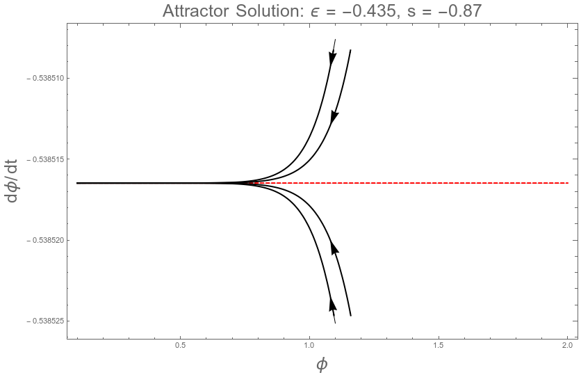
Figure 2: Phase space plot of attractor behavior for the phantom scalar field. The dotted (red) line represents the late-time attractor solution, and the solid lines represent exact numerical solutions for the field evolution. Note that the field is rolling up the potential, with $\dot{\phi}<0$.

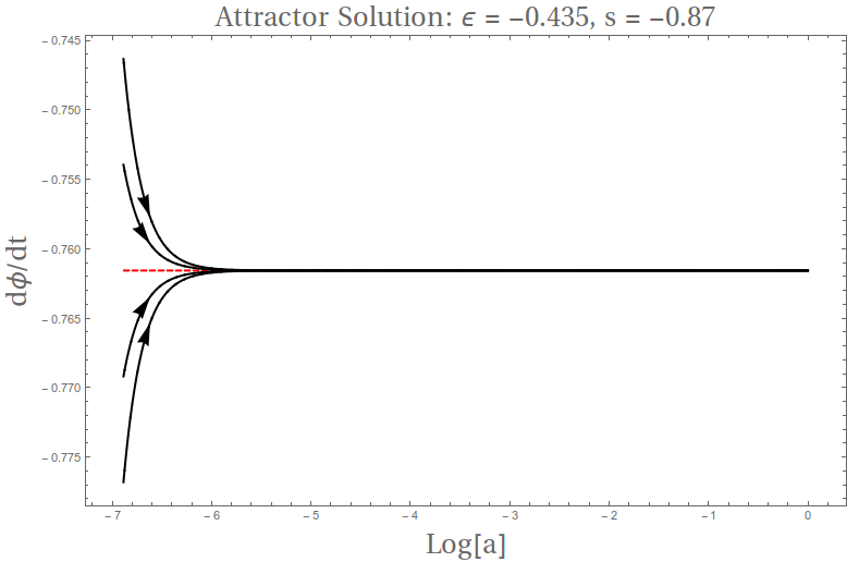
Figure 3: Attractor behavior for the phantom scalar field, plotted vs. scale factor $a$. The dotted (red) line represents the late-time attractor solution, and the solid lines represent exact numerical solutions for the field evolution.

4.2 Cosmological Boundary Conditions

With attractor behavior established, we now consider the question of cosmological boundary condition. Our exact solution (3.13,3.16,3.17) only applies to a single-component universe, i.e. it is a good approximation in the limit that Dark Energy dominates the cosmological energy density, and therefore the dynamics. However, in the presence of Dark Matter, the Dark Energy will be subdominant at high redshift, with the transition from matter- to phantom-domination happening at an approximate redshift of $z\sim 1$. We must therefore consider the dynamics of the field in the limit of matter-domination, which sets the boundary condition for the field evolution when the phantom energy dominates, at $z<1$.

Consider the limit of large field, $x\gg 1$, so that the dimensionless warp factor (4.5) and potential (4.6) become

$$g(x)\frac{3}{2\epsilon}\left(1-x^{4}\right)\rightarrow-\frac{3}{2\epsilon}x^{4},$$ (4.18)

$$v(x)=x^{-2}\left(1-\frac{2\epsilon}{3}\frac{1}{1+x^{2}}\right)\rightarrow x^{-2}.$$ (4.19)

We consider by ansatz a solution of the form $y\left(x\right)\rightarrow 0$. It is straightforward to identify subdominant terms in the equation of motion (4.9),

$$\frac{g^{\prime}}{g}\rightarrow\frac{4}{x}\rightarrow 0,$$ (4.20)

$$\frac{g^{\prime}}{g^{2}}\rightarrow 0,$$ (4.21)

$$y\left(x\right)y^{\prime}\left(x\right)\rightarrow 0,$$ (4.22)

$$c_{S}^{2}=\gamma^{-2}=1+g\left(x\right)y\left(x\right)\rightarrow 1.$$ (4.23)

In this limit, the solution is a slowly rolling scalar,

$$3H(t){\dot{x}}-v^{\prime}\left(x\right)=0,$$ (4.24)

where $H\left(t\right)$ is determined by the scaling of the dominant energy component, either matter or radiation. Taking

$$H\left(t\right)=\frac{2}{3\left(1+w\right)}t^{-1},$$ (4.25)

and $v\left(x\right)=x^{-2}$, the solution to (4.24) is

$$x\left(t\right)\propto\left(1-Ct^{2}\right)^{1/4}\rightarrow\mathrm{const.}$$ (4.26)

This solution is confirmed by direct numerical integration of the full equation of motion (4.9). We therefore have a boundary condition of a frozen field with $c_{S}=1$ in the very early universe, which then relaxes to the attractor solution once the phantom component becomes dominant. Figure 4 shows field relaxation to the attractor solution with a cosmological boundary condition, $\dot{\phi}\rightarrow 0$, showing that relaxation occurs rapidly, in less than a Hubble time.

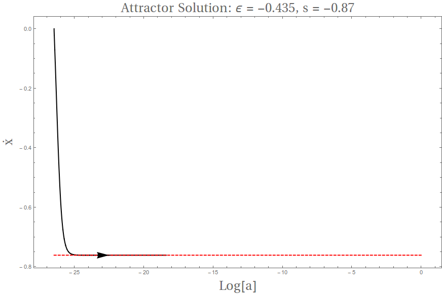
Figure 4: Field evolution with a cosmological boundary condition $\dot{\phi}\rightarrow 0$. (Scale factor is in arbitrary units.) The dotted (red) line represents the late-time attractor solution.

4.3 Vacuum Stability in Arbitrary Gauge

We have shown that, considered in the fluid rest frame, the energy density (2.3) (and therefore the field Hamiltonian) is bounded from below, with a stable dynamical attractor solution corresponding to $p=w\rho$, which $w={\mathrm{c}onst.}<-1$. The expression

$$\rho=2X{\mathcal{L}}_{X}-{\mathcal{L}}$$ (4.27)

is manifestly a coordinate scalar, and independent of gauge. However, the Hamiltonian is a coordinate-dependent object, corresponding to the time-evolution operator in a particlar foliation of the spacetime. For a perfect fluid, the Hamiltonian corresponds exactly to the energy density (3.5) in the rest frame of the fluid, where $T^{\mu}{}_{\nu}={\mathrm{d}iag}\left(\rho,-p,-p,-p\right)$, and

$${\mathcal{H}}\equiv T^{0}{}_{0}=\rho.$$ (4.28)

The fluid four-velocity in a general coordinate frame can be written as

$$u^{\mu}=\frac{\partial^{\mu}\phi}{\sqrt{2X}},$$ (4.29)

which is by construction timelike and unit normalized, $u^{\mu}u_{\mu}=+1$. (Note that timelike $u^{\mu}$ automatically implies that the kinetic term $X$ is positive-definite). The corresponding stress-energy is then

$$T^{\mu\nu} = \left(\rho+p\right)u^{\mu}u^{\nu}-g^{\mu\nu}p$$ (4.30)

$$= {\mathcal{L}}_{X}\partial^{\mu}\phi\partial^{\nu}\phi-g^{\mu\nu}{\mathcal{L}}$$ (4.31)

$$= -\frac{\partial^{\mu}\phi\partial^{\nu}\phi}{\sqrt{1+2f\left(\phi\right)X}}-g^{\mu\nu}{\mathcal{L}}.$$ (4.32)

We can then write the Hamiltonian in a general coordinate frame as

$${\mathcal{H}} = V\left(\phi\right)-\frac{1}{f\left(\phi\right)}+\frac{1+f\left(\phi\right)\left(\partial^{i}\phi\right)\left(\partial_{i}\phi\right)}{f\left(\phi\right)\sqrt{1+2f\left(\phi\right)X}}$$ (4.33)

$$= \rho-\frac{\left(\nabla\phi\right)^{2}}{c_{S}}.$$ (4.34)

where $\left(\partial^{i}\phi\right)\left(\partial_{i}\phi\right)=-\left(\nabla\phi\right)^{2}$ denotes a sum over spatial indices. This reduces trivially to Eq. (3.5) in the limit of zero field gradient $\partial^{i}\phi=0$, i.e. the rest frame of the fluid. This is in general not positive definite, since a negative Hamiltonian density can be found for a field configuration with gradient

$$(\nabla\phi)^{2}>\rho c_{s}=\frac{1}{f\left(\phi\right)}\left(1-c_{S}\right)+c_{S}V\left(\phi\right).$$ (4.35)

For the solution (4.15), this condition is especially simple, since

$$\frac{\rho}{3M_{\rm P}^{2}}=h^{2}\left(x\right)=\gamma\left(x\right)=\frac{1}{c_{S}},$$ (4.36)

so that

$$c_{S}\rho=3M_{P}^{2}H_{0}^{2}=\mathrm{const.},$$ (4.37)

and ${\mathcal{H}}<0$ for

$$(\nabla\phi)^{2}>3M_{P}^{2}H_{0}^{2}.$$ (4.38)

While this relation shows that the Hamiltonian can be negative for sufficiently large field gradient, it does not show that the Hamiltonian is in fact unbounded. We show this below for a general NEC-violating perfect fluid, and apply the result to the specific model considered here.

The general case was shown by Sawiki and Vikman in Ref. [82]. Consider a perfect fluid with stress-energy violating the Null Energy Condition, such that there exists a null congruence $n^{\mu}$ such that

$$T_{\mu\nu}n^{\mu}n^{\nu}<0.$$ (4.39)

Take the fluid four-velocity to by given by a timelike congruence $u^{\mu}$. The rest-frame energy density $\rho$ is then given by

$$\rho=T_{\mu\nu}u^{\mu}u^{\nu}=2X{\mathcal{L}}_{X}-{\mathcal{L}}.$$ (4.40)

This is a coordinate-invariant scalar, and is valid in any reference frame. However, it is only equal to the Hamiltonian in the rest frame of the fluid, $u^{\mu}=(1,0,0,0)$. Now consider an arbitrary coordinate frame defined by a timelike congruence $v^{\mu}:\ v^{\mu}v_{\mu}=+1$. The Hamiltonian defined by this rest frame is given by

$${\mathcal{H}}=T_{\mu\nu}v^{\mu}v^{\nu}.$$ (4.41)

We now construct $v^{\mu}$ as a linear combination of the fluid four-velocity $u^{\mu}$ and null vector $n^{\mu}$,

$$v^{\mu}\equiv\alpha u^{\mu}+\beta n^{\mu},$$ (4.42)

where $\alpha$ and $\beta$ are constants, and $n^{\mu}$ is normalized such that $u^{\mu}n_{\mu}=+1$. Since $v_{\mu}$ is by definition unit normalized,

$$v^{\mu}v_{\mu}=+1 =\alpha^{2}u^{\mu}u_{\mu}+2\alpha\beta u^{\mu}n_{\mu}+\beta^{2}n^{\mu}n_{\mu}$$ (4.44)

$$=\alpha^{2}+2\alpha\beta,$$

so that

$$\beta=\frac{1-\alpha^{2}}{2\alpha},$$ (4.45)

and

$$v^{\mu}=\alpha u^{\mu}+\frac{1-\alpha^{2}}{2\alpha}n^{\mu}.$$ (4.46)

The corresponding Hamiltonian is then

$${\mathcal{H}}=\alpha^{2}T_{\mu\nu}u^{\mu}u^{\nu}+(1-\alpha^{2})T_{\mu\nu}u^{\mu}n^{\nu}+\frac{(1-\alpha^{2})^{2}}{4\alpha^{2}}T_{\mu\nu}n^{\mu}n^{\nu}.$$ (4.47)

Note that if $n^{\mu}$ satisfies the NEC, the last term is zero or positive-definite, but if $n^{\mu}$ violates the NEC, it is negative,

$$T_{\mu\nu}n^{\mu}n^{\nu}<0.$$ (4.48)

We are free to take the limit that $v^{\mu}$ is arbitrarily close to the light cone, $v^{\mu}\rightarrow n^{\mu}$, which corresponds to the limit $\alpha\rightarrow 0$. Then the Hamiltonian approaches

$${\mathcal{H}}\rightarrow\frac{1}{4\alpha^{2}}T_{\mu\nu}n^{\mu}n^{\nu}\rightarrow-\infty.$$ (4.49)

The vector $v^{\mu}$ remains timelike and unit normalized, but the Hamiltonian is unbounded from below. For the particular case of the scalar field Lagrangian (3.3),

(4.50)

(4.51)

(4.52)

Then Eq. (4.47) reduces to

$${\mathcal{H}}=\rho+\frac{(1-\alpha^{2})^{2}}{2\alpha^{2}}X\mathcal{L}_{X}\rightarrow-\frac{1}{2\alpha^{2}}\frac{X}{c_{S}},\ \alpha\rightarrow 0.$$ (4.53)

Therefore, while the field Hamiltonian is bounded and well-behaved in the rest frame of the fluid, there exists a proper Lorentz frame for which the Hamiltonian appears unbounded from below.

5 Conclusions

Current data suggest a tension between high-redshift constraints on the Hubble parameter $H_{0}$ from Cosmic Microwave Backround measurements [1], and low-redshift constraints from Type-Ia supernovae [2]. While still not compelling when viewed in terms of Bayesian evidence, this discrepancy suggests the need for inclusion of extended cosmological parameters beyond $\Lambda$CDM. Perhaps the conceptually simplest way to reconcile a low value of $H_{0}$ at high redshift with a high value at low redshift is Dark Energy which violates the Null Energy Condition, such that the expansion rate $H$ increases with expansion. Such “Phantom” Dark Energy (PDE) is characterized by Equation of State $p<-\rho$; while appealing from a parametric standpoint, PDE presents serious problems from a model-building standpoint. In particular, a phantom equation of state in a scalar field theory typically requires a wrong-sign kinetic term, which implies negative energy and a vacuum unstable to particle production [79, 80, 81].

In this paper, we construct a Lagrangian with phantom equation of state $p<-\rho$, based on a Dirac-Born-Infeld (DBI) Lagrangian, with a wrong-sign kinetic term

$${\mathcal{L}}=-\frac{1}{f\left(\phi\right)}\sqrt{1+2f\left(\phi\right)X}+\frac{1}{f\left(\phi\right)}-V\left(\phi\right).$$ (5.1)

For appropriate choices of $f\left(\phi\right)$ and $V\left(\phi\right)$, the comoving energy density $\rho$ is bounded from below,

$$\rho=\frac{1}{f\left(\phi\right)\sqrt{1+2f\left(\phi\right)X}}-\frac{1}{f\left(\phi\right)}+V\left(\phi\right).$$ (5.2)

We show by construction that it is possible to construct a Lagrangian with exact solution for homogeneous field modes such that $w\equiv p/\rho={\mathrm{c}onst.}<-1$. These solutions correspond to a scalar field rolling up an approximately quadratic potential (Fig. 1). We show that these solutions correspond to a dynamical attractor in a cosmological background, and consider early-universe boundary conditions for the phantom field. We find field dynamics such that, in a matter-dominated phase at high redshift, the field is “frozen”, and only becomes dynamical when the universe transitions to Dark Energy domination at low redshift. At that point, the field dynamics transitions to the attractor dynamics in less than a Hubble time, approaching constant equation of state $w<-1$.

Since the DBI-type Lagrangian does not contain higher time-derivatives of the scalar field, the theory automatically avoids any Ostrogradsky instabilities due non-local interactions [88]. Despite these attractive features, the model is nonetheless pathological: While the field Hamiltonian is well-behaved in the rest frame of the fluid, it is dependent on the spacetime foliation. In particular, there in general exist proper Lorentz frames for which the Hamiltonian is unbounded from below [82]. This is distinct from the Unruh effect [90] in that it occurs for inertial, rather than accelerated observers. This is not necessarily an issue with repect to classical cosmological evolution, since there is no instability in the cosmological rest frame, and the classical gradient instability is nonlinear. However, quantum-mechanically, highly boosted momentum states will inevitably sample the region of phase space for which the field Hamiltonian can become arbitrarily negative [91]. Thus, while such models are attractive phenomenological descriptions of Phantom Dark Energy, they remain inconsistent as realizations of a fully fundamental theory. We note that the model considered here is purely phenomenological: wrong-sign Lagrangians are not, for example, typical of string-theory constructions [92]. It is an interesting question whether or not Lagrangians of the type considered here can be embedded in a self-consistent UV-complete theory.

References

- [1] Planck collaboration, P. A. R. Ade et al., Planck 2015 results. XIII. Cosmological parameters, Astron. Astrophys. 594 (2016) A13, [1502.01589].
- [2] A. G. Riess et al., A 2.4% Determination of the Local Value of the Hubble Constant, Astrophys. J. 826 (2016) 56, [1604.01424].
- [3] V. Bonvin et al., H0LiCOW – V. New COSMOGRAIL time delays of HE 0435−1223: to 3.8 per cent precision from strong lensing in a flat ΛCDM model, Mon. Not. Roy. Astron. Soc. 465 (2017) 4914–4930, [1607.01790].
- [4] J. L. Bernal, L. Verde and A. G. Riess, The trouble with , JCAP 1610 (2016) 019, [1607.05617].
- [5] E. Di Valentino, A. Melchiorri and J. Silk, Reconciling Planck with the local value of in extended parameter space, Phys. Lett. B761 (2016) 242–246, [1606.00634].
- [6] V. V. Luković, R. D’Agostino and N. Vittorio, Is there a concordance value for ?, Astron. Astrophys. 595 (2016) A109, [1607.05677].
- [7] M. Archidiacono, S. Gariazzo, C. Giunti, S. Hannestad, R. Hansen, M. Laveder et al., Pseudoscalar—sterile neutrino interactions: reconciling the cosmos with neutrino oscillations, JCAP 1608 (2016) 067, [1606.07673].
- [8] T. Tram, R. Vallance and V. Vennin, Inflation Model Selection meets Dark Radiation, JCAP 1701 (2017) 046, [1606.09199].
- [9] Planck collaboration, N. Aghanim et al., Planck intermediate results. LI. Features in the cosmic microwave background temperature power spectrum and shifts in cosmological parameters, Astron. Astrophys. 607 (2017) A95, [1608.02487].
- [10] P. Ko and Y. Tang, Light dark photon and fermionic dark radiation for the Hubble constant and the structure formation, Phys. Lett. B762 (2016) 462–466, [1608.01083].
- [11] M.-M. Zhao, Y.-H. Li, J.-F. Zhang and X. Zhang, Constraining neutrino mass and extra relativistic degrees of freedom in dynamical dark energy models using Planck 2015 data in combination with low-redshift cosmological probes: basic extensions to ΛCDM cosmology, Mon. Not. Roy. Astron. Soc. 469 (2017) 1713–1724, [1608.01219].
- [12] W. Cardona, M. Kunz and V. Pettorino, Determining with Bayesian hyper-parameters, JCAP 1703 (2017) 056, [1611.06088].
- [13] W. Lin and M. Ishak, Cosmological discordances: A new measure, marginalization effects, and application to geometry versus growth current data sets, Phys. Rev. D96 (2017) 023532, [1705.05303].
- [14] W. L. Freedman, Cosmology at at Crossroads: Tension with the Hubble Constant, Nat. Astron. 1 (2017) 0169, [1706.02739].
- [15] DES collaboration, T. M. C. Abbott et al., Dark Energy Survey Year 1 Results: Cosmological Constraints from Galaxy Clustering and Weak Lensing, 1708.01530.
- [16] S. Joudaki et al., KiDS-450 + 2dFLenS: Cosmological parameter constraints from weak gravitational lensing tomography and overlapping redshift-space galaxy clustering, Mon. Not. Roy. Astron. Soc. 474 (2018) 4894, [1707.06627].
- [17] B. R. Zhang, M. J. Childress, T. M. Davis, N. V. Karpenka, C. Lidman, B. P. Schmidt et al., A blinded determination of from low-redshift Type Ia supernovae, calibrated by Cepheid variables, Mon. Not. Roy. Astron. Soc. 471 (2017) 2254–2285, [1706.07573].
- [18] S. M. Feeney, D. J. Mortlock and N. Dalmasso, Clarifying the Hubble constant tension with a Bayesian hierarchical model of the local distance ladder, 1707.00007.
- [19] G. E. Addison, D. J. Watts, C. L. Bennett, M. Halpern, G. Hinshaw and J. L. Weiland, Elucidating CDM: Impact of Baryon Acoustic Oscillation Measurements on the Hubble Constant Discrepancy, Astrophys. J. 853 (2018) 119, [1707.06547].
- [20] A. E. Romano, Hubble trouble or Hubble bubble?, 1609.04081.
- [21] A. Shafieloo and D. K. Hazra, Consistency of the Planck CMB data and CDM cosmology, JCAP 1704 (2017) 012, [1610.07402].
- [22] J. Calcino and T. Davis, The need for accurate redshifts in supernova cosmology, JCAP 1701 (2017) 038, [1610.07695].
- [23] M. Lattanzi, C. Burigana, M. Gerbino, A. Gruppuso, N. Mandolesi, P. Natoli et al., On the impact of large angle CMB polarization data on cosmological parameters, JCAP 1702 (2017) 041, [1611.01123].
- [24] P. Fleury, C. Clarkson and R. Maartens, How does the cosmic large-scale structure bias the Hubble diagram?, JCAP 1703 (2017) 062, [1612.03726].
- [25] I. Odderskov, S. Hannestad and J. Brandbyge, The variance of the locally measured Hubble parameter explained with different estimators, JCAP 1703 (2017) 022, [1701.05391].
- [26] A. Heavens, Y. Fantaye, E. Sellentin, H. Eggers, Z. Hosenie, S. Kroon et al., No evidence for extensions to the standard cosmological model, Phys. Rev. Lett. 119 (2017) 101301, [1704.03467].
- [27] H.-Y. Wu and D. Huterer, Sample variance in the local measurements of the Hubble constant, Mon. Not. Roy. Astron. Soc. 471 (2017) 4946–4955, [1706.09723].
- [28] J. F. Jesus, T. M. Gregório, F. Andrade-Oliveira, R. Valentim and C. A. O. Matos, Bayesian correction of data uncertainties, 1709.00646.
- [29] W. Lin and M. Ishak, Cosmological discordances II: Hubble constant, Planck and large-scale-structure data sets, Phys. Rev. D96 (2017) 083532, [1708.09813].
- [30] Z. Hou et al., A Comparison of Maps and Power Spectra Determined from South Pole Telescope and Planck Data, Astrophys. J. 853 (2018) 3, [1704.00884].
- [31] SPT collaboration, K. Aylor et al., A Comparison of Cosmological Parameters Determined from CMB Temperature Power Spectra from the South Pole Telescope and the Planck Satellite, Astrophys. J. 850 (2017) 101, [1706.10286].
- [32] B. Follin and L. Knox, Insensitivity of The Distance Ladder Hubble Constant Determination to Cepheid Calibration Modeling Choices, 1707.01175.
- [33] N. Sasankan, M. R. Gangopadhyay, G. J. Mathews and M. Kusakabe, New observational limits on dark radiation in braneworld cosmology, Phys. Rev. D95 (2017) 083516, [1607.06858].
- [34] L. Feng, J.-F. Zhang and X. Zhang, Searching for sterile neutrinos in dynamical dark energy cosmologies, 1706.06913.
- [35] E. Di Valentino and F. R. Bouchet, A comment on power-law inflation with a dark radiation component, JCAP 1610 (2016) 011, [1609.00328].
- [36] G. Barenboim, W. H. Kinney and W.-I. Park, Flavor versus mass eigenstates in neutrino asymmetries: implications for cosmology, Eur. Phys. J. C77 (2017) 590, [1609.03200].
- [37] M. Gerbino, K. Freese, S. Vagnozzi, M. Lattanzi, O. Mena, E. Giusarma et al., Impact of neutrino properties on the estimation of inflationary parameters from current and future observations, Phys. Rev. D95 (2017) 043512, [1610.08830].
- [38] L. Verde, E. Bellini, C. Pigozzo, A. F. Heavens and R. Jimenez, Early Cosmology Constrained, JCAP 1704 (2017) 023, [1611.00376].
- [39] M. Benetti, L. L. Graef and J. S. Alcaniz, Do joint CMB and HST data support a scale invariant spectrum?, JCAP 1704 (2017) 003, [1702.06509].
- [40] L. Feng, J.-F. Zhang and X. Zhang, A search for sterile neutrinos with the latest cosmological observations, Eur. Phys. J. C77 (2017) 418, [1703.04884].
- [41] M.-M. Zhao, D.-Z. He, J.-F. Zhang and X. Zhang, Search for sterile neutrinos in holographic dark energy cosmology: Reconciling Planck observation with the local measurement of the Hubble constant, Phys. Rev. D96 (2017) 043520, [1703.08456].
- [42] C. Brust, Y. Cui and K. Sigurdson, Cosmological Constraints on Interacting Light Particles, JCAP 1708 (2017) 020, [1703.10732].
- [43] S. Gariazzo, M. Escudero, R. Diamanti and O. Mena, Cosmological searches for a noncold dark matter component, Phys. Rev. D96 (2017) 043501, [1704.02991].
- [44] N. Sasankan, M. R. Gangopadhyay, G. J. Mathews and M. Kusakabe, Limits on Brane-World and Particle Dark Radiation from Big Bang Nucleosynthesis and the CMB, Int. J. Mod. Phys. E26 (2017) 1741007, [1706.03630].
- [45] O. Farooq, F. R. Madiyar, S. Crandall and B. Ratra, Hubble Parameter Measurement Constraints on the Redshift of the Deceleration–acceleration Transition, Dynamical Dark Energy, and Space Curvature, Astrophys. J. 835 (2017) 26, [1607.03537].
- [46] Y.-Y. Xu and X. Zhang, Comparison of dark energy models after Planck 2015, Eur. Phys. J. C76 (2016) 588, [1607.06262].
- [47] D.-M. Xia and S. Wang, Constraining interacting dark energy models with latest cosmological observations, Mon. Not. Roy. Astron. Soc. 463 (2016) 952–956, [1608.04545].
- [48] S. Kumar and R. C. Nunes, Probing the interaction between dark matter and dark energy in the presence of massive neutrinos, Phys. Rev. D94 (2016) 123511, [1608.02454].
- [49] T. Karwal and M. Kamionkowski, Dark energy at early times, the Hubble parameter, and the string axiverse, Phys. Rev. D94 (2016) 103523, [1608.01309].
- [50] Z. Chacko, Y. Cui, S. Hong, T. Okui and Y. Tsai, Partially Acoustic Dark Matter, Interacting Dark Radiation, and Large Scale Structure, JHEP 12 (2016) 108, [1609.03569].
- [51] R. J. F. Marcondes, Interacting dark energy models in Cosmology and large-scale structure observational tests. PhD thesis, 2016. 1610.01272.
- [52] C. van de Bruck, J. Mifsud and J. Morrice, Testing coupled dark energy models with their cosmological background evolution, Phys. Rev. D95 (2017) 043513, [1609.09855].
- [53] R. Murgia, Constraining the interaction between dark matter and dark energy with CMB data, in Proceedings, 7th Young Researchers Meeting (YRM 2016): Torino, Italy, October 24-26, 2016, 2016. 1612.02282.
- [54] J. Sola, A. Gomez-Valent and J. de Cruz Pérez, Dynamical dark energy: scalar fields and running vacuum, Mod. Phys. Lett. A32 (2017) 1750054, [1610.08965].
- [55] G.-B. Zhao et al., Dynamical dark energy in light of the latest observations, Nat. Astron. 1 (2017) 627–632, [1701.08165].
- [56] S. Kumar and R. C. Nunes, Echo of interactions in the dark sector, Phys. Rev. D96 (2017) 103511, [1702.02143].
- [57] J. Sola, J. d. C. Perez and A. Gomez-Valent, Towards the firsts compelling signs of vacuum dynamics in modern cosmological observations, 1703.08218.
- [58] Y. Zhang, H. Zhang, D. Wang, Y. Qi, Y. Wang and G.-B. Zhao, Probing dynamics of dark energy with latest observations, Res. Astron. Astrophys. 17 (2017) 050, [1703.08293].
- [59] E. Di Valentino, A. Melchiorri, E. V. Linder and J. Silk, Constraining Dark Energy Dynamics in Extended Parameter Space, Phys. Rev. D96 (2017) 023523, [1704.00762].
- [60] S. Camera, M. Martinelli and D. Bertacca, Easing Tensions with Quartessence, 1704.06277.
- [61] E. Di Valentino, A. Melchiorri and O. Mena, Can interacting dark energy solve the tension?, Phys. Rev. D96 (2017) 043503, [1704.08342].
- [62] M. Carrillo González and M. Trodden, Field Theories and Fluids for an Interacting Dark Sector, Phys. Rev. D97 (2018) 043508, [1705.04737].
- [63] S. Dhawan, A. Goobar, E. Mörtsell, R. Amanullah and U. Feindt, Narrowing down the possible explanations of cosmic acceleration with geometric probes, JCAP 1707 (2017) 040, [1705.05768].
- [64] J. Solà, A. Gómez-Valent and J. de Cruz Pérez, The tension in light of vacuum dynamics in the Universe, Phys. Lett. B774 (2017) 317–324, [1705.06723].
- [65] W. Yang, N. Banerjee and S. Pan, Constraining a dark matter and dark energy interaction scenario with a dynamical equation of state, Phys. Rev. D95 (2017) 123527, [1705.09278].
- [66] J. Magana, M. H. Amante, M. A. Garcia-Aspeitia and V. Motta, The Cardassian expansion revisited: constraints from updated Hubble parameter measurements and Type Ia Supernovae data, 1706.09848.
- [67] A. I. Lonappan, S. Kumar, Ruchika, B. R. Dinda and A. A. Sen, Bayesian evidences for dark energy models in light of current observational data, Phys. Rev. D97 (2018) 043524, [1707.00603].
- [68] M. H. P. M. van Putten, Accelerated cosmological expansion without tension in the Hubble parameter, 2017. 1707.02588.
- [69] V. Miranda, M. Carrillo González, E. Krause and M. Trodden, Finding structure in the dark: coupled dark energy, weak lensing, and the mildly nonlinear regime, 1707.05694.
- [70] K. Bolejko, Emergence of spatial curvature, 1707.01800.
- [71] J. Ooba, B. Ratra and N. Sugiyama, Planck 2015 constraints on the non-flat CDM inflation model, 1707.03452.
- [72] K. Bolejko, Relativistic numerical cosmology with Silent Universes, Class. Quant. Grav. 35 (2018) 024003, [1708.09143].
- [73] R. R. Caldwell, A Phantom menace?, Phys. Lett. B545 (2002) 23–29, [astro-ph/9908168].
- [74] R. R. Caldwell, M. Kamionkowski and N. N. Weinberg, Phantom energy and cosmic doomsday, Phys. Rev. Lett. 91 (2003) 071301, [astro-ph/0302506].
- [75] M. P. Dabrowski and T. Stachowiak, Phantom Friedmann cosmologies and higher-order characteristics of expansion, Annals Phys. 321 (2006) 771–812, [hep-th/0411199].
- [76] U. Alam, S. Bag and V. Sahni, Constraining the Cosmology of the Phantom Brane using Distance Measures, Phys. Rev. D95 (2017) 023524, [1605.04707].
- [77] J. Ooba, B. Ratra and N. Sugiyama, Planck 2015 constraints on spatially-flat dynamical dark energy models, 1802.05571.
- [78] V. Faraoni, Phantom cosmology with general potentials, Class. Quant. Grav. 22 (2005) 3235–3246, [gr-qc/0506095].
- [79] S. M. Carroll, M. Hoffman and M. Trodden, Can the dark energy equation - of - state parameter w be less than -1?, Phys. Rev. D68 (2003) 023509, [astro-ph/0301273].
- [80] J. M. Cline, S. Jeon and G. D. Moore, The Phantom menaced: Constraints on low-energy effective ghosts, Phys. Rev. D70 (2004) 043543, [hep-ph/0311312].
- [81] S. Dubovsky, T. Gregoire, A. Nicolis and R. Rattazzi, Null energy condition and superluminal propagation, JHEP 03 (2006) 025, [hep-th/0512260].
- [82] I. Sawicki and A. Vikman, Hidden Negative Energies in Strongly Accelerated Universes, Phys. Rev. D87 (2013) 067301, [1209.2961].
- [83] R. Bean, D. J. H. Chung and G. Geshnizjani, Reconstructing a general inflationary action, Phys. Rev. D78 (2008) 023517, [0801.0742].
- [84] D. Bessada, W. H. Kinney, D. Stojkovic and J. Wang, Tachyacoustic Cosmology: An Alternative to Inflation, Phys. Rev. D81 (2010) 043510, [0908.3898].
- [85] W. H. Kinney and K. Tzirakis, Quantum modes in DBI inflation: exact solutions and constraints from vacuum selection, Phys. Rev. D77 (2008) 103517, [0712.2043].
- [86] C. Csaki, N. Kaloper and J. Terning, The Accelerated acceleration of the Universe, JCAP 0606 (2006) 022, [astro-ph/0507148].
- [87] M. Sahlen, A. R. Liddle and D. Parkinson, Direct reconstruction of the quintessence potential, Phys. Rev. D72 (2005) 083511, [astro-ph/0506696].
- [88] M. Ostrogradsky, Mémoires sur les équations différentielles, relatives au problème des isopérimètres, Mem. Acad. St. Petersbourg 6 (1850) 385–517.
- [89] R. P. Woodard, Ostrogradsky’s theorem on Hamiltonian instability, Scholarpedia 10 (2015) 32243, [1506.02210].
- [90] W. G. Unruh, Notes on black hole evaporation, Phys. Rev. D14 (1976) 870.
- [91] D. A. Easson and A. Vikman, The Phantom of the New Oscillatory Cosmological Phase, 1607.00996.
- [92] S. Chatterjee, M. Parikh and J. P. van der Schaar, On Coupling NEC-Violating Matter to Gravity, Phys. Lett. B744 (2015) 34–37, [1503.07950].