A Locking-free DP-Q2-P1 MFEM for
Incompressible Nonlinear Elasticity Problems

Abstract

A mixed finite element method (MFEM), using dual-parametric piecewise biquadratic and affine (DP-Q2-P1) finite element approximations for the deformation and the pressure like Lagrange multiplier respectively, is developed and analyzed for the numerical computation of incompressible nonlinear elasticity problems with large deformation gradient, and a damped Newton method is applied to solve the resulted discrete problem. The method is proved to be locking free and stable. The accuracy and efficiency of the method are illustrated by numerical experiments on some typical cavitation problems.

Key words: DP-Q2-P1 mixed finite element, damped Newton method, locking-free, incompressible nonlinear elasticity, large deformation gradient

1 Introduction

For incompressible elasticity, it is well known that, even in the case of small deformation and linear elasticity, the notorious volume locking can happen and ultimately leads to the failure of some finite element approximations [11, 12, 13, 14]. In the case of incompressible linear elasticity, it is well-known how to overcome locking numerically, for example, by using the enhanced assumed strain methods to increase the degrees of freedom of the elements [16, 17], by using the nonconforming finite element methods to weakening the global continuity of the numerical solutions [1], or by using the mixed finite element methods (MFEMs) to relax the constraint of the incompressibility on the numerical solutions [11, 18], etc.. However, for incompressible nonlinear elasticity, especially for large deformation gradient problems which will be addressed in this paper, there still lack of systematic results.

Let $\Omega\subset\mathbb{R}^{2}$ be a bounded open domain with smooth boundary occupied by an isotropic hyper-elastic body in its reference configuration. Let the stored energy density function of the material $W(\nabla\bm{u}):M_{+}^{2\times 2}\to\mathrm{R}^{+}$ be poly-convex, where $\bm{u}$ is a deformation field and $M_{+}^{2\times 2}$ is the set of $2\times 2$ matrices with positive eigenvalues. Since the material is incompressible, the deformation field must satisfy the constraint $\det\nabla\bm{u}=1\ a.e.$ in $\Omega$. In the mixed formulation of nonlinear hyper-elasticity boundary value problems, one considers to solve the saddle point problem

$$(\bm{\tilde{u}},\tilde{p})=\arg\inf_{\bm{u}\in\mathcal{A}}\sup_{p\in L^{2}(\Omega)}E(\bm{u},p),$$ (1.1)

where $p$ is the pressure like Lagrangian multiplier (see [11]), $E(\bm{u},p)$ is the Lagrangian functional defined as

$$E(\bm{u},p)=\int_{\Omega}\left(W(\nabla\bm{u}(\bm{x}))-p(\det\nabla u-1)\right)\,\mathrm{d}\bm{x}-\int_{\partial_{N}\Omega}\bm{t}\cdot\bm{u}\,\mathrm{d}s,$$ (1.2)

with $\bm{t}$ the traction imposed on the Neumann boundary $\partial_{N}\Omega$, and where the set of admissible deformation functions $\mathcal{A}$ is given by

$$\mathcal{A}=\begin{cases}\{\bm{u}\in W^{1,s}(\Omega;\mathbb{R}^{2})\ \mbox{is 1-to-1 a.e.}:\bm{u}|_{\partial_{D}\Omega}=\bm{u}_{0},\},&\text{if $\partial_{D}\Omega\neq\emptyset$,}\\ \{\bm{u}\in W^{1,s}(\Omega;\mathbb{R}^{2})\ \mbox{is 1-to-1 a.e.}:\int_{\Omega}\bm{u}\,\mathrm{d}\bm{x}=\bm{0},\},&\text{otherwise,}\end{cases}$$ (1.3)

where $s>1$ is a given Sobolev index, and $\partial_{D}\Omega$ is the Dirichlet boundary with its 1-D measure $|\partial_{D}\Omega|\neq 0$.

The variational form of the Euler-Lagrange equation, i.e. the equilibrium equation, of the mixed formulation (1.1), can be expressed as

$$\left\{\begin{aligned} \int_{\Omega}\left(\dfrac{\partial W(\nabla\bm{u})}{\partial\nabla\bm{u}}:\nabla\bm{v}-p\left(\operatorname{cof}\nabla\bm{u}:\nabla\bm{v}\right)\right)\,\mathrm{d}\bm{x}&=\int_{\partial_{N}\Omega}\bm{t}\cdot\bm{v}\,\mathrm{d}s,\quad\forall\bm{v}\in\mathcal{X}_{0},\\ \int_{\Omega}q\left(\det\nabla\bm{u}-1\right)\,\mathrm{d}\bm{x}&=0,\quad\qquad\qquad\;\;\;\forall q\in\mathcal{M},\end{aligned}\right.$$ (1.4)

where $\operatorname{cof}\nabla\bm{u}$ denotes the cofactor matrix of $\nabla\bm{u}$, and

$$\mathcal{M}:=L^{2}(\Omega),\;\;\;\mathcal{X}_{0}=\begin{cases}\left\{\bm{v}\in H^{1}(\Omega;\mathbb{R}^{2}):\bm{v}|_{\partial_{D}\Omega}=\bm{0}\right\},&\text{if $\partial_{D}\Omega\neq\emptyset$},\\ \left\{\bm{v}\in H^{1}(\Omega;\mathbb{R}^{2}):\int_{\Omega}\bm{v}\,\mathrm{d}\bm{x}=\bm{0}\right\},&\text{otherwise},\\ \end{cases}$$ (1.5)

are the test function spaces for the pressure $p$ and deformation $\bm{u}$ respectively.

In the present paper, based on the variational form of Euler-Lagrange equation (1.4), a mixed finite element method (MFEM), using dual-parametric piecewise biquadratic and affine (DP-Q2-P1) finite element approximations for the deformation $\bm{u}$ and pressure like Lagrangian multiplier $p$ respectively, is developed and analyzed for the numerical computation of incompressible nonlinear elasticity boundary value problems with large deformation gradient, and a damped Newton method is applied to solve the resulted discrete problem. The method is shown to be stable (locking free) under some reasonable assumptions on the mesh regularity (see (M1) and (M2) in § 2.1), the damping criteria (see (C1) and (C2) in § 2.2) and the stability hypothesis on the mixed formulation (see (H) in § 2.3). The performance of a DP-Q2-P1 method applied to a cavitation problem, which shows an extremely large anisotropic deformation near the cavity surface, is illustrated by numerical experiments and results. We would like to point out here that the classical stability analysis for Q2-P1 element based on the divergence free argument do not directly apply to nonlinear elasticity problems with finite deformation (see for example [18]), especially those with very large nearly singular deformation gradients (see § 2.3 for details). The advantage of using the dual-parametric finite elements is that the elements can well accommodate very large anisotropic deformation as well as complex physical domain with a reasonable number of degrees of freedom [6, 7, 9].

The rest of the paper is organized as follows. § 2 is devoted to the construction of the DP-Q2-P1 MFEM and its stability analysis. In § 3, the DP-Q2-P1 mixed finite element method is applied to a cavitation problem, and the accuracy and efficiency of the method is demonstrated by the numerical results. Some concluding remarks are given in § 4.

2 The mixed finite element method and its stability

2.1 The DP-Q2-P1 mixed finite element

Let $(\hat{T},\hat{P},\hat{\Sigma})$ be the standard biquadratic-linear mixed rectangular element with

$$\begin{cases}\hat{T}=[-1,1]\times[-1,1],\\ \hat{P}=\{Q_{2}(\hat{T}),P_{1}(\hat{T})\},\\ \hat{\Sigma}=\{\bm{\hat{u}}(\hat{a}_{i}),0\leq i\leq 8;\;\;\hat{p}(\hat{b}_{0}),\partial_{\hat{x}_{1}}\hat{p}(\hat{b}_{0}),\partial_{\hat{x}_{2}}\hat{p}(\hat{b}_{0})\},\end{cases}$$

where $\{\hat{a}_{i}\}_{i=0}^{3}$ are the vertices of $\hat{T}$, $\{\hat{a}_{i}\}_{i=4}^{7}$ represent the nodes on the middle points of the corresponding edges of $\hat{T}$, and $\hat{a}_{8}=\hat{b}_{0}=(0,0)$, as shown in Figure 2.

Given 4 non-degenerate vertices $\{a_{i}\}_{i=0}^{3}$ in anticlockwise order, 5 properly distributed vertices $\{a_{i}\}_{i=4}^{8}$, and a smooth injection $F_{T}$ satisfying $a_{i}=F_{T}(\hat{a}_{i})$, $i=0,\cdots 8$, then $T=F_{T}(\hat{T})$ defines a (curve edged) quadrilateral element (see for example Figure 2). In applications, the most commonly used $F_{T}$ are bilinear, biquadratic and trigonometric (see (3.1)).

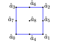
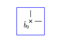
Figure 1: Reference element $\hat{T}$, $\hat{\Sigma}$.

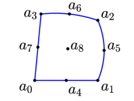
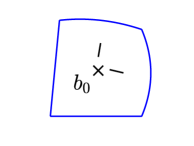
Figure 2: Element $T$, $\Sigma_{T}$.

We define the dual-parametric biquadratic-affine (DP-Q2-P1) mixed finite element $(T,P,\Sigma)$ as follows:

$$\begin{cases}T=F_{T}(\hat{T})\ \text{being a (curved) quadrilateral element,}\\ P_{T}=\big{\{}(\bm{u},p):T\to\mathbb{R}^{2}\times\mathbb{R}\ |\ \bm{u}=\hat{\bm{u}}\comp F_{T}^{-1},\hat{\bm{u}}\in Q_{2},\ p=\hat{p}\comp F_{T}^{-1},\hat{p}\in P_{1}\big{\}},\\ \Sigma_{T}=\big{\{}\bm{u}(a_{i}),a_{i}=F_{T}(\hat{a}_{i}),0\leq i\leq 8;\;p(\bm{b}_{0}),\partial_{\hat{x}_{1}}p(\hat{b}_{0})\comp F_{T}^{-1},\partial_{\hat{x}_{2}}p(\hat{b}_{0})\comp F_{T}^{-1},b_{0}=F_{T}(\hat{b}_{0})\big{\}},\end{cases}$$

and denote $\tilde{Q}_{2}\times\tilde{P}_{1}=(Q_{2}\comp F_{T}^{-1})\times(P_{1}\comp F_{T}^{-1})$.

For simplicity, we assume in this section that $\Omega=\Omega_{h}$ is properly partitioned into such quadrilateral elements, i.e. $\Omega=\Omega_{h}=\cup_{T\in\mathscr{T}_{h}}F_{T}(\hat{T})$. In addition, we assume the triangulation $\mathscr{T}_{h}$ satisfies the following regularity conditions.

(M1)

The edge lengths are of quasi-uniform, i.e. $|\wideparen{a_{0}a_{3}}|\cong|\wideparen{a_{0}a_{1}}|\cong|\wideparen{a_{1}a_{2}}|\cong|\wideparen{a_{2}a_{3}}|$, $h_{T}\cong h$,  $\forall T\in\mathscr{T}_{h}$.

(M2)

The minimum angle condition, i.e. $|\bm{l}_{1}|\cong|\bm{l}_{2}|\cong O(h_{T})$ and $h_{T}^{-2}|\bm{l}_{1}\wedge\bm{l}_{2}|\geq c>0$, $\forall T\in\mathscr{T}_{h}$, where $\bm{l}_{1}=(\vv{a_{0}a_{1}}+\vv{a_{3}a_{2}}+8\vv{a_{7}a_{5}})$ and $\bm{l}_{2}=(\vv{a_{0}a_{3}}+\vv{a_{1}a_{2}}+8\vv{a_{4}a_{6}})$.

Here and throughout the paper, $X\cong Y$, or equivalently $Y\lesssim X\lesssim Y$, means that $c^{-1}Y\leq X\leq cY$ holds for a generic constant $c\geq 1$ independent of $T$ and $h$.

Remark 1.

It is not difficult for us to show, by the standard scaling argument, that

$$|\hat{\bm{v}}|_{\gamma,2,\hat{T}}\cong h_{T}^{\gamma-1}|\bm{v}|_{\gamma,2,T},\;\;\gamma=0,1,\quad\forall T\in\mathscr{T}_{h},\;\text{and}\;\;\forall\bm{v}\in H^{1}(T;\mathbb{R}^{2})$$ (2.1)

remains valid, if $|\partial\bm{x}/\partial\bm{\hat{x}}|=|\partial F_{T}/\partial\hat{\bm{x}}|\cong h_{T}$, and $\det(\partial\bm{x}/\partial\bm{\hat{x}})\cong h_{T}^{2}$, which hold when the triangulation $\mathscr{T}_{h}$ satisfies (M1) and (M2).

2.2 The discretized problem

Define the finite element function spaces for the admissible deformation and pressure as

$$\mathcal{X}_{h}=\mathcal{A}_{h}:= \begin{cases}\left\{\bm{v}_{h}\in C(\bar{\Omega};\mathbb{R}^{2}):\;\bm{v}_{h}|_{T}\in\tilde{Q}_{2},\ \bm{v}_{h}|_{\partial_{D}\Omega}=\bm{u}_{0}\right\},\quad\;\text{if $\partial_{D}\Omega\neq\emptyset$,}\\ \left\{\bm{v}_{h}\in C(\bar{\Omega};\mathbb{R}^{2}):\;\bm{v}_{h}|_{T}\in\tilde{Q}_{2},\ \int_{\Omega}\bm{v}_{h}\,\mathrm{d}\bm{x}=\bm{0}\right\},\quad\text{otherwise,}\\ \end{cases}$$ (2.2)

$$\mathcal{M}_{h}:= \left\{p_{h}\in L^{2}(\bar{\Omega}):\;p_{h}|_{T}\in\tilde{P}_{1}\right\},$$ (2.3)

and define the finite element test function space for the deformation as

$$\mathcal{X}_{h,0}:= \begin{cases}\left\{\bm{v}_{h}\in C(\bar{\Omega};\mathbb{R}^{2}):\;\bm{v}_{h}|_{T}\in\tilde{Q}_{2},\ \bm{v}_{h}|_{\partial_{D}\Omega}=\bm{0}\right\},\quad\;\text{if $\partial_{D}\Omega\neq\emptyset$,}\\ \left\{\bm{v}_{h}\in C(\bar{\Omega};\mathbb{R}^{2}):\;\bm{v}_{h}|_{T}\in\tilde{Q}_{2},\ \int_{\Omega}\bm{v}_{h}\,\mathrm{d}\bm{x}=\bm{0}\right\},\quad\text{otherwise.}\\ \end{cases}$$ (2.4)

In the DP-Q2-P1 mixed finite element method, the equilibrium equation (1.4) is discretized into the following form

$$\left\{\begin{aligned} \int_{\Omega}\dfrac{\partial W(\nabla\bm{u}_{h})}{\partial\nabla\bm{u}_{h}}:\nabla\bm{v}_{h}-p_{h}\operatorname{cof}\nabla\bm{u}_{h}:\nabla\bm{v}_{h}\,\mathrm{d}\bm{x}&=\int_{\partial\Omega_{N}}\bm{t}\cdot\bm{v}_{h}\,\mathrm{d}s,\quad\forall\bm{v}_{h}\in\mathcal{X}_{h,0},\\ \int_{\Omega}q_{h}(\det\nabla\bm{u}_{h}-1)\,\mathrm{d}\bm{x}&=0,\qquad\qquad\qquad\;\forall q_{h}\in\mathcal{M}_{h},\end{aligned}\right.$$ (2.5)

and, in each iteration step of the damped Newton method to solve this discrete nonlinear problem, one solves the following discrete linear problem

$$\left\{\begin{aligned} \text{Find }(\bm{w}_{h},p_{h})\in\mathcal{X}_{h,0}\times\mathcal{M}_{h},\,\text{such}&\;\text{that}\\ a(\bm{w}_{h},\bm{v}_{h};\underline{\bm{u}}_{h},\underline{p}_{h})+b(\bm{v}_{h},p_{h};\bm{\underline{u}}_{h})&=f(\bm{v}_{h};\underline{\bm{u}}_{h},\underline{p}_{h}),\quad\forall\bm{v}_{h}\in\mathcal{X}_{h,0},\\ b(\bm{w}_{h},q_{h};\bm{\underline{u}}_{h})&=g(q_{h};\bm{\underline{u}}_{h}),\qquad\;\;\;\forall q_{h}\in\mathcal{M}_{h},\end{aligned}\right.$$ (2.6)

to obtain a direction modifying $(\bm{w}_{h},p_{h})$, where $\underline{\bm{u}}_{h}:=\bm{u}^{k}_{h}\in\mathcal{A}_{h}$, $\underline{p}_{h}:=p^{k}_{h}$ denotes the approximation solution obtained in the k-th iteration, and

$$a(\bm{w}_{h},\bm{v}_{h};\underline{\bm{u}}_{h},\underline{p}_{h}):=\int_{\Omega}\left(\dfrac{\partial^{2}W(\nabla\bm{u}_{h})}{\partial(\nabla\bm{u}_{h})^{2}}\Big{|}_{\bm{u}_{h}=\underline{\bm{u}}_{h}}:\nabla\bm{w}_{h}\right):\nabla\bm{v}_{h}-\underline{p}_{h}\operatorname{cof}\nabla\bm{w}_{h}:\nabla\bm{v}_{h}\,\mathrm{d}\bm{x},$$ (2.7)

$$b(\bm{v}_{h},q_{h};\underline{\bm{u}}_{h}):=\int_{\Omega}q_{h}\operatorname{cof}\nabla\underline{\bm{u}}_{h}:\nabla\bm{v}_{h}\,\mathrm{d}\bm{x},$$ (2.8)

$$f(\bm{v}_{h};\underline{\bm{u}}_{h},\underline{p}_{h}):=\int_{\partial_{N}\Omega}\bm{t}\cdot\bm{v}_{h}\,\mathrm{d}s-\int_{\Omega}\dfrac{\partial W(\nabla\bm{u}_{h})}{\partial(\nabla\bm{u}_{h})}\Big{|}_{\bm{u}_{h}=\underline{\bm{u}}_{h}}:\nabla\bm{v}_{h}-\underline{p}_{h}\operatorname{cof}\nabla\underline{\bm{u}}_{h}:\nabla\bm{v}_{h}\,\mathrm{d}\bm{x},\qquad$$ (2.9)

$$g(q_{h};\underline{\bm{u}}_{h}):=-\int_{\Omega}q_{h}(\det\nabla\underline{\bm{u}}_{h}-1)\,\mathrm{d}\bm{x},$$ (2.10)

where $\frac{\partial^{2}W(\nabla\bm{u}_{h})}{\partial(\nabla\bm{u}_{h})^{2}}$ is a fourth order tensor. To simplify the notation, $a(\bm{w}_{h},\bm{v}_{h};\underline{\bm{u}}_{h},\underline{p}_{h})$, $b(\bm{w}_{h},q_{h};\bm{\underline{u}}_{h})$, $f(\bm{v}_{h};\underline{\bm{u}}_{h},\underline{p}_{h})$ and $g(q_{h};\underline{\bm{u}}_{h})$ will be denoted as $a(\bm{w}_{h},\bm{v}_{h})$, $b(\bm{w}_{h},q_{h})$, $f(\bm{v}_{h})$, $g(q_{h})$ whenever $(\underline{\bm{u}}_{h},\underline{p}_{h})$ are not directly involved in the calculation.

The whole solution process is summarized as the following algorithm.

Algorithm:

• Step 1. Provide the initial guess $(\bm{u}_{h}^{0},p_{h}^{0})\in\mathcal{X}_{h}\times\mathcal{M}_{h}$, the initial damping parameter $\alpha_{0}\in(0,1]$, the tolerances $TOL$, $TOL^{\prime}>0$, and set $k:=0$, $\alpha:=\alpha_{0}$.

• Step 2. Set $\bm{\underline{u}}_{h}:=\bm{u}_{h}^{k}$, and $\underline{p}_{h}:=p_{h}^{k}$, and solve (2.6) to obtain $(\bm{w}_{h},p_{h})\in\mathcal{X}_{h,0}\times\mathcal{M}_{h}$.

• Step 3. Set $\bm{u}_{h}^{k+1}:=\bm{\underline{u}}_{h}+\alpha\bm{w}_{h}$ and $p_{h}^{k+1}:=\underline{p}_{h}+\alpha p_{h}$.

• Step 4. If $\bm{u}_{h}^{k+1}$ satisfies the criteria (C1)-(C2) given below, go forward to Step 5; otherwise, set $\alpha:=\alpha/2$, and go back to Step 3.

• Step 5. If $\|\bm{u}_{h}^{k+1}-\bm{u}_{h}^{k}\|\leq TOL$ and $|p_{h}^{k+1}-p_{h}^{k}|<TOL^{\prime}$, stop; otherwise, set $k:=k+1$, $\alpha:=\min\{\alpha_{0},2\alpha\}$ and go back to Step 2.

The following conditions are introduced as a criterion in the step 4 of the algorithm to confine the iteration trajectory to well behaved deformations, i.e. orientation preserving finite deformations without too much oscillations on the deformation gradient.

(C1)

$\sigma\leq\lambda_{1}(\nabla\underline{\bm{u}}_{h})\leq\lambda_{2}(\nabla\underline{\bm{u}}_{h})\leq 1/\sigma$, and $0<c\leq\det\nabla\underline{\bm{u}}_{h}\leq C$, $\forall\bm{x}\in\Omega$, where $\lambda_{1}(\nabla\underline{\bm{u}}_{h})\leq\lambda_{2}(\nabla\underline{\bm{u}}_{h})$ are the eigenvalues of $\nabla\underline{\bm{u}}_{h}$, and $\sigma\in(0,1)$, $0<c<1<C$ are constants independent of $h$.

(C2)

$h_{T}|\underline{\bm{u}}_{h}|_{2,\infty,T}\leq\underline{C}$, $\forall T\in\mathscr{T}_{h}$, where $\underline{C}>1$ is a given constant independent of $h$.

Remark 2.

Notice that $\lambda_{1}(\nabla\bm{u})$ and $\lambda_{2}(\nabla\bm{u})$ are the principal strains of the deformation $\bm{u}$, we see that (C1) is violated only if $\bm{u}$ is in a neighbourhood of a singular deformation. In general, let $\bm{u}$ be a non-singular solution to the problem, then it is necessary to choose $\sigma<\inf_{\bm{x}\in\Omega}\min\{\lambda_{1}(\nabla\bm{u}),\lambda_{2}^{-1}(\nabla\bm{u})\}$. In applications, (C2) can be easily satisfied unless the problem admits only microstructure solutions, which consists of increasingly oscillatory energy minimizing sequences [4].

Our numerical experiments on cavitation problems show that the damped Newton method applied here in the above algorithm is as expected much more efficient than the modified Picard iteration used by Lian and Li in [6].

2.3 Stability of the DP-Q2-P1 mixed finite element method

To show the stability of the iso-parametric mixed finite element method for the discrete linear problem (2.6), we assume that:

(H)

For $\underline{\bm{u}}\in\mathcal{A}\cap H^{1}(\Omega;\mathbb{R}^{2})$ satisfying $(C1)$, $b(\bm{v},q;\underline{\bm{u}})$ satisfies inf-sup condition, i.e. there exists a constant $\beta>0$ such that

$$\sup_{\bm{v}\in\mathcal{X}_{0}}\dfrac{b(\bm{v},q)}{\|\bm{v}\|_{1,2,\Omega}}\geq\beta\|q\|_{0,2,\Omega},\quad\forall q\in L^{2}(\Omega).$$ (2.11)

Remark 3.

If in addition to (C1), $\underline{\bm{u}}$ satisfies certain regularity condition, then $b(\bm{v},q)$ can be proved to satisfy the inf-sup condition (2.11)(see[2]).

The key for the DP-Q2-P1 mixed finite element method to be stable and locking free for the problem (2.6) is that the discrete inf-sup condition (or LBB condition)

$$\sup_{\bm{v}_{h}\in\mathcal{X}_{h,0}}\dfrac{b(\bm{v}_{h},q_{h};\bm{\underline{u}}_{h})}{\|\bm{v}_{h}\|_{1,2,\Omega}}\geq\beta\|q_{h}\|_{0,2,\Omega},\quad\forall q_{h}\in\mathcal{M}_{h}$$ (2.12)

holds for a constant $\beta$ independent of the mesh size $h$, which can be established by means of the famous Fortin criterion (see Proposition 2.8 on page 58 in [11]) and a general two steps construction frame as given in Lemma 2 (see Proposition 2.9 on page 59 in [11]), under the mesh regularity conditions (M1)-(M2), the deformation regularity conditions (C1)-(C2) and the hypothesis (H). Notice that, for nonlinear elasticity problems [2, 18],

$$b(\bm{v}_{h},q_{h};\bm{\underline{u}}_{h})=\int_{\Omega_{\rho}}\operatorname{cof}\nabla\bm{\underline{u}}_{h}:\nabla\bm{v}_{h}q_{h}\,\mathrm{d}\bm{x}=\int_{\Omega_{\rho}}\operatorname{div}((\operatorname{cof}\nabla\bm{\underline{u}}_{h})^{T}\bm{v}_{h})q_{h}\,\mathrm{d}\bm{x},$$

and for nearly singular deformation gradients problems, such as the cavitation problem, $\operatorname{cof}\nabla\bm{\underline{u}}_{h}$ can be very ill conditioned. The following stability analysis reveals how the stability constant $\beta$ depends on the condition number of $\operatorname{cof}\nabla\bm{\underline{u}}_{h}$, and ultimately provides an inside perspective to the conditions (M1)-(M2) and (C1)-(C2), which are crucial to the mesh generation and the iteration (see step 4 of the algorithm).

Without loss of generality, in this subsection, we limit ourselves to the case $\partial_{D}\Omega=\emptyset$. The theory for the case $\partial_{D}\Omega\neq\emptyset$ can be established in a similar way.

Lemma 1.

(see Fortin Criterion [11]) Let $b(\bm{v},q;\underline{\bm{u}}_{h})$ satisfy the inf-sup condition (2.11). The LBB condition (2.12) holds with a constant $\beta$ independent of $h$ if and only if there exists an operator $\Pi_{h}\in\mathscr{L}(\mathcal{X}_{0},\mathcal{X}_{h,0})$ satisfying:

$$\left\{\begin{aligned} &b(\bm{v}-\Pi_{h}\bm{v},q_{h};\underline{\bm{u}}_{h})=0,\qquad\forall q_{h}\in\mathcal{M}_{h},\ \forall\bm{v}\in\mathcal{X}_{0},\\ &\|\Pi_{h}\bm{v}\|_{1,2,\Omega}\leq c\|\bm{v}\|_{1,2,\Omega},\quad\quad\forall\bm{v}\in\mathcal{X}_{0},\end{aligned}\right.$$ (2.13)

with a constant $c>0$ independent of $h$.

Lemma 2.

Let $\Pi_{1}\in\mathscr{L}(\mathcal{X}_{0},\mathcal{X}_{h,0})$ and $\Pi_{2}\in\mathscr{L}(\mathcal{X}_{0},\mathcal{X}_{h,0})$ be such that

$$\|\Pi_{1}\bm{v}\|_{1,2,\Omega}\leq c_{1}\|\bm{v}\|_{1,2,\Omega},\qquad\qquad\;\;\;\forall\bm{v}\in\mathcal{X}_{0},$$ (2.14a)

$$\|\Pi_{2}(I-\Pi_{1})\bm{v}\|_{1,2,\Omega}\leq c_{2}\|\bm{v}\|_{1,2,\Omega},\quad\;\forall\bm{v}\in\mathcal{X}_{0},$$ (2.14b)

$$b(\bm{v}-\Pi_{2}\bm{v},q_{h};\bm{\underline{u}}_{h})=0,\quad\forall\bm{v}\in\mathcal{X}_{0},\ \forall q_{h}\in\mathcal{M}_{h}.$$ (2.14c)

Set $\Pi_{h}\bm{v}=\Pi_{1}\bm{v}+\Pi_{2}(\bm{v}-\Pi_{1}\bm{v})$, then $\Pi_{h}\in\mathscr{L}(\mathcal{X}_{0},\mathcal{X}_{h,0})$ satisfies (2.13).

Step 1. The construction of $\Pi_{1}\in\mathscr{L}(\mathcal{X}_{0},\mathcal{X}_{h,0})$. Let $(\bar{\mathcal{X}}_{h,0},\bar{\mathcal{M}}_{h})$ be given by

$$\begin{cases}\bar{\mathcal{X}}_{h,0}=\left\{\bm{v}_{h}\in\mathcal{X}_{h,0}:\;\bm{v}_{h}|_{T}\in\tilde{Q}_{1}\oplus\text{span}\{\bm{p}_{1},\bm{p}_{2},\bm{p}_{3},\bm{p}_{4}\}\right\}\\ \bar{\mathcal{M}}_{h}=\left\{q_{h}\in\mathcal{M}_{h}:\;q_{h}|_{T}\in\tilde{P}_{0}\right\},\end{cases}$$ (2.15)

where $\tilde{Q}_{1}=Q_{1}\comp F_{T}^{-1},\tilde{P}_{0}=P_{0}\comp F_{T}^{-1}$, and $\{\bm{p}_{i}\}_{i=1}^{4}$ are the edge bubble functions with respect to the edges $\{e_{i}\}_{i=1}^{4}$ of $T$. For example, for $i=1$, let $\bm{x}=(x_{1},x_{2})$ and $\hat{\bm{x}}=F_{T}^{-1}(\bm{x})=(\hat{x}_{1},\hat{x}_{2})$, then

$$\bm{p}_{1}(\bm{x})=(\hat{q}_{1}\comp F_{T}^{-1}(\hat{\bm{x}}))\bm{n}_{1}(F_{T}(-1,\hat{x}_{2})),$$

where $\hat{q}_{1}=(1-\hat{x}_{2}^{2})(1-\hat{x}_{1})$ and $\bm{n}_{1}$ is the unit out normal of the edge $e_{1}$. The formulae for $\{\bm{p}_{i}\}_{i=2}^{4}$ are similar. Obviously $\bm{p}_{i}(\bm{x})=0$, $\forall\bm{x}\in\partial T\setminus e_{i}$. In particular, we notice that $\{\bm{p}_{i}\}_{i=1}^{4}$ have zero tangential components on the edges of $T=F_{T}(\hat{T})$.

Firstly, let $\tilde{\Pi}_{1}:\mathcal{X}_{0}\rightarrow\left\{\bm{v}_{h}\in C(\Omega;\mathbb{R}^{2}):\;\bm{v}_{h}|_{T}\in\tilde{Q}_{1},\forall T\in\mathscr{T}_{h}\right\}$ be the Clément interpolation operator, since (M1) is satisfied, it follows from the standard scaling argument (see for example Corollary 2.1 on page 106 in [11]) that

$$\sum_{T\in\mathscr{T}_{h}}h_{T}^{2\gamma-2}|\bm{v}-\tilde{\Pi}_{1}\bm{v}|_{\gamma,2,T}^{2}\lesssim|\bm{v}|_{1,2,\Omega}^{2},\quad\gamma=0,1.$$ (2.16)

Define $\bar{\Pi}_{1}\bm{v}=\tilde{\Pi}_{1}\bm{v}-\frac{1}{|\Omega|}\int_{\Omega}\tilde{\Pi}_{1}\bm{v}\,\mathrm{d}\bm{x}$, then $\bar{\Pi}_{1}\in\mathscr{L}(\mathcal{X}_{0},\mathcal{\bar{X}}_{h,0})$. Since, $\int_{\Omega}\bm{v}\,\mathrm{d}\bm{x}=0$, it follows from the Hölder inequality, (2.16) and $h_{T}\cong h$ (see (M1)) that

$$\bigg{|}\dfrac{1}{|\Omega|}\int_{\Omega}\tilde{\Pi}_{1}\bm{v}\,\mathrm{d}\bm{x}\bigg{|}\leq\dfrac{1}{|\Omega|}\int_{\Omega}|\tilde{\Pi}_{1}\bm{v}-\bm{v}|\,\mathrm{d}\bm{x}\lesssim\|\tilde{\Pi}_{1}\bm{v}-\bm{v}\|_{0,2,\Omega}\lesssim h|\bm{v}|_{1,2,\Omega}.$$

Consequently, by (2.16) and $h_{T}\cong h$, we have

$$|\bm{v}-\bar{\Pi}_{1}\bm{v}|_{\gamma,2,\Omega}\lesssim h^{1-\gamma}|\bm{v}|_{1,2,\Omega},\quad\gamma=0,1.$$ (2.17)

Next, let $\tilde{\Pi}_{2}:\mathcal{X}_{0}\rightarrow\{\bm{v}_{h}\in C(\Omega;\mathbb{R}^{2}):\ \bm{v}_{h}|_{T}\in\text{span}\{\bm{p}_{1},\bm{p}_{2},\bm{p}_{3},\bm{p}_{4}\}\}$ be defined by

$$\left\{\begin{aligned} &\tilde{\Pi}_{2}\bm{v}|_{T}\in\text{span}\{\bm{p}_{1},\bm{p}_{2},\bm{p}_{3},\bm{p}_{4}\},\\ &\int_{e_{i}}(\operatorname{cof}\nabla\underline{\bm{u}}_{h}^{\rm T}\tilde{\Pi}_{2}\bm{v})\cdot\bm{n}_{i}\,\mathrm{d}s=\int_{e_{i}}(\operatorname{cof}\nabla\underline{\bm{u}}_{h}^{\rm T}\bm{v})\cdot\bm{n}_{i}\,\mathrm{d}s,\ \forall e_{i}=F_{T}^{-1}(\hat{e}_{i}),\ i=1,2,3,4.\end{aligned}\right.$$ (2.18)

Define $\bar{\Pi}_{2}\bm{v}=\tilde{\Pi}_{2}\bm{v}-\frac{1}{|\Omega|}\int_{\Omega}\tilde{\Pi}_{2}\bm{v}\,\mathrm{d}\bm{x}$, then we have $\nabla\bar{\Pi}_{2}\bm{v}\equiv\nabla\tilde{\Pi}_{2}\bm{v}$, for all $\bm{v}\in H^{1}(\Omega;\mathbb{R}^{2})$, $\bar{\Pi}_{2}\in\mathscr{L}(\mathcal{X}_{0},\mathcal{\bar{X}}_{h,0})$, and in particular, as $\operatorname{div}(\operatorname{cof}\nabla\underline{\bm{u}}_{h}|_{T})=0$, we have

$$\int_{T}\operatorname{cof}\nabla\underline{\bm{u}}_{h}:\nabla(\bar{\Pi}_{2}\bm{v}-\bm{v})\,\mathrm{d}\bm{x}=\int_{\partial T}(\operatorname{cof}\nabla\underline{\bm{u}}_{h}^{\rm T}(\tilde{\Pi}_{2}\bm{v}-\bm{v}))\cdot\bm{n}\,\mathrm{d}s=0.$$ (2.19)

Now, define $\Pi_{1}\in\mathscr{L}(\mathcal{X}_{0},\mathcal{X}_{h,0})$ by setting $\Pi_{1}\bm{v}\triangleq\bar{\Pi}_{h}\bm{v}=\bar{\Pi}_{1}\bm{v}+\bar{\Pi}_{2}(\bm{v}-\bar{\Pi}_{1}\bm{v})$, $\forall\bm{v}\in\mathcal{X}_{0}$.

Step 2. The construction of $\Pi_{2}\in\mathscr{L}(\mathcal{X}_{0},\mathcal{X}_{h,0})$. Denote the bi-quadratic bubble function space on $\hat{T}$ by $\hat{\bm{B}}=\{\hat{\bm{b}}(\hat{\bm{x}})=(b_{1}(1-\hat{x}_{1}^{2})(1-\hat{x}_{2}^{2}),b_{2}(1-\hat{x}_{1}^{2})(1-\hat{x}_{2}^{2}))\}$. Define

$$\mathcal{B}_{h}=\{\bm{b}\in C(\bar{\Omega};\mathbb{R}^{2}):\bm{b}|_{T}=\hat{\bm{b}}\comp F_{T}^{-1},\ \hat{\bm{b}}\in\hat{\bm{B}}\}.$$ (2.20)

Notice that $\mathcal{X}_{h,0}=\bar{\mathcal{X}}_{h,0}+\mathcal{B}_{h}$. Define $\Pi_{2}:\{\bm{v}\in\mathcal{X}_{0}:\int_{T}\operatorname{cof}\nabla\underline{\bm{u}}_{h}:\nabla\bm{v}\,\mathrm{d}\bm{x}=0\}\rightarrow\mathcal{B}_{h}$ as the unique solution of

$$\int_{T}\operatorname{cof}\nabla\underline{\bm{u}}_{h}:\nabla(\Pi_{2}\bm{v}-\bm{v})\ q_{h}\,\mathrm{d}\bm{x}=0,\ \forall q_{h}\in\tilde{P}_{1}(T)\setminus\tilde{P}_{0}(T),\ \forall T\in\mathscr{T}_{h},$$ (2.21)

Since $\Pi_{2}\bm{v}$ is a bubble function on $T\in\mathscr{T}_{h}$ and $\operatorname{div}(\operatorname{cof}\nabla\bm{\underline{u}}_{h}|_{T})=0$, we have

$$\int_{T}\operatorname{cof}\nabla\underline{\bm{u}}_{h}:\nabla\Pi_{2}\bm{v}\,\mathrm{d}\bm{x}=\int_{\partial T}(\operatorname{cof}\nabla\underline{\bm{u}}_{h})\bm{n}\cdot\Pi_{2}\bm{v}\,\mathrm{d}s-\int_{T}\operatorname{div}(\operatorname{cof}\nabla\bm{\underline{u}}_{h})\cdot\Pi_{2}\bm{v}\,\mathrm{d}\bm{x}=0.$$ (2.22)

Lemma 3.

Let $\mathscr{T}_{h}$ satisfy the condition (M1), and $\underline{\bm{u}}_{h}$ satisfy the condition (C1). Then, $\Pi_{1}\in\mathscr{L}(\mathcal{X}_{0},\bar{\mathcal{X}}_{h,0})$, as defined in step 1, satisfies

$$\left\{\begin{aligned} &\|\Pi_{1}\bm{v}\|_{1,2,\Omega}\lesssim\dfrac{1}{\sigma^{2}}\|\bm{v}\|_{1,2,\Omega},\quad\forall\bm{v}\in\mathcal{X}_{0},\\ &\int_{T}\operatorname{cof}\nabla\underline{\bm{u}}_{h}:\nabla(\Pi_{1}\bm{v}-\bm{v})\,\mathrm{d}\bm{x}=0,\quad\forall\bm{v}\in\mathcal{X}_{0},\ \forall T\in\mathscr{T}_{h}.\end{aligned}\right.$$ (2.23)

Proof.

Since $\tilde{\Pi}_{2}\in\mathscr{L}(\mathcal{X}_{0},\mathcal{\bar{X}}_{h,0})$ is defined by (2.18), thus, by solving the linear system, $\tilde{\Pi}_{2}\bm{v}$ can be explicitly expressed as $\tilde{\Pi}_{2}\bm{v}=\sum\limits_{i=1}^{4}\alpha_{i}(\bm{v})\bm{p}_{i}$, where

$$\alpha_{i}=\Big{[}\int_{e_{i}}(\operatorname{cof}\nabla\underline{\bm{u}}_{h}^{T}\bm{v})\cdot\bm{n}_{i}\,\mathrm{d}s\Big{]}\Big{/}\Big{[}\int_{e_{i}}(\operatorname{cof}\nabla\underline{\bm{u}}_{h}^{T}\bm{p}_{i})\cdot\bm{n}_{i}\,\mathrm{d}s\Big{]},\quad i=1,2,3,4.$$ (2.24)

Noticing that (C1) implies that $\lambda_{2}(\operatorname{cof}\nabla\underline{\bm{u}}_{h})\lesssim\sigma^{-1}$, by the trace theorem, we have

$$\Big{|}\int_{e_{i}}(\operatorname{cof}\nabla\underline{\bm{u}}_{h}^{T}\bm{v})\cdot\bm{n}_{i}\,\mathrm{d}s\Big{|}\lesssim\lambda_{2}(\nabla\underline{\bm{u}}_{h})\int_{e_{i}}|\bm{v}|\,\mathrm{d}s\cong\dfrac{h_{T}}{\sigma}\int_{\hat{e}_{i}}|\hat{\bm{v}}|\,\mathrm{d}\hat{s}\lesssim\dfrac{h_{T}}{\sigma}\|\hat{\bm{v}}\|_{1,2,\hat{T}}.$$ (2.25)

Similarly, since $\lambda_{1}(\operatorname{cof}\nabla\underline{\bm{u}}_{h})\gtrsim\sigma$, we have

$$\Big{|}\int_{e_{i}}(\operatorname{cof}\nabla\underline{\bm{u}}_{h}^{T}\bm{p}_{i})\cdot\bm{n}_{i}\,\mathrm{d}s\Big{|}=\Big{|}\int_{e_{i}}\bm{p}_{i}\cdot(\operatorname{cof}\nabla\underline{\bm{u}}_{h}\bm{n}_{i})\,\mathrm{d}s\Big{|}\gtrsim\sigma h_{T}\int_{\hat{e}_{i}}\hat{q}_{i}\,\mathrm{d}\hat{s}.$$ (2.26)

Therefore, (2.24)-(2.26) yields that

$$|\alpha_{i}|\lesssim\dfrac{1}{\sigma^{2}}\|\hat{\bm{v}}\|_{1,2,\hat{T}},\quad i=1,2,3,4.$$ (2.27)

Hence, by the standard scaling argument, we obtain

$$|\tilde{\Pi}_{2}\bm{v}|^{2}_{1,2,T}=\Big{|}\sum_{i=1}^{4}\alpha_{i}\bm{p}_{i}\Big{|}^{2}_{1,2,T}\lesssim\dfrac{1}{\sigma^{4}}(h_{T}^{-2}\|\bm{v}\|^{2}_{0,2,T}+|\bm{v}|^{2}_{1,2,T}).$$ (2.28)

Since $\nabla\bar{\Pi}_{2}\bm{v}=\nabla\tilde{\Pi}_{2}\bm{v}$, it follows from (2.17) and (2.28) that

$$|\Pi_{1}\bm{v}|^{2}_{1,2,\Omega}\lesssim |\bar{\Pi}_{1}\bm{v}|^{2}_{1,2,\Omega}+\sum_{T}|\bar{\Pi}_{2}(\bm{v}-\bar{\Pi}_{1}\bm{v})|^{2}_{1,2,T}$$

$$\lesssim |\bar{\Pi}_{1}\bm{v}|^{2}_{1,2,\Omega}+\sum_{T}\dfrac{1}{\sigma^{4}}(h_{T}^{-2}\|\bm{v}-\bar{\Pi}_{1}\bm{v}\|^{2}_{0,2,T}+|\bm{v}-\bar{\Pi}_{1}\bm{v}|^{2}_{1,2,T})\lesssim\dfrac{1}{\sigma^{4}}|\bm{v}|^{2}_{1,2,\Omega}.$$

Recall $\int_{\Omega}\bm{v}\,\mathrm{d}\bm{x}=0$, $\forall\bm{v}\in\mathcal{X}_{0}$, this and the Poincaré inequality lead to the inequality in (LABEL:operator1_property). On the other hand, by (2.19), we have, for all $\bm{v}\in\mathcal{X}_{0}$,

$$\int_{T}\operatorname{cof}\nabla\underline{\bm{u}}_{h}:\nabla(\Pi_{1}\bm{v}-\bm{v})\,\mathrm{d}\bm{x}=\int_{T}\operatorname{cof}\nabla\underline{\bm{u}}_{h}:\nabla\big{(}\bar{\Pi}_{2}(\bm{v}-\bar{\Pi}_{1}\bm{v})-(\bm{v}-\bar{\Pi}_{1}\bm{v})\big{)}\,\mathrm{d}\bm{x}=0.$$

This completes the proof of the lemma. ∎

Lemma 4.

Let $\mathscr{T}_{h}$ and $\underline{\bm{u}}_{h}$ satisfy the mesh regularity conditions (M1)-(M2) and the deformation regularity conditions (C1)-(C2) respectively. Let $\hat{b}=(1-\hat{x}_{1}^{2})(1-\hat{x}_{2}^{2})$ be the bubble function on $\hat{T}$. Then

$$\det\Big{(}\int_{\hat{T}}\hat{b}\operatorname{cof}\nabla_{\hat{x}}\underline{\hat{\bm{u}}}_{h}(\bm{x})\,\mathrm{d}\bm{\hat{x}}\Big{)}\cong h_{T}^{2}.$$ (2.29)

where the gradient operator $\nabla_{\hat{x}}:=(\partial_{\hat{x}_{1}},\partial_{\hat{x}_{2}})$.

Proof.

Recall $\underline{\bm{u}}_{h}=(u_{1},u_{2})$, and $\hat{u}_{ij}=\sum_{k=0}^{8}u_{i}(a_{k})\frac{\partial\varphi_{k}}{\partial\hat{x}_{j}}$ on $\hat{T}$, $1\leq i,j\leq 2$, where $\varphi_{k}$ are bi-quadratic basis functions. Rewrite $\int_{\hat{T}}\hat{b}\operatorname{cof}\nabla_{\hat{x}}\hat{\underline{\bm{u}}}\,\mathrm{d}\hat{\bm{x}}$ as

$$\int_{\hat{T}}\hat{b}\operatorname{cof}\nabla_{\hat{x}}\underline{\bm{\hat{u}}}_{h}\,\mathrm{d}\hat{\bm{x}}=\left(\begin{aligned} &\int_{\hat{T}}\hat{b}\hat{u}_{22}\,\mathrm{d}\hat{\bm{x}}&-\int_{\hat{T}}\hat{b}\hat{u}_{21}\,\mathrm{d}\hat{\bm{x}}\\ &-\int_{\hat{T}}\hat{b}\hat{u}_{12}\,\mathrm{d}\hat{\bm{x}}&\int_{\hat{T}}\hat{b}\hat{u}_{11}\,\mathrm{d}\hat{\bm{x}}\\ \end{aligned}\right).$$ (2.30)

By Taylor expanding $u_{1}(a_{k})$ at $a_{8}$, $k=0,1,\cdots,7$ and direct calculations, we have

$$\int_{\hat{T}}\hat{b}\hat{u}_{11}\,\mathrm{d}\hat{\bm{x}} =\dfrac{4}{45}(u_{1}(a_{1})-u_{1}(a_{0})+u_{1}(a_{2})-u_{1}(a_{3}))+\dfrac{32}{45}(u_{1}(a_{5})-u_{1}(a_{7}))$$ (2.31)

$$=\dfrac{\partial u_{1}}{\partial x_{1}}(a_{8})\left(\dfrac{4}{45}(x_{a_{1}}-x_{a_{0}}+x_{a_{2}}-x_{a_{3}})+\dfrac{32}{45}(x_{a_{5}}-x_{a_{7}})\right)$$

$$\quad+\dfrac{\partial u_{1}}{\partial x_{2}}(a_{8})\left(\dfrac{4}{45}(y_{a_{1}}-y_{a_{0}}+y_{a_{2}}-y_{a_{3}})+\dfrac{32}{45}(y_{a_{5}}-y_{a_{7}})\right)+C_{11}h_{T}^{2}$$

$$=\dfrac{4}{45}\nabla u_{1}(a_{8})\cdot\left(\vv{a_{0}a_{1}}+\vv{a_{3}a_{2}}+8\vv{a_{7}a_{5}}\right)+C_{11}h_{T}^{2}.$$

where $a_{k}=(x_{a_{k}},y_{a_{k}})$, $k=0,\cdots,8$. Similarly, we have

$$\int_{\hat{T}}\hat{b}\hat{u}_{12}\,\mathrm{d}\hat{\bm{x}} =\dfrac{4}{45}(u_{1}(a_{3})-u_{1}(a_{0})+u_{1}(a_{2})-u_{1}(a_{1}))+\dfrac{32}{45}(u_{1}(a_{6})-u_{1}(a_{4}))$$ (2.32)

$$=\dfrac{4}{45}\nabla u_{1}(a_{8})\cdot\left(\vv{a_{0}a_{3}}+\vv{a_{1}a_{2}}+8\vv{a_{4}a_{6}}\right)+C_{12}h_{T}^{2},$$

$$\int_{\hat{T}}\hat{b}\hat{u}_{21}\,\mathrm{d}\hat{\bm{x}} =\dfrac{4}{45}(u_{2}(a_{1})-u_{2}(a_{0})+u_{2}(a_{2})-u_{2}(a_{3}))+\dfrac{32}{45}(u_{2}(a_{5})-u_{2}(a_{7}))$$ (2.33)

$$=\dfrac{4}{45}\nabla u_{2}(a_{8})\cdot\left(\vv{a_{0}a_{1}}+\vv{a_{3}a_{2}}+8\vv{a_{7}a_{5}}\right)+C_{21}h_{T}^{2},$$

$$\int_{\hat{T}}\hat{b}\hat{u}_{22}\,\mathrm{d}\hat{\bm{x}} =\dfrac{4}{45}(u_{2}(a_{3})-u_{2}(a_{0})+u_{2}(a_{2})-u_{2}(a_{1}))+\dfrac{32}{45}(u_{2}(a_{6})-u_{2}(a_{4}))$$ (2.34)

$$=\dfrac{4}{45}\nabla u_{2}(a_{8})\cdot\left(\vv{a_{0}a_{3}}+\vv{a_{1}a_{2}}+8\vv{a_{4}a_{6}}\right)+C_{22}h_{T}^{2}.$$

Thus, by the mesh and deformation regularity conditions (M1)-(M2) and (C1)-(C2), and noticing that $C_{ij}$ of the $h_{T}^{2}$ terms in (2.31)-(2.34) are linear combinations of $\partial^{2}u_{i}/\partial x_{1}^{2}$, $\partial^{2}u_{i}/\partial x_{2}^{2}$ and $\partial^{2}u_{i}/\partial x_{1}x_{2}$ with uniformly bounded coefficients, we are led to

$$\det\int_{\hat{T}}\hat{b}\operatorname{cof}\nabla_{\hat{x}}\hat{\underline{\bm{u}}}_{h}\,\mathrm{d}\hat{\bm{x}} =\int_{\hat{T}}\hat{b}\hat{u}_{11}\,\mathrm{d}\hat{\bm{x}}\int_{\hat{T}}\hat{b}\hat{u}_{22}\,\mathrm{d}\hat{\bm{x}}-\int_{\hat{T}}\hat{b}\hat{u}_{21}\,\mathrm{d}\hat{\bm{x}}\int_{\hat{T}}\hat{b}\hat{u}_{12}\,\mathrm{d}\hat{\bm{x}}$$

$$\cong\Big{[}\left(\dfrac{4}{45}\nabla u_{1}(a_{8})\cdot\bm{l}_{1}\right)\left(\dfrac{4}{45}\nabla u_{2}(a_{8})\cdot\bm{l}_{2}\right)$$

$$\quad-\left(\dfrac{4}{45}\nabla u_{1}(a_{8})\cdot\bm{l}_{2}\right)\left(\dfrac{4}{45}\nabla u_{2}(a_{8})\cdot\bm{l}_{1}\right)\Big{]}+O(h_{T}^{2})$$

$$\cong\det\nabla u_{h}(a_{8})h_{T}^{2}+O(h_{T}^{2})\cong h_{T}^{2},$$

where $\bm{l}_{1}=(\vv{a_{0}a_{1}}+\vv{a_{3}a_{2}}+8\vv{a_{7}a_{5}})$ and $\bm{l}_{2}=(\vv{a_{0}a_{3}}+\vv{a_{1}a_{2}}+8\vv{a_{4}a_{6}})$. This proves (2.29). ∎

Therorem 1.

Suppose the hypothesis (H), the conditions (M1)-(M2) and (C1)-(C2) hold. Then, there exists a constant $\beta>0$ independent of $h$ such that $b(\bm{v}_{h},q_{h};\underline{\bm{u}}_{h})$ satisfies the LBB condition (2.12).

Proof.

Set $\Pi_{h}=\Pi_{1}+\Pi_{2}(I-\Pi_{1})$. Then, by Lemma 1, Lemma 2 (see (2.14c)), and (2.21)-(LABEL:operator1_property), what remains for us to show is that $\|\Pi_{2}(I-\Pi_{1})\bm{v}\|_{1,2,\Omega}\leq c_{2}\|\bm{v}\|_{1,2,\Omega}$, $\forall\bm{v}\in\mathcal{X}_{0}$.

Since $\Pi_{2}\bm{v}$ is a bubble function on $T\in\mathscr{T}_{h}$ and $\operatorname{div}(\operatorname{cof}\nabla\bm{\underline{u}}_{h}|_{T})=0$, by the integral by parts and the change of integral variables, equation (2.21) can be rewritten as

$$\int_{\hat{T}}\widehat{\Pi_{2}\bm{v}}\cdot\big{(}\operatorname{cof}\nabla_{\hat{x}}\underline{\bm{\hat{u}}}_{h}\nabla_{\hat{x}}\hat{q}_{h}\big{)}\,\mathrm{d}\bm{\hat{x}}=-\int_{\hat{T}}\hat{q}_{h}\operatorname{cof}\nabla_{\hat{x}}\underline{\bm{\hat{u}}}_{h}:\nabla_{\hat{x}}\bm{\hat{v}}\,\mathrm{d}\bm{\hat{x}},\;\;\forall\hat{q}_{h}\in P_{1}(\hat{T})\setminus P_{0}(\hat{T}).$$ (2.35)

where $\nabla_{\hat{x}}:=(\partial_{\hat{x}_{1}},\partial_{\hat{x}_{2}})$ is the gradient operator. By solving the linear system, we can write $\widehat{\Pi_{2}\bm{v}}(\hat{\bm{x}})$ explicitly as $\widehat{\Pi_{2}\bm{v}}(\hat{\bm{x}})=(\alpha_{1}(1-\hat{x}_{1}^{2})(1-\hat{x}_{2}^{2}),\alpha_{2}(1-\hat{x}_{1}^{2})(1-\hat{x}_{2}^{2}))$ with

$$\bm{\alpha}=\begin{pmatrix}\alpha_{1}\\ \alpha_{2}\end{pmatrix}=-\left(\int_{\hat{T}}\hat{b}\operatorname{cof}\nabla_{\hat{x}}\underline{\hat{\bm{u}}}_{h}\,\mathrm{d}\bm{\hat{x}}\right)^{-1}\begin{pmatrix}\int_{\hat{T}}\operatorname{cof}\nabla_{\hat{x}}\underline{\hat{\bm{u}}}_{h}:\nabla_{\hat{x}}\hat{\bm{v}}\ \hat{x}_{1}\,\mathrm{d}\bm{\hat{x}}\\ \int_{\hat{T}}\operatorname{cof}\nabla_{\hat{x}}\underline{\hat{\bm{u}}}_{h}:\nabla_{\hat{x}}\hat{\bm{v}}\ \hat{x}_{2}\,\mathrm{d}\bm{\hat{x}},\end{pmatrix}$$ (2.36)

where $\hat{b}(\bm{\hat{x}})=(1-\hat{x}_{1}^{2})(1-\hat{x}_{2}^{2})$. By (C1) and the Hölder inequality,

$$\Big{|}\int_{\hat{T}}\operatorname{cof}\nabla_{\hat{x}}\underline{\hat{\bm{u}}}_{h}:\nabla_{\hat{x}}\bm{\hat{v}}\ \hat{x}_{i}\,\mathrm{d}\bm{\hat{x}}\Big{|}\lesssim\dfrac{h_{T}}{\sigma}|\hat{\bm{v}}|_{1,2,\hat{T}}\|\hat{x}_{i}\|_{0,2,T}\lesssim\dfrac{h_{T}}{\sigma}|\hat{\bm{v}}|_{1,2,T},\quad i=1,2.$$ (2.37)

On the other hand, by (C1) and Lemma 4,

$$\Big{|}\big{(}\int_{\hat{T}}\hat{b}\operatorname{cof}\nabla_{\hat{x}}\underline{\hat{\bm{u}}}_{h}\,\mathrm{d}\bm{\hat{x}}\big{)}^{-1}\Big{|}\cong h_{T}^{-2}\Big{|}\int_{\hat{T}}\hat{b}\nabla_{\hat{x}}\underline{\hat{\bm{u}}}_{h}\,\mathrm{d}\bm{\hat{x}}\Big{|}\lesssim h_{T}^{-2}\|\hat{b}\|_{0,2,\hat{T}}\|\nabla_{\hat{x}}\underline{\hat{\bm{u}}}_{h}\|_{0,2,\hat{T}}\lesssim\dfrac{1}{\sigma h_{T}}.$$ (2.38)

As a consequence of (2.36)-(2.38) and the standard scaling argument, we are led to

$$|\Pi_{2}\bm{v}|_{1,2,T}\cong|\widehat{\Pi}_{2}\bm{v}|_{1,2,\hat{T}}\cong|\bm{\alpha}|\lesssim\dfrac{1}{\sigma^{2}}|\hat{\bm{v}}|_{1,2,\hat{T}}\cong\dfrac{1}{\sigma^{2}}|\bm{v}|_{1,2,T}.$$ (2.39)

Finally, by (LABEL:operator1_property), (2.39) and the Poincaré inequality, we obtain

$$\|\Pi_{2}(I-\Pi_{1})\bm{v}\|_{1,2,\Omega}\lesssim\dfrac{1}{\sigma^{2}}\|(I-\Pi_{1})\bm{v}\|_{1,2,\Omega}\lesssim\dfrac{1}{\sigma^{4}}\|\bm{v}\|_{1,2,\Omega},\ \forall\bm{v}\in\mathcal{X}_{0},$$ (2.40)

and complete the proof of the theorem. ∎

3 Numerical experiments and results

In this section, we apply a specific DP-Q2-P1 method to a typical cavitation problem in incompressible nonlinear elasticity. As is well known that cavitation refers to a commonly observed phenomenon in elastomers, in which small voids enlarge by one or more orders of magnitude when subject to sufficiently large tensile stresses. The numerical computation of cavitation is difficult because the extremely large anisotropic deformation near the cavity surface in the form of increasingly severe compression in the radial direction and correspondingly large stretches in circumferential one, which can often cause mesh tangle and other approximation problems [9, 6, 7].

Let $\Omega=B_{1}(\bm{0})\setminus B_{\rho}(\bm{0})$ be the reference configuration, where $\rho$ is the radius of the pre-existing defect, let $\partial_{N}\Omega=\partial\Omega$. Let the strain-energy density function be given by

$$W(\nabla\bm{u})=\frac{\mu}{2}|\nabla\bm{u}|^{s}+\dfrac{1}{2}(\det\nabla\bm{u}-1)^{2}+\dfrac{1}{\det\nabla\bm{u}},\qquad 1<s<2.$$

Consider the transformation $F_{T}:\hat{T}\to\mathbb{R}^{2}$ of the form

$$\begin{cases}R=R_{0}+\dfrac{\hat{x}_{1}+1}{2}(R_{1}-R_{0}),\\ \theta=\theta_{0}+\dfrac{\hat{x}_{2}+1}{2}(\theta_{3}-\theta_{0}),\\ x_{1}=R\cos\theta,\ x_{2}=R\sin\theta.\end{cases}$$ (3.1)

Then a typical mesh $\mathscr{T}_{h}$ consisting of well defined circular ring sector elements on $\Omega=B_{1}(\bm{0})\setminus B_{\rho}(\bm{0})$ is shown in Figure 4, where we have $N=8$ evenly spaced elements in each of the 3 circular ring layers. A typical circular ring sector element $T$, in a prescribed circular ring with inner radius $\rho_{T}$ and thickness $\tau_{T}$, is shown in Figure 4.

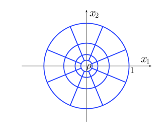
Figure 3: A typical mesh $\mathscr{T}_{h}$ with $N=8$.

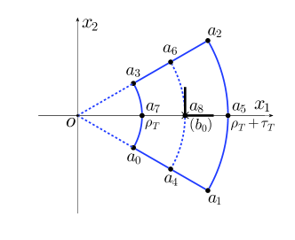
Figure 4: A circular ring sector element $T$.

In our numerical experiments, the number of elements $N$ in the circular ring layers and the thickness $\tau_{T}$ of each layer are determined by a meshing strategy based on an energy equi-distribution principle established in [9]. For given $\rho>0$, the meshes so produced satisfy the mesh regularity conditions (M1) and (M2). Table 1 shows two sets of typical meshes produced by the meshing strategy. For the constant $\sigma$ in (C1), we set $\sigma=\rho/C_{max}$, where $C_{max}$ is an upper bound for the expected grown cavity radius. In our numerical experiments, we set $\sigma=\rho/2$, i.e. $C_{max}=2$.

$h$	$\min\tau_{T}$	$\max\tau_{T}$	layers	$N$
0.05	0.0300	0.1900	8	20
0.04	0.0224	0.1376	11	26
0.03	0.0156	0.1164	14	34
0.02	0.0096	0.0736	22	50

(a) $\rho=0.01$.

$h$	$\min\tau_{T}$	$\max\tau_{T}$	layers	$N$
0.05	0.0120	0.1720	9	24
0.04	0.0080	0.1360	12	28
0.03	0.0048	0.1056	16	38
0.02	0.0024	0.0728	22	56

(b) $\rho=0.0001$.

Table 1: Data of two sets of typical meshes produced.

3.1 Radially symmetric case

In our numerical experiments, we take $\bm{u}(\bm{x};\lambda)=\frac{\sqrt{R^{2}+\lambda^{2}-1}}{R}\bm{x}$ with $\lambda>1$ as the analytical cavitation solution to the radially symmetric dead-load traction problem with

$$\bm{t}(\bm{x})=t\bm{n}(\bm{x}),\;\;\forall\bm{x}\in\partial B_{1}(\bm{0}),\quad\;\text{and}\quad\;\bm{t}(\bm{x})=\bm{0},\;\;\forall\bm{x}\in\partial B_{\rho}(\bm{0}),$$ (3.2)

where $\bm{n}$ is the unit outward normal to $\partial B_{1}(\bm{0})$, and $t=t_{\rho,\lambda}$ is uniquely determined by $\rho$ and $\lambda$ [3]. For example $t_{0.1,2}\approx 3.00487$, $t_{0.01,2}\approx 3.94237$, $t_{0.0001,2}\approx 4.21590$.

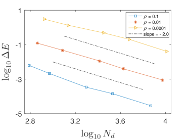
(a) Energy error $\Delta E=|E(\bm{u}_{h})-E(\bm{u})|$.

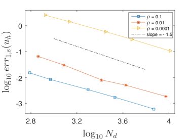
(b) Error in $W^{1,s}$-seminorm $|\bm{u}_{h}-\bm{u}|_{1,s,\Omega}$.

Figure 5: Convergence behavior of the energy and deformation in symmetric case.

The convergence behavior of the numerical cavitation solutions with $\lambda=2$ obtained by the DP-Q2-P1 mixed finite element method is shown in Fig 5-Fig 8, where $N_{d}$ is the total degrees of freedom of $\bm{u}_{h}$. Fig 8 shows $N_{d}$ as a function of the mesh size $h$ in the radially symmetric case. It is clearly seen that $N_{d}\sim h^{-2}$ for our mesh and the convergence rates obtained by the DP-Q2-P1 cavitation solutions in the radially symmetric case can reach the optimal rates of the interpolation error estimates, which were analyzed in [9] (see Theorem 5.2 in [9]).

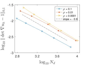
(a) $L^{1}$ error of $\det\nabla u_{h}$.

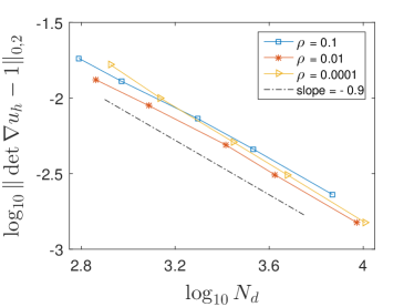
(b) $L^{2}$ error of $\det\nabla u_{h}$.

Figure 6: Convergence behavior of $\det\nabla u_{h}$ in symmetric case.

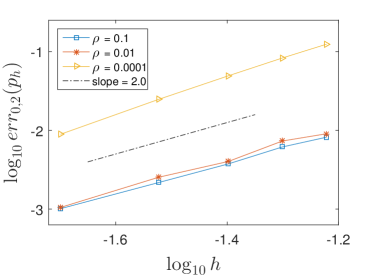
Figure 7: Convergence behavior of $p_{h}$.

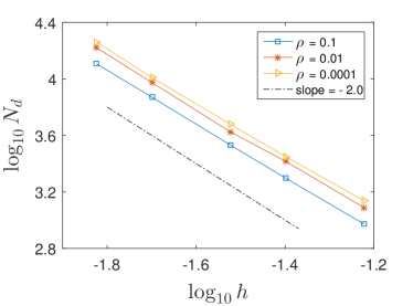
Figure 8: $N_{d}\sim h^{-2}$ in symmetric case.

3.2 Non-radially symmetric case

Consider the non-radially-symmetric dead-load traction problem with

$$\bm{t}(\bm{x})=(1+\eta|\cos\theta|)t\bm{n}(\bm{x}),\;\;\forall\bm{x}\in\partial B_{1}(\bm{0}),\quad\;\text{and}\quad\;\bm{t}(\bm{x})=\bm{0},\;\;\forall\bm{x}\in\partial B_{\rho}(\bm{0}),$$ (3.3)

where $\theta=\arctan(x_{2}/x_{1})$, $\eta$ and $t$ are parameters. In our numerical experiments, we take $\eta=1/10$, and $t=t_{\rho,2}$ as is given in the radially-symmetric case for various $\rho$.

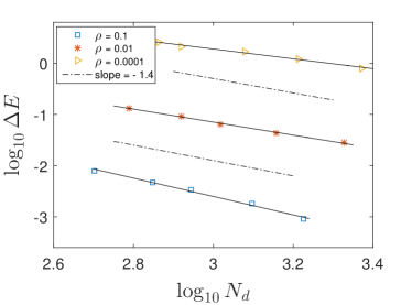
(a) Energy error $\Delta E=|E(\bm{u}_{h})-E(\bm{u})|$.

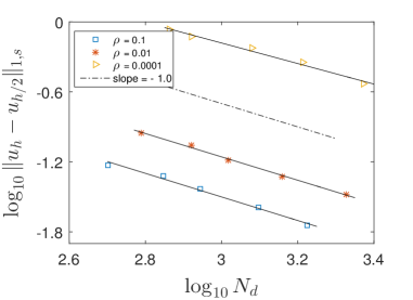
(b) Error in $W^{1,s}$-seminorm $|\bm{u}_{h}-\bm{u}|_{1,s,\Omega}$.

Figure 9: Convergence behavior of the energy and deformation in non-symmetric case.

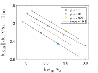
(a) $L^{1}$ error of $\det\nabla u_{h}$.

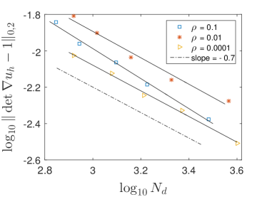
(b) $L^{2}$ error of $\det\nabla u_{h}$.

Figure 10: Convergence behavior of $\det\nabla u_{h}$ in non-symmetric case.

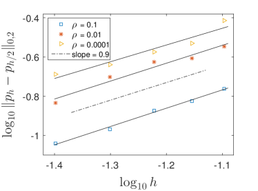
Figure 11: Convergence behavior of $p_{h}$.

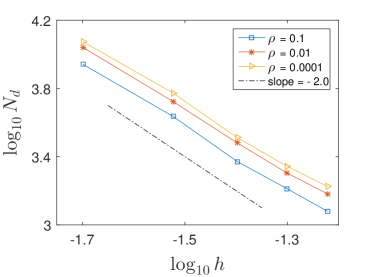
Figure 12: $N_{d}\sim h^{-2}$ in non-symmetric case.

The convergence behavior of the numerical cavitation solutions obtained by the DP-Q2-P1 mixed finite element method is shown in Fig 9-Fig 12. Fig 12 shows $N_{d}$ as a function of $h$ in the non-radially-symmetric case. We see that, in the non-radially-symmetric case, again $N_{d}\sim h^{-2}$ for the meshes produced by the meshing strategy, and the convergence rates obtained by the DP-Q2-P1 cavitation solutions, though dropped a little bit, are still close to the optimal rates (see [9]).

4 Conclusion

A DP-Q2-P1 mixed finite element method combined with a damped Newton iteration scheme is established in this paper to numerically solve large deformation problems in incompressible nonlinear elasticity. The method is analytically proved to be locking-free and stable. The numerical experiments on some typical cavitation problems demonstrate the accuracy and efficiency of the method in solving incompressible nonlinear elasticity problems with extremely large anisotropic deformation gradients.

References

[1] Kouhia, R., Stenberg, R., A linear nonconforming finite element
method for nearly incompressible elasticity and Stokes flow.
Comput. Methods Appl. Mech. Engrg., 124 (1995), 195-212.
[2] Dobrowolski, M., A mixed finite element method for approximating
incompressible materials. SIAM J. Numer. Anal., 29 (1992), 365-389.
[3] Ball, J. M., Discontinuous equilibrium solutions and cavitation in
nonlinear elasticity. Philos. Trans. R. Soc. London, A 306 (1982),
557-611.
[4] Ball, J. M. and James, R. D., Fine phase mixtures
as minimizers of energy. Arch. Rat. Mech. Anal., 100(1)(1987), 13-52.
[5] Müller, S., Spector S. J., An existence theory for nonlinear
elasticity that allows for cavitation. Arch. Rat.
Mech. Anal., 131 (1995), 1-66.
[6] Lian, Y., Li, Z., A dual-parametric finite element method
for cavitation in nonlinear elasticity. J. Comput. Appl. Math.,
236 (2011), 834-842.
[7] Xu, X., Henao, D., An efficient numerical method for
cavitation in nonlinear elasticity. Math. Models Methods Appl. Sci., 21
(2011), 1733-1760.
[8] Hardik K., Adrian J. L. and Cockburn B., A hybridizable discontinuous
Galerkin formulation for nonlinear elasticity. Comput. Methods Appl. Mech. Engrg.,
283 (2015), 303-329.
[9] Su, C., Li, Z., Error analysis of a dual-parametric bi-quadratic
FEM in cavitation computation in elasticity. SIAM J. Numer. Anal., 53(3)
(2015), 1629-1649.
[10] Li, Z., A numerical method for computing singular minimizers.
Numer. Math., 71 (1995), 317-330.
[11] Brezzi, F., Fortin, M., Mixed and hybrid finite element methods.
Springer-Verlag, New York (1991).
[12] John D., Ted B., Volumetric locking in the element free
Galerkin method. Int. J. Numer. Meth. Engng., 46 (1999), 925-942.
[13] Rohan, P. Y., Lobos, C., Nazari, M. A., Perrier, P., Payan, Y.,
Finite element modelling of nearly incompressible materials and volumetric locking:
a case study. Comput. Methods Biomech. Biomed. Eng., 17 (sup1) (2014), 192-193.
[14] Girault. V., Raviart. P.-A., Finite element methods
for navier-stokes equations: theorey and algorithms.
Springer-Verlag, Berlin Heidelberg New York (1986).
[15] Nirenberg, L., On elliptic partial differential equations.
Ann. Scuola Norm. Sup. Pisa Sci. Fis. Mat., 13 (1959), 116-162.
[16] Simo, J. C., Rifai, M. S., A class of mixed assumed strain methods
and the method of incompatible modes. Int. J. Numer. Methods Engrg., 29(8)
(1990), 1595-1638.
[17] Chavan, K. S., Lamichhane, B. P., Wohlmuth, B. I.,
Locking-free finite element methods for linear and nonlinear elasticity
in 2D and 3D. Comput. Methods Appl. Mech. Engrg, 196(41) (2007), 4075-4086.
[18] Braess, D., Ming, P., A finite element method for nearly
incompressible elasticity problems. Math. Comput., 74(249) (2005), 25-52.