Revisiting the Design Issues of Local Models for
Japanese Predicate-Argument Structure Analysis

Abstract

The research trend in Japanese predicate-argument structure (PAS) analysis is shifting from pointwise prediction models with local features to global models designed to search for globally optimal solutions. However, the existing global models tend to employ only relatively simple local features; therefore, the overall performance gains are rather limited. The importance of designing a local model is demonstrated in this study by showing that the performance of a sophisticated local model can be considerably improved with recent feature embedding methods and a feature combination learning based on a neural network, outperforming the state-of-the-art global models in $F_{1}$ on a common benchmark dataset.

1 Introduction

A predicate-argument structure (PAS) analysis is the task of analyzing the structural relations between a predicate and its arguments in a text and is considered as a useful sub-process for a wide range of natural language processing applications Shen and Lapata (2007); Kudo et al. (2014); Liu et al. (2015).

PAS analysis can be decomposed into a set of primitive subtasks that seek a filler token for each argument slot of each predicate. The existing models for PAS analysis fall into two types: local models and global models. Local models independently solve each primitive subtask in the pointwise fashion Seki et al. (2002); Taira et al. (2008); Imamura et al. (2009); Yoshino et al. (2013). Such models tend to be easy to implement and faster compared with global models but cannot handle dependencies between primitive subtasks. Recently, the research trend is shifting toward global models that search for a globally optimal solution for a given set of subtasks by extending those local models with an additional ranker or classifier that accounts for dependencies between subtasks Iida et al. (2007a); Komachi et al. (2010); Yoshikawa et al. (2011); Hayashibe et al. (2014); Ouchi et al. (2015); Iida et al. (2015, 2016); Shibata et al. (2016).

However, even with the latest state-of-the-art global models Ouchi et al. (2015, 2017), the best achieved $F_{1}$ remains as low as $81.4\%$ on a commonly used benchmark dataset Iida et al. (2007b), wherein the gain from the global scoring is only 0.3 to 1.0 point. We speculate that one reason for this slow advance is that recent studies pay too much attention to global models and thus tend to employ overly simple feature sets for their base local models.

The goal of this study is to argue the importance of designing a sophisticated local model before exploring global solution algorithms and to demonstrate its impact on the overall performance through an extensive empirical evaluation. In this evaluation, we show that a local model alone is able to significantly outperform the state-of-the-art global models by incorporating a broad range of local features proposed in the literature and training a neural network for combining them. Our best local model achieved $13$% error reduction in $F_{1}$ compared with the state of the art.

2 Task and Dataset

In this study, we adopt the specifications of the NAIST Text Corpus (NTC) Iida et al. (2007b), a commonly used benchmark corpus annotated with nominative (NOM), accusative (ACC), and dative (DAT) arguments for predicates. Given an input text and the predicate positions, the aim of the PAS analysis is to identify the head of the filler tokens for each argument slot of each predicate.

The difficulty of finding an argument tends to differ depending on the relative position of the argument filler and the predicate. In particular, if the argument is omitted and the corresponding filler appears outside the sentence, the task is much more difficult because we cannot use the syntactic relationship between the predicate and the filler in a naive way. For this reason, a large part of previous work narrowed the focus to the analysis of arguments in a target sentence Yoshikawa et al. (2011); Ouchi et al. (2015); Iida et al. (2015), and here, we followed this setting as well.

3 Model

Given a tokenized sentence $s$ and a target predicate $p$ in $s$ with the gold dependency tree $t$, the goal of our task is to select at most one argument token $\hat{a}$ for each case slot of the target predicate.

Taking $x_{a}=(a,p,s,t)$ as input, our model estimates the probability $p(c|x_{a})$ of assigning a case label $c\in\{\mathtt{NOM},\mathtt{ACC},\mathtt{DAT},\mathtt{NONE}\}$ for each token $a$ in the sentence, and then selects a token with a maximum probability that exceeds the output threshold $\theta_{c}$ for $c$. The probability $p(c|x_{a})$ is modeled by a neural network (NN) architecture, which is a fully connected multilayer feedforward network stacked with a softmax layer on the top (Figure 1).

$$g = \mathrm{softmax}(W_{n+1}h_{n}+b_{n+1})$$ (1)

$$h_{i} = \mathrm{ReLU}(\mathrm{BN}(W_{i}h_{i-1}+b_{i}))$$ (2)

$$h_{1} = \mathrm{ReLU}(\mathrm{BN}(W_{1}m+b_{1}))$$ (3)

$$m = [h_{\rm path},w_{p},w_{a},f(x_{a})]$$ (4)

The network outputs the probabilities $g$ of assigning each case label for an input token $a$, from automatically learned combinations of feature representations in input $m$. Here, $h_{i}$ is an $i$-th hidden layer and $n$ is the number of hidden layers. We apply batch normalization (BN) and a ReLU activation function to each hidden layer.

The input layer $m$ for the feedforward network is a concatenation of the three types of feature representations described below: a path embedding $h_{\rm path}$, word embeddings of the predicate and the argument candidate $w_{p}$ and $w_{a}$, and a traditional binary representation of other features $f(x_{a})$.

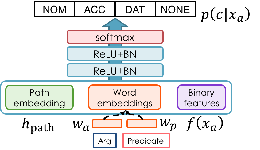
Figure 1: Network structure of our NN model

3.1 Lexicalized path embeddings

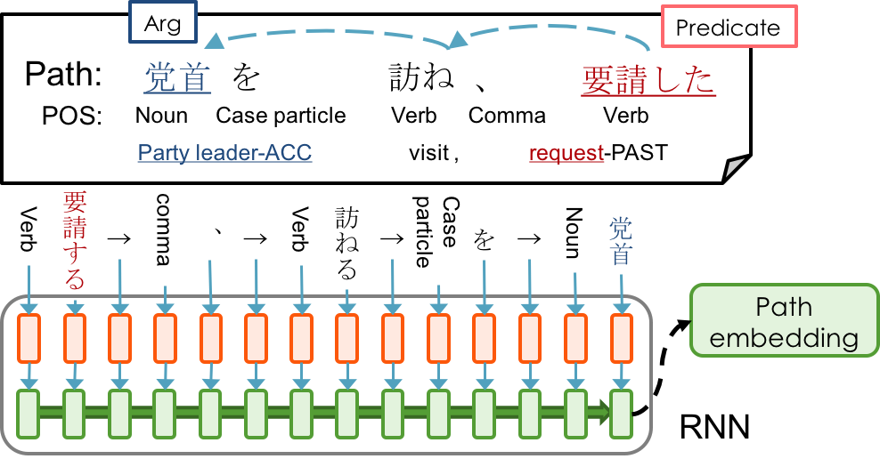
Figure 2: Path embedding

When an argument is not a direct dependent of a predicate, the dependency path is considered as important information. Moreover, in some constructions such as raising, control, and coordination, lexical information of intermediate nodes is also beneficial although a sparsity problem occurs with a conventional binary encoding of lexicalized paths.

Roth and Lapata (2016) and Shwartz et al. (2016) recently proposed methods for embedding a lexicalized version of dependency path on a single vector using RNN. Both the methods embed words, parts-of-speech, and directions and labels of dependency in the path into a hidden unit of LSTM and output the final state of the hidden unit. We adopt these methods for Japanese PAS analysis and compare their performances.

As shown in Figure 2, given a dependency path from a predicate to an argument candidate, we first create a sequence of POS, lemma, and dependency direction for each token in this order by traversing the path. Next, an embedding layer transforms the elements of this sequence into vector representations. The resulting vectors are sequentially input to RNN. Then, we use the final hidden state as the path-embedding vector. We employ GRU Cho et al. (2014) for our RNN and use two types of input vectors: the adaptations of Roth and Lapata (2016), which we described in Figure 2, and Shwartz et al. (2016), which concatenates vectors of POS, lemma and dependency direction for each token into a single vector.

3.2 Word embedding

The generalization of a word representation is one of the major issues in SRL. Fitzgerald et al. (2015) and Shibata et al. (2016) successfully improved the classification accuracy of SRL tasks by generalizing words using embedding techniques. We employ the same approach as Shibata et al. (2016), which uses the concatenation of the embedding vectors of a predicate and an argument candidate.

For	surface, lemma, POS,
predicate	type of conjugated form,
$p$	nominal form of nominal verb,
	voice suffixes (-reru, -seru, -dekiru, -tearu)
For	surface, lemma, POS, NE tag,
argument	whether $a$ is head of bunsetsu,
candidate	particles in bunsetsu,
$a$	right neighbor token’s lemma and POS
Between	case markers of other dependents of $p$,
predicate	whether $a$ precedes $p$,
and	whether $a$ and $p$ are in the same bunsetsu,
argument	token- and dependency-based distances,
candidate	naive dependency path sequence

Table 1: Binary features

3.3 Binary features

Case markers of the other dependents

Our model independently estimates label scores for each argument candidate. However, as argued by Toutanova et al. (2008) and Yoshikawa et al. (2011), there is a dependency between the argument labels of a predicate.

In Japanese, case markers (case particles) partially represent a semantic relationship between words in direct dependency. We thus introduce a new feature that approximates co-occurrence bias of argument labels by gathering case particles for the other direct dependents of a target predicate.

Other binary features

The other binary features employed in our models have mostly been discussed in previous work Imamura et al. (2009); Hayashibe et al. (2011). The entire list of our binary features are presented in Table 1.

4 Experiments

		All			$F_{1}$ in different dependency distance
Model	Binary feats.	$F_{1}$ ($\sigma$)	Prec.	Rec.	Dep	Zero	2	3	4	$\geq$ 5
B	all	82.02 ($\pm$0.13)	83.45	80.64	89.11	49.59	57.97	47.2	37	21
B	$-$cases	81.64 ($\pm$0.19)	83.88	79.52	88.77	48.04	56.60	45.0	36	21
WB	all	82.40 ($\pm$0.20)	85.30	79.70	89.26	49.93	58.14	47.4	36	23
WBP-Roth	all	82.43 ($\pm$0.15)	84.87	80.13	89.46	50.89	58.63	49.4	39	24
WBP-Shwartz	all	83.26 ($\pm$0.13)	85.51	81.13	89.88	51.86	60.29	49.0	39	22
WBP-Shwartz	$-$word	83.23 ($\pm$0.11)	85.77	80.84	89.82	51.76	60.33	49.3	38	21
WBP-Shwartz	$-${word, path}	83.28 ($\pm$0.16)	85.77	80.93	89.89	51.79	60.17	49.4	38	23
WBP-Shwartz (ens)	$-${word, path}	83.85	85.87	81.93	90.24	53.66	61.94	51.8	40	24
WBP-Roth	$-${word, path}	82.26 ($\pm$0.12)	84.77	79.90	89.28	50.15	57.72	49.1	38	24
BP-Roth	$-${word, path}	82.03 ($\pm$0.19)	84.02	80.14	89.07	49.04	57.56	46.9	34	18
WB	$-${word, path}	82.05 ($\pm$0.19)	85.42	78.95	89.18	47.21	55.42	43.9	34	21
B	$-${word, path}	78.54 ($\pm$0.12)	79.48	77.63	85.59	40.97	49.96	36.8	22	9.1

Table 2: Impact of each feature representation. “$-$ word” indicates the removal of surface and lemma features. “$-$ cases” and “$-$ path” indicate the removal of the case markers of other dependents and binary path features, respectively. The task Zero is equivalent to the cases where the dependency distance $\geq 2$.

4.1 Experimental details

Dataset

The experiments were performed on the NTC corpus v1.5, dividing it into commonly used training, development, and test divisions Taira et al. (2008).

Hyperparameters

We chose the hyperparameters of our models to obtain a maximum score in $F_{1}$ on the development data. We select $2,000$ for the dimension of the hidden layers in the feedforward network from $\{256,512,1000,2000,3000\}$, $2$ for the number of hidden layers from $\{1,2,3,4\}$, $192$ for the dimension of the hidden unit in GRU from $\{32,64,128,192\}$, $0.2$ for the dropout rate of GRUs from $\{0.0,0.1,0.2,0.3,0.5\}$, and $128$ for the mini-batch size on training from $\{32,64,128\}$.

We employed a categorical cross-entropy loss for training, and used Adam with $\beta_{1}=0.9$, $\beta_{2}=0.999$, and $\epsilon=1e-08$. The learning rate for each model was set to $0.0005$. All the model were trained with early stopping method with a maximum epoch number of 100, and training was terminated after five epochs of unimproved loss on the development data. The output thresholds for case labels were optimized on the training data.

Initialization

All the weight matrices in GRU were initialized with random orthonormal matrices. The word embedding vectors were initialized with 256-dimensional Word2Vec vectors trained on the entire Japanese Wikipedia articles dumped on September 1st, 2016. We extracted the body texts using WikiExtractor, and tokenized them using the CaboCha dependency parser v0.68 with JUMAN dictionary. The vectors were trained on lemmatized texts. Adjacent verbal noun and light verb were combined in advance. Low-frequent words appearing less than five times were replaced by their POS, and we used trained POS vectors for words that were not contained in a lexicon of Wikipedia word vectors in the PAS analysis task.

We used another set of word/POS embedding vectors for lexicalized path embeddings, initialized with 64-dimensional Word2Vec vectors. The embeddings for dependency directions were randomly initialized. All the pre-trained embedding vectors were fine-tuned in the PAS analysis task.

The hyperparameters for Word2Vec are “-cbow 1 -window 10 -negative 10 -hs 0 -sample 1e-5 -threads 40 -binary 0 -iter 3 -min-count 10”.

Preprocessing

We employed a common experimental setting that we had an access to the gold syntactic information, including morpheme segmentations, parts-of-speech, and dependency relations between bunsetsus. However, instead of using the gold syntactic information in NTC, we used the output of CaboCha v0.68 as our input to produce the same word segmentations as in the processed Wikipedia articles. Note that the training data for the parser contain the same document set as in NTC v1.5, and therefore, the parsing accuracy for NTC was reasonably high.

The binary features appearing less than 10 times in the training data were discarded. For a path sequence, we skipped a middle part of intermediate tokens and inserted a special symbol in the center of the sequence if the token length exceeded 15.

4.2 Results

In the experiment, in order to examine the impact of each feature representation, we prepare arbitrary combinations of word embedding, path embedding, and binary features, and we use them as input to the feedforward network. For each model name, W, P, and B indicate the use of word embedding, path embedding, and binary features, respectively. In order to compare the performance of binary features and embedding representations, we also prepare multiple sets of binary features. The evaluations are performed by comparing precision, recall, and $F_{1}$ on the test set. These values are the means of five different models trained with the same training data and hyperparameters.

		Dep				Zero
Model	ALL	ALL	NOM	ACC	DAT	ALL	NOM	ACC	DAT
On NTC 1.5
WBP-Shwartz (ens) $-${word, path}	83.85	90.24	91.59	95.29	62.61	53.66	56.47	44.7	16
B	82.02	89.11	90.45	94.61	60.91	49.59	52.73	38.3	11
Ouchi et al. (2015)-local	78.15	85.06	86.50	92.84	30.97	41.65	45.56	21.4	0.8
Ouchi et al. (2015)-global	79.23	86.07	88.13	92.74	38.39	44.09	48.11	24.4	4.8
Ouchi et al. (2017)-multi-seq	81.42	88.17	88.75	93.68	64.38	47.12	50.65	32.4	7.5
Subject anaphora resolution on modified NTC, cited from Iida et al. (2016)
Ouchi et al. (2015)-global							57.3
Iida et al. (2015)							41.1
Iida et al. (2016)							52.5

Table 3: Comparisons to previous work in $F_{1}$

Impact of feature representations

The first row group in Table 2 shows the impact of the case markers of the other dependents feature. Compared with the model using all the binary features, the model without this feature drops by $0.3$ point in $F_{1}$ for directly dependent arguments (Dep), and $1.6$ points for indirectly dependent arguments (Zero). The result shows that this information significantly improves the prediction in both Dep and Zero cases, especially on Zero argument detection.

The second row group compares the impact of lexicalized path embeddings of two different types. In our setting, WBP-Roth and WB compete in overall $F_{1}$, whereas WBP-Roth is particularly effective for Zero. WBP-Shwartz obtains better result compared with WBP-Roth, with further $0.9$ point increase in comparison to the WB model. Moreover, its performance remains without lexical and path binary features. The WBP-Shwartz (ens)$-${word, path} model, which is the ensemble of the five WBP-Shwartz$-${word, path} models achieves the best $F_{1}$ score of $83.85\%$.

To highlight the role of word embedding and path embedding, we compare B, WB, BP-Roth, and WBP-Roth models on the third row group, without using lexical and path binary features. When we respectively remove W and P-Roth from WBP-Roth, then the performance decreases by $0.23$ and $0.21$ in $F_{1}$. Roth and Lapata (2016) reported that $F_{1}$ decreased by 10 points or more when path embedding was excluded. However, in our models, such a big decline occurs when we omit both path and word embeddings. This result suggests that the word inputs at both ends of the path embedding overlap with the word embedding and the additional effect of the path embedding is rather limited.

Comparison to related work

Table 3 shows the comparison of $F_{1}$ with existing research. First, among our models, the B model that uses only binary features already outperforms the state-of-the-art global model on NTC 1.5 Ouchi et al. (2017) in overall $F_{1}$ with $0.6$ point of improvement. Moreover, the B model outperforms the global model of Ouchi et al. (2015) that utilizes the basic feature set hand-crafted by Imamura et al. (2009) and Hayashibe et al. (2011) and thus contains almost the same binary features as ours. These results show that fine feature combinations learned by deep NN contributes significantly to the performance. The WBP-Shwartz (ens)$-${word, path} model, which has the highest performance among our models shows a further $1.8$ points improvement in overall $F_{1}$, which achieves $13$% error reduction compared with the state-of-the-art grobal model ($81.42$% of Ouchi et al. (2017)-multi-seq).

Iida et al. (2015) and Iida et al. (2016) tackled the task of Japanese subject anaphora resolution, which roughly corresponds to the task of detecting Zero NOM arguments in our task. Although we cannot directly compare the results with their models due to the different experimental setup, we can indirectly see our model’s superiority through the report on Iida et al. (2016), wherein the replication of Ouchi et al. (2015) showed 57.3% in $F_{1}$, whereas Iida et al. (2015) and Iida et al. (2016) gave 41.1% and 52.5%, respectively.

As a closely related work to ours, Shibata et al. (2016) adapted a NN framework to the model of Ouchi et al. (2015) using a feedforward network for calculating the score of the PAS graph. However, the model is evaluated on a dataset annotated with a different semantics; therefore, it is difficult to directly compare the results with ours.

Unfortunately, in the present situation, a comprehensive comparison with a broad range of prior studies in this field is quite difficult for many historical reasons (e.g., different datasets, annotation schemata, subtasks, and their own preprocesses or modifications to the dataset). Creating resources that would enable a fair and comprehensive comparison is one of the important issues in this field.

5 Conclusion

This study has argued the importance of designing a sophisticated local model before exploring global solution algorithms in Japanese PAS analysis and empirically demonstrated that a sophisticated local model alone can outperform the state-of-the-art global model with $13$% error reduction in $F_{1}$. This should not be viewed as a matter of local models vs. global models. Instead, global models are expected to improve the performance by incorporating such a strong local model.

In addition, the local features that we employed in this paper is only a part of those proposed in the literature. For example, selectional preference between a predicate and arguments is one of the effective information Sasano and Kurohashi (2011); Shibata et al. (2016), and local models could further improve by combining these extra features.

References

- Cho et al. (2014) Kyunghyun Cho, Bart Van Merrienboer, Dzmitry Bahdanau, and Yoshua Bengio. 2014. On the Properties of Neural Machine Translation : Encoder â Decoder Approaches. In SSST-8, pages 103–111.
- Fitzgerald et al. (2015) Nicholas Fitzgerald, Oscar Täckström, Kuzman Ganchev, and Dipanjan Das. 2015. Semantic Role Labeling with Neural Network Factors. In EMNLP, pages 960–970.
- Hayashibe et al. (2011) Yuta Hayashibe, Mamoru Komachi, and Yuji Matsumoto. 2011. Japanese Predicate Argument Structure Analysis Exploiting Argument Position and Type. In IJCNLP, pages 201–209.
- Hayashibe et al. (2014) Yuta Hayashibe, Mamoru Komachi, and Yuji Matsumoto. 2014. Japanese Predicate Argument Structure Analysis by Comparing Candidates in Different Positional Relations between Predicate and Arguments. Journal of Natural Language Processing, 21(1):3–25.
- Iida et al. (2007a) Ryu Iida, Kentaro Inui, and Yuji Matsumoto. 2007a. Zero-anaphora resolution by learning rich syntactic pattern features. Transactions on Asian and Low-Resource Language Information Processing, 6(4):1–22.
- Iida et al. (2007b) Ryu Iida, Mamoru Komachi, Kentaro Inui, and Yuji Matsumoto. 2007b. Annotating a Japanese Text Corpus with Predicate-Argument and Coreference Relations. In Linguistic Annotation Workshop, pages 132–139.
- Iida et al. (2015) Ryu Iida, Kentaro Torisawa, Chikara Hashimoto, Jong-Hoon Oh, and Julien Kloetzer. 2015. Intra-sentential Zero Anaphora Resolution using Subject Sharing Recognition. In EMNLP, pages 2179–2189.
- Iida et al. (2016) Ryu Iida, Kentaro Torisawa, Jong-Hoon Oh, Canasai Kruengkrai, and Julien Kloetzer. 2016. Intra-Sentential Subject Zero Anaphora Resolution using Multi-Column Convolutional Neural Network. In EMNLP, pages 1244–1254.
- Imamura et al. (2009) Kenji Imamura, Kuniko Saito, and Tomoko Izumi. 2009. Discriminative Approach to Predicate-Argument Structure Analysis with Zero-Anaphora Resolution. In ACL-IJCNLP, pages 85–88.
- Komachi et al. (2010) Mamoru Komachi, Ryu Iida, Kentaro Inui, and Yuji Matsumoto. 2010. Argument structure analysis of event-nouns using lexico-syntactic patterns of noun phrases. Journal of Natural Language Processing, 17(1):141–159.
- Kudo et al. (2014) Taku Kudo, Hiroshi Ichikawa, and Hideto Kazawa. 2014. A Joint Inference of Deep Case Analysis and Zero Subject Generation for Japanese-to-English Statistical Machine Translation. In ACL, pages 557–562.
- Liu et al. (2015) Fei Liu, Jeffrey Flanigan, Sam Thomson, Norman Sadeh, and Noah A. Smith. 2015. Toward Abstractive Summarization Using Semantic Representations. In NAACL, pages 1076–1085.
- Ouchi et al. (2015) Hiroki Ouchi, Hiroyuki Shindo, Kevin Duh, and Yuji Matsumoto. 2015. Joint Case Argument Identification for Japanese Predicate Argument Structure Analysis. In ACL-IJCNLP, pages 961–970.
- Ouchi et al. (2017) Hiroki Ouchi, Hiroyuki Shindo, and Yuji Matsumoto. 2017. Neural Modeling of Multi-Predicate Interactions for Japanese Predicate Argument Structure Analysis. In ACL, pages 1591–1600.
- Roth and Lapata (2016) Michael Roth and Mirella Lapata. 2016. Neural Semantic Role Labeling with Dependency Path Embeddings. In ACL, pages 1192–1202.
- Sasano and Kurohashi (2011) Ryohei Sasano and Sadao Kurohashi. 2011. A Discriminative Approach to Japanese Zero Anaphora Resolution with Large-scale Lexicalized Case Frames. In IJCNLP, pages 758–766.
- Seki et al. (2002) Kazuhiro Seki, Atsushi Fujii, and Tetsuya Ishikawa. 2002. A Probabilistic Method for Analyzing Japanese Anaphora Integrating Zero Pronoun Detection and Resolution. In COLING, pages 911â–917.
- Shen and Lapata (2007) Dan Shen and Mirella Lapata. 2007. Using Semantic Roles to Improve Question Answering. In EMNLP-CoNLL, pages 12–21.
- Shibata et al. (2016) Tomohide Shibata, Daisuke Kawahara, and Sadao Kurohashi. 2016. Neural Network-Based Model for Japanese Predicate Argument Structure Analysis. In ACL, pages 1235–1244.
- Shwartz et al. (2016) Vered Shwartz, Yoav Goldberg, and Ido Dagan. 2016. Improving Hypernymy Detection with an Integrated Pattern-based and Distributional Method. In ACL, pages 2389–2398.
- Taira et al. (2008) Hirotoshi Taira, Sanae Fujita, and Masaaki Nagata. 2008. A Japanese Predicate Argument Structure Analysis using Decision Lists. In EMNLP, pages 523–532.
- Toutanova et al. (2008) Kristina Toutanova, Aria Haghighi, and Christopher D Manning. 2008. A Global Joint Model for Semantic Role Labeling. Computational Linguistics, 34(2):161–191.
- Yoshikawa et al. (2011) Katsumasa Yoshikawa, Masayuki Asahara, and Yuji Matsumoto. 2011. Jointly Extracting Japanese Predicate-Argument Relation with Markov Logic. In IJCNLP, pages 1125–1133.
- Yoshino et al. (2013) Koichiro Yoshino, Shinsuke Mori, and Tatsuya Kawahara. 2013. Predicate Argument Structure Analysis using Partially Annotated Corpora. In IJCNLP, pages 957–961.