Simulating Dirac models with ultracold atoms in optical lattices

Abstract

We present a general model allowing “quantum simulation” of one-dimensional Dirac models with 2- and 4-component spinors using ultracold atoms in driven 1D tilted optical latices. The resulting Dirac physics is illustrated by one of its well-known manifestations, Zitterbewegung. This general model can be extended and applied with great flexibility to more complex situations.

I Introduction

The Dirac theory of the electron (with its quantum-electrodynamical corrections) is the most complete, precise, and experimentally well-tested theory in physics. It combines quantum mechanics and relativistic covariance in a general frame, automatically including the spin degree of freedom, and predicting the existence of the positron. However, in atomic physics, and a fortiori in cold-atom physics, Dirac theory has played a relatively restricted role, because, experimentally, its domain of application ($v\sim c$) is not often attained (except for inner-shell electrons of heavy atoms) and, theoretically, many of its important results (e.g. fine structure) can be calculated with a good precision in the simpler frame of Pauli theory (that is, Schrödinger equation plus spin 1/2), at least for light atoms.

Recently, quantum simulation (Georgescu et al., 2014) became a mainstream in ultracold-atom physics (Bloch et al., 2014). The basic idea, inspired by early Feynman insights (Feynman, 1982), is to generate the physical behavior corresponding to some model, e.g. condensed matter’s Hubbard Hamiltonians, by “artificially” creating a corresponding Hamiltonian in more controlled conditions, e.g. ultracold atoms in optical lattices (Bloch et al., 2008). This “Hamiltonian engineering” has been pushed quite far, with the introduction of artificial gauge fields (Dalibard et al., 2011), spin-orbit couplings and Dirac equation simulations Gerritsma et al. (2010); Witthaut et al. (2011); Salger et al. (2011); Galitski and Spielman (2013), quantum magnetism of neutral atoms (Lin et al., 2009; Struck et al., 2012), and the physics of disordered systems (Chabé et al., 2008; Billy et al., 2008; Roati et al., 2008; Kondov et al., 2011; Manai et al., 2015).

Quantum simulation of Dirac physics has benefit of a large interest in recent years. This can be done in condensed matter systems by taking advantage of the flexible concept of quasi-particles, where in particular the Weyl semimetal Wang et al. (2017) is a pertinent concept, and recently the existence of “type-II” Weyl particles (that is a Weyl particle breaking Lorentz isotropy) Soluyanov et al. (2017) has been suggested. Dirac quantum simulators using ion traps have also been proposed Lamata et al. (2011). Another popular way of quantum-simulating Dirac physics is by using ultracold atoms in optical lattices, pioneered by Gerritsma et al. Gerritsma et al. (2010, 2011), who studied the phenomenon of Klein tunneling, also studied in refs. Salger et al. (2011); Witthaut et al. (2011); Suchet et al. (2016). Without trying to be exhaustive, a wealth of interesting related phenomena can also be studied: topological insulators, Dirac cones, spin-orbit coupling, and even cyclotron dynamics Mazza et al. (2012); Kolovsky and Bulgakov (2013); Tarruell et al. (2012); Lopez-Gonzalez et al. (2014); Jiménez-García et al. (2015); Zhang et al. (2012); Kolovsky (2012).

The present work combines these two driving forces in the ultracold-atom field. We propose a general method for simulating Dirac physics in a “tilted” one-dimensional optical lattice, a system that has been very useful since the early days of the quantum simulation (even before the term quantum simulation was introduced), for example for the observation of Bloch oscillations or the (equivalent) Wannier-Stark ladder Ben Dahan et al. (1996); Niu et al. (1996); Kolovsky et al. (2010, 2009); Glück et al. (2000, 1999, 2002). The realization of such a system can be obtained by applying a far-detuned laser standing wave that ultracold atoms see as a sinusoidal potential acting on their center of mass variables (Cohen-Tannoudji and Guéry-Odelin, 2011). If the atom’s de Broglie wavelength is comparable to the lattice constant $\mathsf{a}=\lambda_{L}/2$, where $\lambda_{L}=2\pi/k_{L}$ is the radiation wavelength (we use sans serif symbols for dimensioned quantities), the system is in the quantum regime, a condition easily realized for temperatures of the order of a few $\mu$K. In order to obtain a tilted potential, one can simply chirp one of the beams forming the standing wave: A linear shift of the frequency produces a quadratic displacement of the nodes of the standing wave; in the rest frame with respect to the nodes, an inertial constant force creates a tilt, that is, a potential of the form $\mathsf{V}_{ws}(\mathsf{x})=-\mathsf{V}_{1}\cos(2k_{L}\mathit{\mathsf{x}})+\mathsf{Fx}$, with $\mathsf{V}_{1}$ proportional to the radiation intensity and $\mathsf{F}$ (constant) proportional to the frequency chirp. This kind of setup is by now quite common in cold atom physics. In what follows, we shall use dimensionless units such that spatial coordinate $x=\mathsf{x}/\mathsf{a}$ is measured in units of the lattice potential step $\mathsf{a}$, energy in units of the so-called “recoil energy” $\mathsf{E}_{R}=\hbar^{2}k_{L}^{2}/2M$ ($M$ is the mass of the atom), time in units of $\hbar/\mathsf{E}_{R}$; $m^{*}=\pi^{2}/2$ is a reduced mass, and $\hbar=1$ is the reduced Planck constant  (Thommen et al., 2002). This defines the (dimensionless) Wannier-Stark Hamiltonian

$$H_{0} = \frac{p_{x}^{2}}{2m^{*}}-V_{1}\cos(2\pi x)+Fx,$$ (1)

with $F\equiv\mathsf{Fa}/\mathsf{E}_{R}$ and $V_{1}=\mathsf{V_{1}}/\mathsf{E}_{R}$ . A given well (labeled by its position $x=n$) may, depending on $V_{1}$ and $F$, host a number of bound eigenstates, called Wannier-Stark (WS) states Nenciu (1991). We note $\varphi_{n}^{\ell}(x)$ the $\ell^{\mathrm{th}}$ bounded state of well $n$  (see Fig. 1), with the corresponding eigenenergy $E_{n}^{\ell}$. The WS potential $V_{ws}$$=-V_{1}\cos(2\pi x)+Fx$ of Eq. (1) is invariant under a simultaneous spatial translation by an integer multiple $m$ of the lattice constant $a=1$ and an energy shift of $mF$, implying that $\varphi_{n+m}^{\ell}(x)=\varphi_{n}^{\ell}(x-m)$ and $E_{n+m}^{\ell}=E_{n}^{\ell}+m\omega_{B}$. These eigenenergies form the so-called Wannier-Stark ladder of step $\omega_{B}=F$, called Bloch frequency ($=|\mathsf{F}|\mathsf{a}/\hbar$ in dimensioned units). In the present work we shall consider at most two such ladders: The ground ladder $\ell=g$ of lowest energy and the first excited ladder $\ell=e$.

A perturbation (for example a temporal or spatial modulation of $V_{1}$ or $\mathit{F}$), creates couplings between WS states and may generate interesting dynamics (Thommen et al., 2002, 2011; Zenesini et al., 2009; Kolovsky et al., 2010; Goldman et al., 2015). The aim of the present work is to take advantage of these possibilities to quantum-simulate Dirac dynamics. By an adequate choice of these temporal modulations one can obtain either a spinor-2 model or a spinor-4 Dirac equation.

After a brief summary of the Dirac equation in sec. II, sec. III introduces the general frame of our study; the spinor-2 model and spinor-4 models are described in sec. IV and in sec. V respectively. Section VI discusses the experimental feasibility of our theoretical proposals and Sec. VII draws general conclusions of this work.

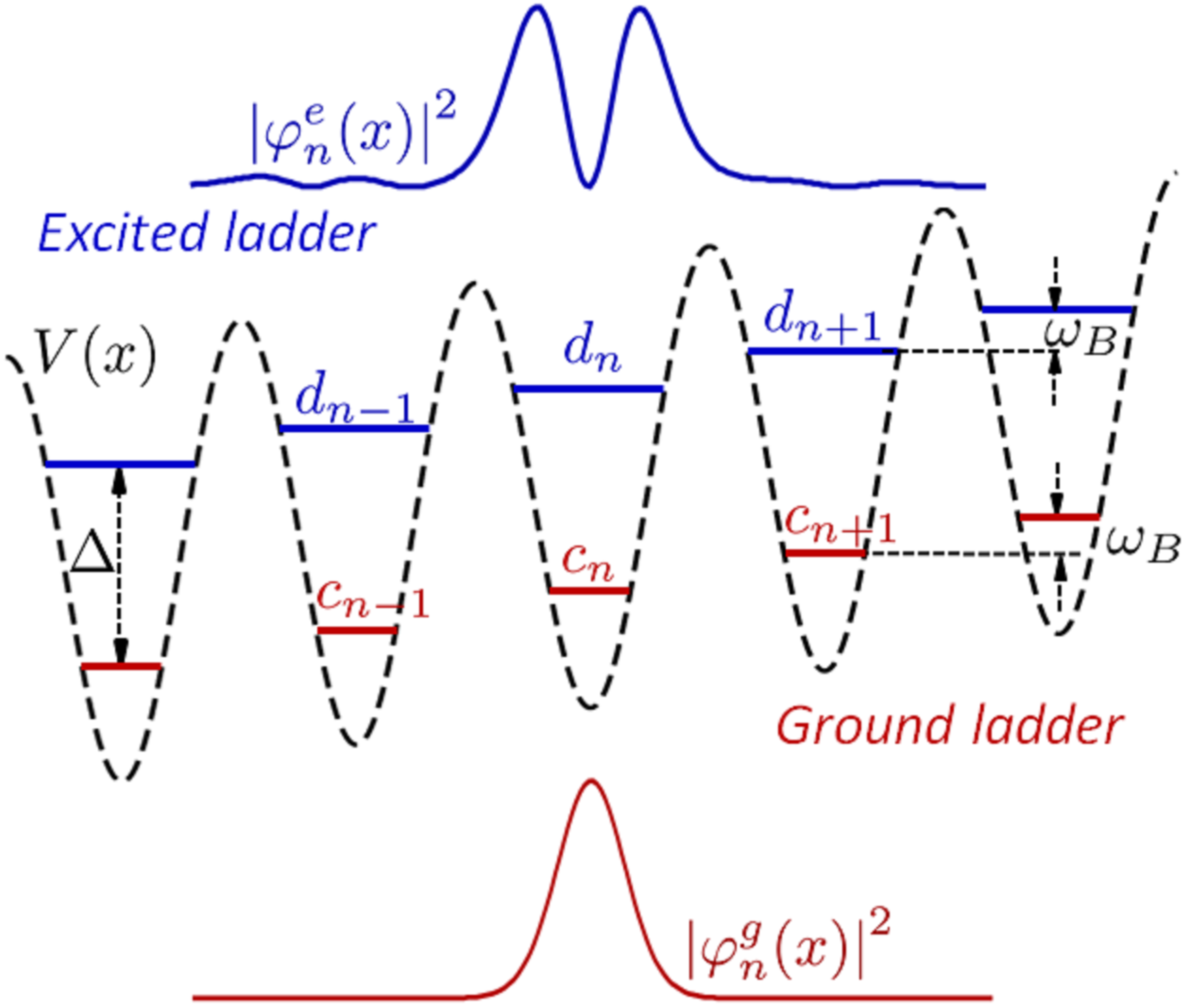
Figure 1: The Wannier-Stark system. Red energy levels $E_{n}^{g}$ and amplitude $c_{n}$ form the “ground” Wannier-Stark ladder, the corresponding spatial probability distribution $\left|\varphi_{n}^{g}(x)\right|^{2}$ (for site $n$) is shown as the bottom red curve. Blue levels of energy $E_{n}^{e}$ and amplitude $d_{n}$ form the “excited” WS ladder and the corresponding eigenstate $\left|\varphi_{n}^{e}(x)\right|^{2}$ is shown as the top blue curve. Levels in the same well are separated by an energy $\Delta$ and levels in the same ladder are separated by $\omega_{B}$, the Bloch frequency. The parameters used in this work are $V_{1}=6$, $F=1$, for which one finds numerically $\Delta=5.66$.

Compared to other works demonstrating ways to simulate Dirac physics, an advantage of our method is its simplicity both from the experimental and the theoretical point of view. We use simple 1D optical lattices modulated in time, for which analytic calculations can be pushed quite far. The system is realizable experimentally with state-of-the-art techniques (see Sec. VI). In particular, no Raman or Zeeman transitions are necessary. Moreover, the approach developed here is general and can be easily adapted to different situations, as it will be seen below (and in future works).

II The Dirac equation in a nutshell

The Dirac equation governs massive spin-1/2 particles (Dirac, 1928; Pal, 2011). As shown by Dirac, the requirement for relativistic invariance leads to the existence of spin and antiparticles; the theory deals with a spinor-4, that is, a 4-component state vector whose components are themselves wave functions:

$$\boldsymbol{\text{$\psi$}}=\left(\begin{array}[]{c}\psi_{1}(x,t)\\ \psi_{2}(x,t)\\ \psi_{3}(x,t)\\ \psi_{4}(x,t)\end{array}\right).$$

A possible representation for the Dirac equation for free particles of mass $m$ is $H\boldsymbol{\text{$\psi$}}=i\partial_{t}\boldsymbol{\text{$\psi$}}$, with the Dirac Hamiltonian

$$H=\left(\boldsymbol{\alpha}\cdot\boldsymbol{p}c+\beta mc^{2}\right)$$ (2)

where $\alpha_{j}$ ($j=x,y,z$) and $\beta$ are Dirac matrices

$$\alpha_{j}=\left(\begin{array}[]{cc}0&\sigma_{j}\\ \sigma_{j}&0\end{array}\right),\qquad\beta=\left(\begin{array}[]{cc}\mathbf{1}&0\\ 0&-\mathbf{1}\end{array}\right)$$

with $\sigma_{j}$ the Pauli matrices, $\mathbf{1}$ the $2\times 2$ identity matrix, $p_{j}=-i\partial/\partial x_{j}$ ($x_{j}=x,y,z$) the momentum operator, $c$ the velocity of light, and $\hbar=1$. For massive particles, in the rest frame of reference, the two upper components of the spinor-4 can be identified with the spin components of the (positive rest energy state) “particle” and the two bottom components with the spin of the “antiparticle” (negative rest energy state), but in a frame in which the particle is in motion, the components are mixed and no such distinction is possible; a spinor-4 description is necessary. However this “contamination” is small if $p\ll mc$. The general eigenvalues of the Dirac Hamiltonian are $\pm\left(p^{2}c^{2}+m^{2}c^{4}\right)^{1/2}$, the distinction between positive and negative eigenstates thus subsists (for a free particle) in all cases.

For a massive free particle, if the momentum is parallel to the spin, that is in the $z$ direction (the arbitrary quantization axis for the spin), then the Dirac equation couples $\psi_{1}$ to $\psi_{3}$ and $\psi_{2}$ to $\psi_{4}$. If the momentum is orthogonal to the spin (i.e. along the $x$- or the $y$-axis), it couples $\psi_{1}$ to $\psi_{4}$ and $\psi_{2}$ to $\psi_{3}$. Therefore, in both cases the quantum dynamics can be described by two spinor-2, obeying decoupled, equivalent equations. We can thus, for instance in the latter case, form the spinor-2

$$\bar{\boldsymbol{\psi}}=\left(\begin{array}[]{c}\psi_{2}\\ \psi_{3}\end{array}\right)$$

which, from Eq. (2), obeys the spinor-2 Dirac equation

$$i\partial_{t}\bar{\boldsymbol{\psi}}=c\sigma_{j}p_{j}\bar{\boldsymbol{\psi}}+mc^{2}\sigma_{z}\bar{\boldsymbol{\psi}}$$ (3)

where $j=x$ or $j=y$. A similar equation holds for $(\psi_{1},\psi_{4})$. In presence of a magnetic field, however, the quantization axis is imposed by the field and for an arbitrary direction of the momentum $\boldsymbol{p}$, the four components are coupled and the particle is described by a true spinor-4.

Equation (2) is the original Hamiltonian written by Dirac. This representation is well adapted to the case $p\ll mc$, where the first term is small compared to the second; if the first term is neglected, the Hamiltonian is diagonal. Other representations exist, e.g., the so-called Weyl representation corresponds to the Hamiltonian

$$H_{W}=c\left(\begin{array}[]{cc}\boldsymbol{\sigma}\cdot\boldsymbol{p}&0\\ 0&-\boldsymbol{\sigma}\cdot\boldsymbol{p}\end{array}\right)+\gamma_{0}mc^{2}.$$ (4)

with

$$\gamma_{0}=\left(\begin{array}[]{cc}0&\mathbf{1}\\ \mathbf{1}&0\end{array}\right).$$

This representation is well suited for the ultra-relativistic limit $p\gg mc$, where the mass term $\gamma_{0}mc^{2}$ in Eq. (4) becomes much smaller than the first one; neglecting the mass term leaves a diagonal form. For massless particles, the system separates into two subsets of equivalent equations, and can be described by a spinor-2, the so-called Weyl fermion. The above form implies that these particles are characterized by a well-defined projection of the spin along the particle’s momentum $\boldsymbol{\sigma}\cdot\boldsymbol{p}/|\boldsymbol{p}|$, a quantity called, as for photons, helicity.

III General model

In this section we introduce the general model leading from Wannier-Stark Hamiltonians of the form Eq. (1) to Dirac-like Hamiltonians. We shall consider a restricted state space of one or two ladders, i.e one or two WS states per potential well; the ground WS state (indexed by $\ell=g$) $\varphi_{n}^{g}(x)=\left\langle x\right.\left|\varphi_{n}^{g}\right\rangle$ in the well $n$, of energy $E_{n}^{g}=n\omega_{B}$, and the first excited WS state ($\ell=e$) $\varphi_{n}^{e}(x)$ of energy $E_{n}^{e}=E_{n}^{g}+\Delta$$=n\omega_{B}+\Delta$ of same well $n$ where $\varDelta$ is the energy offset between $g$ and $e$ levels in the same well (cf. Fig. 1). We assume in the following that none of these eigenenergies are degenerate.

The general evolution of an arbitrary wave function can then be written in the form

$$\Psi(x,t)= \sum_{n}\left[c_{n}(t)\exp\left(-iE_{n}^{g}t\right)\varphi_{n}^{g}(x)\right.$$

$$\left.+d_{n}(t)\exp\left(-iE_{n}^{e}t\right)\varphi_{n}^{e}(x)\right]$$ (5)

with $c_{n}(0)=\left\langle\varphi_{n}^{g}\right.\left|\Psi(0)\right\rangle$ and $d_{n}(0)=\left\langle\varphi_{n}^{e}\right.\left|\Psi(0)\right\rangle$.

We introduce a perturbation $\bar{H}(t)$ so that our complete Hamiltonian becomes $H=H_{0}+\bar{H}(t)$, with

$$\bar{H}(t)=-V_{1}\cos(2\pi x)f_{1}(t)+V_{2}\cos(\pi x)f_{2}(t)+V_{S}(x).$$ (6)

A suitable choice of the frequencies present in $f_{1}(t)$ and $f_{2}(t)$ induces interactions between states that are resonantly coupled, as shown in Fig. 2. For example, the ground-ladder level $\left|\varphi_{n}^{g}\right\rangle$ is resonantly coupled to excited-ladder level $\left|\varphi_{n+1}^{e}\right\rangle$ by a modulation of frequency $\Delta+\omega_{B}$, and to $\left|\varphi_{n-1}^{e}\right\rangle$ by a modulation of frequency $\Delta-\omega_{B}$, and so on. The perturbation term $V_{2}(x,t)=V_{2}\cos(\pi x)f_{2}(t)$ has double spatial period, and $V_{S}(x)$ is a static contribution whose utility will appear below.

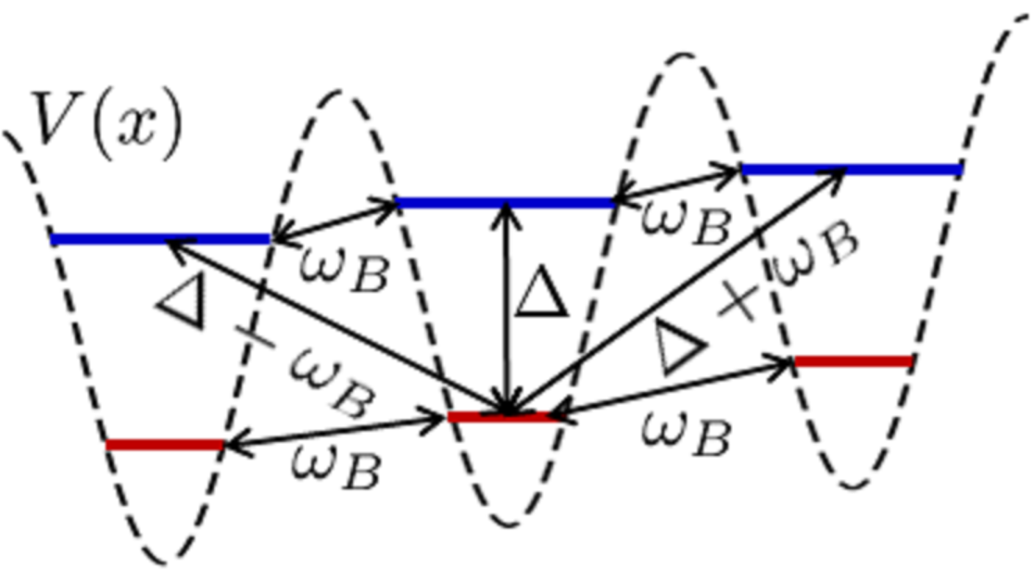
Figure 2: Energy levels and couplings in the Wannier-Stark system. A modulation of frequency $\omega_{B}$ induces an intra-ladder coupling between adjacent wells. Inter-ladder couplings are induced by perturbation frequencies $\Delta-\omega_{B}$ ($n\rightarrow n-1$), $\Delta$ ($n\rightarrow n$), and $\Delta+\omega_{B}$ ($n\rightarrow n+1$).

Under the action of $\bar{H}$ the coupled equations of motion for the amplitudes $c_{n}$ and $d_{n}$ of Eq. (5) are developed in App. A and have the form:

$$i\frac{d}{dt}c_{n}= \sum_{r\in\mathbb{Z}}\left\{\left\langle\varphi_{n}^{g}\right|\bar{H}\left|\varphi_{n+r}^{g}\right\rangle e^{-ir\omega_{B}t}c_{n+r}\right.$$

$$\left.+\left\langle\varphi_{n}^{g}\right|\bar{H}\left|\varphi_{n+r}^{e}\right\rangle e^{-ir\omega_{B}t}e^{-i\Delta t}d_{n+r}\right\}$$

$$i\frac{d}{dt}d_{n}= \sum_{r\in\mathbb{Z}}\left\{\left\langle\varphi_{n}^{e}\right|\bar{H}\left|\varphi_{n+r}^{g}\right\rangle e^{-ir\omega_{B}t}e^{i\Delta t}c_{n+r}\right.$$

$$\left.+\left\langle\varphi_{n}^{e}\right|\bar{H}\left|\varphi_{n+r}^{e}\right\rangle e^{-ir\omega_{B}t}d_{n+r}\right\}.$$ (7)

The functions $f_{\alpha}(t)$ ($\alpha=1,2$) appearing in $\bar{H}$, contain modulation frequencies of the form $\omega_{j,q}=j\omega_{B}+q\triangle$ with $j\in\mathbb{Z}$ and $q=0,\pm 1$

$$f_{\alpha}(t)=\sum_{j,q}\left(A_{j,q}^{(\alpha)}e^{ij\omega_{B}t}e^{iq\Delta t}\right)$$ (8)

where the reality condition implies $A_{j,q}^{(\alpha)}=A_{-j,-q}^{(\alpha)*}$. A great advantage of the Wannier-Stark model, within the assumption that parameters are such that there are no intrinsically degenerated states, is that tuning the amplitudes $A_{j,q}^{(\alpha)}$ allows us to choose which pairs of states are coupled, providing a very flexible control of the dynamics. For instance, one sees that modulations with $q=0$ induce intra-ladder couplings ($g-g$ and $e-e$) and modulations with $q=\pm 1$ induce inter-ladder couplings $e-g$; taking $j=0$ creates a coupling $g-e$ in the same well, whereas $j=1$ couples wells $n\rightarrow n+1$ and $j=-1$ couples $n\rightarrow n-1$.

In the resonant case, Eqs. (7) can be formally written as

$$i\frac{d}{dt}c_{n} =\sum_{r}\left(T_{n,r}^{gg}c_{n+r}+T_{n,r}^{ge}d_{n+r}\right)$$

$$i\frac{d}{dt}d_{n} =\sum_{r}\left(T_{n,r}^{ee}d_{n+r}+T_{n,r}^{eg}c_{n+r}\right)$$ (9)

(see App. A). The explicit form of coupling coefficients $T_{n,r}^{ab}$ ($a,b\in\left\{e,g\right\}$) between the sites $n$ and $n+r$ depend on the overlap integrals, which, thanks to the properties of the WS states, are

$$\left\langle\varphi_{n}^{g,e}\right|\cos(2\pi x)\left|\varphi_{n+r}^{g,e}\right\rangle=\left\langle\varphi_{0}^{g,e}\right|\cos(2\pi x)\left|\varphi_{r}^{g,e}\right\rangle,$$

$$\left\langle\varphi_{n}^{g,e}\right|\cos(\pi x)\left|\varphi_{n+r}^{g,e}\right\rangle=(-1)^{n}\left\langle\varphi_{0}^{g,e}\right|\cos(\pi x)\left|\varphi_{r}^{g,e}\right\rangle.$$

One then obtains intra-ladder coupling as

$$T_{n,r}^{gg}=\left\langle\varphi_{n}^{g}\right|V_{S}\left|\varphi_{n}^{g}\right\rangle\delta_{r,0}- V_{1}A_{r,0}^{(1)}\left\langle\varphi_{0}^{g}\right|\cos(2\pi x)\left|\varphi_{r}^{g}\right\rangle$$

$$+(-1)^{n}V_{2}A_{r,0}^{(2)}\left\langle\varphi_{0}^{g}\right|\cos(\pi x)\left|\varphi_{r}^{g}\right\rangle$$

$$T_{n,r}^{ee}=\left\langle\varphi_{n}^{e}\right|V_{S}\left|\varphi_{n}^{e}\right\rangle\delta_{r,0}- V_{1}A_{r,0}^{(1)}\left\langle\varphi_{0}^{e}\right|\cos(2\pi x)\left|\varphi_{r}^{e}\right\rangle$$

$$+(-1)^{n}V_{2}A_{r,0}^{(2)}\left\langle\varphi_{0}^{e}\right|\cos(\pi x)\left|\varphi_{r}^{e}\right\rangle.$$ (10)

and inter-ladder couplings

$$T_{n,r}^{ge}= -V_{1}A_{r,1}^{(1)}\left\langle\varphi_{0}^{g}\right|\cos(2\pi x)\left|\varphi_{r}^{e}\right\rangle$$

$$+(-1)^{n}V_{2}A_{r,1}^{(2)}\left\langle\varphi_{0}^{g}\right|\cos(\pi x)\left|\varphi_{r}^{e}\right\rangle$$

$$T_{n,r}^{eg}= -V_{1}A_{r,-1}^{(1)}\left\langle\varphi_{0}^{e}\right|\cos(2\pi x)\left|\varphi_{r}^{g}\right\rangle$$

$$+(-1)^{n}V_{2}A_{r,-1}^{(2)}\left\langle\varphi_{0}^{e}\right|\cos(\pi x)\left|\varphi_{r}^{g}\right\rangle.$$ (11)

This general model spans all cases we will consider in the present work. In Sec. IV we show how to construct a quantum simulator for a spinor-2 Dirac equation, and in Sec. V we show how the full spinor-4 Dirac or Weyl equations can be synthesized.

IV Spinor-2 model

Many interesting phenomena related to the Dirac equation can be illustrated with a simpler spinor-2. In order to construct a spinor-2 quantum simulator we restrict our system to the ground state ladder with “self” ($c_{n}$$\leftrightarrows c_{n}$) and nearest neighbors ($c_{n}\leftrightarrows c_{n\pm 1}$) couplings. Inter-ladder transitions are set off by keeping only the $q=0$ term in Eq. (8), and we start with an initial condition $d_{n}(0)=0$ for all sites , so that the excited ladder is never populated. We also set $V_{1}=V_{S}=0$ in Eq. (6). The perturbation thus contains only contributions of double spatial period

$$\bar{H}=V_{2}f_{2}(t)\cos(\pi x)$$ (12)

with, in Eq. (8), $j=0,\pm 1$, $q=0$, that is

$$f_{2} (t)=A_{0,0}^{(2)}+A_{1,0}^{(2)}e^{i\omega_{B}t}+A_{-1,0}^{(2)}e^{-i\omega_{B}t}$$

$$=A_{0}+A_{1}e^{i\omega_{B}t}+A_{1}^{*}e^{-i\omega_{B}t},$$ (13)

where, in the second line, we suppressed for simplicity the fixed indexes $q=0$ and $\alpha=2$. The remaining coupling parameters are then [Eq. (10)]

$$T_{n,1}^{gg} =(-1)^{n}V_{2}A_{1}\left\langle\varphi_{0}^{g}\right|\cos(\pi x)\left|\varphi_{1}^{g}\right\rangle$$

$$T_{n,0}^{gg} =(-1)^{n}V_{2}A_{0}\left\langle\varphi_{0}^{g}\right|\cos(\pi x)\left|\varphi_{0}^{g}\right\rangle$$

$$T_{n,-1}^{gg} =(-1)^{n}V_{2}A_{-1}\left\langle\varphi_{0}^{g}\right|\cos(\pi x)\left|\varphi_{-1}^{g}\right\rangle$$

$$=-(-1)^{n}V_{2}A_{1}^{*}\left\langle\varphi_{0}^{g}\right|\cos(\pi x)\left|\varphi_{1}^{g}\right\rangle.$$

Eqs. (9) then imply

$$i\frac{d}{dt}c_{n}= (-1)^{n}V_{2}A_{0}\left\langle\varphi_{0}^{g}\right|\cos(\pi x)\left|\varphi_{0}^{g}\right\rangle c_{n}$$

$$(-1)^{n}V_{2}\left\langle\varphi_{0}^{g}\right|\cos(\pi x)\left|\varphi_{1}^{g}\right\rangle\left[A_{1}c_{n+1}-A_{1}^{*}c_{n-1}\right].$$ (14)

A key point for realizing a spinor-2 system is that the perturbation of double spatial period creates alternate sign couplings from site to site (see App. A). This has a dynamical effect that is clearly visible in the reciprocal space, where we define “spin” states as “odd site” and “even site” amplitudes

$$\bar{c}_{+}(k,t) = \sum_{n}e^{2ink}c_{2n}(t)$$

$$\bar{c}_{-}(k,t) = \sum_{n}e^{i(2n+1)k}c_{2n+1}(t).$$ (15)

Taking, for simplicity, $A_{1}$ real in Eq. (14), one obtains the following coupled set of equations

$$i\frac{d}{dt}\bar{c}_{+}(k,t) = E_{0}\bar{c}_{+}(k,t)-2i\Omega_{2}\sin k\>\bar{c}_{-}(k,t)$$

$$i\frac{d}{dt}\bar{c}_{-}(k,t) = -E_{0}\bar{c}_{-}(k,t)+2i\Omega_{2}\sin k\>\bar{c}_{+}(k,t),$$ (16)

where we defined the frequency $\Omega_{2}=$$V_{2}A_{1}\left\langle\varphi_{0}^{g}\right|\cos(\pi x)\left|\varphi_{1}^{g}\right\rangle$ and the “self-energy” $E_{0}=$$V_{2}A_{0}\left\langle\varphi_{0}^{g}\right|\cos(\pi x)\left|\varphi_{0}^{g}\right\rangle$. These two equations show the emergence of an effective pseudo spinor-2 which in $k$-space is

$$\bar{\boldsymbol{\psi}}=\left(\begin{array}[]{c}c_{+}(k,t)\\ c_{-}(k,t)\end{array}\right).$$

Looking for solutions in $\exp\left(-i\omega(k)t\right)$, the corresponding eigenenergies $\omega(k)$ are

$$\omega_{\pm}(k)=\pm\sqrt{E_{0}^{2}+4\Omega_{2}^{2}\sin^{2}k}.$$ (17)

For $E_{0}=0$, the positive and negative eigenenergies $\pm 2\left|\Omega_{2}\sin k\right|$ are associated to the eigenspinor

$$\bar{\boldsymbol{\psi}}_{\pm}=\frac{1}{\sqrt{2}}\left(\begin{array}[]{c}1\\ \pm i\mathrm{sgn}(\Omega_{2}k)\end{array}\right),$$ (18)

where $\mathrm{sgn}(x)$ is the sign function. The linear, phonon-like, dispersion relation for $k\rightarrow 0$ , $\omega_{\pm}(k)=\pm 2\left|\Omega_{2}k\right|$, reproduces the spectrum of the relativistic massless spin-1/2 fermion. A “1D-conical intersection” occurs as the two branches coalesce at $k=0$, creating a so-called Dirac point.

In real space, if the even- $c_{2n}(x,t)$ and odd-site $c_{2n+1}(x,t)$ amplitudes vary slowly on the scale of the lattice step $a=1$, one can take the continuous limit of Eqs. (14), and define the functions $c_{\pm}(x,t)$ as the spatial envelopes of the $c_{n}(x,t)$ (cf. App. A), leading to the spinor-2

$$\boldsymbol{\phi}=\left(\begin{array}[]{c}c_{+}(x,t)\\ c_{-}(x,t)\end{array}\right)$$

which obeys an equation

$$i\partial_{t}\boldsymbol{\phi}=-2\Omega_{2}(-i\partial_{x})\sigma_{y}\boldsymbol{\phi}+E_{0}\sigma_{z}\boldsymbol{\phi}$$ (19)

of the same form as Eq. (3) if one sets $p_{y}=-i\partial_{x}$ (the labeling of the axes is obviously arbitrary). By comparing Eqs. (19) and (2) we can make the following identifications: $E_{0}=\overline{m}\overline{c}^{2}$ and $2\left|\Omega_{2}\right|=\overline{c}$, where $\overline{m}$ and $\overline{c}$ are the effective mass and speed of light which can be adjusted by changing the modulation amplitudes $A_{0}$ and $A_{1}$ in Eq. (13).

The validity of the model Eq. (16) can be numerically tested by comparison with the simulation of the exact Schrödinger equation corresponding to the Hamiltonian $H_{0}+\bar{H}$ with $\bar{H}$ given by Eq. (12). We chose a broad initial wave packet, with amplitudes:

$$c_{2n} =a_{+}G^{(k_{0})}(2n),\;c_{2n+1}$$ (20)

$$=a_{-}G^{(k_{0})}(2n+1),$$ (21)

with $G^{(k_{0})}(n)=\left(2\pi/\sigma\right)^{1/2}$$\exp\left(-ink_{0}\right)$$\exp\left(-n^{2}/\sigma^{2}\right)$, $\sigma\gg 1,$ with the normalization condition $\left|a_{+}\right|^{2}+\left|a_{-}\right|^{2}=1$. The initial spinor is thus

$$\boldsymbol{\phi}_{0}=\left(\begin{array}[]{c}a_{\text{+}}\\ a_{-}\end{array}\right)G^{(k_{0})}(x)\leftrightarrow\left(\begin{array}[]{c}a_{\text{+}}\\ a_{-}\end{array}\right)\bar{G}^{(k_{0})}(k)$$ (22)

where the first expression is in real and the second in momentum space, and $\bar{G}^{(k_{0})}(k)$ is a narrow Gaussian function centered at $k=k_{0}$.

The dashed lines in Fig. 3 show the dynamical behavior of a massless particle (setting $A_{0}=0$ in Eq. (13) leads to $E_{0}=0$) obtained from the above model [cf. Eq. (14)] at time $t=0,$ $150T_{B}$ and $300T_{B}$, where $T_{B}=2\pi/F$ is the Bloch-period. The initial spinor $(a_{+},a_{-})=(1,0)$ with $k_{0}\rightarrow 0^{+}$, corresponds to a superposition of the positive energy eigenspinor $(1,i)/\sqrt{2}$ and the negative energy eigenspinor $(1,-i)/\sqrt{2}$ [cf. Eq. (18)] having opposite drift velocities $\pm v_{D}$ which from Eq. (17) read

$$v_{D}=\left|\frac{d\omega_{\pm}}{dk}\right|_{k_{0}}=2\left|\Omega_{2}\cos k_{0}\right|\simeq 2\left|\Omega_{2}\right|.$$

The comparison with the solution of exact Schrödinger equation (full lines) shows a very good agreement up to $t=300T_{B}$. One can verify that splitting into two separate wave packets moving with opposite group velocities $\pm v_{D}$ which matches the expected theoretical value.

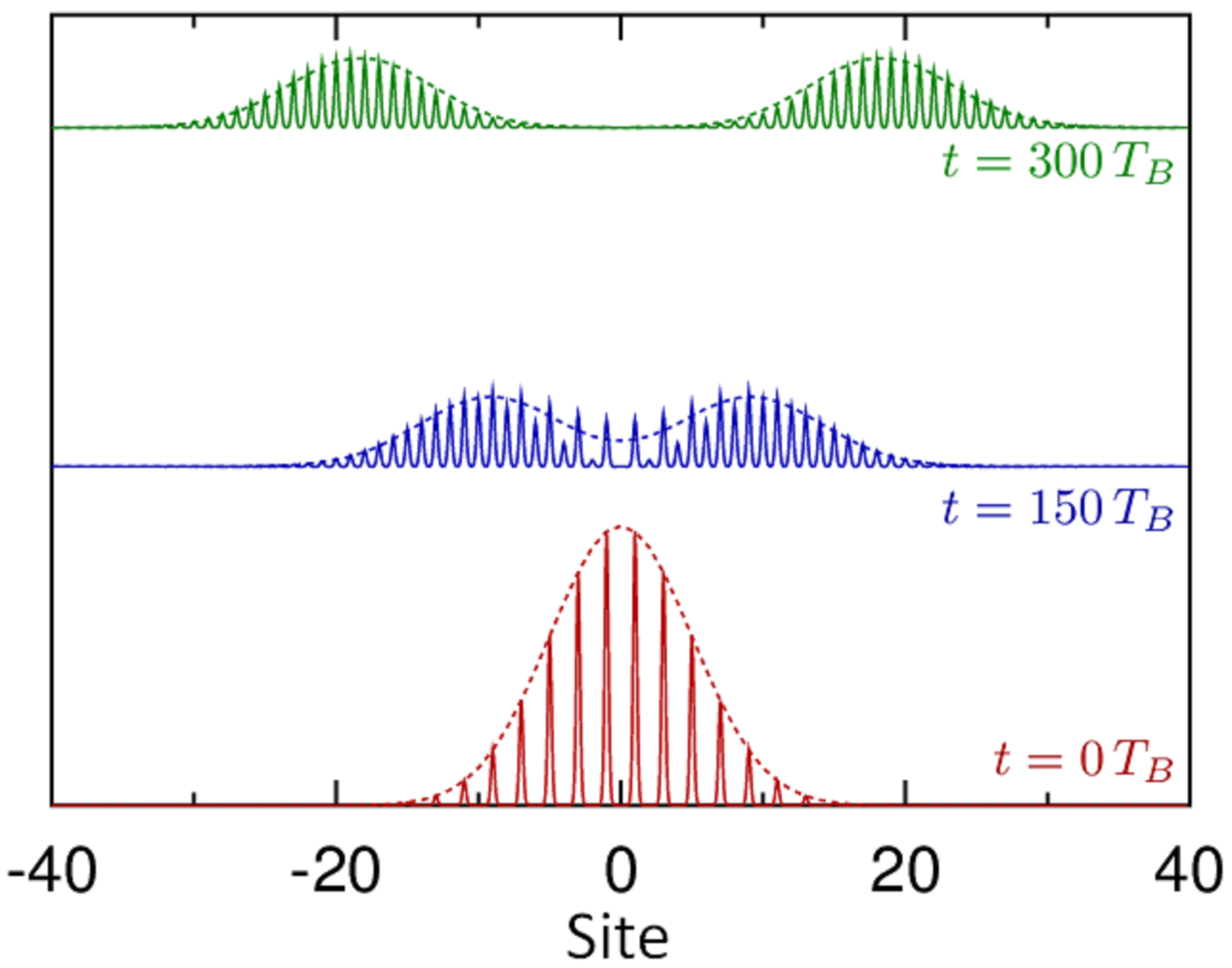
Figure 3: Evolution of an initial wave packet with $k_{0}=0$, $\sigma=10$ and $(a_{+},a_{-})=(1,0)$ [Eq. (20)] using the discrete model given by Eq. (14) (dashed lines), at times $t=0$ (red bottom line), $150T_{B}$ (blue middle line) and $300T_{B}$ (top green line) and compared to the exact Schrödinger equation simulation (full lines). Parameters are $V_{1}=6$, $F=1,$ $\bar{H}(x,t)=0.5\cos\left(\pi x\right)\cos\left(\omega_{B}t\right)$ which give $\left\langle\varphi_{0}^{g}\right|\cos(\pi x)\left|\varphi_{1}^{g}\right\rangle=-2.31\times 10^{-2}$ (numerical value), and $\Omega_{2}=-5.4\times 10^{-3}$. The numerical value of the drift velocity $v_{D}$ agrees with the theoretical value $v_{D}=2\left|\Omega_{2}\cos k_{0}\right|=1.1\times 10^{-2}$.

One of the most characteristic effects associated to the Dirac equation for massive particles is the so-called Zitterbewegung (“trembling motion”), an interference effect between the positive and negative energy parts of the spinor resulting in a spatial jitter of the wave packet Vaishnav and Clark (2008). Such an effect was recently observed in quantum simulators of the Dirac equation with trapped ions (Gerritsma et al., 2010), with ultracold atoms LeBlanc et al. (2013); Qu et al. (2013), and in a photonic device Dreisow et al. (2010); Longhi (2010). Figure 4 shows the spatio-temporal behavior of a wave packet for a massive particle governed by Eqs. (14), with a an initial spinor $(a_{+},a_{-})=2^{-1/2}(1,1)$ and $k_{0}=0$, corresponding to superposition of positive and negative energy eigenstates (as can be seen from Eq. (16) in the limit $k\rightarrow 0$). In order to give a mass to the particle, we set $A_{0}\neq 0$ in Eq. (13), so that $E_{0}\neq 0$). We verified that the same spatio-temporal behavior is obtained from the exact Schrödinger equation.

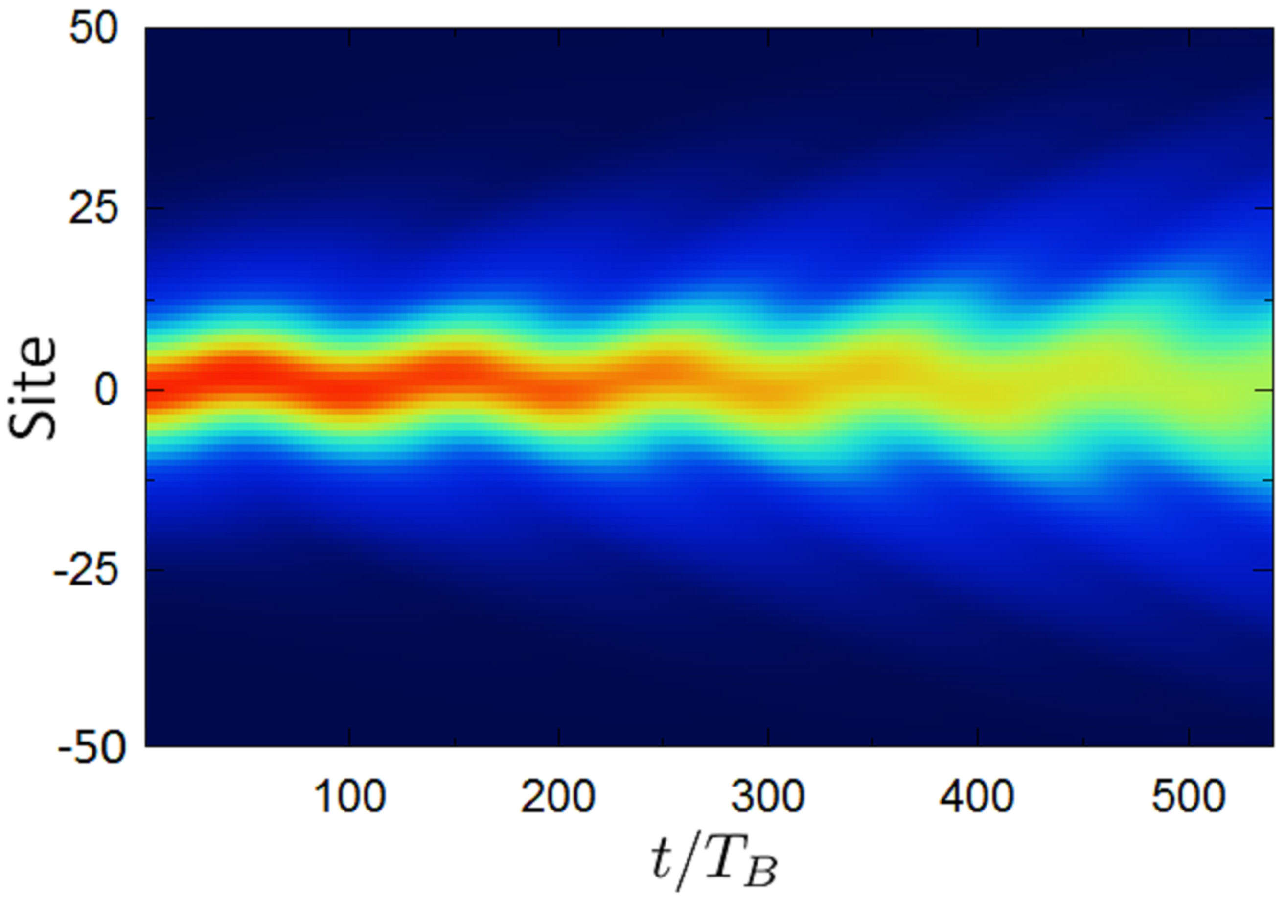
Figure 4: Zitterbewegung obtained from the discrete model Eq. (14) with initial spinor $(a_{+},a_{-})=2^{-1/2}(1,1)$, $\sigma=10$ and $k_{0}=0$. The probability density is displayed in false colors. Potential parameters are the same as in Fig. 3 except $\bar{H}(x,t)=\cos\pi x\left(0.5\cos\omega_{B}t+0.005\right)$. The time-independent contribution $A_{0}=0.005$ in $\bar{H}$ leads to a mass term $E_{0}=4.6\times 10^{-3}$.

From Eq. (16) one can obtain the evolution of the wave packet’s average position

$$\frac{d\left\langle x\right\rangle}{dt} =\frac{1}{i\hbar}\left\langle\left[x,H\right]\right\rangle=-2\Omega_{2}\left\langle\sigma_{y}\right\rangle$$

$$=2i\Omega_{2}\int dx\left(c_{+}^{*}(x,t)c_{-}(x,t)-\mathrm{c.c.}\right)$$

$$=2i\Omega_{2}\int dk\left(\bar{c}_{+}^{*}(k,t)\bar{c}_{-}(k,t)-\mathrm{c.c.}\right).$$

The fact that the oscillation depends on $c_{+}^{*}c_{-}$ (in real or momentum space) shows that the Zitterbewegung is due to the coherence between positive- and negative-energy states, confirming its physical interpretation as a quantum beat between odd- and even- site contributions (or positive and negative energy states in Dirac’s language). To the leading order in $k\approx 0$ we find

$$\frac{d\left\langle x\right\rangle}{dt}=\frac{i2\Omega_{2}}{\sqrt{1-iDt}}a_{+}^{*}a_{-}e^{2iE_{0}t}+\mathrm{c.c}$$ (23)

with $D=4\Omega_{2}^{2}/(E_{0}\sigma^{2})$. In this approximation, the amplitude of the oscillation is seen to be directly proportional to the initial coherence $a_{+}^{*}a_{-}$. The oscillation has frequency $2E_{0}$, as it is the case for the electron’s Zitterbewegung, and is slowly damped by diffusion effects with an effective coefficient $D$; note that the amplitude of the oscillation for $Dt\rightarrow 0$, is $\left|\Omega_{2}\right|/E_{0}=(2\bar{m}\overline{c})^{-1}$, that is, half the dimensionless Compton wavelength, also in agreement with the Zitterbewegung of an electron. As shown in Fig. 5, the numerical calculations of $\left\langle x(t)\right\rangle$ from the exact Schrödinger equation and from the discrete model are in excellent agreement and match the theoretical amplitude and period deduced from Eq. (23).

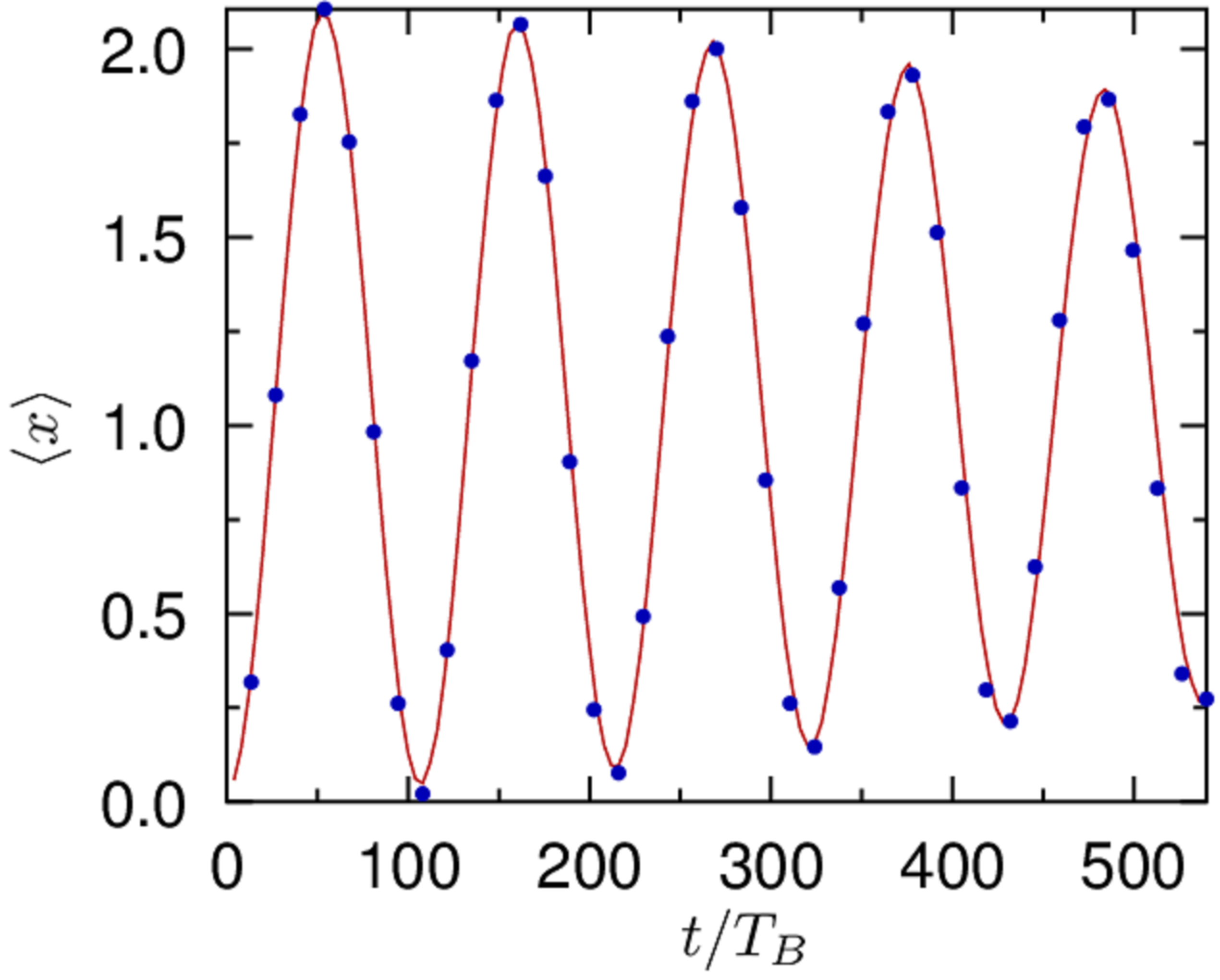
Figure 5: Evolution of the average position $\left\langle x(t)\right\rangle$ for $0\leq t\leq 5T_{ZB}$. Solid red line: Numerical result obtained from the exact Schrödinger equation. Blue circles: calculation from the discrete model Eq. (14). Same parameters as in Fig. 4. The Zitterbewegung period is in excellent agreement with the theoretical value, $T_{ZB}=2\pi/(2E_{0})=109T_{B}$, and its amplitude with the prediction $\left|\Omega_{2}\right|/E_{0}=1.17$. Due to diffusion, the amplitude is attenuated by a factor $(1+D^{2}t^{2})^{-1/2}\sim 0.75$ at $t=5T_{ZB}$ as compared to its initial value.

The effective parameters $\overline{m}=E_{0}/4\Omega_{2}^{2}$ and $\overline{c}=2\left|\Omega_{2}\right|$ can be calculated from the parameters used in the above simulations. For atoms of mass $M$, they read, in dimensioned units, $\overline{\mathsf{c}}=2\left|\Omega_{2}\right|E_{R}d/\hbar$$=\left|\Omega_{2}\right|\left(2\pi^{2}\hbar/M\lambda_{L}\right)$ and $\overline{\mathsf{m}}=E_{0}E_{R}/c^{2}$$=\left(E_{0}/2\pi^{2}\Omega_{2}^{2}\right)M$. For cesium atoms and for potential parameters chosen in this section ($E_{0}=4.6\times 10^{-3}$, $\left|\Omega_{2}\right|=5.4\times 10^{-3}$) this leads to $\overline{\mathsf{m}}\sim 9.3M$ and $\overline{\mathsf{c}}\sim 1.33\times 10^{-4}\left|\Omega_{2}\right|$$\sim 7\times 10^{-7}$m/s$\approx 2\times 10^{-3}v_{R}$, where $v_{R}=\sqrt{2E_{R}/M}$ is the atom recoil velocity .

V Spinor-4 model

We can also construct a full Dirac equation with a spinor-4. Using different coupling schemes we obtain either a Dirac-like equation in the standard representation or its analog in the Weyl representation. This beautifully illustrates the flexibility of the general model presented in Sec. III.

V.1 Spinor-4 Dirac representation

In order to construct a spinor-4 in the Dirac representation, we consider both ground and excited WS ladders, nearest-neighbors inter-ladder couplings are set on and intra-ladder couplings are set off. The perturbation is thus of the form [cf. Eq. (6)]

$$\bar{H}=-V_{1}f_{1}(t)\cos(2\pi x)+V_{S}(x)$$

with the modulation function

$$f_{1}(t)=A_{1,1}^{(1)}e^{i\omega_{B}t}e^{i\Delta t}+A_{1,-1}^{(1)}e^{i\omega_{B}t}e^{-i\Delta t}+\mathrm{c.c}.$$

From Eq. (9) we obtain the equations of motion

$$i\frac{d}{dt}c_{n} = T_{n,0}^{gg}c_{n}+T_{n,1}^{ge}d_{n+1}+T_{n,-1}^{ge}d_{n-1}$$

$$i\frac{d}{dt}d_{n} = T_{n,0}^{ee}d_{n}+T_{n,1}^{eg}c_{n+1}+T_{n,-1}^{eg}c_{n-1}$$

with

$$T_{n,-1}^{eg}=\left(T_{n,1}^{ge}\right)^{*},\;T_{n,1}^{eg}=\left(T_{n,-1}^{g,e}\right)^{*}.$$

A Dirac-like equation is obtained if the coupling coefficients $T_{n,1}^{ge}=-T_{n,-1}^{ge}$ are imaginary and if $A_{1,1}^{(1)}\left\langle\varphi_{0}^{g}\right|\cos(2\pi x)\left|\varphi_{1}^{e}\right\rangle$$=-A_{1,-1}^{(1)}\left\langle\varphi_{1}^{g}\right|\cos(2\pi x)\left|\varphi_{0}^{e}\right\rangle$, a condition that is realized by tuning the modulation amplitudes $A_{1,\pm 1}^{(1)}$ so that they exactly compensate for the difference in the overlap integrals. The static perturbation $V_{S}(x)$ is chosen to be translation-invariant with respect to the reference lattice constant $a=1$, so that $T_{n,0}^{gg}=\left\langle\varphi_{0}^{g}\right|V_{S}\left|\varphi_{0}^{g}\right\rangle\equiv V_{S}^{g}$ and $T_{n,0}^{ee}=\left\langle\varphi_{0}^{e}\right|V_{S}\left|\varphi_{0}^{e}\right\rangle\equiv V_{S}^{e}$ do not depend on $n$; the simple form used here is $V_{S}(x)\propto\cos\left(4\pi x\right)$. Thus

$$i\frac{d}{dt}c_{n} = E_{0}c_{n}+i\Omega_{1}\left(d_{n+1}-d_{n-1}\right)$$

$$i\frac{d}{dt}d_{n} = -E_{0}d_{n}+i\Omega_{1}\left(c_{n+1}-c_{n-1}\right)$$ (24)

where the coupling $\Omega_{1}$ is given by

$$i\Omega_{1}=T_{n,1}^{ge}=-V_{1}A_{1,1}^{(1)}\left\langle\varphi_{0}^{g}\right|\cos(2\pi x)\left|\varphi_{1}^{e}\right\rangle$$

(with $A_{1,1}^{(1)}$ imaginary) and the effective rest mass $E_{0}$, controlled by the static potential $V_{S}(x),$ is given by 

$$E_{0} =\frac{V_{S}^{g}-V_{S}^{e}}{2}.$$ (25)

The coupled equations (24) can be split into two independent sub-lattices corresponding to sites $c_{n}$ with $n$ even coupled to $d_{n}$ with $n$ odd and conversely. Hence, we can build a 4-component Wannier-Stark spinor

$$\boldsymbol{\psi}=\left(\begin{array}[]{c}c_{+}\\ c_{-}\\ d_{+}\\ d_{-}\end{array}\right)$$ (26)

where $c_{\pm}(x,t)$ and $d_{\pm}(x,t)$ are the slowly varying envelopes of $c_{n}$ and $d_{n}$ for $n$ odd and $n$ even respectively (in close analogy with what has been done in the spinor-2 case, Sec. IV and in App. A), giving

$$i\partial_{t}\boldsymbol{\psi}=\left(E_{0}\beta-2\Omega_{1}\alpha_{x}p_{x}\right)\boldsymbol{\psi}$$ (27)

which corresponds to the Dirac equation described by Eq. (2). As stated in Sec. II, this equation can be decoupled into two equivalent sets

$$i\frac{\partial}{\partial t}\left(\begin{array}[]{c}c_{+}\\ d_{-}\end{array}\right)=\left(E_{0}\sigma_{z}-2\Omega_{1}p_{x}\sigma_{x}\right)\left(\begin{array}[]{c}c_{+}\\ d_{-}\end{array}\right)$$

the other components $(c_{-},d_{+})$ following exactly the same equation. The corresponding dispersion relation is again $\omega_{\pm}(k)=\pm\left(E_{0}^{2}+4\Omega_{1}^{2}k^{2}\right)^{1/2}$, but each eigenvalue has now a double degeneracy. Note that this degeneracy can be lifted by adding other terms in $\bar{H}$ (for instance, terms proportional to $\cos(\pi x)$ which break translation invariance with respect to the lattice step $a=1$) and will be studied in a forthcoming paper.

The Zitterbewegung is described in the same way as for the spinor-2 case:

$$\frac{d\left\langle x\right\rangle}{dt}= -2\Omega_{1}\left\langle\alpha_{x}\right\rangle$$

$$= -2\Omega_{1}\intop dx\left[c_{+}^{*}(x,t)d_{-}(x,t)+\mathrm{c.c}\right.$$

$$+\left.c_{-}^{*}(x,t)d(x,t)+\mathrm{c.c.}\right].$$

In the simple case $p_{x}=0$ with a spatially broad initial wave packet $\boldsymbol{\psi}=$$2^{-1}(a_{+},a_{-},b_{+},b-)G^{(k_{0})}(x)$ one obtains

$$\frac{d\left\langle x\right\rangle}{dt}=-2\Omega_{1}\left[\left(a_{+}^{*}b_{-}+a_{-}^{*}b_{+}\right)\,e^{2iE_{0}t}+\mathrm{c.c.}\right]$$

showing an oscillation amplitude proportional to $\Omega_{1}/E_{0}$, controlled by the initial coherence. The superposition of a “spin up particle” $(a_{\text{+}},a_{-})$ and a “spin down antiparticle” $(b_{\text{+}},b_{-})$ $\boldsymbol{\psi}=2^{-1}(1,1,1,1)$ , leads to $\left\langle x(t)\right\rangle=-\left(\Omega_{1}/E_{0}\right)\sin(2E_{0}t)$. States with $\left(a_{+}^{*}b_{-}+a_{-}^{*}b_{+}\right)=0$, for instance $\boldsymbol{\psi}=2^{-1}(1,-1,1,1)$, display no Zitterbewegung. These results are illustrated in Fig. 6. The oscillations (blue line) obtained from the Schrödinger equation are in good agreement with the simulation of Eq. (24) displayed in red. On the time scale of a few Zitterbewegung periods $T_{ZB}=1/2E_{0}$, diffusion effects are here negligible (one finds $DT_{ZB}=4\Omega_{1}^{2}\pi/(E_{0}^{2}\sigma^{2})\sim 10^{-2}$), but in contrast to the spinor-2 model displayed in Fig. 5, the exact Schrödinger equation shows parasitic Landau-Zener tunneling into the continuum (due to the presence of populated excited states $d_{\pm}$), leading to a slow decrease in the spinor negative-energy amplitudes and thus to the oscillation amplitude. Fast, small-amplitude Rabi oscillations at frequency $\Omega_{1}\gg T_{ZB}^{-1}$ between ground and excited states are responsible for the apparent thickening of the blue line in Fig. 6: it is due to the asymmetry of the excited state $\varphi_{n}^{e}(x)$ with respect to the center of its well $n$ leading thus an average position which differs by a fraction of a lattice step as compared to the ground state average position. Note finally that the second initial condition spinor $\boldsymbol{\psi}=2^{-1}(1,-1,1,1)$ (green line) do not display Zitterbewegung, as expected.

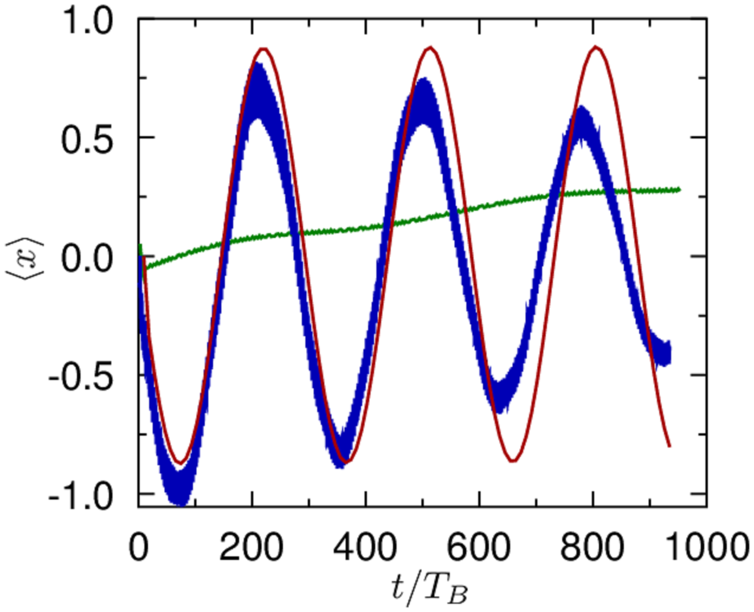
Figure 6: Evolution of the average position $\left\langle x(t)\right\rangle$ for $0\leq t\leq 3T_{ZB}$. Exact Schrödinger equation (thick blue line) and discrete model Eq. (24) (red line) for an initial spinor $2^{-1}(1,1,1,1)$, $\sigma^{2}=500$ and $k_{0}=0$. The non-oscillating green line is the exact Schrödinger equation result for an initial spinor $2^{-1}(1,-1,1,1)$, which does not show Zitterbewegung. Potential parameters are $V_{1}=6$, $F=1$, $A_{1,1}^{(1)}=-5.0\times 10^{-3}i$ and $A_{1,-1}^{(1)}=-7.5\times 10^{-3}i$ giving $\Omega_{1}=-1.5\times 10^{-3}$. The effective mass $E_{0}=1.6\times 10^{-3}$ is generated by the potential $V_{S}(x)=5\times 10^{-3}\cos(4\pi x)$. The Zitterbewegung period and amplitude agree with the theoretical values $T_{ZB}=2\pi/(2E_{0})=310T_{B}$ and $\left|\Omega_{1}\right|/E_{0}=0.93$.

V.2 Spinor-4 Weyl representation

A Dirac equation in the Weyl representation can be obtained with a different coupling scheme. The calculation follows the same lines as in the previous section, and we shall simply indicate the main steps below. We use the Hamiltonian $\bar{H}$ of Eq. (6) with $V_{S}(x)=0$ and with the modulations

$$f_{2}(t) =A_{1,1}^{(2)}e^{i\omega_{B}t}e^{i\Delta t}+A_{1,-1}^{(2)}e^{i\omega_{B}t}e^{-i\Delta t}+\mathrm{c.c.}$$

$$f_{1}(t) =A_{0,1}^{(1)}e^{i\Delta t}+\mathrm{c.c}.$$

The general developments of Sec. III then lead to:

$$i\frac{d}{dt}c_{n} =T_{n,1}^{ge}d_{n+1}+T_{n,-1}^{ge}d_{n-1}+T_{n,0}^{ge}d_{n}$$

$$i\frac{d}{dt}d_{n} =T_{n,1}^{eg}c_{n+1}+T_{n,-1}^{eg}c_{n-1}+T_{n,0}^{eg}c_{n}.$$

We then choose $A_{0,1}^{(1)}$ real and define the real parameter

$$E_{W} =T_{n,0}^{ge}=T_{n,0}^{eg}$$

$$=-A_{0,1}^{(1)}V_{1}\left\langle\varphi_{0}^{g}\left|\cos(2\pi x)\right|\varphi_{0}^{e}\right\rangle.$$

Making the amplitudes $A_{1,\pm 1}^{(2)}$ imaginary and tuning them in such a way that $A_{1,1}^{(2)}\left\langle\varphi_{0}^{g}\right|\cos(\pi x)\left|\varphi_{1}^{e}\right\rangle$$=A_{-1,1}^{(2)}\left\langle\varphi_{1}^{g}\right|\cos(\pi x)\left|\varphi_{0}^{e}\right\rangle$, one has

$$T_{n,1}^{ge} =(-1)^{n}V_{2}A_{1,1}^{(2)}\left\langle\varphi_{0}^{g}\right|\cos(\pi x)\left|\varphi_{1}^{e}\right\rangle=i(-1)^{n}\Omega_{W}$$

$$T_{n,-1}^{ge} =(-1)^{n}V_{2}A_{-1,1}^{(2)}\left\langle\varphi_{0}^{g}\right|\cos(\pi x)\left|\varphi_{-1}^{e}\right\rangle=-i(-1)^{n}\Omega_{W}$$

$$T_{n,1}^{eg} =T_{n,1}^{ge}$$

$$T_{n,-1}^{eg} =-T_{n,1}^{ge}$$

and thus

$$i\frac{d}{dt}c_{n}= (-1)^{n} i\Omega_{W}\left(d_{n+1}-d_{n-1}\right)+E_{W}d_{n}$$

$$i\frac{d}{dt}d_{n}= -(-1)^{n} i\Omega_{W}\left(c_{n+1}-c_{n-1}\right)+E_{W}c_{n}.$$ (28)

The continuous limit of these two equations gives

$$i\partial_{t}c_{+}(x,t) =-2\Omega_{W}p_{x}d_{-}+E_{W}d_{+}$$

$$i\partial_{t}d_{-}(x,t) =-2\Omega_{W}p_{x}c_{+}+E_{W}c_{-}$$

$$i\partial_{t}d_{+}(x,t) =2\Omega_{W}p_{x}c_{-}+E_{W}c_{+}$$

$$i\partial_{t}c_{-}(x,t) =2\Omega_{W}p_{x}d_{+}+E_{W}d_{-}.$$

The Weyl spinor-4 is thus defined as $\boldsymbol{\psi}_{W}(x,t)=\left(c_{+},d_{-},d_{+},c_{-}\right)$ and follows the equation $i\partial_{t}\boldsymbol{\psi}_{W}=H_{W}\boldsymbol{\psi}_{W}$ with

$$H_{W}=-2\Omega_{W}\left(\begin{array}[]{cc}\sigma_{x}p_{x}&0\\ 0&-\sigma_{x}p_{x}\end{array}\right)+E_{W}\left(\begin{array}[]{cc}0&1\\ 1&0\end{array}\right)$$

which is the Dirac Hamiltonian in the Weyl representation, Eq. (4), with $\boldsymbol{p}$ parallel to the $x$ axis.

VI Prospects for an experimental realization

The present proposal of a quantum simulator of Dirac physics depends on techniques that are widely used experimentally. It is based on driving of ultracold atoms by modulations of a 1D optical lattice Cohen-Tannoudji and Guéry-Odelin (2011); Eckardt (2017), a technique that has been used from the early days of optical lattice physics, from the seminal experiments of observation of Bloch oscillations Ben Dahan et al. (1996) and the Wannier-Stark ladder Niu et al. (1996), dynamical localization and Anderson physics Moore et al. (1994); Garreau (2017), Landau-Zener tunneling Zenesini et al. (2009); Creffield et al. (2010), to, more recently, the generation of artificial gauge fields Struck et al. (2012); Hauke et al. (2012). This makes our system particularly simple, both conceptually and experimentally, not involving, for example, Raman transitions or Zeeman-level manipulation. The main limitation of driven systems is the loss of atoms to the continuum via dynamic Landau-Zener coupling, which requires a careful optimization of the parameters. However, most effects described here survive to moderate losses, e.g. the Zitterbewegung, as it can be seen from Figs. 4 and 6.

Several techniques have also been developed for atom detection, recently attaining single-site resolution thanks to the quantum gas microscope Greif et al. (2016); Haller et al. (2017) or near-field imaging Zimmermann et al. (2011). For the particular situation studied here, a possible difficulty is the necessity of distinguishing the contribution of atoms located in even and odd sites. This can obviously be done site by site if single-site resolution is attained. Another, potentially more practical, way to do so is to select atoms from even/odd sites before detection. A possible strategy is the following: After the desired dynamics is studied (e.g. Zitterbewegung) the tilt of the potential is adiabatically tuned to zero, leaving only a flat trapping potential $\mathsf{V}_{a}\cos(2\mathsf{k}_{L}\mathit{\mathsf{x}})\exp(-\mathsf{y}^{2}/\mathsf{w}_{a}^{2})$, where we take into account the tranverse Gaussian profile of the laser beam. One then turns on adiabatically a transversely-shifted double-period potential $\mathsf{V}_{b}\cos(\mathsf{k}_{L}\mathit{x}+\varphi)\exp\left[-(\mathsf{y}-\mathsf{y}_{0})^{2}/\mathsf{w}_{b}^{2}\right]$; for $\varphi=0$ (resp. $\pi$) this potential will mostly affect even (resp. odd) sites. By adjusting the ratio $\mathsf{V}_{b}/\mathsf{V}_{a}$ and the shift $\mathsf{y}_{0}$ one can create a transverse “gutter” that induces losses in even (resp. odd) sites. One can then either detect the lost atoms, that is even- (resp. odd-)site population, or remaining atoms, i.e. odd- (resp. even-) site population. If the potential allows two Wannier-Stark ladders, one can adjust $\mathsf{V}_{a}$ before turning $\mathsf{V}_{b}$ on so as to induce losses in the excited WS ladder.

As a concrete example, consider the 4-spinor $\boldsymbol{\psi}=(c_{+},c_{-},d_{+},d_{-})$ Eq. (26). In the particle-antiparticle context, the first component $c_{+}$ (for example) corresponds to the spin-up component for a particle at rest. In our quantum simulator it corresponds to the slowly varying envelope of the population of the ground ladder odd sites. Such quantity can be measured by first lowering the potential barrier (or increasing the slope) so that the atoms in the excited ladder escape, and then measuring the population $\left|c_{+}(x)\right|^{2}$ using the techniques described above. For the excited ladder components as $\left|d_{+}(x)\right|^{2}$ (odd sites), one can first remove even-site atoms using the method presented above, then lower the lattice depth allowing the excited-ladder atoms to escape while ground-ladder atoms remain trapped, and one detects the atoms that are leaking. The other components can be detected in a similar way.

VII Conclusion

The present work introduces a general scheme based on the Wannier-Stark Hamiltonian, realizable with ultracold atoms in 1D optical lattices, allowing for the quantum simulation of Dirac physics, with a great flexibility in the choice of the parameters and of the properties of the resulting quantum simulator. One can control the effective mass, realize spinor-2 and spinor-4 Dirac equations both in the standard and in the Weyl representation. Our general model opens a large field of other possibilities which will be developed in forthcoming papers. For instance, the spinor-4 obtained as two degenerate spinor-2 systems can be studied in the case where the degeneracy is lifted, leading to flat bands or to spin $3/2$-like relativistic particles. The possibilities are even more exciting if one generalizes the above approach to higher dimensions. In dimension 2, one can use lattice temporal modulations to generate non-trivial artificial gauge fields (Dalibard et al., 2011; Lamata et al., 2011), and quantum simulate the Dirac particle interaction with electromagnetic fields (e.g. simulate the “gyromagnetic factor” of our “artificial electron”). If one uses interacting bosonic atoms in the mean-field limit described by the Gross-Pitaevskii equation, we can study Dirac physics in the presence of a nonlinearity, which can lead to quasiclassical “relativistic” chaos (Thommen et al., 2003). All these possibilities put into evidence the power of ultracold atoms and optical potentials as quantum simulator for a rich variety of physical systems.

Appendix A Detailed derivation of the Dirac Hamiltonian

This Appendix presents in more detail the calculation leading to the coupled equations of Eqs. (7), and show how a a Dirac-like Hamiltonian can be obtained.

We consider here the wave packet of Eq. (5) and project the Schrodinger equation, $id\Psi/dt=(H_{0}+\bar{H})\Psi$ on the WS states [noting that $c_{n}=\left\langle\varphi_{n}^{g}\right.\left|\Psi\right\rangle\exp\left(i\omega_{B}t\right)$ and $d_{n}=\left\langle\varphi_{n}^{e}\right.\left|\Psi\right\rangle\exp\left(i\omega_{B}t+i\Delta t\right)$]:

$$i\frac{d}{dt}c_{n}= \sum_{r\in\mathbb{Z}}\left\{\left\langle\varphi_{n}^{g}\right|\bar{H}\left|\varphi_{n+r}^{g}\right\rangle e^{-ir\omega_{B}t}c_{n+r}\right.$$

$$\left.+\left\langle\varphi_{n}^{g}\right|\bar{H}\left|\varphi_{n+r}^{e}\right\rangle e^{-ir\omega_{B}t}e^{-i\Delta t}d_{n+r}\right\}$$

$$i\frac{d}{dt}d_{n}= \sum_{r\in\mathbb{Z}}\left\{\left\langle\varphi_{n}^{e}\right|\bar{H}\left|\varphi_{n+r}^{g}\right\rangle e^{-ir\omega_{B}t}c_{n+r}\right.$$

$$\left.+\left\langle\varphi_{n}^{e}\right|\bar{H}\left|\varphi_{n+r}^{e}\right\rangle e^{-ir\omega_{B}t}e^{-i\Delta t}d_{n+r}\right\}$$ (29)

where the “free evolution” due to $H_{0}$ is canceled out. In the following, we take as an example the particular perturbation

$$\bar{H}(t)=-V_{1}\cos(2\pi x)f_{1}(t)$$ (30)

with

$$f_{1}(t)=A_{1,1}^{(1)}e^{i\omega_{B}t}e^{i\Delta t}+A_{1,-1}^{(1)}e^{i\omega_{B}t}e^{-i\Delta t}+\mathrm{c.c}.$$ (31)

The results for any other choice of Hamiltonian can be obtained along the same lines.

From Eqs. (29), we then have:

$$i\frac{d}{dt}c_{n}=-V_{1} \sum_{r\in\mathbb{Z}}\left\{\left\langle\varphi_{n}^{g}\right|\cos 2\pi x\left|\varphi_{n+r}^{g}\right\rangle f_{1}(t)e^{-ir\omega_{B}t}c_{n+r}\right.$$

$$\left.+\left\langle\varphi_{n}^{g}\right|\cos 2\pi x\left|\varphi_{n+r}^{e}\right\rangle f_{1}(t)e^{-ir\omega_{B}t}e^{-i\Delta t}d_{n+r}\right\}$$

$$i\frac{d}{dt}d_{n}=-V_{1} \sum_{r\in\mathbb{Z}}\left\{\left\langle\varphi_{n}^{e}\right|\cos 2\pi x\left|\varphi_{n+r}^{g}\right\rangle f_{1}(t)e^{-ir\omega_{B}t}e^{i\Delta t}c_{n+r}\right.$$

$$\left.+\left\langle\varphi_{n}^{e}\right|\cos 2\pi x\left|\varphi_{n+r}^{e}\right\rangle f_{1}(t)e^{-ir\omega_{B}t}d_{n+r}\right\}.$$ (32)

We now introduce two simplifying assumptions: (i) The overlap integrals between WS states rapidly shrink to zero for $\left|r\right|>1$ and we can thus consider only nearest neighbor couplings, and (ii) we neglect fast oscillations and keep only resonant contributions in Eq. (32), which eliminates intra-ladder couplings (assuming that $\Delta$ is far from $\omega_{B}$). We obtain:

$$i\frac{d}{dt}c_{n}= -V_{1}A_{1,1}^{(1)}\left\langle\varphi_{0}^{g}\right|\cos 2\pi x\left|\varphi_{1}^{e}\right\rangle d_{n+1}$$

$$-V_{1}A_{1,-1}^{(1)*}\left\langle\varphi_{0}^{g}\right|\cos 2\pi x\left|\varphi_{-1}^{e}\right\rangle d_{n-1}$$

$$i\frac{d}{dt}d_{n}= -V_{1}A_{1,-1}^{(1)}\left\langle\varphi_{0}^{e}\right|\cos 2\pi x\left|\varphi_{1}^{g}\right\rangle c_{n+1}$$

$$-V_{1}A_{1,1}^{(1)*}\left\langle\varphi_{0}^{e}\right|\cos 2\pi x\left|\varphi_{-1}^{g}\right\rangle c_{n-1},$$ (33)

that is, Eq. (9) with intra-ladder couplings off and the inter-ladder couplings of Eq.(11). In Eq. (33), we took into account the reality condition of $f_{1}(t)$, $A_{1,-1}^{(1)*}=A_{-1,1}^{(1)}$, $A_{1,1}^{(1)*}=A_{-1,-1}^{(1)}$, and the properties of overlap integrals:

$$\left\langle\varphi_{n}^{g}\right|\cos 2\pi x\left|\varphi_{n\pm 1}^{e}\right\rangle =\int\varphi_{n}^{g}(x)\varphi_{n\pm 1}^{e}(x)\cos(2\pi x)dx$$

$$=\int\varphi_{0}^{g}(x-n)\varphi_{\pm 1}^{e}(x-n)\cos(2\pi x)dx$$

$$=\left\langle\varphi_{0}^{g}\right|\cos 2\pi x\left|\varphi_{\pm 1}^{e}\right\rangle$$

and

$$\left\langle\varphi_{n}^{e}\right|\cos 2\pi x\left|\varphi_{n\pm 1}^{g}\right\rangle =\left\langle\varphi_{0}^{e}\right|\cos 2\pi x\left|\varphi_{\pm 1}^{g}\right\rangle$$

$$=\left\langle\varphi_{0}^{g}\right|\cos 2\pi x\left|\varphi_{\mp 1}^{e}\right\rangle$$

where the translational invariance of WS states was used.

In the general framework of Sec. III, other contributions to the coupling coefficients may have to be considered in Eqs. (10) and (11), and can be obtained in the same way. Note that if a perturbation component proportional to $\cos(\pi x)$ is present, the overlap integrals are

$$\left\langle\varphi_{n}^{g}\right|\cos\pi x\left|\varphi_{n\pm 1}^{e}\right\rangle =\int\varphi_{n}^{g}(x)\varphi_{n\pm 1}^{e}(x)\cos(\pi x)dx$$

$$=\int\varphi_{0}^{g}(x)\varphi_{\pm 1}^{e}(x)\cos(\pi x+\pi n)dx$$

$$=(-1)^{n}\left\langle\varphi_{0}^{g}\right|\cos\pi x\left|\varphi_{\pm 1}^{e}\right\rangle$$

$$\left\langle\varphi_{n}^{e}\right|\cos\pi x\left|\varphi_{n\pm 1}^{g}\right\rangle =\pm(-1)^{n}\left\langle\varphi_{0}^{e}\right|\cos\pi x\left|\varphi_{\pm 1}^{g}\right\rangle,$$

and thus depend on the even or odd character of the site label $n$.

A Dirac-like equation can be derived from Eq. (33). If we tune the modulation coefficients such that

$$A_{1,1}^{(1)}\left\langle\varphi_{0}^{g}\right|\cos 2\pi x\left|\varphi_{1}^{e}\right\rangle=-A_{1,-1}^{(1)*}\left\langle\varphi_{0}^{g}\right|\cos 2\pi x\left|\varphi_{-1}^{e}\right\rangle$$

we find

$$i\frac{d}{dt}c_{n}= -V_{1}A_{1,1}^{(1)}\left\langle\varphi_{0}^{g}\right|\cos 2\pi x\left|\varphi_{1}^{e}\right\rangle\left[d_{n+1}-d_{n-1}\right],$$

$$i\frac{d}{dt}d_{n}= A_{1,1}^{(1)*}V_{1}\left\langle\varphi_{1}^{e}\right|\cos 2\pi x\left|\varphi_{0}^{g}\right\rangle\left[c_{n+1}-c_{n-1}\right]$$

and assuming imaginary amplitudes (i.e choosing the phase of the modulations suitably) gives

$$i\frac{d}{dt}c_{n}= i\Omega\left[d_{n+1}-d_{n-1}\right]$$

$$i\frac{d}{dt}d_{n}= i\Omega\left[c_{n+1}-c_{n-1}\right]$$ (34)

where, $V_{1}A_{1,1}^{(1)}\left\langle\varphi_{0}^{g}\right|\cos 2\pi x\left|\varphi_{1}^{e}\right\rangle=-i\Omega$. Note that these equations correspond to two independent sub-lattices, the amplitudes $c_{n}$ for $n$ odd being coupled to $d_{n}$ for $n$ even, and conversely.

We thus conclude that the “suitable” form of the potential corresponding to Eqs. (30) and (31) leading to Eq. (34) is

$$f_{1}(t)=2a_{1,1}^{(1)}\sin\left(\omega_{B}t+\Delta t\right)+2a_{1,-1}^{(1)}\sin\left(\omega_{B}t-\Delta\right)$$

where $a_{1,\pm 1}=-iA_{1,\pm 1}$ are real amplitudes with relative weight obeying $a_{1,1}^{(1)}\left\langle\varphi_{0}^{g}\right|\cos 2\pi x\left|\varphi_{1}^{e}\right\rangle$$=a_{1,-1}\left\langle\varphi_{0}^{g}\right|\cos 2\pi x\left|\varphi_{-1}^{e}\right\rangle$.

We can take the continuous limit of these equations assuming that the amplitudes $c_{n},$ $d_{n}$ are slowly varying at the scale of the lattice step. We can then introduce the smooth envelopes associated to each sub-lattice: $c_{n}(t)=c_{\pm}(x=n,t)$ (the sign $\pm$ corresponding to $n$ odd or even) and $d_{n}(t)=d_{\pm}(x=n,t)$ . We then get

$$i\partial_{t}c_{\pm}= i2\Omega\frac{\partial d_{\mp}(x,t)}{\partial x}$$

$$i\partial_{t}d_{\pm}= i2\Omega\frac{\partial c_{\mp}(x,t)}{\partial x}$$

This last expression written as a Dirac equation for a massless particle corresponding to Eq. (27) with $E_{0}=0$.

References

- Georgescu et al. (2014) I. M. Georgescu, S. Ashhab, and F. Nori, “Quantum simulation,” Rev. Mod. Phys. 86, 153–185 (2014).
- Bloch et al. (2014) I. Bloch, J. Dalibard, and S. Nascimbene, “Quantum simulations with ultracold quantum gases,” Nat. Phys. 8, 267–276 (2014).
- Feynman (1982) R. P. Feynman, “Simulating Physics with Computers,” Int. J. Theor. Phys. 21, 467–488 (1982).
- Bloch et al. (2008) I. Bloch, J. Dalibard, and W. Zwerger, “Many-body physics with ultracold gases,” Rev. Mod. Phys. 80, 885–964 (2008).
- Dalibard et al. (2011) J. Dalibard, F. Gerbier, G. Juzeliūnas, and P. Öhberg, “Artificial gauge potentials for neutral atoms,” Rev. Mod. Phys. 83, 1523–1543 (2011).
- Gerritsma et al. (2010) R. Gerritsma, G. Kirchmair, F. Zahringer, E. Solano, R. Blatt, and C. F. Roos, “Quantum simulation of the Dirac equation,” Nature (London) 463, 68–71 (2010).
- Witthaut et al. (2011) D. Witthaut, T. Salger, S. Kling, C. Grossert, and M. Weitz, “Effective Dirac dynamics of ultracold atoms in bichromatic optical lattices,” Phys. Rev. A 84, 033601 (2011).
- Salger et al. (2011) T. Salger, C. Grossert, S. Kling, and M. Weitz, “Klein Tunneling of a Quasirelativistic Bose-Einstein Condensate in an Optical Lattice,” Phys. Rev. Lett. 107, 240401 (2011).
- Galitski and Spielman (2013) V. Galitski and I. B. Spielman, “Spin-orbit coupling in quantum gases,” Nature (London) 494, 49–54 (2013).
- Lin et al. (2009) Y.-J. Lin, R. L. Compton, K. Jimenez-Garcia, J. V. Porto, and I. B. Spielman, “Synthetic magnetic fields for ultracold neutral atoms,” Nature (London) 462, 628–632 (2009).
- Struck et al. (2012) J. Struck, C. Ölschläger, M. Weinberg, P. Hauke, J. Simonet, A. Eckardt, M. Lewenstein, K. Sengstock, and P. Windpassinger, “Tunable Gauge Potential for Neutral and Spinless Particles in Driven Optical Lattices,” Phys. Rev. Lett. 108, 225304 (2012).
- Chabé et al. (2008) J. Chabé, G. Lemarié, B. Grémaud, D. Delande, P. Szriftgiser, and J. C. Garreau, “Experimental Observation of the Anderson Metal-Insulator Transition with Atomic Matter Waves,” Phys. Rev. Lett. 101, 255702 (2008).
- Billy et al. (2008) J. Billy, V. Josse, Z. Zuo, A. Bernard, B. Hambrecht, P. Lugan, D. Clément, L. Sanchez-Palencia, P. Bouyer, and A. Aspect, “Direct observation of Anderson localization of matter-waves in a controlled disorder,” Nature (London) 453, 891–894 (2008).
- Roati et al. (2008) G. Roati, C. d’Errico, L. Fallani, M. Fattori, C. Fort, M. Zaccanti, G. Modugno, M. Modugno, and M. Inguscio, “Anderson localization of a non-interacting Bose-Einstein condensate,” Nature (London) 453, 895–898 (2008).
- Kondov et al. (2011) S. S. Kondov, W. R. McGehee, J. J. Zirbel, and B. DeMarco, “Three-Dimensional Anderson Localization of Ultracold Matter,” Science 334, 66–68 (2011).
- Manai et al. (2015) I. Manai, J.-F. Clément, R. Chicireanu, C. Hainaut, J. C. Garreau, P. Szriftgiser, and D. Delande, “Experimental Observation of Two-Dimensional Anderson Localization with the Atomic Kicked Rotor,” Phys. Rev. Lett. 115, 240603 (2015).
- Wang et al. (2017) S. Wang, B.-C. Lin, A.-Q. Wang, D.-P. Yu, and Z.-M. Liao, “Quantum transport in Dirac and Weyl semimetals: a review,” Advances in Physics: X 2, 518–544 (2017).
- Soluyanov et al. (2017) A. A. Soluyanov, D. Gresch, Z. Wang, Q. Wu, M. Troyer, X. Dai, and B. A. Bernevig, “Type-II Weyl semimetals,” Nature (London) 527, 495–498 (2017).
- Lamata et al. (2011) L. Lamata, J. Casanova, R. Gerritsma, C. F. Roos, J. J. García-Ripoll, and E. Solano, “Relativistic quantum mechanics with trapped ions,” New J. Phys 13, 095003 (2011).
- Gerritsma et al. (2011) R. Gerritsma, B. P. Lanyon, G. Kirchmair, F. Zähringer, C. Hempel, J. Casanova, J. J. García-Ripoll, E. Solano, R. Blatt, and C. F. Roos, “Quantum Simulation of the Klein Paradox with Trapped Ions,” Phys. Rev. Lett. 106, 060503 (2011).
- Suchet et al. (2016) D. Suchet, M. Rabinovic, T. Reimann, N. Kretschmar, F. Sievers, C. Salomon, J. Lau, O. Goulko, C. Lobo, and F. Chevy, “Analog simulation of Weyl particles with cold atoms,” EPL (Europhysics Letters) 114, 26005 (2016).
- Mazza et al. (2012) L. Mazza, A. Bermudez, N. Goldman, M. Rizzi, M. A. Martin-Delgado, and M. Lewenstein, “An optical-lattice-based quantum simulator for relativistic field theories and topological insulators,” New J. Phys 14, 015007 (2012).
- Kolovsky and Bulgakov (2013) A. R. Kolovsky and E. N. Bulgakov, “Wannier-Stark states and Bloch oscillations in the honeycomb lattice,” Phys. Rev. A 87, 033602 (2013).
- Tarruell et al. (2012) L. Tarruell, D. Greif, T. Uehlinger, G. Jotzu, and T. Esslinger, “Creating, moving and merging Dirac points with a Fermi gas in a tunable honeycomb lattice,” Nature (London) 483, 302–305 (2012).
- Lopez-Gonzalez et al. (2014) X. Lopez-Gonzalez, J. Sisti, G. Pettini, and M. Modugno, “Effective Dirac equation for ultracold atoms in optical lattices: Role of the localization properties of the Wannier functions,” Phys. Rev. A 89, 033608 (2014).
- Jiménez-García et al. (2015) K. Jiménez-García, L. J. LeBlanc, R. A. Williams, M. C. Beeler, C. Qu, M. Gong, C. Zhang, and I. B. Spielman, “Tunable Spin-Orbit Coupling via Strong Driving in Ultracold-Atom Systems,” Phys. Rev. Lett. 114, 125301 (2015).
- Zhang et al. (2012) D.-W. Zhang, Z.-D. Wang, and S.-L. Zhu, “Relativistic quantum effects of Dirac particles simulated by ultracold atoms,” Front. Phys. 7, 31–53 (2012).
- Kolovsky (2012) A. R. Kolovsky, “Simulating cyclotron-Bloch dynamics of a charged particle in a 2D lattice by means of cold atoms in driven quasi-1D optical lattices,” Front. Phys. 7, 3 (2012).
- Ben Dahan et al. (1996) M. Ben Dahan, E. Peik, J. Reichel, Y. Castin, and C. Salomon, “Bloch Oscillations of Atoms in an Optical Potential,” Phys. Rev. Lett. 76, 4508–4511 (1996).
- Niu et al. (1996) Q. Niu, X. G. Zhao, G. A. Georgakis, and M. G. Raizen, “Atomic Landau-Zener Tunneling and Wannier-Stark Ladders in Optical Potentials,” Phys. Rev. Lett. 76, 4504–4507 (1996).
- Kolovsky et al. (2010) A. R. Kolovsky, E. A. Gómez, and H. J. Korsch, “Bose-Einstein condensates on tilted lattices: Coherent, chaotic, and subdiffusive dynamics,” Phys. Rev. A 81, 025603 (2010).
- Kolovsky et al. (2009) A. R. Kolovsky, H. J. Korsch, and E.-M. Graefe, “Bloch oscillations of Bose-Einstein condensates: Quantum counterpart of dynamical instability,” Phys. Rev. A 80, 023617 (2009).
- Glück et al. (2000) M. Glück, A. R. Kolovsky, and H. J. Korsch, “Fractal stabilization of Wannier-Stark resonances,” EPL (Europhysics Letters) 51, 255–260 (2000).
- Glück et al. (1999) M. Glück, A. R. Kolovsky, and H. J. Korsch, “Lifetime of Wannier-Stark states,” Phys. Rev. Lett. 83, 891–894 (1999).
- Glück et al. (2002) M. Glück, A. R. Kolovsky, and H. J. Korsch, “Wannier-Stark resonances in optical and semiconductor superlattices,” Phys. Rep. 366, 103–182 (2002).
- Cohen-Tannoudji and Guéry-Odelin (2011) C. Cohen-Tannoudji and D. Guéry-Odelin, Advances In Atomic Physics: An Overview (World Scientific Publishing, Singapore, 2011).
- Thommen et al. (2002) Q. Thommen, J. C. Garreau, and V. Zehnlé, “Theoretical analysis of quantum dynamics in one-dimensional lattices: Wannier-Stark description,” Phys. Rev. A 65, 053406 (2002).
- Nenciu (1991) G. Nenciu, “Dynamics of band electrons in electric and magnetic fields: rigorous justification of the effective Hamiltonians,” Rev. Mod. Phys. 63, 91–127 (1991).
- Note (1) Technically speaking, in infinite space, WS states are “resonances” – metastable states Nenciu (1991), but for our present purposes they can be considered as stationary states as long as the duration of the experiment is much shorter than their lifetime. We checked numerically the validity of this hypothesis throughout this work.
- Thommen et al. (2011) Q. Thommen, J. C. Garreau, and V. Zehnlé, “Quantum motor: Directed wave-packet motion in an optical lattice,” Phys. Rev. A 84, 043403 (2011).
- Zenesini et al. (2009) A. Zenesini, H. Lignier, G. Tayebirad, J. Radogostowicz, D. Ciampini, R. Mannella, S. Wimberger, O. Morsch, and E. Arimondo, “Time-Resolved Measurement of Landau-Zener Tunneling in Periodic Potentials,” Phys. Rev. Lett. 103, 090403 (2009).
- Goldman et al. (2015) N. Goldman, J. Dalibard, M. Aidelsburger, and N. R. Cooper, “Periodically driven quantum matter: The case of resonant modulations,” Phys. Rev. A 91, 033632 (2015).
- Dirac (1928) P. A. M. Dirac, “The Quantum Theory of the Electron,” Proc. Royal Soc. London A 117, 610–624 (1928).
- Pal (2011) P. B. Pal, “Dirac, Majorana, and Weyl fermions,” Am. J. Phys. 79, 485–498 (2011).
- Note (2) Experimentally this can be done by trapping the atoms on a shallow optical lattice and increasing adiabatically the lattice amplitude to the desired level.
- Vaishnav and Clark (2008) J. Y. Vaishnav and C. W. Clark, “Observing Zitterbewegung with Ultracold Atoms,” Phys. Rev. Lett. 100, 153002 (2008).
- LeBlanc et al. (2013) L. J. LeBlanc, M. C. Beeler, K. Jiménez-García, A. R. Perry, S. Sugawa, R. A. Williams, and I. B. Spielman, “Direct observation of zitterbewegung in a Bose–Einstein condensate,” New J. Phys 15, 073011 (2013).
- Qu et al. (2013) C. Qu, C. Hamner, M. Gong, C. Zhang, and P. Engels, “Observation of Zitterbewegung in a spin-orbit-coupled Bose-Einstein condensate,” Phys. Rev. A 88, 021604 (2013).
- Dreisow et al. (2010) F. Dreisow, M. Heinrich, R. Keil, A. Tünnermann, S. Nolte, S. Longhi, and A. Szameit, “Classical Simulation of Relativistic Zitterbewegung in Photonic Lattices,” Phys. Rev. Lett. 105, 143902 (2010).
- Longhi (2010) S. Longhi, “Photonic analog of Zitterbewegung in binary waveguide arrays,” Opt. Lett. 35, 235–237 (2010).
- Note (3) We simply redefined as .
- Note (4) This distinction is meaningful only if .
- Eckardt (2017) A. Eckardt, “Atomic quantum gases in periodically driven optical lattices,” Rev. Mod. Phys. 89, 011004 (2017).
- Moore et al. (1994) F. L. Moore, J. C. Robinson, C. Bharucha, P. E. Williams, and M. G. Raizen, “Observation of Dynamical Localization in Atomic Momentum Transfer: A New Testing Ground for Quantum Chaos,” Phys. Rev. Lett. 73, 2974–2977 (1994).
- Garreau (2017) J. C. Garreau, “Quantum simulation of disordered systems with cold atoms,” Compt. Rendus Phys. 18, 31 – 46 (2017).
- Creffield et al. (2010) C. E. Creffield, F. Sols, D. Ciampini, O. Morsch, and E. Arimondo, “Expansion of matter waves in static and driven periodic potentials,” Phys. Rev. A 82, 035601 (2010).
- Hauke et al. (2012) P. Hauke, O. Tieleman, A. Celi, C. Ölschläger, J. Simonet, J. Struck, M. Weinberg, P. Windpassinger, K. Sengstock, M. Lewenstein, and A. Eckardt, “Non-Abelian Gauge Fields and Topological Insulators in Shaken Optical Lattices,” Phys. Rev. Lett. 109, 145301 (2012).
- Greif et al. (2016) D. Greif, M. F. Parsons, A. Mazurenko, C. S. Chiu, S. Blatt, F. Huber, G. Ji, and M. Greiner, “Site-resolved imaging of a fermionic Mott insulator,” Science 351, 953–957 (2016).
- Haller et al. (2017) E. Haller, J. Hudson, A. Kelly, D. A. Cotta, B. Peaudecerf, G. D. Bruce, and S. Kuhr, “Single-atom imaging of fermions in a quantum-gas microscope,” Nat. Phys. 11, 738–742 (2017).
- Zimmermann et al. (2011) B. Zimmermann, T. Müller, J. Meineke, T. Esslinger, and H. Moritz, “High-resolution imaging of ultracold fermions in microscopically tailored optical potentials,” New J. Phys 13, 043007 (2011).
- Thommen et al. (2003) Q. Thommen, J. C. Garreau, and V. Zehnlé, “Classical Chaos with Bose-Einstein Condensates in Tilted Optical Lattices,” Phys. Rev. Lett. 91, 210405 (2003).