Raviart-Thomas finite elements
of Petrov-Galerkin type

Abstract

Finite volume methods are widely used, in particular because they allow an explicit and local computation of a discrete gradient. This computation is only based on the values of a given scalar field. In this contribution, we wish to achieve the same goal in a mixed finite element context of Petrov-Galerkin type so as to ensure a local computation of the gradient at the interfaces of the elements. The shape functions are the Raviart-Thomas finite elements. Our purpose is to define test functions that are in duality with these shape functions: precisely, the shape and test functions will be asked to satisfy some orthogonality property. This paradigm is addressed for the discrete solution of the Poisson problem. The general theory of Babuška brings necessary and sufficient stability conditions for a Petrov-Galerkin mixed problem to be convergent. In order to ensure stability, we propose specific constraints for the dual test functions. With this choice, we prove that the mixed Petrov-Galerkin scheme is identical to the four point finite volume scheme of Herbin, and to the mass lumping approach developed by Baranger, Maitre and Oudin. Convergence is proven with the usual techniques of mixed finite elements.

Résumé

La méthode des volumes finis est largement diffusée, en particulier parce qu’elle permet un calcul local et explicite du gradient discret. Ce calcul ne s’effectue qu’à partir des valeurs données d’un champ scalaire. L’objet de cette contribution est d’atteindre un but similaire dans le contexte des éléments finis mixtes à l’aide d’une formulation Petrov-Galerkin qui permet un calcul local du gradient aux interfaces des éléments. Il s’agit d’expliciter des fonctions test duales pour l’élément fini de Raviart-Thomas : précisément les fonctions de forme et les fonctions test doivent satisfaire une relation d’orthogonalité. Ce paradigme est discuté pour la résolution discrète de l’équation de Poisson. La théorie générale de Babuška permet de garantir des conditions de stabilité nécessaires et suffisantes pour qu’un problème mixte de Petrov-Galerkin conduise à une approximation convergente. Nous proposons des contraintes spécifiques sur les fonctions test duales afin de garantir la stabilité. Avec ce choix, nous montrons que le schéma mixte de Petrov-Galerkin obtenu est identique au schéma de volumes finis à quatre points de Herbin et à l’approche par condensation de masse développée par Baranger, Maitre et Oudin. Nous montrons enfin la convergence avec les méthodes usuelles d’éléments finis mixtes.

Keywords: inf-sup condition, finite volumes, mixed formulation.
Subject classification: 65N08, 65N12, 65N30.

Introduction

Finite volume methods are very popular for the approximation of conservation laws. The unknowns are mean values of conserved quantities in a given family of cells, also named “control volumes”. These mean values are linked together by numerical fluxes. The fluxes are defined and computed on interfaces between two control volumes. They are defined with the help of cell values on each side of the interface. For hyperbolic problems, the computation of fluxes is obtained by linear or nonlinear interpolation (see e.g. Godunov et al. [21]).

This paper addresses the question of flux computation for second order elliptic problems. To fix the ideas, we restrict ourselves to the Laplace operator. The computation of flux is held by differentiation: the interface flux must be an approximation of the normal derivative of the unknown function at the interface between two control volumes. The computation of diffusive fluxes using finite difference formulas on the mesh interfaces has been addressed by much research for more than 50 years, as detailed below. Observe that for problems involving both advection and diffusion, the method of Spalding and Patankar [27] defines a combination of interpolation for the advective part and derivation for the diffusive part.

The well known two point flux approximation (see Faille, Gallouët and Herbin [19, 22]) is based on a finite difference formula applied to two scalar unknowns on each side of the interface. These unknowns are ordered in the normal direction of the interface considering a Voronoi dual mesh of the original mesh, [39]. When the mesh does not satisfy the Voronoi condition, the normal direction of the interface does not coincide with the direction of the centres of the cells. The tangential component of the gradient needs to be introduced. We refer to the “diamond scheme” proposed by Noh in [26] in 1964 for triangular meshes and analysed by Coudière, Vila and Villedieu [12]. The computation of diffusive interface gradients for hexahedral meshes was studied by Kershaw [24], Pert [29] and Faille [18]. An extension of the finite volume method with duality between cells and vertices has also been proposed by Hermeline [23] and Domelevo and Omnes [13].

The finite volume method has been originally proposed as a numerical method in engineering [27, 33]. Eymard et al. (see e.g. [17]) proposed a mathematical framework for the analysis of finite volume methods based on a discrete functional approach. Even if the method is non consistent in the sense of finite differences, they proved convergence. Nevertheless, a natural question is the reconstruction of a discrete gradient from the interface fluxes. This question has been first considered for interfaces with normal direction different to the direction of the neighbour nodes by [26, 24, 29, 18]. From a mathematical point of view, a natural condition is the existence of the divergence of the discrete gradient: how to impose the condition that the discrete gradient belongs to the space ${\rm H}(\operatorname{div})$ ? If this mathematical condition is satisfied, it is natural to consider mixed formulations. After the pioneering work of Fraeijs de Veubeke [20], mixed finite elements for two-dimensional space were introduced by Raviart and Thomas [31] in 1977. They will be denoted as “RT” finite elements in this contribution.

The discrete gradient built from the RT mixed finite element is non local. Precisely, this discrete gradient for the mixed finite element method of a scalar shape function $u$ is defined as the unique $p:=\nabla_{h}u\in\,$RT so that $(p,q)_{0}=-(u,\operatorname{div}q)_{0}$ for all $q\in\,$RT. With this definition, the flux component of $p$ for a given mesh interface cannot be computed locally using only the values of $u$ in the interface neighbourhood. This is not suitable for the discretisation of a differentiation operator that is essentially local. In their contribution [7], Baranger, Maitre and Oudin proposed a mass lumping of the RT mass matrix to overcome this difficulty. They introduced an appropriate quadrature rule to approximate the exact mass matrix. With this approach, the interface flux is reduced to a true two-point formula. Following the idea in [7], for general diffusion problems, further works have investigated the relationships between local flux expressions and mixed finite element methods. Arbogast, Wheeler and Yotov in [5] present a variant of the classical mixed finite element method (named expanded mixed finite element). They shown that, in the case of the lowest order Raviart-Thomas elements on rectangular meshes, the approximation of the expanded mixed finite element method using a specific quadrature rule leads to a cell-centered scheme on the scalar unknown. That scheme involves local flux expressions based on finite difference rules. The results in [5] were extended by Wheeler and Yotov in [40] for the classical mixed finite element method. The multipoint flux approximation methods propose to evaluate local fluxes with finite difference formula, see e.g. Aavatsmark [1]. That method has been later shown in Aavatsmark et al. [2] to be equivalent on quadrangular meshes with the mixed finite element method with low order elements implemented with a specific quadrature rule. Local flux computation using the Raviart-Thomas basis functions has also been developed by Younès et al. in [42]. That question has been further investigated by Vohralík in [37]. He shows that the mixed finite element discrete gradient $p=\nabla_{h}u$ can be computed locally with the help both of $u$ and of the source term $f_{h}:=-\operatorname{div}(\nabla_{h}u)$ (that depends on $\nabla_{h}u$). More precisely, with a slight modification of the discrete source term $f_{h}$ in the finite volume method, it has been proven in [10, 38] that the two discrete gradients defined either with the mixed finite element or with the finite volume method are identical. Moreover, in case of a vanishing source term $f=0$, the two discrete gradients are identical without any modification of the discrete source term $f_{h}$ (see [42], [10], [41]).

Our purpose is to build a discrete gradient with a local computation on the mesh interfaces, that is conformal in H(div). Our paradigm is to define this discrete gradient only using the scalar field and without considering the source term. On the contrary of the previously discussed works [7, 5, 2, 40], the expression of that discrete gradient will not be obtained through an approximation of a discrete mixed problem using quadrature rules. It will be obtained from the variational setting itself. The main idea is to choose a test function space that is L²-orthogonal with the shape functions, i.e. in duality with the Raviart-Thomas space. With a Petrov-Galerkin approach the spaces of the shape and test functions are different. It is now possible to insert duality between the shape and test functions and then to recover a local definition of the discrete gradient, as we proposed previously in the one-dimensional case [14]. The stability analysis of the mixed finite element method emphasises the “inf-sup” condition [25, 6, 9]. In his fundamental contribution, Babuška [6] gives general inf-sup conditions for mixed Petrov-Galerkin (introduced in [30]) formulation. The inf-sup condition guides the construction of the dual space.

In this contribution we extend the Petrov-Galerkin formulation to two-dimensional space dimension with Raviart-Thomas shape functions. In section 1, we introduce notations and general backgrounds. The discrete gradient is presented in section 2. Dual Raviart-Thomas test functions for the Petrov-Galerkin formulation of Poisson equation are proposed in section 3. In section 4, we retrieve the four point finite volume scheme of Herbin [22] for a specific choice of the dual test functions. Section 5 is devoted to the stability and convergence analysis in Sobolev spaces with standard finite element methods.

1 Background and notations

In the sequel, $\Omega\subset\mathbb{R}^{2}$ is an open bounded convex with a polygonal boundary. The spaces ${\rm L}^{2}(\Omega)$, ${\rm H}^{1}_{0}(\Omega)$ and ${\rm H}(\operatorname{div},\Omega)$ are considered, see e.g. [32]. The ${\rm L}^{2}$-scalar products on ${\rm L}^{2}(\Omega)$ and on $\left[{\rm L}^{2}(\Omega)\right]^{2}$ are similarly denoted $(\cdot,\cdot)_{0}$.

Meshes

Figure 1: Mesh notations for a triangle $K\in\mathcal{T}^{2}$

Figure 2: Mesh notations for an internal edge (left) and for a boundary edge (right)

A conformal triangle mesh $\mathcal{T}$ of $\Omega$ is considered, in the sense of Ciarlet in [11]. The angle, vertex, edge and triangle sets of $\mathcal{T}$ are respectively denoted $\mathcal{T}^{-1}$, $\mathcal{T}^{0}$, $\mathcal{T}^{1}$ and $\mathcal{T}^{2}$. The area of $K\in\mathcal{T}^{2}$ and the length of $a\in\mathcal{T}^{1}$ are denoted $|K|$ and $|a|$.

Let $K\in\mathcal{T}^{2}$. Its three edges, vertexes and angles are respectively denoted $a_{K,i}$, $W_{K,i}$ and $\theta_{K,i}$, (for $1\leq i\leq 3$) in such a way that $W_{K,i}$ and $\theta_{K,i}$ are opposite to $a_{K,i}$ (see figure 1). The unit normal to $a_{K,i}$ pointing outwards $K$ is denoted $n_{K,i}$. The local scalar products on $K$ are introduced as, for $f_{i}\in{\rm L}^{2}(\Omega)$ or $p_{i}\in\left[{\rm L}^{2}(\Omega)\right]^{2}$:

$$(f_{1},f_{2})_{0,K}=\int_{K}f_{1}f_{2}\,{\rm d}x\quad{\rm or}\quad(p_{1},p_{2})_{0,K}=\int_{K}p_{1}\cdot p_{2}\,{\rm d}x\,.$$

Let $a\in\mathcal{T}^{1}$. One of its two unit normal is chosen and denoted $n_{a}$. This sets an orientation for $a$. Let $S_{a},\leavevmode\nobreak\ N_{a}$ be the two vertexes of $a$, ordered so that $(n_{a},S_{a}N_{a})$ has a direct orientation. The sets $\mathcal{T}^{1}_{i}$ and $\mathcal{T}^{1}_{b}$ of the internal and boundary edges respectively are defined as,

$$\mathcal{T}^{1}_{b}=\left\{a\in\mathcal{T}^{1},\quad a\subset\partial\Omega\right\},\quad\mathcal{T}^{1}_{i}=\mathcal{T}^{1}\backslash\mathcal{T}^{1}_{b}.$$

Let $a\in\mathcal{T}^{1}_{i}$. Its coboundary $\partial^{c}a$ is made of the unique ordered pair $K$, $L\in\mathcal{T}^{2}$ so that $a\subset\partial K\cap\partial L$ and so that $n_{a}$ points from $K$ towards $L$. In such a case the following notation will be used:

$$a\in\mathcal{T}^{1}_{i},\leavevmode\nobreak\ \partial^{c}a=(K,L)$$

and we will denote $W_{a}$ (resp. $E_{a}$) the vertex of K (resp. $L$) opposite to $a$ (see figure 2).
Let $a\in\mathcal{T}^{1}_{b}$: $n_{a}$ is assumed to point towards the outside of $\Omega$. Its coboundary is made of a single $K\in\mathcal{T}^{2}$ so that $a\subset\partial K$, which situation is denoted as follows:

$$a\in\mathcal{T}^{1}_{b},\leavevmode\nobreak\ \partial^{c}a=(K)$$

and we will denote $W_{a}$ the vertex of K opposite to $a$. If $a\in\mathcal{T}^{1}$ is an edge of $K\in\mathcal{T}^{2}$, the angle of $K$ opposite to $a$ is denoted $\theta_{a,K}$.

Finite element spaces

Relatively to a mesh $\mathcal{T}$ are defined the spaces $P^{0}$ and $RT$. The space of piecewise constant functions on the mesh is denoted by $P^{0}$ subspace of ${\rm L}^{2}(\Omega)$. The classical basis of $P^{0}$ is made of the indicators $1{\rm l}_{K}$ for $K\in\mathcal{T}^{2}$. To $u\in P^{0}$ is associated the vector $(u_{K})_{K\in\mathcal{T}^{2}}$ so that $u=\sum_{K\in\mathcal{T}^{2}}u_{K}\,1{\rm l}_{K}$. The space of Raviart-Thomas of order 0 introduced in [31] is denoted by $RT$ and is a subspace of ${\rm H}(\operatorname{div},\Omega)$. It is recalled that $p\in RT$ if and only if $p\in{\rm H}(\operatorname{div},\Omega)$ and for all $K\in\mathcal{T}^{2}$, $p(x)=\alpha_{K}+\beta_{K}x$, for $x\in K$, where $\alpha_{K}\in\mathbb{R}^{2}$ and $\beta_{K}\in\mathbb{R}$ are two constants. An element $p\in RT$ is uniquely determined by its fluxes $\,p_{a}:=\int_{a}p\cdot n_{a}ds$ for $a\in\mathcal{T}^{1}$. The classical basis $\{\varphi_{a},\,a\in\mathcal{T}^{1}\}$ of $RT$ is so that $\,\int_{b}\varphi_{a}\cdot n_{b}\,{\rm d}s=\delta_{ab}\,$ for all $b\in\mathcal{T}^{1}$ and with $\delta_{ab}$ the Kronecker symbol. Then to $p\in RT$ is associated its flux vector $(p_{a})_{a\in\mathcal{T}^{1}}$ so that, $p=\sum_{a\in\mathcal{T}^{1}}p_{a}\varphi_{a}$.
The local Raviart-Thomas basis functions are defined, for $K\in\mathcal{T}^{2}$ and $i=1$, 2, 3, by:

$$\varphi_{K,i}(x)=\dfrac{1}{4|K|}\nabla|x-W_{K,i}|^{2}\quad{\rm on}\quad K\quad{\rm and}\quad\varphi_{K,i}=0\quad{\rm otherwise}.$$ (1)

With that definition:

$$\begin{array}[]{lll}\varphi_{a}=\varphi_{K,i}-\varphi_{L,j}&\text{if}\quad a\in\mathcal{T}^{1}_{i},\leavevmode\nobreak\ \partial^{c}a=(K,L)&\text{and}\quad a=a_{K,i}=a_{L,j}\\[5.0pt] \varphi_{a}=\varphi_{K,i}&\text{if}\quad a\in\mathcal{T}^{1}_{b},\leavevmode\nobreak\ \partial^{c}a=(K)&\text{and}\quad a=a_{K,i}\end{array}.$$ (2)

The support of the RT basis functions is $\operatorname{supp}(\varphi_{a})=K\cup L$ if $a\in\mathcal{T}^{1}_{i},\leavevmode\nobreak\ \partial^{c}a=(K,L)$ or $\operatorname{supp}(\varphi_{a})=K$ in case $a\in\mathcal{T}^{1}_{b},\leavevmode\nobreak\ \partial^{c}a=(K)$. This provides a second way to decompose $p\in RT$ as,

$$p=\sum_{K\in\mathcal{T}^{2}}\sum_{i=1}^{3}p_{K,i}\,\,\varphi_{K,i},$$

where $p_{K,i}=\varepsilon p_{a}$ if $a=a_{K,i}$ with $\varepsilon=n_{a}\cdot n_{K,i}=\pm 1$. For simplicity we will denote $\varphi_{K,a}=\varphi_{K,i}$ for $a\in\mathcal{T}^{1}$ such that $a\subset\partial K$ and $a=a_{K,i}$. The divergence operator $\operatorname{div}:\leavevmode\nobreak\ RT\rightarrow P^{0}$ is given by,

$$\operatorname{div}p=\sum_{K\in\mathcal{T}^{2}}\left(\operatorname{div}p\right)_{K}1{\rm l}_{K},\qquad\left(\operatorname{div}p\right)_{K}=\dfrac{1}{|K|}\sum_{1=1}^{3}p_{K,i}.$$ (3)

2 Discrete gradient

The two unbounded operators, $\nabla:\leavevmode\nobreak\ {\rm L}^{2}(\Omega)\supset{\rm H}^{1}_{0}(\Omega)\rightarrow\left[{\rm L}^{2}(\Omega)\right]^{2}$ and $\operatorname{div}:\leavevmode\nobreak\ \left[{\rm L}^{2}(\Omega)\right]^{2}\supset$ ${\rm H}(\operatorname{div},\Omega)\rightarrow{\rm L}^{2}(\Omega)$ together satisfy the Green formula: for $u\in{\rm H}^{1}_{0}(\Omega)$ and $p\in{\rm H}(\operatorname{div},\Omega)$: $(\nabla u,p)_{0}=-(u,\operatorname{div}p)_{0}$. Identifying ${\rm L}^{2}(\Omega)$ and $\left[{\rm L}^{2}(\Omega)\right]^{2}$ with their topological dual spaces using the ${\rm L}^{2}$-scalar product yields the following property,

$$\nabla=-\operatorname{div}^{\star},$$

that is a weak definition of the gradient on ${\rm H}^{1}_{0}(\Omega)$.
Consider a mesh of the domain and the associated spaces $P^{0}$ and $RT$ as defined in section 1. We want to define a discrete gradient: $\operatorname{\nabla_{\mathcal{T}}}:\leavevmode\nobreak\ P^{0}\rightarrow RT$, based on a similar weak formulation. Starting from the divergence operator $\operatorname{div}:\leavevmode\nobreak\ RT\rightarrow P^{0},$ one can define $\operatorname{div}^{\star}:\leavevmode\nobreak\ \left(P^{0}\right)^{\prime}\rightarrow\left(RT\right)^{\prime},$ between the algebraic dual spaces of $P^{0}$ and $RT$. The classical basis for $P^{0}$ is orthogonal for the ${\rm L}^{2}$-scalar product. Thus, $P^{0}$ is identified with its algebraic dual $\left(P^{0}\right)^{\prime}$. On the contrary, the Raviart-Thomas basis $\left\{\varphi_{a},\,a\in\mathcal{T}^{1}\right\}$ of $RT$ is not orthogonal. For this reason, a general identification process of $\left(RT\right)^{\prime}$ to a space $RT^{\star}=\operatorname{span}\left(\varphi_{a}^{\star},\quad a\in\mathcal{T}^{1}\right)$ is studied. We want it to satisfy,

$$\varphi_{a}^{\star}\in{\rm H}(\operatorname{div},\Omega),\quad(\varphi_{a}^{\star},\varphi_{a})_{0}\neq 0,$$ (4)

so that $RT^{\star}\subset{\rm H}(\operatorname{div},\Omega)$, together with the orthogonality property,

$$(\varphi_{a}^{\star},\varphi_{b})_{0}=0\quad{\rm for}\quad a,b\in\mathcal{T}^{1},\quad a\neq b.$$ (5)

The discrete gradient is defined with the diagram,

$$\begin{CD}RT&@>{\operatorname{div}}>{}>&P^{0}\\ @ V{\Pi}VV&\hfill&@V{}V{id}V\\ RT^{\star}&@ <<{\operatorname{div}^{\star}}<&P^{0}\end{CD}\quad,\qquad\operatorname{\nabla_{\mathcal{T}}}=-\Pi^{-1}\circ\operatorname{div}^{\star}\leavevmode\nobreak\ \leavevmode\nobreak\ :\leavevmode\nobreak\ P^{0}\rightarrow RT,$$ (6)

where $\Pi:\leavevmode\nobreak\ RT\rightarrow RT^{\star}$ is the projection defined by $\Pi\varphi_{a}=\varphi_{a}^{\star}$ for any $a\in\mathcal{T}^{1}$.

Various choices for $RT^{\star}$ are possible. The first choice is to set $RT^{\star}=RT$, and therefore to build $\left\{\varphi_{a}^{\star},\,a\in\mathcal{T}^{1}\right\}$ with a Gram-Schmidt orthogonalisation process on the Raviart-Thomas basis. Such a choice has an important drawback. The dual base function $\varphi_{a}^{\star}$ does not conserve a support located around the edge $a$. The discrete gradient matrix will be a full matrix related with the Raviart-Thomas mass matrix inverse. This is not relevant with the definition of the original gradient operator that is local in space. This choice corresponds to the classical mixed finite element discrete gradient that is known to be associated with a full matrix [31]. In order to overcome this problem, Baranger, Maitre and Oudin [7] have proposed to lump the mass matrix of the mixed finite element method. They obtain a discrete local gradient. Other methods have been proposed by Thomas-Trujillo [36, 35], by Noh [26], and analysed by Coudière, Vila and Villedieu [12]. Another approach is to add unknowns at the vertices, as developed by Hermeline [23] and Domelevo-Omnes [13].
A second choice, initially proposed by Dubois and co-workers [14, 15, 8, 16], is investigated in this paper. The goal is to search for a dual basis satisfying equation (4) and in addition to the orthogonality property (5), the localisation constraint,

$$\forall\leavevmode\nobreak\ a\in\mathcal{T}^{1},\quad\operatorname{supp}(\varphi^{\star}_{a})\subset\operatorname{supp}(\varphi_{a}),$$ (7)

in order to impose locality to the discrete gradient. We observe that due to the $\,{H(\operatorname{div})}$-conformity, we have continuity of the normal component on the boundary of the co-boundary of the edge $\,a$:

$$\varphi_{a}^{\star}\cdot n_{b}=0\quad{\text{i}f}\quad a\neq b\in\mathcal{T}^{1}.$$ (8)

With such a constraint (7) the discrete gradient of $u\in P^{0}$ will be defined on each edge $a\in\mathcal{T}^{1}$ only from the two values of $u$ on each side of $a$ (as detailed in proposition 1). In this context it is no longer asked to have $\varphi^{\star}_{a}\in RT$ so that $RT\neq RT^{\star}$: thus, this is a Petrov-Galerkin discrete formalism.

3 Raviart-Thomas dual basis

Definition 1.

$\left(\varphi_{a}^{\star}\right)_{a\in\mathcal{T}^{1}}$ is said to be a Raviart-Thomas dual basis if it satisfies (4), the orthogonality condition (5), the localisation condition (7) and the following flux normalisation condition:

$$\forall\leavevmode\nobreak\ a,\leavevmode\nobreak\ b\in\mathcal{T}^{1},\quad\int_{b}\varphi_{a}^{\star}\cdot n_{b}\,{\rm d}s=\delta_{ab},$$ (9)

as for the Raviart-Thomas basis functions $\varphi_{a}$, see section 1.
In such a case, $RT^{\star}=\operatorname{span}(\varphi_{a}^{\star},\,a\in\mathcal{T}^{1})$ is the associated Raviart-Thomas dual space, $\Pi:\leavevmode\nobreak\ \varphi_{a}\in RT\mapsto\varphi_{a}^{\star}\in RT^{\star}$ the projection onto $RT^{\star}$ and $\operatorname{\nabla_{\mathcal{T}}}=-\Pi^{-1}\operatorname{div}^{\star}:\leavevmode\nobreak\ P^{0}\rightarrow RT$ the associated discrete gradient, as described in diagram (6).

3.1 Computation of the discrete gradient

Proposition 1.

Let $\left(\varphi_{a}^{\star}\right)_{a\in\mathcal{T}^{1}}$ be a Raviart-Thomas dual basis. The discrete gradient is given for $u\in P^{0}$, by the relation $\operatorname{\nabla_{\mathcal{T}}}u=\sum_{a\in\mathcal{T}^{1}}p_{a}\varphi_{a}$ with,

$$\begin{array}[]{cc}\text{if}\quad a\in\mathcal{T}^{1}_{i},\leavevmode\nobreak\ \partial^{c}a=(K,L),&p_{a}=\dfrac{u_{L}-u_{K}}{(\varphi_{a},\varphi_{a}^{\star})_{0}}\\[15.0pt] \text{if}\quad a\in\mathcal{T}^{1}_{b},\leavevmode\nobreak\ \partial^{c}a=(K),&p_{a}=\dfrac{-u_{K}}{(\varphi_{a},\varphi_{a}^{\star})_{0}}\end{array}.$$ (10)

The formulation of the discrete gradient only depends on the coefficients $(\varphi_{a}^{\star},\varphi_{a})_{0}$. The discretisation of the Poisson equation (see the next subsection) also only depends on these coefficients.
The result of the localisation condition (7) is, as expected, a local discrete gradient: its value on an edge $a\in\mathcal{T}^{1}$ only depends on the values of the scalar function $u$ on each sides of $a$.
The discrete gradient on the external edges expresses a homogeneous Dirichlet boundary condition. At the continuous level, the gradient defined on the domain ${\rm H}^{1}_{0}(\Omega)$ is the adjoint of the divergence operator on the domain ${\rm H}(\operatorname{div},\Omega)$. That property is implicitly recovered at the discrete level. This is consistent since the discrete gradient is the adjoint of the divergence on the domain $RT$.

Proof.

Condition (9) leads to $\displaystyle\int_{b}\varphi_{a}^{\star}\cdot n_{b}\,{\rm d}s=\int_{b}\varphi_{a}\cdot n_{b}\,{\rm d}s$, for any $a,\,b\in\mathcal{T}^{1}$. Then the divergence theorem implies that

$$\forall\leavevmode\nobreak\ p\in RT,\quad\forall\leavevmode\nobreak\ K\in\mathcal{T}^{2},\quad\int_{K}\operatorname{div}p\,{\rm d}x=\int_{K}\operatorname{div}(\Pi p)\,{\rm d}x\,,$$

and so proves

$$\forall\leavevmode\nobreak\ (u,p)\in P^{0}\times RT,\quad(\operatorname{div}p,u)_{0}=(\operatorname{div}(\Pi p),u)_{0}.$$ (11)

Let us prove that,

$$\forall\leavevmode\nobreak\ u\in P^{0},\quad\forall\leavevmode\nobreak\ q\in RT^{\star},\quad(\operatorname{\nabla_{\mathcal{T}}}u,q)_{0}=-(u,\operatorname{div}q)_{0}.$$ (12)

From property (5) one can check that,

$$\forall\leavevmode\nobreak\ q_{1},\leavevmode\nobreak\ q_{2}\in RT^{\star},\quad(\Pi^{-1}q_{1},q_{2})_{0}=(q_{1},\Pi^{-1}q_{2})_{0}\,.$$

Now consider $u\in P^{0}$ and $q\in RT^{\star}$. We have with (11),

$$(u,\operatorname{div}q)_{0}=(u,\operatorname{div}(\Pi^{-1}q))_{0}=(\operatorname{div}^{\star}u,\Pi^{-1}q)_{0}=(\Pi^{-1}\bigl{(}\operatorname{div}^{\star}u\bigl{)},q)_{0},$$

which gives (12) by definition of the discrete gradient.
We can now prove (10). Let $u\in P^{0}$ and $p=\operatorname{\nabla_{\mathcal{T}}}u\in RT$ that we decompose as $\operatorname{\nabla_{\mathcal{T}}}u=\displaystyle\sum_{a\in\mathcal{T}^{1}}p_{a}\varphi_{a}$. For any $a\in\mathcal{T}^{1}$, with (5),

$$\bigl{(}\operatorname{\nabla_{\mathcal{T}}}u,\varphi_{a}^{\star}\bigl{)}_{0}=p_{a}\bigl{(}\varphi_{a},\varphi_{a}^{\star}\bigl{)}_{0},$$

and meanwhile with equation (12) and (11) successively,

$$\bigl{(}\operatorname{\nabla_{\mathcal{T}}}u,\varphi_{a}^{\star}\bigl{)}_{0}=-\bigl{(}u,\operatorname{div}\varphi_{a}^{\star}\bigl{)}_{0}=-\bigl{(}u,\operatorname{div}\varphi_{a}\bigl{)}_{0}\,.$$

Finally, $\operatorname{div}\varphi_{a}$ is explicitly given by,

$$\text{if}\quad a\in\mathcal{T}^{1}_{i},\leavevmode\nobreak\ \partial^{c}a=(K,L) :\quad\operatorname{div}\varphi_{a}=\dfrac{1}{|K|}1{\rm l}_{K}-\dfrac{1}{|L|}1{\rm l}_{L},$$ (13)

$$\text{if}\quad a\in\mathcal{T}^{1}_{b},\leavevmode\nobreak\ \partial^{c}a=(K) :\quad\operatorname{div}\varphi_{a}=\dfrac{1}{|K|}1{\rm l}_{K}.$$

This yields relations (10). $\blacksquare$

3.2 Petrov-Galerkin discretisation of the Poisson problem

Consider the following Poisson problem on $\Omega$,

$$-\Delta u=f\in{\rm L}^{2}(\Omega),\quad u=0\quad{\rm on}\quad\partial\Omega.$$ (14)

Consider a mesh $\mathcal{T}$ and a Raviart-Thomas dual basis $\left(\varphi_{a}^{\star}\right)_{a\in\mathcal{T}^{1}}$ as in definition 1 leading to the space $RT^{\star}$. Let us denote $V=P^{0}\times RT$ and $V^{\star}=P^{0}\times RT^{\star}$. The mixed Petrov-Galerkin discretisation of equation (14) is: find $(u,p)\in V$ so that,

$$\forall\leavevmode\nobreak\ (v,q)\in V^{\star},\quad(p,q)_{0}+(u,\operatorname{div}q)_{0}=0\quad\text{and}\quad-(\operatorname{div}p,v)_{0}=(f,v)_{0}.$$ (15)

The mixed Petrov-Galerkin discrete problem (15) reformulates as: find $(u,p)\in V$ so that,

$$\forall\leavevmode\nobreak\ (v,q)\in V^{\star},\quad Z\bigl{(}(u,p),(v,q)\bigl{)}=-(f,v)_{0}.$$

where the bilinear form $Z$ is defined for $(u,p)\in V$ and $(v,q)\in V^{\star}$ by,

$$Z\bigl{(}(u,p),(v,q)\bigl{)}\equiv(u,\operatorname{div}q)_{0}+(p,q)_{0}+(\operatorname{div}p,v)_{0}.$$ (16)

Proposition 2 (Solution of the mixed discrete problem).

The pair $(u,p)\in V$ is a solution of problem (15) if and only if

$$\operatorname{\nabla_{\mathcal{T}}}u=p,\qquad-\operatorname{div}(\operatorname{\nabla_{\mathcal{T}}}u)=f_{\mathcal{T}},$$ (17)

where $f_{\mathcal{T}}\in P^{0}$ is the projection of $f$, defined by,

$$f_{\mathcal{T}}=\sum_{K\in\mathcal{T}^{2}}f_{K}\,1{\rm l}_{K},\qquad f_{K}=\dfrac{1}{|K|}\int_{K}f\,{\rm d}x.$$

If $\,\,(\varphi_{a},\varphi_{a}^{\star})>0\,\,$ for all $\,\,a\in\mathcal{T}^{1}$, then problem (15) has a unique solution.

Proposition 2 shows an equivalence between the mixed Petrov-Galerkin discrete problem (15) and the discrete problem (17). Problem (17) actually is a finite volume problem. Precisely, with (10), it becomes: find $u\in P^{0}$ so that, for all $K\in\mathcal{T}^{2}$:

$$\sum_{\begin{subarray}{c}a\in\mathcal{T}^{1}_{i},\leavevmode\nobreak\ \partial^{c}a=(K,L)\end{subarray}}\dfrac{u_{L}-u_{K}}{(\varphi_{a}^{\star},\varphi_{a})_{0}}+\sum_{a\in\mathcal{T}^{1}_{b},\leavevmode\nobreak\ \partial^{c}a=(K)}\dfrac{-u_{K}}{(\varphi_{a}^{\star},\varphi_{a})_{0}}=|K|f_{K}.$$

It is interesting to notice that this problem only involves the coefficients $(\varphi_{a}^{\star},\varphi_{a})_{0}$ that are going to be computed later.

Proof.

Let $u\in P^{0}$, denote $p=\operatorname{\nabla_{\mathcal{T}}}u\in RT$ and assume that $\operatorname{div}p=f_{T}$. Then using relation (12), equation (15) clearly holds.
Conversely, consider $(u,p)\in V$ a solution of problem (15). Relation (12) implies that $p=\operatorname{\nabla_{\mathcal{T}}}u$, as a result, $-\operatorname{div}(\operatorname{\nabla_{\mathcal{T}}}u)=f_{\mathcal{T}}$.
We assume that $(\varphi_{a},\varphi_{a}^{\star})>0$ for all $a\in\mathcal{T}^{1}$ and prove existence and uniqueness. It suffices to prove that $u=0$ is the unique solution when $f_{\mathcal{T}}=0$. In such a case, $\operatorname{div}(\operatorname{\nabla_{\mathcal{T}}}u)=0$, and using successively (11) and (12):

$$0=-(\operatorname{div}(\operatorname{\nabla_{\mathcal{T}}}u),u)_{0} =-(\operatorname{div}(\Pi\operatorname{\nabla_{\mathcal{T}}}u),u)_{0}$$

$$=(\Pi\operatorname{\nabla_{\mathcal{T}}}u,\operatorname{\nabla_{\mathcal{T}}}u)_{0}$$

$$=\sum_{a\in\mathcal{T}^{1}}p_{a}^{2}(\varphi_{a},\varphi_{a}^{\star}).$$

As a result $p_{a}=0$ for all $a\in\mathcal{T}^{1}$ and $p=\operatorname{\nabla_{\mathcal{T}}}u=0$. From (15) it follows that for all $q\in RT^{\star}$ we have $(u,\operatorname{div}q)_{0}=0$. Thus with (11) we also have $(u,\operatorname{div}q)_{0}=0$ for all $q\in RT$. Since $\operatorname{div}(RT)=P^{0}$ it follows that $u=0$. $\blacksquare$

4 Retrieving the four point finite volume scheme

In this section we present sufficient conditions for the construction of Raviart-Thomas dual basis. These conditions will allow to compute the coefficients $(\varphi_{a}^{\star},\varphi_{a})_{0}$. We start by introducing the normal flux $g$ on the edges, and the divergence of the dual basis $\delta_{K}$ on $K\in\mathcal{T}^{2}$.
Let $g:\leavevmode\nobreak\ (0,1)\rightarrow\mathbb{R}$ be a continuous function so that,

$$\int_{0}^{1}g\,{\rm d}s=1,\qquad\int_{0}^{1}g(s)s^{2}\,{\rm d}s=0,\quad g(0)=0\quad\text{and}\quad g(s)=g(1-s).$$ (18)

On a mesh $\mathcal{T}$ are defined $g_{K,i}:\leavevmode\nobreak\ a_{K,i}\rightarrow\mathbb{R}$ for $K\in\mathcal{T}^{2}$ and $i=1$, 2, 3 as,

$$g_{K,i}(x)=g(s)/|a_{K,i}|\quad\text{for}\quad x=sS_{K,i}+(1-s)N_{K,i}.$$ (19)

For $K\in\mathcal{T}^{2}$ is denoted $\delta_{K}\in{\rm L}^{2}(K)$ a function that satisfies,

$$\int_{K}\delta_{K}\,{\rm d}x=1\quad\text{and}\quad\int_{K}\delta_{K}(x)|x-W_{K,i}|^{2}\,{\rm d}x=0\quad\text{for}\quad i=1,\leavevmode\nobreak\ 2,\leavevmode\nobreak\ 3.$$ (20)

To a family $(\varphi_{K,i}^{\star})$ of functions on $\Omega$ for $K\in\mathcal{T}^{2}$ and for $i=1$, 2, 3 is associated the family $(\varphi_{a}^{\star})_{a\in\mathcal{T}^{1}}$ so that,

$$\begin{array}[]{lll}\varphi_{a}^{\star}=\varphi_{K,i}^{\star}-\varphi_{L,j}^{\star}&\text{if}\quad a\in\mathcal{T}^{1}_{i},\leavevmode\nobreak\ \partial^{c}a=(K,L)&\text{and}\quad a=a_{K,i}=a_{L,j}\\[5.0pt] \varphi_{a}^{\star}=\varphi_{K,i}^{\star}&\text{if}\quad a\in\mathcal{T}^{1}_{b},\leavevmode\nobreak\ \partial^{c}a=(K)&\text{and}\quad a=a_{K,i}.\end{array}$$ (21)

This is the same correspondence as in (2) between the Raviart-Thomas local basis functions $(\varphi_{K,i})$ and the Raviart-Thomas basis functions $(\varphi_{a})_{a\in\mathcal{T}^{1}}$. Similarly, we will denote $\varphi_{K,a}^{\star}=\varphi^{\star}_{K,i}$ for $a\in\mathcal{T}^{1}$ such that $a\subset K$ and $a=a_{K,i}$.

Theorem 1.

Consider a family $(\varphi^{\star}_{K,i})_{K\in\mathcal{T}^{2},\,i=1,\,2,\,3}$ of local basis functions on $\Omega$ that satisfy

$$\operatorname{supp}\varphi^{\star}_{K,i}\subset K$$ (22)

and independently on $i$,

$$\operatorname{div}\varphi^{\star}_{K,i}=\delta_{K},\quad\text{on $K$}.$$ (23)

On $\partial K$, the normal component is given by

$$\varphi^{\star}_{K,i}\cdot n_{K}=\begin{cases}g_{K,i}&\quad\text{on}\quad a_{K,i}\\ 0&\quad\text{otherwise}\end{cases},$$ (24)

where $g_{K,i}$ and $\delta_{K}$ satisfy equations (18), (19) and (20).
Let $\left(\varphi_{a}^{\star}\right)_{a\in\mathcal{T}^{1}}$ be constructed from the local basis functions $(\varphi^{\star}_{K,i})_{K,i}$ with equation (21). Then $\left(\varphi_{a}^{\star}\right)_{a\in\mathcal{T}^{1}}$ is a Raviart-Thomas dual basis as defined in definition 1. Moreover, the coefficients $(\varphi_{a}^{\star},\varphi_{a})_{0}$ only depend on the mesh $\mathcal{T}$ geometry,

$$\begin{array}[]{lll}a\in\mathcal{T}^{1}_{i},\leavevmode\nobreak\ \partial^{c}a=(K,L)&\Rightarrow&(\varphi_{a}^{\star},\varphi_{a})_{0}=\left(\operatorname{cotan}\theta_{a,K}+\operatorname{cotan}\theta_{a,L}\right)/2,\\[5.0pt] a\in\mathcal{T}^{1}_{b},\leavevmode\nobreak\ \partial^{c}a=(K)&\Rightarrow&(\varphi_{a}^{\star},\varphi_{a})_{0}=\operatorname{cotan}\theta_{a,K}/2\,.\end{array}$$ (25)

Notations are recalled on figure 3. We will also denote $g_{a,K}=g_{K,i}$ for $a\in\mathcal{T}^{1}$ such that $a\subset K$ and $a=a_{K,i}$.

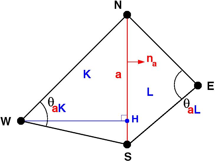
Figure 3: Co-boundary of the edge $\,a\in\mathcal{T}^{1}$.

Corollary 1.

Assume that the mesh satisfies the Delaunay condition: for all internal edge $a\in\mathcal{T}^{1}$ we have the angle condition $\theta_{a,K}+\theta_{a,L}<\pi$ (denoting $\partial^{c}a=(K,L)$). Also assume that for any boundary edge $a$, $\theta_{a,K}<\pi/2$ (denoting $\partial^{c}a=(K)$).
Then with (25), $(\varphi_{a}^{\star},\varphi_{a})_{0}>0$ and proposition 2 ensures the existence and uniqueness of the solution to the discrete problem. Moreover, the mixed Petrov-Galerkin discrete problem (17) for the Laplace equation (14) coincides with the four point finite volume scheme defined and analysed in Herbin [22].

Therefore, the Raviart-Thomas dual basis does not need to be constructed. Whatever are $\delta_{K}$ and $g$ that satisfy equations (18), (19) and (20), the coefficients $(\varphi_{a}^{\star},\varphi_{a})_{0}$ will be unchanged. They only depend on the mesh geometry and are given by equation (25). Practically, this means that neither the $\left(\varphi_{a}^{\star}\right)_{a\in\mathcal{T}^{1}}$ nor $\delta_{K}$ and $g$ need to be computed. Such a dual basis will be explicitly computed in section 5.1. The numerical scheme will always coincide with the four point volume scheme. Finally, this theorem provides a new point of view for the understanding and analysis of finite volume methods.
Theorem 1 gives sufficient conditions in order to build Raviart-Thomas dual basis. In the sequel we will focus on such Raviart-Thomas dual basis, though more general ones may exist: this will not be discussed in this paper.

Proof of corollary 1.

We have the general formula $\operatorname{cotan}\theta_{1}+\operatorname{cotan}\theta_{2}=\sin(\theta_{1}+\theta_{2})/(\sin\theta_{1}\,\sin\theta_{2})$ that ensures that $(\varphi_{a}^{\star},\varphi_{a})_{0}>0$ under the assumptions in the corollary.
For the equivalence between the two schemes, it suffices to prove that $\operatorname{cotan}\theta_{a,K}/2=d_{a,K}/|a|$ where $d_{a,K}$ denotes the distance between the edge $a$ and the circumcircle centre $C$ of $K$. Denote $S$ and $N$ the two vertexes of $a$. Then the angle $\widehat{SCN}=2\theta_{a,K}$. The distance $d_{a,K}$ is equal to $CH$ with $H$ the orthogonal projection of $C$ on $a$. The triangle $SCN$ being isosceles, $H$ is also the midle of $[SN]$. In the right angled triangle $SCH$ we have $\widehat{SCH}=\widehat{SCN}/2=\theta_{a,K}$ and $\operatorname{cotan}\widehat{SCH}=CH/SH=d_{a,K}/(|a|/2)$ which gives the result. $\blacksquare$

Proof of theorem 1.

Consider as in theorem 1 a family $(\varphi^{\star}_{K,i})_{K\in\mathcal{T}^{2},\,i=1,\,2,\,3}$ that satisfy, (22), (23) and (24) for $\delta_{K}$ and $g_{K,i}$ such that the assumptions (18), (19) and (20) are true. Let $\left(\varphi_{a}^{\star}\right)_{a\in\mathcal{T}^{1}}$ be constructed from the local basis functions $(\varphi^{\star}_{K,i})_{K,i}$ with equation (21).
Let us first prove that $\left(\varphi_{a}^{\star}\right)_{a\in\mathcal{T}^{1}}$ is a Raviart-Thomas dual basis as in definition 1. Consider an internal edge $a\in\mathcal{T}^{1}$, $a=(K|L)$. With (24), we have $\operatorname{supp}\varphi_{a}^{\star}=K\cup L$ and relation (7) holds. With (21), $\varphi^{\star}_{a\,|K}=\varphi^{\star}_{K,a}\in H(\operatorname{div},K)$, $\varphi^{\star}_{a\,|L}=-\varphi^{\star}_{L,a}\in H(\operatorname{div},L)$. The normal flux $\varphi_{a}^{\star}\cdot n_{a}$ is continuous across $a=K\cap L$ since $g_{K,a}=g_{L,a}$ and with (24). Moreover, $\varphi_{a}^{\star}\cdot n=0$ on the boundary of $K\cup L$ due to (24). Therefore $\varphi_{a}^{\star}$ belongs to $H(\operatorname{div},\Omega)$. With formula (25) and the angle condition made in theorem 1, $(\varphi_{a},\varphi_{a}^{\star})_{0}\neq 0$ and so (4) holds.
Consider two distinct edges $a,b\in\mathcal{T}^{1}$. If $a$ and $b$ are not two edges of a same triangle $K\in\mathcal{T}^{2}$, then $\varphi_{a}^{\star}$ and $\varphi_{b}$ have distinct supports so that $(\varphi_{a}^{\star},\varphi_{b})_{0}=0$. If $a$ and $b$ are two edges of $K\in\mathcal{T}^{2}$, then $(\varphi_{a}^{\star},\varphi_{b})_{0}=\int_{K}\varphi_{a}^{\star}\cdot\varphi_{b}\,\,{\rm d}x$. With the definition (1) of the local $RT$ basis functions and using the Green formula,

$$\pm 4|K|(\varphi_{a}^{\star},\varphi_{b})_{0} =-\int_{K}\operatorname{div}\varphi_{a}^{\star}\,|x-W_{K,b}|^{2}\,{\rm d}x+\int_{\partial K}\varphi_{a}^{\star}\cdot n|s-W_{K,b}|^{2}\,{\rm d}s$$

$$=-\int_{K}\delta_{K}\,|x-W_{K,b}|^{2}\,{\rm d}x+\int_{0}^{1}g(s)\,s^{2}\,ds,$$

using (23), (24) and the fact that $W_{K,b}$ is opposite to $b$ and so is a vertex of $a$. This implies the orthogonality condition (5) with the assumptions in (18) and (20).
It remains to prove (9). In the case where $a,b\in\mathcal{T}^{1}$ are two distinct edges, $\int_{b}\varphi_{a}^{\star}\cdot n_{b}\,{\rm d}s=0$. Assume that $a\in\mathcal{T}^{1}$ is an edge of $K\in\mathcal{T}^{2}$. We have $n_{a}=\varepsilon n_{K,a}$ with $\varepsilon=\pm 1$. With relation (24) and the divergence formula,

$$\int_{a}\varphi_{a}^{\star}\cdot n_{a}\,\,{\rm d}s=\int_{a}(\varepsilon\varphi_{K,a}^{\star})\cdot(\varepsilon n_{K,a})\,\,{\rm d}s=\int_{\partial K}\varphi_{K,a}^{\star}\cdot n\,\,{\rm d}s=\int_{K}\operatorname{div}\varphi_{K,a}^{\star}\,\,{\rm d}x.$$

This ensures that $\int_{a}\varphi_{a}^{\star}\cdot n_{a}\,ds=1$ with relation (23) and the first assumption in (20). We successively proved (4), (5), (7) and (9) and then $\left(\varphi_{a}^{\star}\right)_{a\in\mathcal{T}^{1}}$ is a Raviart-Thomas dual basis.
Let us now prove (25). Let $a\in\mathcal{T}^{1}$ an internal edge with the notations in figure 3. The Raviart-Thomas basis function $\varphi_{a}$ has its support in $K\cup L$, so that

$$(\varphi_{a}^{\star},\varphi_{a})_{0}=\int_{K}\varphi_{a}^{\star}\cdot\varphi_{a}\,{\rm d}x+\int_{L}\varphi_{a}^{\star}\cdot\varphi_{a}\,{\rm d}x.$$

With the local decompositions (2) and (21) we have,

$$(\varphi_{a}^{\star},\varphi_{a})_{0}=\int_{K}\varphi_{K,a}^{\star}\cdot\varphi_{K,a}\,\,{\rm d}x+\int_{L}\varphi_{L,a}^{\star}\cdot\varphi_{L,a}\,\,{\rm d}x\,.$$

By relation (1), $W$ being the opposite vertex to the edge $a$ in the triangle $K$,

$$4|K|\int_{K}\varphi_{K,a}^{\star}\cdot\varphi_{K,a}\,\,{\rm d}x = \int_{K}\varphi_{K,a}^{\star}\,\nabla|x-W|^{2}\,{\rm d}x$$

$$= -\int_{K}\operatorname{div}\varphi_{K,a}^{\star}\,|x-W|^{2}\,{\rm d}x+\int_{\partial K}\varphi_{K,a}^{\star}\cdot n_{K}\,|x-W|^{2}\,{\rm d}\sigma.$$

By hypothesis (23) and (24), and using (20),

$$4|K|\int_{K}\varphi_{K,a}^{\star}\cdot\varphi_{K,a}\,\,{\rm d}x =\int_{K}\delta_{K}|x-W|^{2}\,{\rm d}x+\int_{a}g_{K,a}\,|x-W|^{2}\,{\rm d}\sigma=\int_{a}g_{K,a}\,|x-W|^{2}\,{\rm d}\sigma.$$

Let H be the orthogonal projection of the point $W$ on the edge $a$. We have $|x-W|^{2}=WH^{2}+|x-H|^{2}$ and with (18) and (19), $\int_{a}g_{K,a}\,{\rm d}\sigma=|a|\int_{0}^{1}g(s)/|a|\,{\rm d}s=1$ and so,

$\displaystyle 4|K|\int_{K}\varphi_{K,a}^{\star}\cdot\varphi_{K,a}\,\,{\rm d}x=WH^{2}+\int_{a}g_{K,a}|x-H|^{2}\,{\rm d}\sigma.$

Let $s$ and $s^{\star}$ respectively be the curvilinear coordinates of $x$ and $H$ on $a$ with origin $S$, then

$\displaystyle 4|K|\int_{K}\varphi_{K,a}^{\star}\cdot\varphi_{K,a}\,\,{\rm d}x=WH^{2}+|a|^{2}\int_{0}^{1}(s^{\star}-s)^{2}g(s)ds.$

The assumptions in (18) on $g$ imply that $2\int_{0}^{1}g(s)sds=1$. By expanding $(s^{\star}-s)^{2}=s^{2}-2ss^{\star}+s^{\star\,2}$ we get, $\int_{0}^{1}(s^{\star}-s)^{2}g(s)ds=s^{\star\,2}-s^{\star}$. It follows that,

$$4|K|\int_{K}\varphi_{K,a}^{\star}\cdot\varphi_{K,a}\,\,{\rm d}x =WH^{2}+\bigl{(}|a|s^{\star}\bigl{)}\bigl{(}|a|(s^{\star}-1)\bigl{)}$$

$$=WH^{2}+\overrightarrow{SH}\cdot\overrightarrow{NH}$$

$$=\overrightarrow{WS}\cdot\overrightarrow{WN}.$$

Some trigonometry results in $K$ leads to $\sin\theta_{K,a}=\frac{2|K|}{WS\cdot WN}$. As a result,

$$4|K|\int_{K}\varphi_{K,a}^{\star}\cdot\varphi_{K,a}\,{\rm d}x=2|K|\,\operatorname{cotan}\theta_{K,a},$$

this gives (25). $\blacksquare$

5 Stability and convergence

In this section we develop a specific choice of dual basis functions. We provide for that choice technical estimates and prove a theorem of stability and convergence. With theorem 1, this leads to an error estimate for the four point finite volume scheme. We begin with the main result in theorem 2. Theorem 3 provides a methodology in order to get the inf-sup stability conditions. The inf-sup conditions need technical results that are proved in subsections 5.1 to 5.2. We will need the following angle condition.
Angle assumption. Let $\theta_{\star}$ and $\theta^{\star}$ chosen such that

$$0<\theta_{\star}<\theta^{\star}<\pi/2$$ (26)

We consider meshes $\mathcal{T}$ such that all the angles of the mesh are bounded from below and above by $\theta_{\star}$ and $\theta^{\star}$ respectively:

$$\forall\leavevmode\nobreak\ \theta\in\mathcal{T}^{-1},\quad\theta_{\star}\leq\theta\leq\theta^{\star}.$$ (27)

With that angle condition, the coefficients $(\varphi_{a},\varphi_{a}^{\star})$ in (25) are strictly positive. With proposition 2 this ensures the existence and uniqueness for the solution $(u_{\mathcal{T}},p_{\mathcal{T}})$ of the mixed Petrov-Galerkin discrete problem (15).

Theorem 2 (Error estimates).

We assume that $\Omega\subset\mathbb{R}^{2}$ is a bounded polygonal convex domain and that $f\in{\rm H}^{1}(\Omega)$. Under the angle hypotheses (26) and (27), there exists a constant $C$ independent on $\mathcal{T}$ satisfying (27) and independent on $f$ so that the solution $(u_{\mathcal{T}},p_{\mathcal{T}})$ of the mixed Petrov-Galerkin discrete problem (15) satisfies,

$$\|u_{\mathcal{T}}\|_{0}+\|p_{\mathcal{T}}\|_{{\rm H}(\operatorname{div},\Omega)}\leq C\|f\|_{0}.$$

Let $u$ be the exact solution to problem (14) and $p=\nabla u$ the gradient, the following error estimates holds,

$$\|u-u_{\mathcal{T}}\|_{0}+\|p-p_{\mathcal{T}}\|_{{\rm H}(\operatorname{div},\Omega)}\leq Ch_{\mathcal{T}}\|f\|_{1},$$ (28)

with $h_{\mathcal{T}}$ the maximal size of the edges of the mesh.

Proof.

We prove that the unique solution of the mixed Petrov-Galerkin (15) continuously depends on the data $f$. The bilinear form $Z$ defined in (16) is continuous, with a continuity constant $M$ independent on the mesh $\mathcal{T}$,

$$|Z(\xi,\eta)|\,\,\leq\,\,M\,\,\|\xi\|_{{\rm L}^{2}\times{\rm H}_{\operatorname{div}}}\,\|\eta\|_{{\rm L}^{2}\times{\rm H}_{\operatorname{div}}}\,,\qquad\forall\,\xi\in V,\,\eta\in V^{\star}.$$

The following uniform inf-sup stability condition: there exists a constant $\beta>0$ independent on $\mathcal{T}$ such that,

$$\forall\leavevmode\nobreak\ \xi\in V,\,{\rm so\,that}\,\,\|\xi\|_{{\rm L}^{2}\times{\rm H}_{\operatorname{div}}}=1,\,\exists\leavevmode\nobreak\ \eta\in V^{\star},\,\,\|\eta\|_{{\rm L}^{2}\times{\rm H}_{\operatorname{div}}}\,\leq\,1\,\,{\rm and}\,\,Z(\xi,\eta)\,\geq\,\beta,$$ (29)

is proven in theorem 3 under some conditions. Moreover, the two spaces $V$ and $V^{\star}$ have the same dimension. Then the Babuška theorem in [6], also valid for Petrov-Galerkin mixed formulation, applies. The unique solution $\xi_{{}_{\cal T}}=(u_{{}_{\mathcal{T}}},p_{{}_{\mathcal{T}}})$ of the discrete scheme (15) satisfies the error estimates, and

$$\|\xi-\xi_{{}_{\cal T}}\|_{{\rm L}^{2}\times{\rm H}_{\operatorname{div}}}\,\,\,\leq\,\,\,\Big{(}1+\frac{M}{\beta}\Bigr{)}\inf_{\zeta\in V}\|\xi-\zeta\|_{{\rm L}^{2}\times{\rm H}_{\operatorname{div}}}\,,$$

with $\xi=(u,p)$, $u$ the exact solution to the Poisson problem (14) and $p=\nabla u$. In our case, this formulation is equivalent to

$$\|u-u_{{}_{\cal T}}\|_{0}\,+\,\|p-p_{{}_{\cal T}}\|_{{\rm H}(\operatorname{div},\Omega)}\,\leq\,C\,\Big{(}\inf_{v\in P^{0}}\,\|u-v\|_{0}+\inf_{q\in RT}\|p-q\|_{{\rm H}(\operatorname{div},\Omega)}\Big{)}$$ (30)

for a constant $C=1+\frac{M}{\beta}$ dependent of $\mathcal{T}$ only through the lowest and the highest angles $\theta_{\star}$ and $\theta^{\star}$. With the interpolation operators $\Pi_{0}:{\rm L}^{2}(\Omega)\rightarrow P^{0}$ and $\Pi_{RT}:{\rm H}^{1}(\Omega)^{2}\rightarrow RT^{0}$

$$\|\,u-u_{{}_{\cal T}}\,\|_{0}\,+\,\|\,p-p_{{}_{\cal T}}\,\|_{{\rm H}(\operatorname{div},\Omega)}\,\leq\,C\,\big{(}\|\,u-\Pi_{0}u\,\|_{0}+\|\,p-\Pi_{\text{\tiny RT}}p\,\|_{{\rm H}(\operatorname{div},\Omega)}\big{)}.$$

On the other hand we have the following interpolation errors:

$$\|\,u-\Pi_{0}u\,\|_{0}\,\leq\,C_{1}h_{\cal T}\,\|u\,\|_{1},\,\quad\|\,p-\Pi_{\text{\tiny RT}}p\,\|_{0}\,\leq C_{2}\,h_{\cal T}\,\|p\,\|_{1},\,\quad\|\operatorname{div}\big{(}p-\Pi_{\text{\tiny RT}}p\big{)}\|_{0}\leq C_{1}h_{\cal T}\,\|\operatorname{div}p\,\|_{1}.$$

On the left, we have the Poincaré-Wirtinger inequality where the constant $C_{1}=1/\pi$ is independent on the mesh, due to [28]. The third inequality is the same as the first one since $\Pi_{0}\operatorname{div}p=\operatorname{div}\Pi_{\text{\tiny RT}}p$. For the second inequality, the constant $C_{2}$ has been proven in [3] to be dominated by $1/\sin\theta^{\star}$ with $\theta^{\star}$ the maximal angle of the mesh.
Then ,

$$\|\,u-u_{{}_{\cal T}}\,\|_{0}\,+\,\|\,p-p_{{}_{\cal T}}\,\|_{{\rm H}(\operatorname{div},\Omega)}\,\leq\,C\,h_{\cal T}\,\big{(}\,\|u\,\|_{1}+\|p\,\|_{1}+\|\operatorname{div}p\,\|_{0}\,\big{)}\,,$$

with a constant $C$ only depending on the maximal angle $\theta^{\star}$. Since $-\Delta u=f\,\,\,{\rm in}\,\Omega$, with $f\in{\rm H}^{1}(\Omega)$ and $\Omega$ convex, then $u\in{\rm H}^{2}(\Omega)$ and $\|u\|_{2}\leq c\|f\|_{0}$. Moreover $p=\nabla u$ and $\operatorname{div}p=-f$ leads to

$$\|\,u-u_{{}_{\cal T}}\,\|_{0}\,+\,\|\,p-p_{{}_{\cal T}}\,\|_{{\rm H}(\operatorname{div},\Omega)}\,\leq\,C\,h_{\cal T}\,\big{(}2\|f\,\|_{0}+\|f\,\|_{1}\big{)}\,.$$

Finally, we get

$$\|\,u-u_{{}_{\mathcal{T}}}\,\|_{0}\,+\,\|\,p-p_{{}_{\cal T}}\,\|_{{\rm H}(\operatorname{div},\Omega)}\,\leq\,C\,h_{\mathcal{T}}\,\|\,f\,\|_{1}\,,$$

that is exactly (28). $\blacksquare$

Theorem 3 (Abstract stability conditions).

Assume that the projection $\Pi:\leavevmode\nobreak\ RT\rightarrow RT^{\star},$ such that $\Pi\varphi_{a}=\varphi_{a}^{\star}$ in diagram (6) satisfies, for any $p\in RT$:

$$(p,\Pi p)_{0}\, \geq\,A\,\|p\|_{0}^{2},$$ (H1)

$$\|\Pi p\|_{0} \leq B\,\|p\|_{0},$$ (H2)

$$(\operatorname{div}p,\operatorname{div}\Pi p)_{0}\, \geq\,C\,\|\operatorname{div}p\|_{0}^{2},$$ (H3)

$$\|\operatorname{div}\Pi p\|_{0}\, \leq\,D\,\|\operatorname{div}p\|_{0}$$ (H4)

where $A,\,B,\,C,\,D>0$ are constants independent on $\mathcal{T}$. Then the uniform discrete inf-sup condition (29) holds: there exists a constant $\beta>0$ independent on $\mathcal{T}$ such that,

$$\forall\leavevmode\nobreak\ \xi\in V,\,{\rm so\,that}\,\,\|\xi\|_{{\rm L}^{2}\times{\rm H}_{\operatorname{div}}}=1,\,\exists\leavevmode\nobreak\ \eta\in V^{\star},\,\,\|\eta\|_{{\rm L}^{2}\times{\rm H}_{\operatorname{div}}}\,\leq\,1\,\,{\rm and}\,\,Z(\xi,\eta)\,\geq\,\beta.$$

This result has been proposed by Dubois in [15]. For the completeness of this contribution, the proof (presented in the preprint [16]) is detailed in Annex A.

In order to prove the conditions (H1), (H2), (H3) and (H4), one needs some technical lemmas on some estimations of the dual basis functions so that theorem 3 holds. It is the goal of the next subsections.

5.1 A specific Raviart-Thomas dual basis

Choice of the divergence

For $K$ a given triangle of $\mathcal{T}^{2}$, we propose a choice for the divergence $\delta_{K}$ of the dual basis functions $\varphi_{K,i}^{\star},\,1\leq i\leq 3$ in (23). We know from (20) that this function has to be ${\rm L}^{2}(K)$-orthogonal to the three following functions: $|x-W_{K,i}|^{2}$ for $i=$1, 2, 3 and that its integral over $K$ is equal to 1. We propose to choose $\delta_{K}$ as the solution of the least-square problem: minimise $\int_{K}\delta_{K}^{2}\,\,{\rm d}x$ with the constraints in (20). It is well-known that the solution belongs to the four dimensional space $E_{K}=\operatorname{span}\left(1{\rm l}_{K},|x-W_{K,i}|^{2},\leavevmode\nobreak\ 1\leq i\leq 3\right)$ and is obtained by the inversion of an appropriate Gram matrix.

Lemma 1.

For the above construction of $\delta_{K}$, we have the following estimation:

$$|K|\int_{K}\delta_{K}^{2}\,{\rm d}x\leq\nu,\qquad\text{with}\quad\nu=\frac{8\cdot 3^{5}\cdot 23}{5}\,\,{\frac{1}{\tan^{4}\theta_{\star}}}.$$

The proof of this result is technical and has been obtained with the help of a formal calculus software. It is detailed in Annex C.

Choice of the flux on the boundary of the triangle

A continuous function $g:(0,1)\rightarrow\mathbb{R}$ satisfying the conditions (18) can be chosen as the following polynomial:

$$g(s)=30s\,(s-1)\,(21s^{2}-21s+4).$$ (31)

Construction of the Raviart-Thomas dual basis

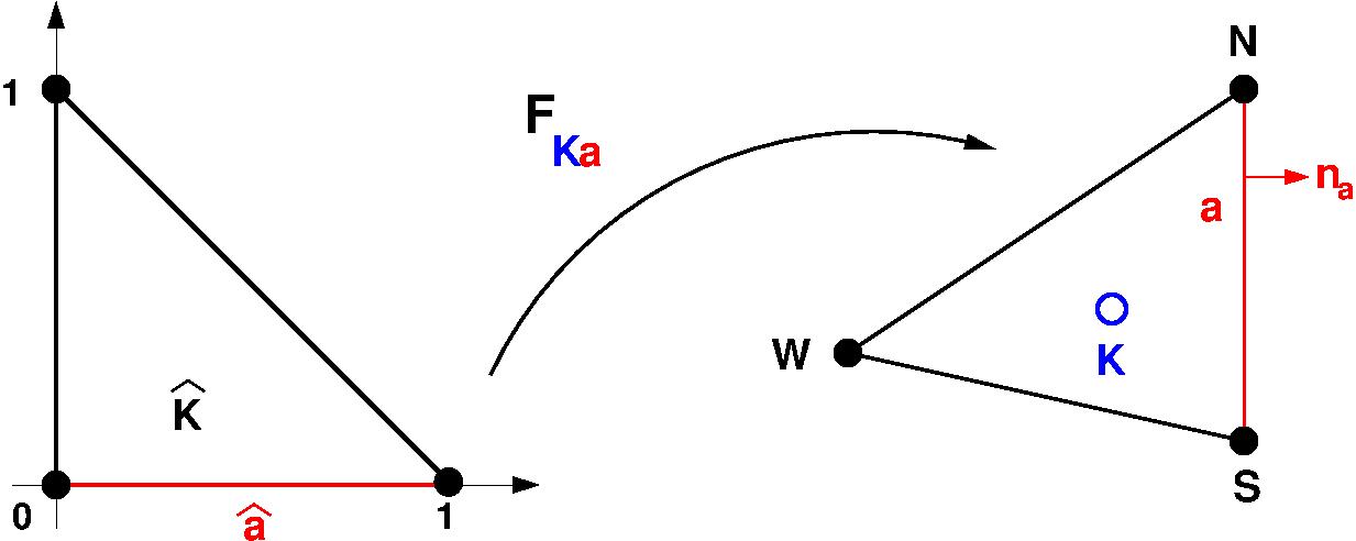
Figure 4: Affine mapping $\,F_{K,a}\,$ between the reference triangle $\,\hat{K}\,$ and the given triangle $\,K$.

For a triangle $K$ and an edge $a$ of $K$, we construct now a possible choice of the dual function $\varphi_{K,a}^{\star}$ satisfying (22), (23) and (24). Let $\,F_{K,a}\,$ be an affine function that maps the reference triangle $\hat{K}$ into the triangle $\,K\,$ such that the edge $\,\hat{a}\equiv[0,1]\times\{0\}\,$ is transformed into the given edge $\,a\subset\partial K$. Then the mapping $\,\,\widehat{K}\ni\widehat{x}\longmapsto x=F_{K,a}(\widehat{x})\in K$ is one to one. We define $x=F_{K,a}(\hat{x})$ for any $\hat{x}\in\hat{K}$ and the right hand side $\,\,\widetilde{\delta}_{K}(\hat{x})=2\,|K|\,\delta_{K}(x)$. With $g$ defined in (31), let us define $\,\widehat{g}\in{\rm H}^{1/2}(\partial\hat{K})\,$ according to

$\displaystyle\widehat{g}:=\left\{\begin{array}[]{ll}g\text{ on }\hat{a}=[0,1]\times\{0\}\\ 0\text{ elsewhere on }\partial\hat{K}\,.\end{array}\right.$

Since  $\displaystyle\int_{\widehat{K}}\widetilde{\delta_{K}}\,\,{\rm d}x\,=1\,=\,\int_{\partial\hat{K}}\widehat{g}\,\,{\rm d}\gamma$, the inhomogeneous Neumann problem

$$\Delta\zeta_{K}=\widetilde{\delta}_{K}\,\,\text{ in }\hat{K}\,,\quad\frac{\partial\zeta_{K}}{\partial n}=\widehat{g}\,\,\text{ on }\partial\hat{K}$$ (32)

is well posed. The dual function $\,\varphi_{K,a}^{\star}\,$ is defined according to

$$\varphi_{K,a}^{\star}(x)={\frac{1}{\det({\rm d}F_{K,a})}}\,{\rm d}F_{K,a}\,\,\widehat{\nabla}\zeta_{K}\,.$$ (33)

These so-defined functions satisfy the hypotheses (22), (23) and (24) of theorem 1. Let us now estimate their ${\rm L}^{2}$-norm.

${\rm L}^{2}$-norm of the Raviart-Thomas dual basis

An upper bound on the ${\rm L}^{2}$ norm of the Raviart-Thomas dual basis will be needed in order to prove the stability conditions in theorem 3. This bound is given in lemma 3. It only involves the mesh minimal angle $\theta_{\star}$.

Lemma 2.

For $K\in\mathcal{T}^{2}$ and $a\in\mathcal{T}^{1}$, $\,a\subset\partial K$, we have

$\displaystyle\|\varphi_{K,\,a}^{\star}\|_{0\,K}\,\leq\,\mu^{\star}$

where $\mu^{\star}$ is essentially a function of the smallest angle $\theta_{\star}$ of the triangulation.

Proof.

Since the reference triangle $\,\hat{K}\,$ is convex and $\,\widehat{g}\in{\rm H}^{1/2}(\partial\widehat{K})$, the solution $\zeta_{K}$ of the Neumann problem (32) satisfies the regularity property (see for example [4]) $\,\zeta_{K}\in{\rm H}^{2}(\widehat{K})$, continuously to the data:

$\displaystyle\displaystyle\|\zeta_{K}\|_{2,\hat{K}}\,\leq\,C_{\widehat{K}}\,\Big{(}\,\|\widetilde{\delta_{K}}\|_{0,\widehat{K}}+\|\widehat{g}\|_{1/2,\,\partial\widehat{K}}\,\Big{)}\,.$

Moreover thanks to lemma 1,

$\displaystyle\|\widetilde{\delta_{K}}\|_{0,\hat{K}}^{2}=\int_{\widehat{K}}\widetilde{\delta_{K}}^{2}\,{\rm d}\widehat{x}=\int_{K}\,(2|K|\delta_{K})^{2}\,\frac{1}{\det({\rm d}F_{K,a})}\,{\rm d}x=2\,|K|\int_{K}\delta_{K}^{2}\,{\rm d}x\leq\,2\,\nu$

and then

$\displaystyle\|\widehat{\nabla}\zeta_{K}\|_{0,\hat{K}}\,\leq\,C_{\widehat{K}}\,\Big{(}\,\sqrt{2\nu}+\|\widehat{g}\|_{1/2,\,\partial\widehat{K}}\,\Big{)}\,.$

Since the dual function $\varphi_{K,a}^{\star}$ is defined by (33) and $\|{\rm d}F_{K,a}\|^{2}\leq\frac{8|K|}{\sin\theta_{\star}}$ from direct geometrical computations on the triangle $K$, we obtain

$$\|\varphi_{K,a}^{\star}\|_{0,K}^{2}\leq\displaystyle\Big{(}{\frac{1}{2\,|K|}}\Big{)}^{2}\,\Big{(}{\frac{8\,|K|}{\sin\,\theta_{\star}}}\Big{)}\,\|\widehat{\nabla}\zeta_{K}\|_{0,\hat{K}}^{2}\,(2\,|K|)\,.$$

Then $\displaystyle\|\varphi_{K,a}^{\star}\|_{0,K}^{2}\leq\displaystyle(\mu^{\star})^{2}\,,$ with $\displaystyle(\mu^{\star})^{2}={\frac{4}{\sin\,\theta_{\star}}}\,\,C_{\widehat{K}}^{2}\,\Big{(}\,\sqrt{2\nu}+\|\widehat{g}\|_{1/2,\,\partial\widehat{K}}\,\Big{)}^{2}\,.$ $\blacksquare$

Lemma 3.

For $K\in\mathcal{T}^{2}$ and $q\in RT^{\star}$:

$$\|\Pi q\|_{0,K}^{2}\leq 3(\mu^{\star})^{2}\sum_{i=1}^{3}q_{K,i}^{2}\,\,.$$

Proof.

We have for a triangle $K$, $\displaystyle\Pi q=\sum_{i=1}^{3}q_{K,i}\varphi^{\star}_{K,i}$, and so

$$\|\Pi q\|_{0,K}^{2}\leq\Big{(}\sum_{i=1}^{3}|q_{K,i}|\,\|\varphi^{\star}_{K,i}\|_{0,K}\Big{)}^{2}\leq\sum_{i=1}^{3}|q_{K,i}|^{2}\sum_{i=1}^{3}\|\varphi^{\star}_{K,i}\|_{0,K}^{2}$$

Then lemma 2 applies and: $\displaystyle\|\Pi q\|_{0,K}^{2}\leq 3(\mu^{\star})^{2}\sum_{i=1}^{3}q_{K,i}^{2}\,.$ $\blacksquare$

5.2 Local Raviart-Thomas mass matrix

The proof of the stability conditions in theorem 3 involves lower and upper bounds of the eigenvalues of the local Raviart-Thomas mass matrix. We will need the following result proved in Annex B.

Lemma 4.

For $p\in RT$ and $K\in\mathcal{T}^{2}$:

$\displaystyle\lambda_{\star}\,\sum_{i=1}^{3}p_{K,i}^{2}\,\leq\,\|p\|_{0,K}^{2}\,\leq\,\lambda^{\star}\,\sum_{i=1}^{3}p_{K,i}^{2},$

for two constants $\lambda_{\star}$ and $\lambda^{\star}$ only depending on $\theta_{\star}$ in (26),

$\displaystyle\lambda_{\star}=\frac{\tan^{2}\theta_{\star}}{48},\quad\lambda^{\star}=\frac{5}{4\tan\theta_{\star}}.$

5.3 The hypotheses of theorem 3 are satisfied

Let us finally prove that the conditions (H1), (H2), (H3) and (H4) of theorem 3 hold. The proof relies on lemma 4, lemma 3 and lemma 1 involving the mesh independent constants $\lambda_{\star}$, $\lambda^{\star}$, $\mu^{\star}$ and $\nu$. In the following, $p$ denotes an element of $RT$ and $K$ a fixed mesh triangle. It is recalled that on $K$, $\displaystyle p=\sum_{i=1}^{3}p_{K,i}\,\,\varphi_{K,i}$.

Condition (H1). Using the orthogonality property (5), and relation (25) successively, leads to

$$(\Pi p,p)_{0,K}=\sum_{i=1}^{3}p_{K,i}^{2}\,(\varphi^{\star}_{K,i},\varphi_{K,i})_{0,K}=\frac{1}{2}\sum_{i=1}^{3}p_{K,i}^{2}\,\operatorname{cotan}\theta_{K,i}\geq\frac{1}{2}\operatorname{cotan}\theta^{\star}\sum_{1=1}^{3}p_{K,i}^{2}.$$

Lemma 4 gives a lower bound,

$\displaystyle(\Pi p,p)_{0,K}\geq\frac{\operatorname{cotan}\theta^{\star}}{2\lambda^{\star}}\|p\|^{2}_{0,K}.$

Summation over all $K\in\mathcal{T}^{2}$ gives (H1) with,

$\displaystyle A=\frac{\operatorname{cotan}\theta^{\star}}{2\lambda^{\star}}=\frac{2}{5}\operatorname{cotan}\theta^{\star}\tan\theta_{\star}.$

Condition (H2). Using successively lemma 3 and lemma 4 we get,

$\displaystyle\|\Pi p\|_{0,K}^{2}\leq 3(\mu^{\star})^{2}\sum_{i=1}^{3}p_{K,i}^{2}\leq\frac{3(\mu^{\star})^{2}}{\lambda_{\star}}\|p\|_{0,K}^{2}.$

With the values of $\lambda_{\star}$ given in lemma 3 this implies (H2) with,

$\displaystyle B=\sqrt{\frac{3(\mu^{\star})^{2}}{\lambda_{\star}}}=\frac{12}{\tan\theta_{\star}}\mu^{\star}.$

Condition (H3). Relation (11) induces $(\operatorname{div}\Pi p,\operatorname{div}p)_{0,K}=\|\operatorname{div}p\|^{2}_{0,K}$ since $\operatorname{div}p$ is a constant on $K$, and as a result inequality (H3) indeed is an equality with

$$C=1.$$

Condition (H4). With equation (3) we get $\|\operatorname{div}p\|^{2}_{0,K}=\left(\sum_{1=1}^{3}p_{K,i}\right)^{2}/|K|$ and with condition (23), $\operatorname{div}\Pi p=\delta_{K}(x)\sum_{1=1}^{3}p_{K,i}$. Therefore we get,

$\displaystyle\|\operatorname{div}\Pi p\|^{2}_{0,K}=\int_{K}\delta_{K}^{2}\,{\rm d}x\leavevmode\nobreak\ \left(\sum_{1=1}^{3}p_{K,i}\right)^{2}=|K|\int_{K}\delta_{K}^{2}\,{\rm d}x\leavevmode\nobreak\ \|\operatorname{div}p\|^{2}_{0,K}.$

Condition (H4) follows from lemma 1, with

$\displaystyle D=\sqrt{\nu},\quad\nu=\frac{8\leavevmode\nobreak\ 3^{5}\leavevmode\nobreak\ 23}{5}\,\,{\frac{1}{\tan^{4}\theta_{\star}}}.$

Conclusion

In this contribution we present a way to define a local discrete gradient of a piecewise constant function on a triangular mesh. This discrete gradient is obtained from a Petrov-Galerkin formulation and belongs to the Raviart-Thomas function space of low order. We have defined suitable dual test functions of the Raviart-Thomas basis functions. For the Poisson problem, we can interpret the Petrov-Galerkin formulation as a finite volume method. Specific constraints for the dual test functions enforce stability. Then the convergence can be established with the usual methods of mixed finite elements. It would be interesting to try to extend this work in several directions: the three-dimensional case, the case of general diffusion problems and also the case of higher degree finite element methods.

Annex A Proof of theorem 3

In this section, we consider meshes $\mathcal{T}$ that satisfy the angle conditions (27) parametrised by the pair $\,0<\theta_{\star}<\theta^{\star}<{\frac{\pi}{2}}\,$. We suppose that the interpolation operator $\Pi$ defined in section 1 by $\,\Pi:RT\longrightarrow RT^{\star}\,$ with $\Pi\varphi_{a}=\varphi_{a}^{\star}$ satisfies the following properties: there exist four positive constants $A$, $B$, $C$ and $D$ only depending on $\theta_{\star}$ and $\theta^{\star}$ such that for all $q\in RT$

$$(q,\Pi q) \,\geq\, A\,\,\|q\|_{0}^{2}\,,$$ (34)

$$\|\Pi q\|_{0} \leq B\,\|q\|_{0}\,,$$ (35)

$$(\operatorname{div}q,\operatorname{div}\Pi q)_{0} \geq C\,\|\operatorname{div}q\|_{0}^{2}\,,$$ (36)

$$\|\operatorname{div}\Pi q\|_{0} \leq D\,\|\operatorname{div}q\|_{0}\,.$$ (37)

Let us first prove the following proposition relative to the lifting of scalar fields.

Proposition 3 (Divergence lifting of scalar fields).

Under the previous hypotheses (34), (35), (36) and (37), there exists some strictly positive constant $\,F\,$ that only depends of the minimal and maximal angles $\theta_{\star}$ and $\theta^{\star}$ such that for any mesh $\,{\mathcal{T}}\,$ and for any scalar field $\,u\,$ constant in each element $\,K$ of $\mathcal{T}$, ($u\,\in P^{0}$), there exists some vector field $\,\,q\,\in RT^{\star},\,$ such that

$$\centering\displaystyle\parallel q\parallel_{H_{\operatorname{div}}}\,\,\,\leq\,\,\,F\,\parallel u\parallel_{0}\vspace*{-6pt}\@add@centering$$ (38)

$$\centering\displaystyle(\,u\,,\,{\rm div}\,q\,)_{0}\quad\,\geq\,\,\,\,\parallel u\parallel_{0}^{2}\,\,.\,\vspace*{-6pt}\@add@centering$$ (39)

Proof.

Let $\,\,u\in\,P^{0}\,$ be a discrete scalar function supposed to be constant in each triangle $\,K\,$ of the mesh $\,{\mathcal{T}}.\,$ Let $\,\psi\,\in{\rm H}^{1}_{0}(\Omega)\,$ be the variational solution of the Poisson problem

$$\centering\displaystyle\Delta\,\psi\,\,=\,\,u\quad{\rm in}\,\,\Omega\,\,,\quad\psi\,=\,0\quad{\rm on}\,\,\partial\Omega\,.\,\vspace*{-6pt}\@add@centering$$ (40)

Since $\,\Omega\,$ is convex, the solution $\,\psi\,$ of the problem (40) belongs to the space $\,{\rm H}^{2}(\Omega)\,$ and there exists some constant $\,G>0\,$ that only depends on $\,\Omega\,$ such that

$$\parallel\psi\parallel_{2}\,\,\,\leq\,\,\,G\,\parallel u\parallel_{0}\,.$$

Then the field $\,\,\nabla\psi\,\,$ belongs to the space $\,{\rm H}^{1}(\Omega)\,\times\,{\rm H}^{1}(\Omega).\,$ It is in consequence possible to interpolate this field in a continuous way (see e.g. Roberts and Thomas [34]) in the space $\,{\rm H}({\rm div},\,\Omega)\,\,$ with the help of the fluxes on the edges:

$$p_{a}\,\,=\,\,\int_{\displaystyle a}\,{\frac{\partial\psi}{\partial n_{a}}}\,{\rm d}\gamma\,,\qquad p\,=\,\sum_{a\,\in\mathcal{T}^{1}}\,p_{a}\,\,\varphi_{a}\,\,\,\in\,\,RT\,.$$

Then there exists a constant $\,L>0\,$ such that

$$\centering\displaystyle\parallel p\parallel_{H_{\operatorname{div}}}\,\,\,\leq\,\,\,L\,\,\parallel u\parallel_{0}\,.\vspace*{-6pt}\@add@centering$$ (41)

The two fields $\,{\rm div}\,p\,$ and $\,u\,$ are constant in each element $\,K\,$ of the mesh $\,{\mathcal{T}}.\,$ Moreover, we have:

$$\centering\displaystyle\int_{K}\,{\rm div}\,p\,\,{\rm d}x\,\,=\,\,\int_{\partial K}\,p\,\cdot\,n\,\,{\rm d}\gamma\,\,=\,\,\int_{\partial K}\,{\frac{\partial\psi}{\partial n}}\,\,{\rm d}\gamma\,\,=\,\,\int_{K}\,\Delta\psi\,\,{\rm d}x\,\,=\,\,\int_{K}\,u\,\,{\rm d}x\,.\vspace*{-6pt}\@add@centering$$

Then we have exactly, $\,{\rm div}\,p\,=\,u\,$ in $\,\Omega\,$ because this relation is a consequence of the above property for the mean values.
Let now $\,\,\Pi\,p\,$ be the interpolate of $p$ in the “dual space” $\,RT^{\star}\,$ and $q\,\,=\,\,\frac{1}{C}\,\Pi\,p$,

$$\centering\displaystyle q\,\,=\,\,{\frac{1}{C}}\,\Pi\,p\,\,=\,\,{\frac{1}{C}}\,\sum_{a\in\mathcal{T}^{1}}p_{a}\,\varphi_{a}^{\star}\quad{\rm with}\quad\Pi\,p\,=\,\sum_{a\in\mathcal{T}^{1}}p_{a}\,\varphi_{a}^{\star}.\,\vspace*{-6pt}\@add@centering$$

We have as a consequence of (36) and $\,{\rm div}\,p=u$ that,

$$\centering\displaystyle(\,u\,,\,{\rm div}\,q\,)_{0}\,\,=\,\,{\frac{1}{C}}\,(\,{\rm div}\,p\,,\,{\rm div}\,\Pi\,p\,)\,\,\geq\,\,\parallel{\rm div}\,p\parallel_{0}^{2}\,\,\,=\,\,\,\parallel u\parallel_{0}^{2}\vspace*{-6pt}\@add@centering$$

that establishes (39). Moreover, we have due to equations (35), (37) and (41):

$$\parallel q\parallel_{0} \,=\, {\frac{1}{C}}\,\parallel\Pi\,p\parallel_{0}\,\leq\,{\frac{B}{C}}\,\parallel p\parallel_{0}\,\leq\,{\frac{BL}{C}}\,\parallel u\parallel_{0}\,,$$

$$\parallel{\rm div}\,q\parallel_{0} \,=\, {\frac{1}{C}}\,\parallel{\rm div}\,\Pi\,p\parallel_{0}\,\leq\,{\frac{D}{C}}\,\parallel{\rm div}\,p\parallel_{0}\,=\,{\frac{D}{C}}\,\parallel u\parallel_{0}\,.$$

Then the two above inequalities establish the estimate (38) with $\,\,F\,=\,{\frac{1}{C}}\,\sqrt{B^{2}{\rm L}^{2}+D^{2}}\,\,$ and the proposition is proven. $\blacksquare$

Proof of theorem 3

We suppose that the dual Raviart-Thomas basis satisfies the Hypothesis (34) to (37). We introduce the constant $\,F>0\,$ such that (38) and (39) are realised for some vector field $\,\widetilde{q}\in RT^{\star}\,$ for any $\,u\in P^{0}$:

$$\centering\displaystyle\parallel\widetilde{q}\parallel_{H_{\operatorname{div}}}\,\,\,\leq\,\,\,F\,\parallel u\parallel_{0}\quad{\rm and}\quad(\,u\,,\,{\rm div}\,\widetilde{q}\,)_{0}\,\,\geq\,\,\parallel u\parallel_{0}^{2}\,\,.\vspace*{-6pt}\@add@centering$$ (42)

$\bullet$  We set $\,\displaystyle a={\frac{1}{2}}\big{(}\sqrt{4+F^{2}}-F\big{)},\,$ $\,\displaystyle b={\frac{A}{D+\sqrt{B^{2}+D^{2}}}}\,$ with the constants $\,F$, $\,A$, $\,B\,$ and $\,D\,$ introduced in (42), (34), (35) and (37) respectively. We shall prove that for

$$\centering\displaystyle\beta={\frac{b\,a^{2}}{1+2\,a\,b}}\,,\vspace*{-6pt}\@add@centering$$ (43)

the inf-sup condition

$$\centering\displaystyle\left\{\begin{array}[]{ll}\exists\,\beta>\,0\,,\,\,\,\,,\,\,\forall\,\xi\,\in P^{0}\times RT\,\,$ such that $\displaystyle\,\,\,\,\parallel\xi\parallel_{{\rm L}^{2}\times{\rm H}_{\operatorname{div}}}\,\,=\,\,1\,,\\ \exists\,\eta\,\in\,P^{0}\times RT^{\star}\,,\,\,\parallel\eta\parallel_{{\rm L}^{2}\times{\rm H}_{\operatorname{div}}}\,\,\leq\,\,1\,\,\,{\rm and}\,\,\,Z(\xi,\,\eta)\,\,\geq\,\,\beta\end{array}\right.\vspace*{-6pt}\@add@centering$$ (44)

is satisfied. We set

$$\centering\displaystyle\alpha\equiv a-\beta=a{\frac{1+a\,b}{1+2\,a\,b}}>0\,.\vspace*{-6pt}\@add@centering$$ (45)

Then we have after an elementary algebra: $\,\,\,a\,F+a^{2}=1.\,$ In consequence,

$$\centering\displaystyle(\alpha+\beta)\,F+\alpha^{2}+\beta^{2}\,\leq\,1\vspace*{-6pt}\@add@centering$$ (46)

because $\displaystyle\,(\alpha+\beta)\,F+\alpha^{2}+\beta^{2}\,\leq\,(\alpha+\beta)\,F+(\alpha+\beta)^{2}=1$. Moreover,

$$\centering\displaystyle\beta\leq b\,\alpha^{2}\vspace*{-6pt}\@add@centering$$ (47)

thanks to the relations (43) and (45):

$$\beta-b\,\alpha^{2}={\frac{1}{(1+2\,a\,b)^{2}}}\,\Big{[}b\,a^{2}\,(1+2\,a\,b)-b\,a^{2}\,(1+a\,b)^{2}\Big{]}=-{\frac{a^{4}\,b^{3}}{(1+2\,a\,b)^{2}}}.$$

$\bullet$  Consider now $\,\,\xi\equiv(u,\,p)\,\,$ satisfying the hypothesis of unity norm in the product space:

$$\centering\displaystyle\parallel\xi\parallel_{{\rm L}^{2}\times{\rm H}_{\operatorname{div}}}\,\,\,\,\equiv\,\,\,\parallel u\parallel_{{}_{\scriptstyle{0}}}^{2}\,\,+\,\,\parallel p\parallel_{{}_{\scriptstyle{0}}}^{2}\,\,+\,\,\parallel{\rm div}\,p\parallel_{{}_{\scriptstyle{0}}}^{2}\,\,\,=\,\,\,1\,.\,\vspace*{-6pt}\@add@centering$$ (48)

Then at last one of these terms is not too small and due to the three terms that arise in relation (48), the proof is divided into three parts.

(i) If the condition $\displaystyle\,\,\parallel{\rm div}\,p\parallel_{{}_{\scriptstyle{0}}}\,\,\geq\,\,\beta\,\,$ is satisfied, we set

$$\centering\displaystyle v\,\,=\,\,{\frac{{\rm div}\,p}{\parallel{\rm div}\,p\parallel_{{}_{\scriptstyle{0}}}}}\,\,,\quad q\,\,=\,\,0\,\,,\qquad\eta\,\,=\,\,(v,\,q)\,.\vspace*{-6pt}\@add@centering$$

Then, $\,\,\,\displaystyle\parallel{\rm div}\,v\parallel_{{}_{\scriptstyle{0}}}\,=\,1\,\,\,\,$ and $\,\,\,\displaystyle\parallel\eta\parallel_{{}_{\scriptstyle{0}}}\,\leq\,1\,.\,$ Moreover

$$\centering\displaystyle Z(\xi,\,\eta)\,=\,(\,{\rm div}\,p\,,\,v\,)_{0}\,\,=\,\,\parallel{\rm div}\,p\parallel_{{}_{\scriptstyle{0}}}\,\,\geq\,\,\beta\vspace*{-6pt}\@add@centering$$

and the relation (44) is satisfied in this particular case.

(ii) If the conditions $\displaystyle\,\,\parallel{\rm div}\,p\parallel_{{}_{\scriptstyle{0}}}\,\,\leq\,\,\beta\,\,$ and $\displaystyle\parallel p\parallel_{{}_{\scriptstyle{0}}}\,\,\geq\,\,\alpha\,\,$ are satisfied, we set

$$\centering\displaystyle v\,\,=\,\,0\,\,\,\,,\quad q\,\,=\,\,{\frac{1}{\sqrt{B^{2}+D^{2}}}}\,\,\Pi\,p\,\,,\qquad\eta\,\,=\,\,(v,\,q)\,.\vspace*{-6pt}\@add@centering$$

We check that $\|\eta\|_{{\rm L}^{2}\times{\rm H}_{\operatorname{div}}}\leq 1$:

$$\|\eta\|_{{\rm L}^{2}\times{\rm H}_{\operatorname{div}}}^{2} \,=\, \parallel q\parallel_{{}_{\scriptstyle{0}}}^{2}+\parallel{\rm div}\,q\parallel_{{}_{\scriptstyle{0}}}^{2}\,\,\leq\,\,{\frac{1}{B^{2}+D^{2}}}\,\Big{(}B^{2}\,\parallel p\parallel_{{}_{\scriptstyle{0}}}^{2}+D^{2}\,\parallel{\rm div}\,p\parallel_{{}_{\scriptstyle{0}}}^{2}\Big{)}$$

$$\,\leq\, \parallel p\parallel_{{}_{\scriptstyle{0}}}^{2}+\parallel{\rm div}\,p\parallel_{{}_{\scriptstyle{0}}}^{2}\,\leq\,\|\xi\|_{{\rm L}^{2}\times{\rm H}_{\operatorname{div}}}^{2}\,\,=\,\,1.$$

Then

$$Z(\xi,\,\eta)=(p,\,q)_{0}+(u,\,{\rm div}\,q)_{0}\geq{\frac{1}{\sqrt{B^{2}+D^{2}}}}\,\Big{(}(p,\,\Pi\,p)_{0}-\parallel u\parallel_{{}_{\scriptstyle{0}}}\,\parallel{\rm div}\,\Pi\,p\parallel_{{}_{\scriptstyle{0}}}\Big{)}\,.$$

Moreover $\,\displaystyle\parallel u\parallel_{{}_{\scriptstyle{0}}}\leq 1$, then

$$Z(\xi,\,\eta)\geq{\frac{1}{\sqrt{B^{2}+D^{2}}}}\,\Big{(}A\parallel p\parallel_{{}_{\scriptstyle{0}}}^{2}\,-\,D\,\parallel{\rm div}\,p\parallel_{{}_{\scriptstyle{0}}}\Big{)}\geq{\frac{1}{\sqrt{B^{2}+D^{2}}}}\,\Big{(}A\parallel p\parallel_{{}_{\scriptstyle{0}}}^{2}\,-\,D\,\beta\Big{)}\,\,\geq\,\,\beta$$

because the inequality $\,\,\displaystyle\big{(}D+\sqrt{B^{2}+D^{2}}\big{)}\beta\,\leq\,A\,\alpha^{2}\,\,$ is exactly the inequality (47). Then the relation (44) is satisfied in this second case.

(iii) If the last conditions $\displaystyle\,\,\parallel{\rm div}\,p\parallel_{{}_{\scriptstyle{0}}}\,\leq\,\beta\,\,$ and $\displaystyle\parallel p\parallel_{{}_{\scriptstyle{0}}}\,\leq\,\alpha\,$ are satisfied, we first remark that the first component $\,u\,$ has a norm bounded below: from (46),

$$\centering\displaystyle 0\,<\,a\,F\,=\,(\alpha+\beta)\,F\,\leq\,1-\alpha^{2}-\beta^{2}\leq\,1-\parallel p\parallel_{{}_{\scriptstyle{0}}}^{2}-\parallel{\rm div}\,p\parallel_{{}_{\scriptstyle{0}}}^{2}\,\,=\,\,\parallel u\parallel_{{}_{\scriptstyle{0}}}^{2}\,.\vspace*{-6pt}\@add@centering$$

Then we set,

$$\centering\displaystyle v\,\,=\,\,0\,\,\,\,,\quad q\,\,=\,\,{\frac{1}{F}}\,\,\widetilde{q}\,\,,\qquad\eta\,\,=\,\,(v,\,q)\,,\vspace*{-6pt}\@add@centering$$

with a discrete vector field $\,\widetilde{q}\,$ satisfying the inequalities (42). Then,

$$Z(\xi,\,\eta) = (u,\,{\rm div}\,q)_{0}+(p,\,q)_{0}={\frac{1}{F}}\,\big{(}(u,\,{\rm div}\,\widetilde{q})_{0}+(p,\,\widetilde{q})_{0}\big{)}$$

$$\geq {\frac{1}{F}}\,\parallel u\parallel_{{}_{\scriptstyle{0}}}^{2}\,-\,{\frac{1}{F}}\,\parallel p\parallel_{{}_{\scriptstyle{0}}}\,\parallel\widetilde{q}\parallel_{H_{\operatorname{div}}}$$

$$\geq {\frac{1}{F}}\,\parallel u\parallel_{{}_{\scriptstyle{0}}}^{2}\,-\,\alpha\,\parallel u\parallel_{{}_{\scriptstyle{0}}}\,\quad\text{ due to }\quad(\ref{q-tilda})$$

$$\geq \beta,$$

because, due to (46) we have the following inequalities:

$$\centering\displaystyle\parallel u\parallel_{{}_{\scriptstyle{0}}}\,\alpha+\beta\,\,\leq\,\,\alpha+\beta\,\,\leq\,\,{\frac{1}{F}}\,\big{(}1-\alpha^{2}-\beta^{2}\big{)}\,\,\leq\,\,{\frac{1}{F}}\,\parallel u\parallel_{{}_{\scriptstyle{0}}}^{2}\,.\vspace*{-6pt}\@add@centering$$

Then the relation (44) is satisfied in this third case and the proof is completed. $\blacksquare$

Annex B Proof of lemma 4

We first recall the statement of lemma 4.

Lemma 4.

For $p\in RT$ and $K\in\mathcal{T}^{2}$:

$$\lambda_{\star}\sum_{i=1}^{3}p_{K,i}^{2}\leq\|p\|_{0,K}^{2}\leq\lambda^{\star}\sum_{i=1}^{3}p_{K,i}^{2},$$

for two constants $\lambda_{\star}$ and $\lambda^{\star}$ only depending on $\theta_{\star}$ in (26),

$$\lambda_{\star}=\frac{\tan^{2}\theta_{\star}}{48},\quad\lambda^{\star}=\frac{5}{4\tan\theta_{\star}}.$$

The following technical result will be necessary for the proof of lemma 4.

Lemma 5.

The gyration radius of a triangle $K$ is defined as, $\rho_{K}^{2}=\frac{1}{|K|}\int_{K}|X-G|^{2}$, with $G$ the barycentre of the triangle $K$. It satisfies,

$$\frac{1}{6}\,\leq\,\frac{\rho_{K}^{2}}{|K|}\,\leq\,{\frac{1}{3\,\tan\theta_{\star}}}.$$

Proof.

Let $A_{i}$ and $a_{i}$, $1$=1, 2, 3, be respectively the three vertices and edges of the triangle $K$. One can check that: $36\,\rho_{K}^{2}=\sum_{i=1}^{3}|A_{i}A_{i+1}|^{2}=\sum_{i=1}^{3}|a_{i}|^{2}.$

On the one hand, $|K|\leq\frac{1}{2}|A_{i}A_{j}||A_{i}A_{k}|\leq\frac{1}{4}\big{(}|A_{i}A_{j}|^{2}+|A_{i}A_{k}|^{2}\big{)}$ for any $1\leq i,j,k\leq 3$ and $i\neq j$, $i\neq k$ and $k\neq j$. Then $3|K|\leq\frac{1}{2}\sum_{i=1}^{3}|A_{i}A_{i+1}|^{2}=18\,\rho_{K}^{2}$, that gives the lower bound.

On the other hand, using the definition of the tangent, $|K|\geq\frac{1}{4}|a_{i}|^{2}\tan\theta_{\star}$, for $1\leq i\leq 3$. Then $3|K|\geq\frac{1}{4}\tan\theta_{\star}\sum_{1=1}^{3}|a_{i}|^{2}=9\bigl{(}\tan\theta_{\star}\bigl{)}\rho_{K}^{2},$ that gives the upper bound. $\blacksquare$

Proof of lemma 4

For a triangle $K$, the local $RT$ mass matrix is $G_{K}:=\left[(\varphi_{K,i},\varphi_{K,j})_{0,K}\right]_{1\leq i,j\leq 3}$. Explicit computation obtained by Baranger-Maitre-Oudin in [7] gives some properties on the gyration radius:

$$\sum_{i=1}^{3}\operatorname{cotan}\theta_{i}=9\frac{\rho_{K}^{2}}{|K|}$$ (49)

where $\theta_{i}$ are the angles of the triangle $K$ and lead to information on the Raviart-Thomas basis as follows:

$$\begin{array}[]{ll}\displaystyle\|\varphi_{K,i}\|_{0,K}^{2}=\frac{1}{6}\operatorname{cotan}\theta_{i}+\frac{3}{4}\frac{\rho_{K}^{2}}{|K|}\\ \displaystyle(\varphi_{K,i},\varphi_{K,j})_{0,K}=\frac{1}{4}\frac{\rho_{K}^{2}}{|K|}-\frac{1}{9}\Bigl{(}\operatorname{cotan}\theta_{i}+\operatorname{cotan}\theta_{j}-\frac{\operatorname{cotan}\theta_{k}}{2}\Bigl{)}=-\frac{3}{4}\frac{\rho_{K}^{2}}{|K|}+\frac{\operatorname{cotan}\theta_{k}}{6}\end{array}$$ (50)

where $k$ is the third index of the triangle $K$ ($k\neq i,\,j$, $1\leq i,\,j\,,k\leq 3$).
Derivation of $\lambda^{\star}$. The triangle $K\in\mathcal{T}^{2}$ is fixed and $p\in RT$ rewrites $p=\displaystyle\sum_{i=1}^{3}p_{K,i}\varphi_{K,i}$ on $K$. One can easily prove that,

$$\|p\|^{2}_{0,K}\leq\operatorname{tr}(G_{K})\sum_{i=1}^{3}p_{K,i}^{2},\;\text{ where}\;\operatorname{tr}(G_{K})=\sum_{i=1}^{3}\|\varphi_{K,i}\|^{2}_{0,K}\text{ is the trace of }G_{K}.$$

With the properties (49) and (50), $\operatorname{tr}(G_{K})=\frac{15}{4|K|}\rho_{K}^{2}$. This leads to the value of $\lambda^{\star}$ thanks to lemma 5.

Derivation of $\lambda_{\star}$. In order to compute $\lambda_{\star}$, we want to find a lower bound for the smallest eigenvalues of the Gram matrix $G_{K}$ . The characteristic polynomial is given by

$$P(\lambda)=-\det(\lambda I-G_{K})=-[\lambda^{3}-\operatorname{tr}(G_{K})\lambda^{2}+R\lambda-\det G_{K}]$$

where $R:=\sum_{i=1}^{3}R_{i}$ with $R_{i}:=\|\varphi_{i}\|_{0}^{2}\|\varphi_{i+1}\|_{0}^{2}-(\varphi_{i},\varphi_{i+1})_{0,K}^{2}$ with the usual notation if $i=3$, $\varphi_{i+1}=\varphi_{1}$. Since $P(\lambda)$ is of degree 3 with positive roots, the smallest root $\lambda_{\star}$ is such that $\lambda_{\star}\geq\frac{\det(G_{K})}{R}$. As $G_{K}$ is a Gram matrix, the determinant of $G_{K}$ is the square of the volume of polytope generated by the basis function:

$$\det(G_{K})={\rm vol}(\varphi_{1},\varphi_{2},\varphi_{3})^{2}.$$

We expand each basis function on the orthogonal basis made of the three vector fields: $\overrightarrow{i},\,\overrightarrow{j},\,x-G$. Then the volume can be computed via a 3 by 3 elementary determinant. This leads to

$$\det(G_{K})=\frac{\rho_{K}^{2}}{16|K|}.$$

The explicit computation of $R_{i}$ with help of (50) leads to

$$R_{i}=\frac{1}{36}\operatorname{cotan}\theta_{i}\operatorname{cotan}\theta_{i+1}+\frac{1}{8}(\operatorname{cotan}\theta_{i}+\operatorname{cotan}\theta_{i+1})\frac{\rho_{K}^{2}}{|K|}-\frac{\operatorname{cotan}^{2}\theta_{i+2}}{36}+\frac{\operatorname{cotan}\theta_{i+2}}{4}\frac{\rho_{K}^{2}}{|K|}.$$

Using the geometric property that $\displaystyle\sum_{i=1}^{3}\operatorname{cotan}\theta_{i}\,\operatorname{cotan}\theta_{i+1}=1$ and the previous property (49) the summation gives

$$R=\sum_{i=1}^{3}R_{i}=\frac{1}{12}+\frac{9}{4}\frac{\rho_{K}^{4}}{|K|^{2}}.$$

Then using lemma 5 we get $\displaystyle R\leq\,\frac{1}{4\,\tan^{2}\theta_{\star}}+\frac{1}{12}$ and, one can conclude that

$\displaystyle\lambda_{\star}\,\geq\,\frac{\tan^{2}\theta_{\star}}{8\,(\tan^{2}\theta_{\star}+3)}\,\geq\,\frac{\tan^{2}\theta_{\star}}{48}\,$ since $\theta_{\star}\leq\frac{\pi}{3}$. $\blacksquare$

Annex C Proof of lemma 1

We express the function $\delta_{K}$ as a linear combination of the functions $1{\rm l}_{K}$ and $|x-W_{K,i}|^{2}$, for $1\leq i\leq 3$. Thanks to the conditions (20), we solve formally a 4 by 4 linear system (with the help of a formal calculus software) in order to explicit the components. We can then compute the integral $I$ given by,

$$I=|K|\int_{K}\delta_{K}^{2}\,\,{\rm d}x.$$

The result is a symmetric function of the length $|a_{i}|$ of the three edges of the triangle $K$. It is a ratio of two homogeneous polynomials of degree 12. More precisely $I$ reads,

$$I\,=\,\frac{1}{128}\,{\frac{N}{|K|^{4}\,D}},$$

where $N$ and $D$ respectively are homogeneous polynomials of degree 12 and 4. The exact expressions of $D$ and $N$ are,

$$D =\frac{7}{4}\,\sigma_{4}\,-\,\frac{1}{2}\,\Sigma_{2,2,0},$$ (51)

$$N =9\,\sigma_{12}-15\,\Sigma_{10,2,0}+15\,\Sigma_{8,4,0}-33\,\Sigma_{8,2,2}-18\,\Sigma_{6,6,0}+48\,\Sigma_{6,4,2}+558\,\varpi^{4},$$ (52)

with the following definitions,

$$\centering\displaystyle\Sigma_{n,m,p}\,\equiv\,\sum_{i\not=j\not=k}\,|a_{i}|^{n}\,\,|a_{j}|^{m}\,\,|a_{k}|^{p}\,,\,\qquad\varpi\,\equiv\,|a_{1}|\,|a_{2}|\,|a_{3}|\,=\,\Sigma_{1,1,1}\,,\vspace*{-6pt}\@add@centering$$

and where $\,\sigma_{p}\,$ is the sum of of the three edges length $|a_{j}|$ to the power $p$:

$$\sigma_{p}\,\equiv\,\sum_{j=1}^{3}\,|a_{j}|^{p}\,.$$

The lemma 1 states an upper bound of $I$. To prove it, we look for an upper bound of $N$ and a lower bound of $D$.
The denominator $D$ in (51) is the difference of two positive expressions. We remark that,

$$\centering\displaystyle\sigma_{2}^{2}=\big{(}a_{1}^{2}+a_{2}^{2}+a_{3}^{2}\big{)}^{2}=\sigma_{4}+2\,\Sigma_{2,2,0}.\vspace*{-6pt}\@add@centering$$

We have on the one hand,

$$\centering\displaystyle\sigma_{4}=\sigma_{2}^{2}-2\,\Sigma_{2,2,0}\,,\vspace*{-6pt}\@add@centering$$ (53)

and on the other hand $\,\,a_{i}^{2}\,\,a_{j}^{2}\,\leq\,\frac{1}{2}\big{(}a_{i}^{4}+a_{j}^{4}\big{)}$. Then by summation

$$\centering\displaystyle\Sigma_{2,2,0}\,\leq\,\sigma_{4}\,.\vspace*{-6pt}\@add@centering$$ (54)

In the expression of $D$ in (51), we split the term relative to $\,\sigma_{4}\,$ into two parts:

$$\centering\displaystyle D=\alpha\,\sigma_{4}+\beta\,\sigma_{4}-\frac{1}{2}\,\Sigma_{2,2,0}\,,\quad{\rm with}\quad\alpha+\beta=\frac{7}{4}\,.\vspace*{-6pt}\@add@centering$$

Then thanks to (53),

$D=\alpha\,\big{(}\sigma_{2}^{2}-2\,\Sigma_{2,2,0}\big{)}+\beta\,\sigma_{4}-\frac{1}{2}\,\Sigma_{2,2,0}\,=\,\alpha\,\sigma_{2}^{2}+\beta\,\sigma_{4}-\big{(}2\,\alpha+\frac{1}{2}\big{)}\,\Sigma_{2,2,0}$

$\geq\,\,\alpha\,\sigma_{2}^{2}+\big{[}\beta-\big{(}2\,\alpha+\frac{1}{2}\big{)}\big{]}\,\Sigma_{2,2,0}\,$   due to (54).

We force the relation $\,\beta-\big{(}2\,\alpha+\frac{1}{2}\big{)}=0.\,$ Then $\,3\,\beta=\frac{7}{2}+\frac{1}{2}=4\,$ and $\,\alpha=\frac{7}{4}-\frac{4}{3}=\frac{5}{12}>0$. We deduce the lower bound,

$$\centering\displaystyle D\,\geq\,\frac{5}{12}\,\sigma_{2}^{2}\,.\vspace*{-6pt}\@add@centering$$ (55)

We give now an upper bound of the numerator $N$ given in (52). We remark that the expression $\,\sigma_{2}^{3}\equiv\big{(}a_{1}^{2}+a_{2}^{2}+a_{3}^{2}\big{)}^{3}\,$ contains 27 terms. After an elementary calculus we obtain,

$$\centering\displaystyle\sigma_{2}^{3}=\sigma_{6}+3\,\Sigma_{4,2,0}+6\,\varpi^{2}\,.\vspace*{-6pt}\@add@centering$$ (56)

In an analogous way,

$$\centering\displaystyle\sigma_{4}^{3}=\sigma_{12}+3\,\Sigma_{8,4,0}+6\,\varpi^{4}\,.\vspace*{-6pt}\@add@centering$$ (57)

We can now bound the numerator $N$:

$N\,\leq\,9\,\sigma_{12}+15\,\Sigma_{8,4,0}+48\,\Sigma_{6,4,2}+558\,\varpi^{4}$

$\,\,\,=\,4\,\sigma_{12}+5\,\big{(}\sigma_{12}+3\,\Sigma_{8,4,0}+6\,\varpi^{4}\big{)}+48\,\varpi^{2}\,\Sigma_{4,2,0}+528\,\varpi^{4}$

$\,\,\,=\,4\,\sigma_{12}+5\,\sigma_{4}^{3}+16\,\varpi^{2}\,\big{(}3\,\Sigma_{4,2,0}+6\,\varpi^{2}\big{)}+432\,\varpi^{4}$ due to (57)

$\,\,\,\leq\,4\,\sigma_{12}+5\,\sigma_{4}^{3}+16\,\varpi^{2}\,\sigma_{2}^{3}+24\,\varpi^{4}+408\,\varpi^{4}$ due to (56)

$\,\,\,\leq\,4\,(\sigma_{12}+6\,\varpi^{4})+5\,\sigma_{4}^{3}+\frac{16}{6}\,\sigma_{2}^{6}+408\,\varpi^{4}$ due to (56)

$\,\,\,\leq\,9\,\sigma_{4}^{3}+\frac{16}{6}\,\sigma_{2}^{6}+\frac{408}{36}\,\sigma_{2}^{6}$ due to (53)

$\,\,\,\leq\,\,\big{(}9+\frac{8}{3}+\frac{34}{3}\big{)}\,\sigma_{2}^{6}$ due to (57)

and finally,

$$\centering\displaystyle N\,\leq\,23\,\sigma_{2}^{6}\,.\vspace*{-6pt}\@add@centering$$ (58)

We observe that the upper bound (58) is clearly not optimal! We then combine the definition (51) and inequalities (55) and (58):

$$\centering\displaystyle I\,\leq\,\frac{1}{128}\,{\frac{23\,\sigma_{2}^{6}}{{\frac{5}{12}}\,\sigma_{2}^{2}}}\,{\frac{1}{|K|^{4}}}\,\,\leq\,\,{\frac{3\,.\,23}{5\,.\,32}}\,\Big{(}{\frac{\sigma_{2}}{|K|}}\Big{)}^{4}.\,\,\vspace*{-6pt}\@add@centering$$

We use that $36\,\rho_{K}^{2}=\sum_{i=1}^{3}|a_{i}|^{2}=\sigma_{2}$ and the lemma 5 to get,

$$\dfrac{\sigma_{2}}{|K|}\leq\dfrac{12}{\tan\theta_{\star}}.$$

It follows that $\,\,\displaystyle I\,\leq\,{\frac{3\,.\,23\,.\,12^{4}}{5\,.\,2\,.\,4^{2}}}\,\Bigl{(}{\frac{1}{\tan\theta_{\star}}}\Bigl{)}^{4}$, so ending the proof of lemma 1. $\blacksquare$

References

- [1] I. Aavatsmark. An introduction to multipoint flux approximations for quadrilateral grids. Computational Geosciences, 6(3-4):405–432, 2002.
- [2] I. Aavatsmark, G. T. Eigestad, R. A. Klausen, M. F. Wheeler, and I. Yotov. Convergence of a symmetric mpfa method on quadrilateral grids. Computational geosciences, 11(4):333–345, 2007.
- [3] G. Acosta and R. G. Durán. The maximum angle condition for mixed and nonconforming elements: Application to the stokes equations. SIAM Journal on Numerical Analysis, 37(1):18–36, 1999.
- [4] S. Agmon, A. Douglis, and L. Nirenberg. Estimates near the boundary for solutions of elliptic partial differential equations satisfying general boundary conditions. 1. Commu. Pure Appl. Math., 12(4):623–727, 1959.
- [5] T. Arbogast, M. F. Wheeler, and I. Yotov. Mixed finite elements for elliptic problems with tensor coefficients as cell-centered finite differences. SIAM Journal on Numerical Analysis, 34(2):828–852, 1997.
- [6] I. Babuška. Error-bounds for finite element method. Numerische Mathematik, 16:322–333, 1971.
- [7] J. Baranger, J.-F. Maitre, and F. Oudin. Connection between finite volume and mixed finite element methods. RAIRO Modél. Math. Anal. Numér., 30(4):445–465, 1996.
- [8] S. Borel, F. Dubois, C. Le Potier, and M. M. Tekitek. Boundary conditions for Petrov-Galerkin finite volumes. Finite volumes for complex applications IV, pages 305–314, 2005.
- [9] F. Brezzi. On the existence, uniqueness and approximation of saddle-point problems arising from lagrangian multipliers. ESAIM: Mathematical Modelling and Numerical Analysis, 8(R2):129–151, 1974.
- [10] G. Chavent, A. Younès, and P. Ackerer. On the finite volume reformulation of the mixed finite element method for elliptic and parabolic PDE on triangles. Comput. Methods Appl. Mech. Engrg., 192(5-6):655–682, 2003.
- [11] P.-G. Ciarlet. The finite element method for elliptic problems, volume 4 of Studies in Mathematics and Applications. North Holland, Amsterdam, 1978.
- [12] Y. Coudière, J.-P. Vila, and P. Villedieu. Convergence rate of a finite volume scheme for a two-dimensional convection-diffusion problem. M2AN Math. Model. Numer. Anal., 33(3):493–516, 1999.
- [13] K. Domelevo and P. Omnes. A finite volume method for the Laplace equation on almost arbitrary two-dimensional grids. M2AN Math. Model. Numer. Anal., 39(6):1203–1249, 2005.
- [14] F. Dubois. Finite volumes and mixed Petrov-Galerkin finite elements: the unidimensional problem. Numer. Methods Partial Differential Equations, 16(3):335–360, 2000.
- [15] F. Dubois. Petrov-Galerkin finite volumes. Finite volumes for complex applications, III (Porquerolles, 2002), pages 203–210, 2002.
- [16] F. Dubois. Dual Raviart-Thomas mixed finite elements (2002). ArXiv.org, arxiv.org/ abs/1012.1691, 2010.
- [17] R. Eymard, T. Gallouët, and R. Herbin. Finite volume methods. Handb. Numer. Anal., VII. North-Holland, Amsterdam, 2000.
- [18] I. Faille. A control volume method to solve an elliptic equation on a two-dimensional irregular mesh. Comput. Methods Appl. Mech. Engrg., 100(2):275–290, 1992.
- [19] I. Faille, T. Gallouët, and R. Herbin. Des mathématiciens découvrent les volumes finis. Matapli, 28:37–48, octobre 1991.
- [20] B. Fraeijs de Veubeke. Displacement and equilibrium models in the finite element method. J. Wiley & Holister, 1965. Symposium Numerical Methods in Elasticity, University College of Swansea.
- [21] S. Godounov, A. Zabrodin, M. Ivanov, A. Kraiko, and G. Prokopov. Résolution numérique des problèmes multidimensionnels de la dynamique des gaz. “Mir”, Moscow, 1979. Translated from the Russian by Valéri Platonov.
- [22] R. Herbin. An error estimate for a finite volume scheme for a diffusion-convection problem on a triangular mesh. Numer. Methods Partial Differential Equations, 11(2):165–173, 1995.
- [23] F. Hermeline. Une méthode de volumes finis pour les équations elliptiques du second ordre. C. R. Acad. Sci. Paris Sér. I Math., 326(12):1433–1436, 1998.
- [24] D. S. Kershaw. Differencing of the diffusion equation in lagrangian hydrodynamic codes. Journal of Computational Physics, 39(2):375–395, 1981.
- [25] O. A. Ladyzhenskaya. The Mathematical Theory of Viscous Incompressible Flow. Mathematics and Its Applications, 2 (Revised Second ed.), New York - London -Paris - Montreux Tokyo -Melbourne: Gordon and Breach, pp. XVIII+224, 1969.
- [26] W.-F. Noh. CEL: A time-dependent, two-space-dimensional, coupled Euler-Lagrange code. Advances in Research and Applications. Academic Press, New York and London, 1964.
- [27] S. V. Patankar. Numerical Heat Transfer and Fluid Flow. Series in computational methods in mechanics and thermal, 1980.
- [28] L. E. Payne and H. F. Weinberger. An optimal Poincaré inequality for convex domains. Archive for Rational Mechanics and Analysis, 5(1):286–292, 1960.
- [29] G. J. Pert. Physical constraints in numerical calculations of diffusion. Journal of Computational Physics, 42(1):20 – 52, 1981.
- [30] G. I. Petrov. Application of Galerkin’s method to the problem of stability of flow of a viscous fluid. J. Appl. Math. Mech., 4:3–12, 1940.
- [31] P.-A. Raviart and J.-M. Thomas. A mixed finite element method for 2nd order elliptic problems. Mathematical aspects of finite element methods, pages 292–315. Lecture Notes in Math., Vol. 606, 1977.
- [32] P.-A. Raviart and J.-M. Thomas. Introduction à l’analyse numérique des équations aux dérivées partielles. Mathématiques Appliquées pour la Maîtrise. Masson, Paris, 1983.
- [33] A. Rivas. Be03, programme de calcul tridimensionnel de la transmission de chaleur et de l’ablation. Rapport Aerospatiale Les Mureaux, 1982.
- [34] J. E. Roberts and J.-M. Thomas. Mixed and Hybrid Methods. Elsevier Science Publishers, Amsterdam, 1991.
- [35] J.-M. Thomas and D. Trujillo. Finite volume methods for elliptic problems: convergence on unstructured meshes. Numerical methods in mechanics (Concepción, 1995), 371:163–174, 1997.
- [36] J.-M. Thomas and D. Trujillo. Mixed finite volume methods. Internat. J. Numer. Methods Engrg., 46(9):1351–1366, 1999. Fourth World Congress on Computational Mechanics (Buenos Aires, 1998).
- [37] M. Vohralík. Equivalence between lowest-order mixed finite element and multi-point finite volume methods on simplicial meshes. ESAIM: Mathematical Modelling and Numerical Analysis, 40(2):367–391, 2006.
- [38] M. Vohralík and B. I. Wohlmuth. Mixed finite element methods: implementation with one unknown per element, local flux expressions, positivity, polygonal meshes, and relations to other methods. Math. Models Methods Appl. Sci, 23(5):803–838, 2013.
- [39] G. Voronoi. Nouvelles applications des paramètres continus à la théorie des formes quadratiques. Journal für die Reine und Angewandte Mathematik, 133:97– 178, 1908.
- [40] M. F. Wheeler and I. Yotov. A multipoint flux mixed finite element method. SIAM Journal on Numerical Analysis, 44(5):2082–2106, 2006.
- [41] A. Younès, P. Ackerer, and G. Chavent. From mixed finite elements to finite volumes for elliptic PDEs in two and three dimensions. Internat. J. Numer. Methods Engrg., 59(3):365–388, 2004.
- [42] A. Younès, R. Mosé, P. Ackerer, and G. Chavent. A new formulation of the mixed finite element method for solving elliptic and parabolic PDE with triangular elements. Journal of Computational Physics, 149(1):148–167, 1999.