Marginal sequential Monte Carlo for doubly intractable models

Abstract

Bayesian inference for models that have an intractable partition function is known as a doubly intractable problem, where standard Monte Carlo methods are not applicable. The past decade has seen the development of auxiliary variable Monte Carlo techniques (Møller et al., 2006; Murray et al., 2006) for tackling this problem; these approaches being members of the more general class of pseudo-marginal, or exact-approximate, Monte Carlo algorithms (Andrieu and Roberts, 2009), which make use of unbiased estimates of intractable posteriors. Everitt et al. (2017) investigated the use of exact-approximate importance sampling (IS) and sequential Monte Carlo (SMC) in doubly intractable problems, but focussed only on SMC algorithms that used data-point tempering. This paper describes SMC samplers that may use alternative sequences of distributions, and describes ways in which likelihood estimates may be improved adaptively as the algorithm progresses, building on ideas from Moores et al. (2015). This approach is compared with a number of alternative algorithms for doubly intractable problems, including approximate Bayesian computation (ABC), which we show is closely related to the method of Møller et al. (2006).

1 Introduction

1.1 Background

1.1.1 The pseudo-marginal approach

Pseudo-marginal, or exact-approximate, Monte Carlo algorithms (Beaumont, 2003; Andrieu and Roberts, 2009; Fearnhead et al., 2010) are one of the main developments in Bayesian computation in the past decade. Suppose that we wish to simulate from a posterior distribution $\pi\left(\theta\mid y\right)$ determined by prior $p\left(\theta\right)$ and likelihood $f\left(y\mid\theta\right)$, where $\theta$ has dimension $d$. The pseudo-marginal idea permits the construction of a Monte Carlo method with target $\pi$ in the case where only an unbiased estimate $\hat{\pi}$ of the density is available at every $\theta$. In this paper we focus on the case where the density $\pi$ is “intractable”, i.e. cannot be evaluated pointwise at $\theta$, due to the likelihood being intractable.

In this case, suppose that, for any $\theta$, it is possible to compute an unbiased estimate $\widehat{f}\left(y|\theta\right)$ of $f\left(y|\theta\right)$. Then

1. Using the acceptance probability

   $$\alpha\left(\theta,\theta^{*}\right)=\min\left\{1,\frac{\widehat{f}(y|\theta^{*})p(\theta^{*})q(\theta|\theta^{*})}{\widehat{f}(y|\theta)p(\theta)q(\theta^{*}|\theta)}\right\},$$

   where $\theta$ is the current state of a Markov chain and $\theta^{*}$ is the proposed state, yields an MCMC algorithm with target distribution $\pi\left(\theta|y\right)$.

2. Using the (unnormalised) weight

   $$w=\frac{\widehat{f}(y|\theta)p(\theta)}{q(\theta)},$$

   where $\theta$ an importance point simulated from $q$, yields an importance sampling algorithm with target distribution $\pi\left(\theta|y\right)$.

It is straightforward to see why this is the case by writing the joint distribution of all of the variables that are being used $\widehat{f}(y|\theta,x)p(x|\theta)p(\theta)$, where $x$ are the random variables used to generate the estimate $\widehat{f}$. We then see that an algorithm that simulates from $\pi(\theta,x|y)$ has the correct marginal distribution, and further that $q\left(\left(\theta^{*},x^{*}\right)|\left(\theta^{(p)},x^{(p)}\right)\right)=q(\theta^{*}|\theta^{(p)})p(x^{*}|\theta^{*})$ as a proposal within a Metropolis-Hastings algorithm yields the desired acceptance probability (with a similar extended space representation being used for the importance sampling case).

1.1.2 Doubly intractable distributions

In this paper we focus on the case where $f\left(y\mid\theta\right)=\gamma\left(y\mid\theta\right)/Z\left(\theta\right)$ cannot be evaluated pointwise due to the presence of an intractable partition function $Z\left(\theta\right)$. In this case an MCMC algorithm targeting $\pi$has acceptance probability

$$\alpha\left(\theta,\theta^{*}\right)=\min\left\{1,\frac{\gamma(y|\theta^{*})p(\theta^{*})q(\theta|\theta^{*})}{\gamma(y|\theta)p(\theta)q(\theta^{*}|\theta)}\frac{Z\left(\theta\right)}{Z\left(\theta^{*}\right)}\right\},$$ (1)

and an importance sampler targeting $\pi$ has weight

$$w^{(p)}=\frac{\gamma(y|\theta)p(\theta)}{q(\theta)}\frac{1}{Z\left(\theta\right)}.$$

These “ideal” algorithms are intractable due to the presence of $Z\left(\cdot\right)$. The following methods circumvent evaluating $Z\left(\cdot\right)$, leading to tractable algorithms.

1. Møller et al. (2006) constructs a pseudo-marginal MCMC algorithm by using an unbiased importance sampling estimator

   $$\frac{1}{Z\left(\theta\right)}\approx\frac{q_{u}\left(x\mid\theta,y\right)}{\gamma\left(x\mid\theta\right)},$$ (2)

   where $x\sim f\left(\cdot\mid\theta\right)$, in the numerator in the acceptance probability (with an analogous estimator being used in the denominator). $q_{x}$ may be any (normalised) distribution, but in practice is often chosen as $q_{x}\left(x\mid\theta^{*},y\right)=f\left(x\mid\hat{\theta}\right)$, where $\hat{\theta}$ is a point estimate such as the maximum likelihood estimate. We refer to this approach as single auxiliary variable (SAV) MCMC. The estimator in equation 2 may be improved, and remains unbiased, when using $M$ importance points, and/or using annealed importance sampling (AIS) (Neal, 2001) with $a$ intermediate targets in place of standard IS. Let

   $$f_{i}(\cdot|\theta,\hat{\theta},y) \propto \gamma_{i}(\cdot|\theta,\hat{\theta},y)$$

   $$= \gamma(\cdot|\theta){}^{\left(i-1\right)/\left(a-1\right)}\gamma(\cdot|\hat{\theta}){}^{\left(a-i\right)/\left(a-1\right)}$$

   be a sequence of intermediate targets, with $K_{i}$ an MCMC kernel with target $f_{i}$. Then if, for each $i$, $x_{i}\sim K_{i}\left(\cdot\mid x_{i+1}\right)$, our improved estimator is

   $$\frac{Z\left(\hat{\theta}\right)}{Z(\theta)}\approx\frac{1}{M}\sum_{m=1}^{M}\prod_{i=2}^{a}\frac{\gamma_{i-1}(x_{i}^{(m)}|\theta,\widehat{\theta},y)}{\gamma_{i}(x_{i}^{(m)}|\theta,\widehat{\theta},y)},$$ (3)

   noting that the additional term $Z\left(\hat{\theta}\right)$ cancels in the acceptance ratio. The use of AIS in place of IS was proposed by Murray et al. (2006), where the approach is referred to as the “multiple auxiliary variable” (MAV) method. Everitt et al. (2017) uses the estimator in equation 3 within IS, in which we see that the term $Z\left(\hat{\theta}\right)$ is the same for every importance point, thus cancels when using normalised IS estimates.

2. Murray et al. (2006) uses an exact-approximate MCMC algorithm by using an unbiased importance sampling estimator

   $$\frac{Z\left(\theta\right)}{Z\left(\theta^{*}\right)}\approx\frac{\gamma\left(x\mid\theta\right)}{\gamma\left(x\mid\theta^{*}\right)},$$

   where $x\sim f\left(\cdot\mid\theta^{*}\right)$, which directly approximates the ratio in equation 1 (an analogous approach is not possible in IS). This estimator may also be improved using AIS, using multiple importance points results in an inexact or “noisy” algorithm (Alquier et al., 2016).

3. Grelaud et al. (2009) uses ABC, in which an unbiased estimate of the approximate likelihood $\int_{x}f\left(y\mid\theta\right)\pi_{\epsilon}\left(y\mid x\right)dx$ is used, where $\pi_{\epsilon}$ is some kernel centred around the data $y$. The ABC likelihood approaches the true likelihood as $\epsilon\rightarrow 0$, but in practice some small finite $\epsilon$ is used. In practice the dimension of $y$ needs to be low for the likelihood estimate to be accurate, thus usually summary statistics are used in place of $y$ (introducing an additional approximation).

All three approaches build likelihood estimators based on simulations $x\sim f\left(\cdot\mid\theta^{*}\right)$. For most choices of doubly intractable $f$ it is not possible to perform this simulation exactly. Caimo and Friel (2011) propose instead to use a long MCMC run, taking the final point to be $x$, and Everitt (2012) shows that the bias this introduces goes to zero as the length of the MCMC run goes to infinity. We refer to the exchange algorithm with this method of generating $u$ as the “approximate exchange algorithm”; the “double Metropolis-Hastings” (DMH) sampler of Liang (2010) is approximate exchange, potentially with only a single MCMC step for generating $x$.

The theme of this paper is in exploring the way in which simulations from the likelihood may be used in the most computationally efficient manner. We show how reusing simulations from the likelihood may lead to efficient SMC samplers; then study the algorithms empirically.

1.2 Outline

1.2.1 Motivation

We are motivated by three separate aspects of performing inference for doubly intractable distributions. This paper makes contributions in each of these areas.

1. Variance of likelihood estimators. The pseudo-marginal approach is an important method in the Bayesian computation toolbox, but can perform poorly when the variance of the likelihood estimate is high. Each of the three approaches in section 1.1.2 can suffer from this problem. For example, in the SAV MCMC algorithm, if $1/Z\left(\theta\right)$ is dramatically overestimated at a particular $\theta$, the algorithm may get stuck for many iterations at this $\theta$, even if it is in the tail of $\pi$. In such cases the practical implication is that a very large sample of $\theta$ points may be required in order to achieve low variance Monte Carlo estimates with respect to $\pi\left(\theta\mid y\right)$.

2. Population-based Monte Carlo for doubly intractable distributions. Caimo and Friel (2011); Friel (2013) describe population-based MCMC methods for Bayesian inference with doubly intractable distributions. SMC samplers have proved a useful alternative to population-based MCMC in a number of situations. Everitt et al. (2017) introduced a random weight SMC sampler for doubly intractable distributions, but it was restricted to the case of using a data point tempered sequence of target distributions which may not always be suitable, and also has the potential for bias to accumulate if the auxiliary variables are not simulated exactly from $f\left(\cdot\mid\theta^{*}\right)$.

3. Connecting ABC with auxiliary variable methods. ABC has been used as an alternative to exact auxiliary variable methods (e.g. Everitt (2012)), but its performance is not always competitive with these approaches (Friel, 2013). The link between ABC and auxiliary variable methods has been remarked on before (both build a likelihood estimator based on simulations $x\sim f\left(\cdot\mid\theta^{*}\right)$), but this connection has not been explored more deeply.

1.2.2 Previous work and summary of contributions

In section 2 we build on work in Everitt et al. (2017) to describe an alternative population-based Monte Carlo method for inference in doubly intractable distributions. Everitt et al. (2017) mentions the possibility of using marginal SMC, this being a very similar algorithm to that in Koblents and Miguez (2015), but does not discuss the potential for this approach to overcome the limitations of the other SMC algorithm described in that paper; i.e. using any sequence of distributions is possible, and the accumulation of bias due to approximate simulations of the auxiliary variables from $f\left(\cdot\mid\theta^{*}\right)$ may be avoided. In this paper we illustrate the benefits of these properties, and go further by suggesting the design of an algorithm that makes extensive use of previous iterations in order to lower the variance of likelihood approximations.

In recent years there have been several approaches introduced to tackle the issue of high variance likelihood estimates. One class of approaches (Dahlin et al., 2015; Deligiannidis et al., 2016) uses coupling to introduce a dependence between likelihood estimates for different values of $\theta$, so that (for example) if an overestimation occurs at one $\theta$ it also occurs for the next proposed value $\theta^{*}$, thus balancing the numerator and the denominator in the acceptance probability. Another class of approaches (Wilkinson, 2014; Meeds and Welling, 2014; Moores et al., 2015; Boland et al., 2017; Liang et al., 2016; Sherlock et al., 2017) pools the estimates for different $\theta$ and uses regression to estimate the likelihood: this approach does not lead to unbiased estimates of the likelihood and therefore is not exact, but the reduced variance may lead to better performance for a fixed computational effort.

This paper introduces an approach that has elements in common with Boland et al. (2017); Liang et al. (2016) in that it adaptively makes use of auxiliary variables that have been generated for previously visited values of $\theta$. However, in contrast to these other approaches it is straightforward to see that our method has the correct target: Boland et al. (2017) construct a noisy MCMC algorithm that leads to slightly biased estimates, and Liang et al. (2016) relies on strong mixing assumptions to prove that their adaptive MCMC algorithm converges to the correct target.

In our case previously visited values of $\theta$ are values that have been used in previous iterations of the SMC sampler. In many cases the region of high posterior density in targets in the initial iterations in the SMC covers the region of high posterior density in later iterations. Thus we expect likelihood estimates at the $\theta$ used in previous iterations of the SMC to provide useful information for subsequent iterations. It is important that, as achieved using SMC, this population of existing $\theta$ should have a wider spread than those in the true posterior; if this is not the case, then it is likely that there will be very few existing $\theta$ in the tails of the posterior (such as may be encountered in Sherlock et al. (2017)), leading to high variance likelihood estimators in these regions. When used within an MCMC method we may expect that this leads the chain to be prone to get stuck in the tails of the posterior. Related approaches use different methods for constructing a useful population of existing $\theta$, which involve running a different algorithm as a preliminary step: in Boland et al. (2017) this population is constructed using a Laplace approximation to the posterior; in Liang et al. (2016) this is constructed using DMH (with ABC being suggested as an alternative that provides wider support than the true posterior). Outside of work on doubly intractable distributions, South et al. (2016) describes an approach for reusing points from earlier SMC iterations.

In section 2.3 we describe our SMC algorithm, and in section 2.4 we present a novel approach to automatically deciding which previous values of $\theta$ to use in the likelihood estimate. Then in section 3 we present empirical results, in which we compare the new method with a range of exisiting techniques, applied to the Ising model, before a concluding discussion in section 4. Two of the methods we compare empirically are the auxiliary variable approaches of Møller et al. (2006) and ABC. In appendix A we show that these method can be seen to be related through introducing a novel derivation of the MAV method arrived at by aiming to improve the standard ABC approach where the full data is used. This connection between ABC and auxiliary variable methods serves to highlight why we would expect certain types of ABC approach to exhibit worse performance than auxiliary variable methods.

2 Marginal SMC for doubly intractable distributions

2.1 SMC samplers with estimated likelihoods

Sisson et al. (2007); Beaumont et al. (2009); Fearnhead et al. (2010); Del Moral et al. (2012); Chopin et al. (2013); Moores et al. (2015); Koblents and Miguez (2015); Everitt et al. (2017) all describe exact-approximate methods for using estimated likelihoods within SMC. In each case, an auxiliary variable construction may be used to provide the correctness of the algorithm: in most cases the SMC algorithm can be seen to be an instance of Del Moral et al. (2006) in an extended space. However, when using an estimated likelihood, it is easy to see that some very standard configurations of SMC samplers are no longer available. We now give an example of this.

The most fundamental choice is of the sequence of distributions $\pi_{t}$. In some cases there are clear choices for this: for example in ABC, where the sequence of distributions uses the ABC approximation with a decreasing sequence of $\epsilon_{t}$, so that there is a move from approximate targets that are easily computed and close to the prior towards more accurate targets that are close to the posterior but are more difficult to estimate. One general way of helping the sampler to easily locate regions of high posterior mass is to use some sort of geometric annealing: a natural choice is to use $\pi_{t}\left(\theta\right)=p\left(\theta\right)\hat{f}^{\nu_{t}}\left(y|\theta\right)$, where $\hat{f}^{\nu_{t}}$ is the estimated likelihood raised to a power and $\nu_{t}$ moves from 0 to 1 as $t$ increases. This choice has the additional benefit in this situation of allowing values of $\hat{f}$ calculated at each iteration of the SMC sampler to be used in future iterations of the sampler, via the ideas of regression and pre-computation mentioned in section 1.2.2.

However, we note that even if $\hat{f}$ is an unbiased estimate of $f$, $\hat{f}^{\nu_{t}}$ is not an unbiased estimate of $f^{\nu_{t}}$, thus it is not immediately obvious how to construct a random weight SMC sampler, using this sequence of distributions, that results in the correct target distribution. For example, if we consider the case where the kernel $K_{t}$ is chosen to be an MCMC kernel targeting $\pi_{t}$, if the likelihood is directly available we obtain the (unnormalised) weight of particle $p$ at target $t$ as

$$\tilde{w}_{t}^{(p)}=\frac{p\left(\theta_{t-1}^{(p)}\right)f^{\nu_{t}}\left(y|\theta_{t-1}^{(p)}\right)}{p\left(\theta_{t-1}^{(p)}\right)f^{\nu_{t-1}}\left(y|\theta_{t-1}^{(p)}\right)}w_{t-1}^{(p)}=f^{\left(\nu_{t}-\nu_{t-1}\right)}\left(y|\theta_{t-1}^{(p)}\right)w_{t-1}^{(p)},$$

where $w_{t-1}^{(p)}$ is the normalised weight of particle $p$ at iteration $t-1$. Using the weight

$$\tilde{w}_{t}^{(p)}=\hat{f}^{\left(\nu_{t}-\nu_{t-1}\right)}\left(y|\theta_{t-1}^{(p)}\right)w_{t-1}^{(p)}$$

as a direct substitute for this yields a biased estimate of the weight. One might hope that this bias may not be important in practice, since this weight update implicitly specifies a sequence of target distributions (that is different from $f^{\nu_{t}}$), however it is not then in general possible to give an MCMC kernel that has the implicit target as its invariant distribution. Therefore this algorithm may be considered as an example of a noisy SMC algorithm (which we note, if a similar substitution is made in the MCMC kernel acceptance probability, uses a noisy MCMC update) of the type studied in Everitt et al. (2017). This paper notes that the use of biased weights leads to bias accumulating, with the approximate target potentially not being close to the desired target. One way if avoiding this problem would be to use to debias the weight estimates (e.g. Lyne et al. (2015)) however we do not pursue this idea here due to the high computational expense of these approaches.

2.2 Marginal SMC with estimated likelihoods

There is a simple way to use the annealed sequence of target distributions that results in the true target. That is to use the marginal SMC algorithm, in which the optimal SMC sampler backward kernel at target $t$ is approximated using the empirical distribution of the particles at iteration $t-1$. This algorithm is very similar to population Monte Carlo (Cappé et al., 2004) (the difference is that in the SMC case we have the target distribution changing as the algorithm iterates). The pseudo-marginal PMC algorithm proposed in Koblents and Miguez (2015) is thus very similar to the marginal SMC approach here, and the procedure described in that paper for regularising the IS weights at each iteration is not dissimilar to changing the sequence of targets as the algorithm progresses.

The weight update at target $t$ in this case will be

$$\tilde{w}_{t}^{(p)}=\frac{p\left(\theta_{t}^{(p)}\right)\hat{f}^{\nu_{t}}\left(y|\theta_{t}^{(p)}\right)}{\sum_{r=1}^{P}w_{t-1}^{(r)}K_{t}\left(\theta_{t}^{(p)}\mid\theta_{t-1}^{(r)}\right)}$$ (4)

For $\gamma_{t}<1$ this weight is a biased estimate of the weight that uses the true $f$, thus this update does not result in a target distribution at iteration $t$ of $p(\theta)f^{\nu_{t}}\left(y|\theta\right)$. However, when $\nu_{t}=1$ (say for $t=T$), the weight is an unbiased estimate, thus by the auxiliary variable argument in section 1.1.1, with proposal

$$q\left(\theta_{t}^{(p)}\right)=\sum_{r=1}^{P}w_{t-1}^{(r)}K_{t}\left(\theta_{t}^{(p)}\mid\theta_{t-1}^{(r)}\right)$$

this scheme yields the exact target, with an unbiased estimate of the marginal likelihood being given by

$$\hat{p}\left(y\right)=\frac{1}{P}\sum_{p=1}^{P}\tilde{w}_{T}^{(p)}.$$ (5)

The marginal SMC algorithm has the important property in this context that at every SMC iteration, it integrates over the previous target, rather than sampling from the path space of targets as a standard SMC sampler does. This is the reason that bias does not accumulate this algorithm: it is essentially an IS algorithm with a well-tuned proposal. A common choice for $K_{t}\left(\cdot\mid\theta_{t-1}\right)$ is a Gaussian with mean $\theta_{t-1}$; the variance may be chosen adaptively, e.g. Beaumont et al. (2009) suggests to choose the variance to be twice the weighted sample variance of the current particles $\left\{\theta_{t-1}^{(p)}\right\}_{p=1}^{P}$.

This style of algorithm (without the geometric annealing and with a different sequence of targets), in the guise of population Monte Carlo (PMC) has been popular for exploring ABC posteriors (Beaumont et al., 2009). There are a few disadvantages of using this approach rather than standard SMC. Firstly, each iteration has cost $\mathcal{O}\left(P^{2}\right)$ compared to $\mathcal{O}\left(P\right)$ for standard SMC (although Klaas et al. (2005) notes that this can be reduced to $\mathcal{O}\left(P\log\left(P\right)\right)$ with little loss in accuracy). Secondly, since the method is an importance sampler (without any MCMC moves as in standard SMC) it is unlikely to be efficient in high ($>50$, say) dimensional parameter spaces.

2.3 Auxiliary variable marginal SMC for doubly intractable distributions

2.3.1 Auxiliary variable marginal SMC

We now return to the SAV estimator of the likelihood of a doubly intractable distribution from section 1.1.2 that uses

$$\hat{f}\left(y\mid\theta\right)=\frac{\gamma\left(y\mid\theta\right)}{Z\left(\hat{\theta}\right)}\widehat{\frac{Z\left(\hat{\theta}\right)}{Z\left(\theta\right)}}=\frac{\gamma\left(y\mid\theta\right)}{Z\left(\hat{\theta}\right)}\frac{\gamma\left(x\mid\hat{\theta}\right)}{\gamma\left(x\mid\theta\right)},$$ (6)

with $x\sim f\left(\cdot\mid\theta\right)$. We propose to use a marginal SMC algorithm with a sequence of $T$ targets using, at the $t$th target the weight update in equation 4 where the estimated likelihood is that in equation 6. The variance of the weights is dependent on the choice of $\hat{\theta}$; to minimise the variance a reasonable choice for $\hat{\theta}$ is a value that is close to many of the $\theta^{(p)}$, such as a maximum likelihood estimate. When using a sequence of targets, there is no reason to expect a single value of $\hat{\theta}$ to be appropriate for every target, therefore we propose to alter this value at each marginal SMC iteration, using $\hat{\theta}_{t}$ at the $t$th iteration. The use of marginal SMC allows us to base the choice of $\hat{\theta}_{t}$ on the set of particles simulated at target $t-1$: we choose

$$\hat{\theta}_{t}=\sum_{p=1}^{P}w_{t-1}^{(p)}\theta_{t-1}^{(p)}.$$

We note that for parameter estimation, it is sufficient to use the weights without the term $1/Z\left(\hat{\theta}_{t}\right)$, however for obtaining an unbiased estimate of the evidence we would require to multiply the expression in equation 5 by an unbiased estimate $\widehat{1/Z\left(\hat{\theta}_{t}\right)}$.

The complete algorithm is given in algorithm 1. In the remainder of this section we describe improvements to this basic algorithm that make further use of the set of $\theta$ from previous iterations.

for $p=1:P$ do

     $\theta^{(p)}_{0}\sim p\left(\cdot\right)$

     $x^{(p)}_{0}\sim f\left(\cdot\mid\theta^{(p)}_{0}\right)$

end for

$t=0$.

for $t=0:T-1$ do

     $\hat{\theta}_{t+1}=\sum_{p=1}^{P}w_{t}^{(p)}\theta_{t}^{(p)}$

     for $p=1:P$ do

         $\theta^{(p)}_{t+1}\sim K_{t+1}\left(\cdot\mid\theta^{(p)}_{t}\right)$

         $x^{(p)}_{t+1}\sim f\left(\cdot\mid\theta^{(p)}_{t+1}\right)$

     end for

     for $p=1:P$ do

         $\tilde{w}_{t+1}^{(i)}=\frac{p\left(\theta_{t+1}^{(p)}\right)\gamma^{\nu_{t+1}}\left(y|\theta_{t+1}^{(p)}\right)}{\sum_{r=1}^{P}w_{t}^{(r)}K_{t+1}\left(\theta_{t+1}^{(p)}\mid\theta_{t}^{(r)}\right)}\left(\frac{\gamma\left(x^{(p)}_{t+1}\mid\hat{\theta}_{t+1}\right)}{\gamma\left(x^{(p)}_{t+1}\mid\theta_{t+1}^{(p)}\right)}\right)^{\nu_{t+1}}$

     end for

     Normalise $\left\{\tilde{w}_{t+1}\right\}_{i=1}^{N}$ to give normalised weights $\left\{w_{t+1}\right\}_{i=1}^{N}$.

     Resample.

end for

Algorithm 1 Auxiliary variable marginal SMC with $M=1$.

2.3.2 Path marginal SMC

Boland et al. (2017) introduce a pre-computation scheme for improving the estimation of ratios of the partition function the regions of the MAP estimate of $\theta$. The procedure uses the following steps.

1. Locate the MAP estimate of $\theta$ using a stochastic approximation algorithm.

2. Estimate the Hessian at the MAP estimate, and use this to construct a grid of points designed to cover the region where most of the posterior mass is found.

3. At every point on the grid, simulate from the likelihood: at the $j$th point in the grid, simulate $x^{(j)}\sim f\left(\cdot\mid\theta^{(j)}\right)$.

4. Use these simulations in estimates of ratios of the partition function.

Boland et al. (2017) make use of this grid of points to create a variation on an MCMC algorithm used for simulating from doubly intractable distributions; the exchange algorithm. In the exchange algorithm, the true (but intractable) acceptance probability

$$\alpha\left(\theta,\theta^{*}\right)=\frac{p\left(\theta^{*}\right)\gamma\left(y\mid\theta^{*}\right)Z\left(\theta\right)}{p\left(\theta\right)\gamma\left(y\mid\theta^{*}\right)Z\left(\theta^{*}\right)}$$

is replaced with the acceptance probability

$$\alpha\left(\theta,\theta^{*}\right)=\frac{p\left(\theta^{*}\right)\gamma\left(y\mid\theta^{*}\right)\gamma\left(x\mid\theta\right)}{p\left(\theta\right)\gamma\left(y\mid\theta^{*}\right)\gamma\left(x\mid\theta^{*}\right)},$$

where $x\sim f\left(\cdot\mid\theta^{*}\right)$. One may view this algorithm as using $\gamma\left(x\mid\theta\right)/\gamma\left(x\mid\theta^{*}\right)$ as an estimator of $Z\left(\theta\right)/Z\left(\theta^{*}\right)$. Despite the use of an estimate of the true acceptance probability, this method results in targeting the correct posterior distribution, although the same is not true of most other methods that use an estimate of $Z\left(\theta\right)/Z\left(\theta^{*}\right)$ (even when this estimate is unbiased). The variation used by Boland et al. (2017) is to use the estimate

$$\frac{Z\left(\theta\right)}{Z\left(\theta^{*}\right)} = \frac{Z\left(\theta\right)}{Z\left(\theta_{a}\right)}\times\frac{Z\left(\theta_{a}\right)}{Z\left(\theta_{b}\right)}\times\frac{Z\left(\theta_{b}\right)}{Z\left(\theta^{*}\right)}$$

$$\approx \widehat{\frac{Z\left(\theta\right)}{Z\left(\theta_{a}\right)}}\times\widehat{\frac{Z\left(\theta_{a}\right)}{Z\left(\theta_{b}\right)}}\times\left(\widehat{\frac{Z\left(\theta^{*}\right)}{Z\left(\theta_{b}\right)}}\right)^{-1},$$

where $\theta_{a}$ is the nearest point in the grid to $\theta$ and $\theta_{b}$ is the nearest to $\theta^{*}$ and each of the estimates is provided by importance sampling in the manner used throughout this paper, noting that since $\theta_{a}$ and $\theta_{b}$ are in the precomputed grid, the necessary simulation from $f\left(\cdot\mid\theta_{a}\right)$ and $f\left(\cdot\mid\theta_{b}\right)$ has been performed prior to running the MCMC algorithm. Although this does not result in a unbiased estimate of $Z\left(\theta\right)/Z\left(\theta^{*}\right)$ and the algorithm does not target the correct posterior distribution, due to the precomputation the method is extremely fast, and Boland et al. (2017) show that this method is an instance of a noisy MCMC algorithm and are able to provide some theoretical guarantees as to its convergence. We might expect such this method to perform well when the precomputed grid of points provides reasonable coverage of the posterior. A similar scheme is used in the Hamiltonian Monte Carlo approach in Stoehr et al. (2017).

In this paper we consider the use of a similar approach within the marginal SMC method described in section 2.3.1. Rather than using a precomputed grid of points the idea in what we call path marginal SMC is to make use, in a similar way to that described above, of simulations performed for previous populations of particles. For a tempered sequence of targets, we expect that particles from previous iterations cover the the support of the target at the current iteration.

In algorithm 1, at the $t$th iteration, we first simulate a new population of points $\theta_{t}:=\left\{\theta_{t}^{(p)}\right\}_{p=1}^{P}$, then simulate a corresponding population of auxiliary variables $x_{t}:=\left\{x_{t}^{(p)}\right\}_{p=1}^{P}$. Path marginal SMC uses follows exactly these steps, then uses an alternative method for calculating the weights, specifically, using a different method to estimate the term $Z\left(\hat{\theta}\right)/Z\left(\theta_{t}^{(p)}\right)$. We propose to use the product

$$\frac{Z\left(\hat{\theta}_{t}\right)}{Z\left(\theta_{t}^{(p)}\right)} = \frac{Z\left(\theta_{\Pi_{1}}\right)}{Z\left(\theta_{\Pi_{0}}\right)}\times\ldots\times\frac{Z\left(\theta_{\Pi_{l}}\right)}{Z\left(\theta_{\Pi_{l-1}}\right)},$$ (7)

where $\theta_{\Pi_{0}},...,\theta_{\Pi_{l}}$ are $l+1$ points on a path $\Pi$ chosen from the points $\theta_{1:t}$ visited over the entire history of the marginal SMC thus far, with $\Pi_{0}=\theta_{t}^{(p)}$ and $\Pi_{l}=\hat{\theta}_{t}$. We may estimate each term in this product by importance sampling, making use of the previously simulated auxiliary variables corresponding to each of the $\theta_{\pi_{i}}$ in the path. to construct lower variance estimators (similarly to Friel (2013), and also Boland et al. (2017); Stoehr et al. (2017)). If the path is chosen appropriately, this will provide a lower variance estimate of $Z\left(\hat{\theta}_{t}\right)/Z\left(\theta_{t}^{(p)}\right)$ than that used in standard marginal SMC, in the same manner as using an AIS estimate. The estimate of $Z\left(\hat{\theta}_{t}\right)/Z\left(\theta_{t}^{(p)}\right)$ is unbiased, thus it is easy to see that the importance points end up being weighted according to the correct target distribution (the estimates being correlated does not affect this result). We note that using a similar scheme in MCMC (where we choose a path from the past history of the chain, as in the method in Sherlock et al. (2017)) would not result in the correct target distribution, since making use of auxiliary variables from before the previous iteration would break the Markov assumption, however in marginal SMC we do not face such a restriction.

To be specific, we use the estimator

$$\frac{Z\left(\theta_{\Pi_{i+1}}\right)}{Z\left(\theta_{\Pi_{i}}\right)}\approx\frac{1}{M}\sum_{m=1}^{M}\frac{\gamma\left(x_{\Pi_{i}}^{(m)}\mid\theta_{\Pi_{i+1}}\right)}{\gamma\left(x_{\Pi_{i}}^{(m)}\mid\theta_{\Pi_{i}}\right)},$$ (8)

where $x_{\Pi_{i}}^{(m)}\sim f\left(\cdot\mid\theta_{\Pi_{i}}\right)$ from some previous iteration of the marginal SMC. For simplicity we describe the case where $M=1$, so that the the estimator is

$$\hat{R}:=\widehat{\frac{Z\left(\hat{\theta}_{t}\right)}{Z\left(\theta_{t}^{(p)}\right)}}=\prod_{i=0}^{l-1}\frac{\gamma\left(x_{\Pi_{i}}\mid\theta_{\Pi_{i+1}}\right)}{\gamma\left(x_{\Pi_{i}}\mid\theta_{\Pi_{i}}\right)}.$$ (9)

For many distributions, in order to evaluate $\gamma\left(\cdot\mid\theta\right)$ we need only a low dimensional statistic $S\left(x\right)$ of $x$. Therefore after the $x$ values are simulated, we need only store this statistic for use in future iterations. In order for the scheme to be most effective we require that the convex hull of the points simulated from target $t$ contains the convex hull of the points from target $t+1$.

Our approach also yields an estimate of the marginal likelihood, when combined with an estimate for $1/Z\left(\hat{\theta}_{t}\right)$. The method is summarised in algorithm 2.

for $p=1:P$ do

     $\theta^{(p)}_{0}\sim p\left(\cdot\right)$

     $x^{(p)}_{0}\sim f\left(\cdot\mid\theta^{(p)}_{0}\right)$

end for

$t=0$.

for $t=0:T-1$ do

     $\hat{\theta}_{t+1}=\sum_{p=1}^{P}w_{t}^{(p)}\theta_{t}^{(p)}$

     for $p=1:P$ do

         $\theta^{(p)}_{t+1}\sim K_{t+1}\left(\cdot\mid\theta^{(p)}_{t}\right)$

         $x^{(p)}_{t+1}\sim f\left(\cdot\mid\theta^{(p)}_{t+1}\right)$

     end for

     for $p=1:P$ do

         Find a path $\Pi$ between $\theta_{t}^{(p)}$ and $\hat{\theta}_{t+1}$ using the method in section 2.4.

         $\tilde{w}_{t+1}^{(i)}=\frac{p\left(\theta_{t+1}^{(p)}\right)\gamma^{\nu_{t+1}}\left(y|\theta_{t+1}^{(p)}\right)}{\sum_{r=1}^{P}w_{t}^{(r)}K_{t+1}\left(\theta_{t+1}^{(p)}\mid\theta_{t}^{(r)}\right)}\left(\prod_{i=0}^{l-1}\frac{\gamma\left(x_{\Pi_{i}}\mid\theta_{\Pi_{i+1}}\right)}{\gamma\left(x_{\Pi_{i}}\mid\theta_{\Pi_{i}}\right)}\right)^{\nu_{t+1}}$

     end for

     Normalise $\left\{\tilde{w}_{t+1}\right\}_{i=1}^{N}$ to give normalised weights $\left\{w_{t+1}\right\}_{i=1}^{N}$.

     Resample.

end for

Algorithm 2 Path marginal SMC.

2.4 Choosing the path

The variance of the estimator based on equation 7 depends on the choice of path $\Pi$. The estimator has the same character as that in AIS, and in section 2.4.1 we extend the arguments of Neal (2001) to (under some assumptions) give its variance for any path. We see that this expression provides a simple criterion with which we may evaluate the likely variance given by different paths. Then in section 2.4.2 we describe how to efficiently search over the space of possible paths in order to locate a path that provides a low variance estimator.

2.4.1 Variance of path estimator

To study the variance of the path estimator (which a product of IS estimators), we study the variance of the $\log$ of equation 9 as in Neal (2001). We have

$$\log\left(\hat{R}\right)=\sum_{i=0}^{l-1}\log\gamma\left(x_{i}\mid\theta_{\Pi_{i+1}}\right)-\log\gamma\left(x_{i}\mid\theta_{\Pi_{i}}\right).$$

Now suppose that $f$ is in the exponential family with natural parameter $\theta$, so that

$$f\left(x\mid\theta\right)=\frac{\gamma\left(x\mid\theta\right)}{Z\left(\theta\right)}=\frac{h\left(x\right)\exp\left(\theta^{T}S\left(x\right)\right)}{Z\left(\theta\right)}$$

In this case, for any $\theta_{A}$, $\theta_{B}$,

$$\log\gamma\left(x\mid\theta_{A}\right)-\log\gamma\left(x\mid\theta_{B}\right)=\left(\theta_{A}-\theta_{B}\right)^{T}S\left(x\right).$$

Let $\mathbb{V}_{\Pi_{i}}$ be the variance under $f\left(\cdot\mid\theta_{\Pi_{i+1}}\right)$ and $\mathbb{V}_{\Pi_{1}^{l-1}}$ be the variance under the path of distributions given by $\Pi$. Then

$$\mathbb{V}_{\Pi_{1}^{l-1}}\left[\log\left(\hat{R}\right)\right] = \sum_{i=0}^{l-1}\mathbb{V}_{\Pi_{i}}\left[\left(\theta_{\Pi_{i+1}}-\theta_{\Pi_{i}}\right)^{T}S\left(x_{i}\right)\right]$$ (10)

$$= \sum_{i=0}^{l-1}\left(\theta_{\Pi_{i+1}}-\theta_{\Pi_{i}}\right)^{T}\mathbb{V}_{\Pi_{i}}\left[S\left(x_{i}\right)\right]\left(\theta_{\Pi_{i+1}}-\theta_{\Pi_{i}}\right)$$

An estimate of this quantity may be used as a means for comparing the variance of estimators of the form in equation 9. To highlight the connection with AIS we make two simplifying assumptions: that the covariance $V_{i}=\mathbb{V}_{\Pi_{i}}\left[S\left(x_{i}\right)\right]$ is constant over $i$ and that $V$ is diagonal, so that the covariance between different dimensions of $S\left(x_{i}\right)$ is zero, then

$$\mathbb{V}_{\Pi_{1}^{l-1}}\left[\log\left(\hat{R}\right)\right] = \left[\sum_{i=0}^{l-1}\left(\theta_{\Pi_{i+1}}-\theta_{\Pi_{i}}\right)^{2}\right]^{T}\text{diag}\left[V\right].$$ (11)

Under these assumptions, the sum of weighted (by $V$) squared distances between the successive parameters in the path determines the efficiency of the estimator. From this we see that the estimator used in AIS, in which the path forms a straight line between the parameters at the start and end of the path, is optimal using this criterion, and that its variance is inversely proportional to $l$. In our SMC scheme, such a path is not available to us, but we see that we may improve on the IS estimator (where $l=1$) by using a path that is sufficiently close to the straight line between the end points. Having the support of each target distribution being contained in the support of the previous target distribution makes it more likely that such a path may exist, although when $\theta$ is high dimensional the probability of finding a path close to this line is likely to be low (also noting that similar issues to those encountered in nearest neighbour methods (Aggarwal et al., 2001) in high dimensions also apply here). This limits the use of our approach to problems of low to moderate dimension, but since the path estimator is embedded in marginal SMC, we have already restricted our attention to these cases. However this is not overly restrictive, since in the most common instances of doubly intractable distributions, the parameter space is less than 10-dimensional.

2.4.2 Searching over paths

To use the path estimator, at the $t$th iteration of the SMC, for every particle $\theta_{t}^{(p)}$, we need to choose an appropriate path between $\theta_{t}^{(p)}$ and $\hat{\theta}_{t}$, We use the sum of weighted squared distances from equation 10 to score each path, but we cannot in practice search exhaustively through all possible paths since the number of these grows factorially with the number of points available to choose from. In this section we describe a heuristic approach, in which we first restrict our attention to points close to $\theta_{t}^{(p)}$ and $\hat{\theta}_{t}$, then greedily search for the optimal path amongst these points. Our greedy algorithm is motivated by aiming to restrict attention to paths close to the straight line between $\theta_{t}^{(p)}$ and $\hat{\theta}_{t}$,

To begin we require an estimate of $V_{i}$. For this we assume that $V_{i}$ is the same for all $i$, and take $\hat{V}$ to be the empirical variance of $\left\{S\left(x_{t}^{(p)}\right)\right\}_{p=1}^{P}$, where each $x_{t}^{(p)}\sim f\left(\cdot\mid\theta_{t}^{(p)}\right)$ has already been simulated. This estimate may be quite inaccurate in the initial stages of the algorithm since it relies on the assumption that the mean of $S\left(x\right)$ is the same over all $\left\{\theta_{t}^{(p)}\right\}_{p=1}^{P}$. However, as the algorithm progresses, the points $\left\{\theta_{t}^{(p)}\right\}_{p=1}^{P}$ become closer together, making the assumptions of a constant mean and variance of $S\left(x\right)$ more appropriate over this set of parameters.

For target $t$ and particle $p$, our approach takes the following steps (summarised in figure 1).

1. Range searching. Let $B$ be the minimum bounding box of $\theta_{t}^{(p)}$ and $\hat{\theta}_{t}$. Our first step is to locate all points in $\left\{\theta_{s}^{(p)}\right\}_{s=1:t,p=1:P}$ that fall in $B$: it is sufficient to restrict our attention to these points since points outside of this box are guaranteed to increase the sum of squared differences. This may be accomplished efficiently using a KD-tree (Bentley, 1975) (which is the same for every particle), as is also used in Sherlock et al. (2017) for a different purpose. Finding points in a box is called a “range search”, and this has a cost of $O\left(d+\log\left(tP\right)\right)$. To avoid building the tree at each SMC iteration (which has cost $O\left(tP\log\left(tP\right)\right)$), it is possible to update the tree from iteration $t-1$ with the $P$ new points from iteration $t$ with cost approximately $O\left(\log\left(tP\right)\right)$) per point. Eventually a tree constructed using such a scheme will need “rebalancing” in order to keep the cost of the range search low. If the cost of constructing the tree becomes too large, we may restrict our attention to locating points from the past $L$ target distributions rather than the whole history of the SMC.

2. Sorting. Suppose that $Q$ points fall inside $B$ (not including $\theta_{t}^{(p)}$ and $\hat{\theta}_{t}$). First we find the Euclidean distance between each of the points in $B$ and: $\theta_{t}^{(p)}$; $\hat{\theta}_{t}$; and the straight line between $\theta_{t}^{(p)}$ and $\hat{\theta}_{t}$. We then sort the points in $B$ in order of the distance to the straight line between $\theta_{t}^{(p)}$ and $\hat{\theta}_{t}$.. The sorted list of points is denoted by $\left(\vartheta_{q}\right)_{q=1}^{Q}$, with $\vartheta_{0}=\theta_{t}^{(p)}$. This sort operation has complexity $O\left(Q\log\left(Q\right)\right)$, which is dominated by the cost of the range searching step, especially since $Q$ is likely to be small.

3. Restricting the space of paths. We create two sorted lists of the points in $B$: $\mathcal{L}_{1}$ in order of increasing distance to $\theta_{t}^{(p)}$; and $\mathcal{L}_{2}$ in order of decreasing distance to $\hat{\theta}_{t}$. We then assign a score to each point in $B$ by adding the index of the point in $\mathcal{L}_{1}$ to the index of the point in $\mathcal{L}_{2}$. The points in $B$ are then sorted in increasing order of this score (in list $\mathcal{L}$), and we restrict our attention to paths that pass through the points in this order. This step has complexity $O\left(Q\log\left(Q\right)\right)$.

4. Growing the path. We may use the following greedy algorithm, which has cost $O\left(Q\right)$, to search through the space of possible paths. We initialise the algorithm with the path $\Pi$ that moves directly from $\theta_{t}^{(p)}$ to $\hat{\theta}_{t}$ and assign it the score $D=\left(\hat{\theta}_{t}-\theta_{t}^{(p)}\right)^{T}\hat{V}\left(\hat{\theta}_{t}-\theta_{t}^{(p)}\right)$. For $q=1:Q$ we perform the following steps:

   1. Let $\vartheta_{c}^{*}=\vartheta_{q}$. Add $\vartheta_{c}^{*}$ to the existing path in the position dictated by step 3, giving the proposed path $\Pi^{*}$ and evaluate the score $D^{*}$ for this path using equation 10 with $\hat{V}$ in place of $\mathbb{V}_{\Pi_{i}}\left[S\left(x_{i}\right)\right]$.

   2. If $D^{*}<D$, then let $\Pi=\Pi{}^{*}$ and $D=D^{*}$.

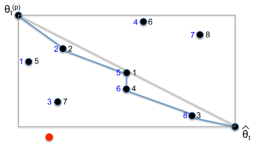
Figure 1: A sketch of the algorithm used to find the path used in the estimator. Points inside of the minimum bounding box between $\theta_{t}^{(p)}$ and $\hat{\theta}_{t}$ are shown in black, and a point outside is shown in red. The points are numbered both in the order of distance to the straight line between $\theta_{t}^{(p)}$ and $\hat{\theta}_{t}$ (in black) from step 2 and in order of the list $\mathcal{L}$ from step 3 (in blue). The resultant path is shown in dark blue.

We will see empirically that, although this approach will not necessarily find the optimal path (except in one dimension, where it yields the path containing all of the points along the line between $\theta_{t}^{(p)}$ and $\hat{\theta}_{t}$), it leads to low variance path estimates.

There are several possible extensions, most notably that if we do not assume that $\mathbb{V}_{\Pi_{i}}\left[S\left(x_{i}\right)\right]$ is constant over $i$, for some models this quantity may be estimated for each $i$ by means of a bootstrap (for example, the block bootstrap for the Ising model) that recycles existing simulations. We note also that since estimates based on different paths are unbiased, we may find estimates based on several different paths and take their mean to combine them and achieve a lower variance.

3 Empirical results

3.1 Ising model

In this section we compare the result of running several different algorithms on a previously studied $10\times 10$ node two-dimensional Ising model. An Ising model is a pairwise Markov random field model on binary variables, each taking values in $\left\{-1,1\right\}$. The data is taken from Friel (2013) and, as in that paper we consider two different neighbourhood structures. In both cases, the variables are arranged in a grid: in the first order model, the neighbours of each node are the nodes horizontally and vertically adjacent to it, with $\mathbf{N}_{1}$ denoting the set of pairs of such neighbours; in the second order model a second set of neighbours are additionally used, with $\mathbf{N}_{2}$ denoting the set of pairs of these neighbours. The distributions of the first and second order models are respectively

$$l_{1}\left(y\mid\theta_{1}\right)\propto\exp\left(\theta_{1}S_{1}\left(y\right)\right),$$

and

$$l_{2}\left(y\mid\theta_{1},\theta_{2}\right)\propto\exp\left(\theta_{1}S_{1}\left(y\right)+\theta_{2}S_{2}\left(y\right)\right),$$

where $\theta_{1},\theta_{2}\in\mathbb{R}$, $y_{i}$ denotes the $i$th random variable in $y$ and $S_{1}\left(y\right)=\sum_{\left(i,j\right)\in\mathbf{N}_{1}}y_{i}y_{j}$, $S_{2}\left(y\right)=\sum_{\left(i,j\right)\in\mathbf{N}_{2}}y_{i}y_{j}$.

We ran the following algorithms 40 times on both models: the exchange algorithm; SAV-MCMC; ABC-MCMC; auxiliary variable marginal SMC (SAV-mSMC) (as in section 2.3.1), and path marginal SMC (path-mSMC) (section 2.3.2) and recorded the estimated posterior expectation and (co)variance in each case. All algorithms were run using $100$ sweeps of a single-site update Gibbs sampler to simulate from the likelihood, taking the final point as the simulated $x$ variable. The same computational budget, measured by the number of simulations from the likelihood which was taken to be $2,000$, was used for each algorithm. For the MCMC algorithms, $2,000$ MCMC iterations were used, with the first $500$ iterations removed as burn in. In ABC-MCMC, the ABC tolerance was chosen to be $\epsilon=0$ in both models, with $S_{1}\left(y\right)$ being the statistic in the first order model and $\left(S_{1}\left(y\right),S_{2}\left(y\right)\right)$ the statistic in the second order model. SAV-MCMC required an estimate $\hat{\theta}$ to construct the SAV estimator. For the first $500$ iterations this was taken to be 0 for the first order model and $\left(0,0\right)$ for the second order model, then for the remaining iterations this was taken to be the sample average of the previous 250 iterations. For the marginal SMC algorithms, 200 particles were used with $T=10$ target distributions. The sequence of target distributions used the annealing scheme described in section 2.2 with $\nu_{t}=\left(t/T\right)^{2}$. The results were compared with the estimated posterior expectation obtained through a long run ($100,000$ iterations with $1,000$ iterations of burn in) of the exchange algorithm, which was taken to be the ground truth. The ground truth is, to 5 s.f, for the first order model $\mathbb{E}_{\pi}\left[\theta_{1}\right]=0.27979$ and for the second order model $\mathbb{E}_{\pi}\left[\theta_{1}\right]=0.36134$ and $\mathbb{E}_{\pi}\left[\theta_{2}\right]=0.080639$.

Algorithm	Exchange	SAV-MCMC	ABC-MCMC	SAV-mSMC	Path mSMC
Bias	$9.68\times 10^{-4}$	$7.96\times 10^{-3}$	$-6.12\times 10^{-2}$	$1.02\times 10^{-5}$	$9.62\times 10^{-4}$
s.d.	$6.35\times 10^{-3}$	$1.32\times 10^{-2}$	$9.21\times 10^{-2}$	$1.11\times 10^{-2}$	$4.81\times 10^{-3}$
RMSE	$6.43\times 10^{-3}$	$1.32\times 10^{-2}$	$1.14\times 10^{-1}$	$1.11\times 10^{-2}$	$4.90\times 10^{-3}$

Table 1: Estimates of bias, standard deviation and root mean square error for estimates of the expectation of $\theta$ in the first order Ising model (rounded to 3 s.f.).

Algorithm	Exchange	SAV-MCMC	ABC-MCMC	SAV-mSMC	Path-mSMC
Bias ($\theta_{1}$)	$4.17\times 10^{-5}$	$-1.41\times 10^{-2}$	$3.42\times 10^{-1}$	$-1.58\times 10^{-3}$	$1.30\times 10^{-3}$
s.d. ($\theta_{1}$)	$1.95\times 10^{-2}$	$3.72\times 10^{-2}$	$5.71\times 10^{-2}$	$4.14\times 10^{-2}$	$1.57\times 10^{-2}$
RMSE ($\theta_{1}$)	$1.95\times 10^{-2}$	$3.98\times 10^{-2}$	$3.47\times 10^{-1}$	$4.14\times 10^{-2}$	$1.57\times 10^{-2}$
Bias ($\theta_{2}$)	$8.00\times 10^{-4}$	$9.18\times 10^{-3}$	$8.68\times 10^{-2}$	$1.57\times 10^{-4}$	$1.24\times 10^{-3}$
s.d. ($\theta_{2}$)	$1.61\times 10^{-2}$	$3.41\times 10^{-2}$	$2.17\times 10^{-2}$	$2.83\times 10^{-2}$	$1.26\times 10^{-2}$
RMSE ($\theta_{2}$)	$1.61\times 10^{-2}$	$3.53\times 10^{-2}$	$8.94\times 10^{-2}$	$2.83\times 10^{-2}$	$1.27\times 10^{-2}$

Table 2: Estimates of bias, standard deviation and root mean square error for estimates of the expectation of $\theta_{1}$ and $\theta_{2}$ in the second order Ising model (rounded to 3 s.f.).

In addition to the methods here, several other algorithms were run. Most notably, we considered a different way of reusing simulations from the likelihood: using regression. In the spirit of papers such as Sherlock et al. (2017), instead of constructing a path estimate using previous samples, we fit a linear regression model with the response being the estimated log-likelihood and the covariates being the values of $\theta$ at which the likelihood was estimated. We found that this was not competitive with other approaches, since a large bias was introduced through the estimate being performed in $\log$-space. We also compared our SMC approach with the method of Koblents and Miguez (2015) which, instead of using an annealed sequence of targets, uses an annealing (or truncation) scheme to regularise the weights of a PMC algorithm, with the annealing changing as the algorithm progresses. We found that the performance of the two approaches is comparable.

Tables 1 and 2 give the bias, standard deviation and root mean square error for estimates of the expectation from the different algorithms. We see that ABC-MCMC exhibits the worst performance: the restriction that the ABC tolerance is zero leads to high variance likelihood estimates, giving an inefficient algorithm. As is emphasised in appendix A, in ABC the use of the simulations from $x$-space is less efficient than for the other methods. SAV-MCMC is outperformed by the exchange algorithm: this is likely due to the fact that the exchange algorithm directly estimates the ratio of partition functions, compared to SAV which uses a ratio of estimates of the reciprocal of partition functions. The results of SAV-mSMC are comparable to SAV-MCMC: there are fewer Monte Carlo points in the SMC approach, but the effective size of the MCMC sample is reduced by the autocorrelation in the chain. Path-mSMC always outperforms SAV-mSMC due to the reduced variance of the likelihood estimates. Figure 2a highlights the improvement of path-mSMC though showing the improved effective sample size (ESS) (Kong et al., 1994) over SAV-mSMC. Figure 2b, which shows the SMC sample over the SMC iterations illustrates why the improvement in ESS is enhanced in the later iterations: the SMC sample concentrates in a small region of the parameter space after around iteration 5, leading to more useful samples being available for the path estimator. Path-mSMC also outperforms the exchange algorithm on this example: in this case the autocorrelation in the sample from the exchange algorithm is outweighed by reduction in variance in the likelihood estimates in path-mSMC.

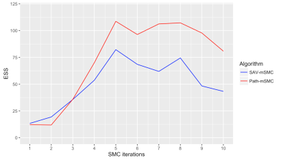
(a) The ESS of the SMC sample at each SMC iteration before resampling for a run of SAV-mSMC and path-mSMC.

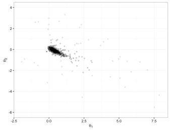
(b) A sequence of samples after resampling from the path-mSMC algorithm applied to the Ising model data. Points from the first annealed target are shown in the lightest grey, with a darker grey for each successive SMC iteration, finishing with black for the final target.

Figure 2: Results from marginal SMC algorithms on the Ising model data.

3.2 Exponential random graph model

Exponential random graph models (ERGMs) are widely used in the analysis of social networks. They describe how distributions over possible networks through weighting the influence of local statistics of the network. The model takes the form

$$f\left(y\mid\theta\right)=\exp\left(\theta^{T}S\left(y\right)\right)/Z\left(\theta\right),$$

with $S\left(y\right)$ being some vector of statistics. Bayesian inference has only relatively recently (Caimo and Friel, 2011) been used for these models, with the exchange algorithm being the most widely used approach, as implemented in the Bergm R package (Caimo and Friel, 2014).

In this section we compare the performance of the exchange algorithm to the new path marginal SMC approach. We study the Dolphin network (Lusseau et al., 2003; Caimo and Friel, 2011), shown in figure 3a, and use the same statistics and priors as in Caimo and Friel (2011). The statistics are

$$S_{1}(y)=\sum_{i<j}y_{ij}$$ the number of edges

$$S_{2}(y)=\exp\left(\phi_{u}\right)\sum_{i=1}^{n-1}\left\{1-\left(1-\exp\left(-\phi_{u}\right)\right)^{i}\right\}D_{i}\left(y\right)$$ geometrically weighted degree

$$S_{3}(y)=\exp\left(\phi_{v}\right)\sum_{i=1}^{n-2}\left\{1-\left(1-\exp\left(-\phi_{v}\right)\right)^{i}\right\}EP_{i}\left(y\right)$$ geometrically weighted edgewise shared partner

and the prior on $\theta$ is $\theta\sim\mathcal{N}(0,30I_{3})$. The ergm package (Hunter et al., 2008) in R was used to simulate from $f\left(\cdot\mid\theta\right)$, which uses the “tie no tie” (TNT) sampler. $15,000$ iterations of the TNT sampler were used, and the $x$ sample was taken to be the final one of these points.

We ran both the exchange algorithm and path-mSMC 40 times, with both algorithms having the same computational budget of $10,000$ simulations from the likelihood. The exchange algorithm was run using the Bergm software. We used two configurations of Bergm: the first using a single chain for $10,000$ iterations with the first $1,000$ iterations discarded as burn in; the second using 6 parallel interacting chains in the same configuration as recommended in Caimo and Friel (2011), with 1667 iterations per chain each with the first $1,000$ iterations discarded as burn in (discarding fewer iterations made relatively insignificant changes to the results). The SMC algorithm was run with $1,000$ particles with $T=10$ SMC targets, again using the annealing scheme with $\nu_{t}=\left(t/T\right)^{2}$. SAV-mSMC did not give useful results for this model, due to the high variance of the estimates of the reciprocal of the partition function. Figure 3b shows the ESS of SAV-mSMC compared to path-mSMC: for many of the iterations the ESS in SAV-mSMC is only marginally above one.

Table 3b gives the bias, standard deviation and root mean square error for estimates of the expectation from the exchange and path-mSMC algorithms, and sequences of samples from path-mSMC are shown in figures 3c, 3d and 3e. As in the previous section, path-mSMC slightly outperforms the exchange algorithm in the main, for the same reasons as in the previous application. For the expectation of $\theta_{2}$ (and also $\theta_{1}$ and $\theta_{3}$ to a lesser degree), the variance of the path-mSMC estimate is increased by one of the 40 runs (without including this run the estimated s.d.s for $\theta_{1}$. $\theta_{2}$ and $\theta_{3}$ respectively are $3.72\times 10^{-2}$, $5.37\times 10^{-2}$ and $1.47\times 10^{-2}$). In this run the ESS was so low in the first iteration that subsequent samples are affected, and the algorithm does not recover. This issue may be rectified by using additional target distributions in between the prior and the first annealed target.

Algorithm	Exchange (single chain)	Exchange (6 chains)	Path-mSMC
s.d. ($\theta_{1}$)	$5.58\times 10^{-2}$	${\color[rgb]{1,0,0}7.33\times 10^{-2}}$	$5.52\times 10^{-2}$
s.d. ($\theta_{2}$)	${\color[rgb]{0,1,0}1.04\times 10^{-1}}$	$1.25\times 10^{-1}$	$4.00\times 10^{-1}$
s.d. ($\theta_{3}$)	$1.97\times 10^{-2}$	$2.65\times 10^{-2}$	${\color[rgb]{0,1,0}1.55\times 10^{-2}}$

Table 3: Estimates of bias, standard deviation and root mean square error for estimates of the expectation of $\theta_{1}$, $\theta_{2}$ and $\theta_{3}$ in the ERGM (rounded to 3 s.f.).

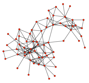
(a) The Dolphin network.

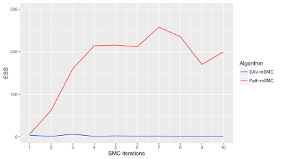
(b) The ESS of the SMC sample at each SMC iteration before resampling for a run of SAV-mSMC and path-mSMC.

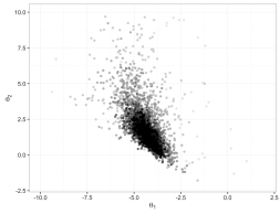
(c) A sequence of samples from the path-mSMC algorithm for $\theta_{1}$ and $\theta_{2}$.

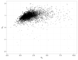
(d) A sequence of samples from the path-mSMC algorithm for $\theta_{2}$ and $\theta_{3}$.

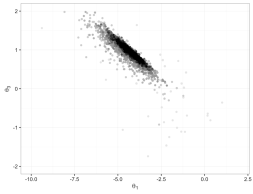
(e) A sequence of samples from the path-mSMC algorithm for $\theta_{1}$ and $\theta_{3}$.

Figure 3: Results from the SMC algorithms applied to the Dolphin network. Where SMC samples are displayed, points from the first annealed target are shown in the lightest grey, with a darker grey for each successive SMC iteration, finishing with black for the final target.

4 Discussion

This paper describes an SMC approach to Bayesian inference of parameters of doubly intractable distributions, through investigating the use of marginal SMC and showing how simulations from earlier iterations of the SMC may be used to reduce the variance of likelihood estimates at future iterations. This offers an alternative to the growing literature on MCMC approaches based on the SAV method and the exchange algorithm (Møller et al., 2006; Murray et al., 2006), and the IS and previous SMC approach in Everitt et al. (2017). Just as in any other situation (outside of the doubly intractable setting), there are cases in which SMC has advantages over MCMC: primarily that with MCMC it can be more difficult to adapt proposal distributions and more difficult to estimate marginal likelihoods. Further, SMC offers a natural way to use a population of Monte Carlo points which may be useful for multi-modal posteriors. In addition, as observed previously in the case of ABC (Sisson et al., 2007), SMC may offer advantages over MCMC in the case where estimated likelihoods are used.

In most settings it is more efficient to use an SMC sampler with MCMC moves compared to the marginal SMC approach (see Didelot et al. (2011) for a practical example of this). However, in the case of doubly intractable distributions we observe two advantages of marginal SMC: firstly there is the flexibility to use any sequence of distributions, where the SMC sampler with MCMC moves is restricted to the case of data point tempered distributions; secondly there is a natural way of reusing previous simulations from the likelihood. We demonstrate good empirical performance for the path-mSMC algorithm, which exploits both of these advantages, and show that without reusing previous simulations the performance of the marginal SMC algorithm may be poor.

Another potential advantage to the approach in this paper is that all of the SMC targets but the final one may be approximate, which may be advantageous if computationally cheap approximate posterior distributions are available. In applications similar to those in this paper, Everitt and Rowińska (2017) make use of approximate targets that use shorter MCMC runs for simulating from the likelihood. We may use such approximations at the early stages of marginal SMC, although it may be difficult to automatically choose which approximation to use at each SMC iteration.

Despite these advantages, there are some limitations to the use of path-mSMC. Most importantly, we expect it to only be effective in low to moderate dimensions: in part due to the use of marginal SMC, and in part due to the reduced effectiveness of the path estimator as the dimension increases.

Appendix A Connecting ABC with the multiple auxiliary variable method

A.1 ABC for doubly intractable models

Suppose that the model $f(y|\theta)$ has an intractable likelihood but can be targeted by a MCMC chain $x=(x_{1},x_{2},\ldots,x_{n})$. Let $\pi$ represent densities relating to this chain. Then $\pi_{n}(y|\theta):=\pi(x_{n}=y|\theta)$ is an approximation of $f(y|\theta)$ which can be estimated by ABC. For now suppose that $y$ is discrete and consider the ABC likelihood estimate requiring an exact match: simulate from $\pi(\mathbf{x}|\theta)$ and return $\mathbbm{1}(x_{n}=y)$. We will consider an IS variation on this: simulate from $g(x|\theta)$ and return $\mathbbm{1}(x_{n}=y)\pi(x|\theta)/g(x|\theta)$. Under the mild assumption that $g(x|\theta)$ has the same support as $\pi(x|\theta)$ (typically true unless $n$ is small), both estimates have the expectation $\Pr(x_{n}=y|\theta)$.

This can be generalised to cover continuous data using the identity

$$\pi_{n}(y|\theta)=\int_{x_{n}=y}\pi(\mathbf{x}|\theta)dx_{1:n-1},$$

where $x_{i:j}$ represents $(x_{i},x_{i+1},\ldots,x_{j})$. An importance sampling estimate of this integral is

$$w=\frac{\pi(\mathbf{x}|\theta)}{g(x_{1:n-1}|\theta)}$$ (12)

where $\mathbf{x}$ is sampled from $g(x_{1:n-1}|\theta)\delta(x_{n}=y)$, with $\delta$ representing a Dirac delta measure. Then, under mild conditions on the support of $g$, $w$ is an unbiased estimate of $\pi_{n}(y|\theta)$.

The ideal choice of $g(x_{1:n-1}|\theta)$ is$\pi(x_{1:n-1}|x_{n},\theta)$, as then $w=\pi(x_{n}=y|\theta)$ exactly. This represents sampling from the Markov chain conditional on its final state being $y$.

A.2 Equivalence to MAV

We now show that natural choices of $\pi(\mathbf{x}|\theta)$ and $g(x_{1:n-1}|\theta)$ in the ABC method just outlined results in the MAV estimator 3. Our choices are

$$g(x_{1:n-1}|\theta) =\prod_{i=1}^{n-1}K_{i}(x_{i}|x_{i+1})$$

$$\pi(\mathbf{x}|\theta) =f_{1}(x_{1}|\theta,y)\prod_{i=1}^{n-1}K_{i}(x_{i+1}|x_{i}).$$

Here $\pi(\mathbf{x}|\theta)$ defines a MCMC chain with transitions $K_{i}(x_{i+1}|x_{i})$. Suppose $K_{i}$ is a reversible Markov kernel with invariant distribution $f_{i}$ for $i\leq a$, and for $i>a$ it is a reversible Markov kernel with invariant distribution $f(\cdot|\theta)$. Also assume $b:=n-a\to\infty$. Then the MCMC chain ends in a long sequence of steps targeting $f(\cdot|\theta)$ so that $\lim_{n\to\infty}\pi_{n}(\cdot|\theta)=f(\cdot|\theta)$. Thus the likelihood being estimated converges on the true likelihood for large $n$. Note this is the case even for fixed $a$.

The importance density $g(x_{1:n-1}|\theta)$ specifies a reverse time MCMC chain starting from $x_{n}=y$ with transitions $K_{i}(x_{i}|x_{i+1})$. Simulating $\mathbf{x}$ is straightforward by sampling $x_{n-1}$, then $x_{n-2}$ and so on. This importance density is an approximation to the ideal choice stated at the end of section A.1.

The resulting likelihood estimator is

$$w=f_{1}(x_{1}|\theta,y)\prod_{i=1}^{n-1}\frac{K_{i}(x_{i+1}|x_{i})}{K_{i}(x_{i}|x_{i+1})}.$$

Using detailed balance gives

$$\frac{K_{i}(x_{i+1}|x_{i})}{K_{i}(x_{i}|x_{i+1})}=\frac{f_{i}(x_{i+1}|\theta,y)}{f_{i}(x_{i}|\theta,y)}=\frac{\gamma_{i}(x_{i+1}|\theta,y)}{\gamma_{i}(x_{i}|\theta,y)},$$

so that

$$w=f_{1}(x_{1}|\theta,y)\prod_{i=1}^{n-1}\frac{\gamma_{i}(x_{i+1}|\theta,y)}{\gamma_{i}(x_{i}|\theta,y)}=\gamma(y|\theta)\prod_{i=2}^{n}\frac{\gamma_{i-1}(x_{i}|\theta,y)}{\gamma_{i}(x_{i}|\theta,y)}.$$

This is an unbiased estimator of $\pi_{n}(y|\theta)$. Hence

$$v=\prod_{i=2}^{n}\frac{\gamma_{i-1}(x_{i}|\theta,y)}{\gamma_{i}(x_{i}|\theta,y)}=\prod_{i=2}^{a}\frac{\gamma_{i-1}(x_{i}|\theta,y)}{\gamma_{i}(x_{i}|\theta,y)}.$$

is an unbiased estimator of $\pi_{n}(y|\theta)/\gamma(y|\theta)\to 1/Z(\theta)$. In the above we have assumed, as in section A.1, that $\gamma_{1}$ is normalised. When this is not the case then we instead get an estimator of $Z(\hat{\theta})/Z(\theta)$, as for MAV methods. Also note that in either case a valid estimator is produced for any choice of $y$.

We note that this carefully designed ABC estimate is precisely the same as the MAV approach. We may view the method as a two stage procedure. First run a MCMC chain of length $b$ with any starting value, targeting $f(\cdot|\theta)$. Let its final value be $x_{a}$. Secondly run a MCMC chain $x_{a},x_{a-1},\ldots$ using kernels $K_{a-1},K_{a-2},\ldots$ and evaluate the estimator $v$. This is unbiased in the limit $b\to\infty$, so the first stage could be replaced by perfect sampling methods where these exist.

A.3 Remark

In this section we have illustrated that a carefully constructed ABC approach (in which the full data is used instead of a summary) yields the same algorithm as the MAV method. We might MAV method to result in an improvement over the standard ABC algorithm due to the more effective use of the simulations from the model $f$. In fact, in section 3 we observe empirically that even the highest variance version of MAV (i.e. the original SAV approach) outperforms ABC in which sufficient statistics are used, i.e. the lowest variance version of ABC.

References

- Aggarwal et al. (2001) Aggarwal, C. C., Hinneburg, A., and Keim, D. A. (2001). On the Surprising Behavior of Distance Metrics in High Dimensional Space. In International Conference on Database Theory, Volume ICDT 2001, pp. 420–434.
- Alquier et al. (2016) Alquier, P., Friel, N., Everitt, R. G., and Boland, A. (2016). Noisy Monte Carlo: Convergence of Markov chains with approximate transition kernels. Statistics and Computing 26(1), 29–47.
- Andrieu and Roberts (2009) Andrieu, C. and Roberts, G. O. (2009). The pseudo-marginal approach for efficient Monte Carlo computations. The Annals of Statistics 37(2), 697–725.
- Beaumont (2003) Beaumont, M. A. (2003). Estimation of population growth or decline in genetically monitored populations. Genetics 164(3), 1139–1160.
- Beaumont et al. (2009) Beaumont, M. A., Cornuet, J.-M., Marin, J.-M., and Robert, C. P. (2009). Adaptive approximate Bayesian computation. Biometrika 96(4), 983–990.
- Bentley (1975) Bentley, J. L. (1975). Multidimensional binary search trees used for associative searching. Communications of the ACM 18(9), 509–517.
- Boland et al. (2017) Boland, A., Friel, N., and Maire, F. (2017). Efficient MCMC for Gibbs Random Fields using pre-computation. arXiv.
- Caimo and Friel (2011) Caimo, A. and Friel, N. (2011). Bayesian inference for exponential random graph models. Social Networks, 33, 41–55.
- Caimo and Friel (2014) Caimo, A. and Friel, N. (2014). Bergm: Bayesian Exponential Random Graphs in R. Journal of Statistical Software 61(2), 1–25.
- Cappé et al. (2004) Cappé, O., Guillin, A., Marin, J.-M., and Robert, C. P. (2004). Population monte carlo. Journal of Computational and Graphical Statistics 13(4), 907–929.
- Chopin et al. (2013) Chopin, N., Jacob, P. E., and Papaspiliopoulos, O. (2013). SMC2: an efficient algorithm for sequential analysis of state space models. Journal of the Royal Statistical Society: Series B 75(3), 397–426.
- Dahlin et al. (2015) Dahlin, J., Lindsten, F., Kronander, J., and Schön, T. B. (2015). Accelerating pseudo-marginal Metropolis-Hastings by correlating auxiliary variables. arXiv, 1–23.
- Del Moral et al. (2006) Del Moral, P., Doucet, A., and Jasra, A. (2006). Sequential Monte Carlo samplers. Journal of the Royal Statistical Society: Series B 68(3), 411–436.
- Del Moral et al. (2012) Del Moral, P., Doucet, A., and Jasra, A. (2012). On adaptive resampling strategies for sequential Monte Carlo methods. Bernoulli 18(1), 252–278.
- Deligiannidis et al. (2016) Deligiannidis, G., Doucet, A., and Pitt, M. K. (2016). The Correlated Pseudo-Marginal Method. arXiv.
- Didelot et al. (2011) Didelot, X., Everitt, R. G., Johansen, A. M., and Lawson, D. J. (2011). Likelihood-free estimation of model evidence. Bayesian Analysis 6(1), 49–76.
- Everitt (2012) Everitt, R. G. (2012). Bayesian Parameter Estimation for Latent Markov Random Fields and Social Networks. Journal of Computational and Graphical Statistics 21(4), 940–960.
- Everitt et al. (2017) Everitt, R. G., Johansen, A. M., Rowing, E., and Evdemon-Hogan, M. (2017). Bayesian model comparison with un-normalised likelihoods. Statistics and Computing 27(2), 403–422.
- Everitt and Rowińska (2017) Everitt, R. G. and Rowińska, P. A. (2017). Delayed acceptance ABC-SMC. arXiv, 1–18.
- Fearnhead et al. (2010) Fearnhead, P., Papaspiliopoulos, O., Roberts, G. O., and Stuart, A. M. (2010). Random-weight particle filtering of continuous time processes. Journal of the Royal Statistical Society Series B 72(4), 497–512.
- Friel (2013) Friel, N. (2013). Evidence and Bayes factor estimation for Gibbs random fields. Journal of Computational and Graphical Statistics 22(3), 518–532.
- Grelaud et al. (2009) Grelaud, A., Robert, C. P., and Marin, J.-M. (2009). ABC likelihood-free methods for model choice in Gibbs random fields. Bayesian Analysis 4(2), 317–336.
- Hunter et al. (2008) Hunter, D. R., Handcock, M. S., Butts, C. T., Goodreau, S. M., and Morris, M. (2008). ergm: A Package to Fit, Simulate and Diagnose Exponential-Family Models for Networks. Journal of Statistical Software 24(3), nihpa54860.
- Klaas et al. (2005) Klaas, M., de Freitas, N., and Doucet, A. (2005). Toward practical Monte Carlo: The marginal particle filter. Proceedings of the 20th International Conference on Uncertainty in Artificial Intelligence.
- Koblents and Miguez (2015) Koblents, E. and Miguez, J. (2015). A population Monte carlo scheme with transformed weights and its application to stochastic kinetic models. Statistics and Computing 25(2), 407–425.
- Kong et al. (1994) Kong, A., Liu, J. S., and Wong, W. H. (1994). Sequential Imputations and Bayesian Missing Data Problems. Journal of the American Statistical Association 89(425), 278–288.
- Liang (2010) Liang, F. (2010, sep). A double Metropolis-Hastings sampler for spatial models with intractable normalizing constants. Journal of Statistical Computation and Simulation 80(9), 1007–1022.
- Liang et al. (2016) Liang, F., Jin, I. H., Song, Q., and Liu, J. S. (2016). An Adaptive Exchange Algorithm for Sampling from Distributions with Intractable Normalizing Constants. Journal of the American Statistical Association 111(513), 377–393.
- Lusseau et al. (2003) Lusseau, D., Schneider, K., Boisseau, O. J., Haase, P., Slooten, E., and Dawson, S. M. (2003). The bottlenose dolphin community of Doubtful Sound features a large proportion of long-lasting associations. Behavioral Ecology and Sociobiology 54(4), 396–405.
- Lyne et al. (2015) Lyne, A.-M., Girolami, M. A., Atchadé, Y. F., Strathmann, H., and Simpson, D. (2015). On Russian Roulette Estimates for Bayesian Inference with Doubly-Intractable Likelihoods. Statistical Science 30(4), 443–467.
- Meeds and Welling (2014) Meeds, E. and Welling, M. (2014). GPS-ABC: Gaussian process surrogate approximate Bayesian computation. Proceedings of the 30th Conference on Uncertainty in Artificial Intelligence.
- Møller et al. (2006) Møller, J., Pettitt, A. N., Reeves, R. W., and Berthelsen, K. K. (2006). An efficient Markov chain Monte Carlo method for distributions with intractable normalising constants. Biometrika 93(2), 451–458.
- Moores et al. (2015) Moores, M. T., Mengersen, K., Drovandi, C. C., and Robert, C. P. (2015). Pre-processing for approximate Bayesian computation in image analysis. Statistics and Computing 25(1), 23–33.
- Murray et al. (2006) Murray, I., Ghahramani, Z., and MacKay, D. J. C. (2006). MCMC for doubly-intractable distributions. In UAI, pp. 359–366.
- Neal (2001) Neal, R. M. (2001). Annealed Importance Sampling. Statistics and Computing 11(2), 125–139.
- Sherlock et al. (2017) Sherlock, C., Golightly, A., and Henderson, D. A. (2017). Adaptive, delayed-acceptance MCMC for targets with expensive likelihoods. Journal of Computational and Graphical Statistics 26(2), 434–444.
- Sisson et al. (2007) Sisson, S. A., Fan, Y., and Tanaka, M. M. (2007). Sequential Monte Carlo without likelihoods. Proceedings of the National Academy of Sciences of the United States of America 104(6), 1760–1765.
- South et al. (2016) South, L. F., Pettitt, A. N., and Drovandi, C. C. (2016). Sequential Monte Carlo for Static Bayesian Models with Independent MCMC Proposals.
- Stoehr et al. (2017) Stoehr, J., Benson, A., and Friel, N. (2017). Noisy Hamiltonian Monte Carlo for Doubly-Intractable Distributions. arXiv, 1–26.
- Wilkinson (2014) Wilkinson, R. D. (2014). Accelerating ABC methods using Gaussian processes. AISTATS, 1015–1023.