A generalised framework for non-classicality of states

Abstract

Non-classical probability (along with its underlying logic) is a defining feature of quantum mechanics. A formulation that incorporates them, inherently and directly, would promise a unified description of seemingly different prescriptions of non-classicality of states that have been proposed so far. This paper sets up such a formalism. It is based on elementary considerations, free of ad-hoc definitions, and is completely operational. It permits a systematic construction of non-classicality conditions on states and also to quantify the non-classicality, at the same time. This quantification, as shown for the example of two level systems, can serve as a measure of coherence and can be furthermore, harnessed to obtain a measure for pure state entanglement for coupled two level systems.

I Introduction

Quantum mechanics has altered the very way we comprehend laws of nature. Equally so, it has altered the way we formulate laws of probability. Thus, the concept of non-classicality of states in quantum physics is as much a reflection of the new probability as it is of non-classical physics. This was recognised quite early, in a rather formal manner, by Birkhoff and von Neumann Birkhoff and Neumann (1936) (see also Jauch and Piron (1969); Accardi (1981)). Recent developments in quantum information, have brought the realization that non-classicality of quantum states can, in fact, act as resources for information processing, some of which could even be impossible otherwiseBennett and Brassard (1984); Bennett et al. (1993). In consequence, many definitions and criteria have been proposed Bell (1964); Clauser et al. (1969); Bell (2004); Kochen and Specker (1967); Werner (1989); Horodecki et al. (1996); Wootters (1998); Collins et al. (2002); Ollivier and Zurek (2001); Wiseman et al. (2007); Alicki et al. (2008); Adhikary et al. (2016). In parallel, there has been a vigorous experimental activity, both for probing the foundations of quantum mechanicsAspect et al. (1981, 1982); Shalm et al. (2015); Giustina et al. (2015) and for eminently practical applicationsBennett and Brassard (1984); Shor (1997); Leach et al. (2009); Ren et al. (2017).

Spectacular though these developments are, our present understanding of non-classicality is not entirely satisfactory. Each definition/criterion is pinned to a specific context, and its interrelationship with other criteria is not always clear. It is, therefore, highly desirable to formulate nonclassicality directly in the language of quantum probabilities and their underlying logic. This would require setting up of a formalism which has (i) non-classical logic (in the sense of Birkhoff and Neumann (1936)) and probability inbuilt in it, (ii) is completely operational and which, in particular, allows for a systematic study of non-classicality conditions. Finally, it should be free of ad-hoc constructions. This task, if accomplished, would provide a unified framework to describe non-classicality of states and allow a systematic way for devising tests for verifying non-classicality of any given state.

This paper sets up such a formalism. Starting from well established, simple, but equally general rules of quantum mechanics, we introduce what we call pseudo projections, and show how they may be harnessed to obtain an infinitely large number of tests of non-classicality of states, within a single framework. This formulation describes non-classicality in a broad setting and hence serves as an encompassing framework. Being operational it also automatically ‘quantifies’ non-classicality. Keeping this operational perspective in mind, we do not wade into the more complicated and unresolved issues concerning the logical foundations of quantum mechanics or of quantum probability, beyond making some essential observations in Section II.5.

After setting up the formalism we illustrate it’s applicability for the simple case of a qubit system. As yet another preliminary application, we show that the quantification of non-classicality through this framework, yields an entanglement monotone for pure two qubit states.

II The Formalism

It is convenient to start with a query, articulated clearly by FineFine (1982a, b): are there circumstances under which a given quantum state permits assignments of joint probabilities for the outcomes of a given set of incompatible observables? This important question, which forms the basis of our analysis, finds its mathematical expression in pseudo-projections.

II.1 Joint probabilities, conjunctions and pseudo-projections

Consider a set of observables, $A^{1},A^{2},\dots,A^{r}$, defined over a phase space ${\Phi}$. Let $A^{k}$ take values belonging to a set $\{a^{k}_{1},a^{k}_{2},\cdots\}$. For a classical system in a state $f$, the joint probability for a conjunction of events $\{A^{1}=a^{1}_{i_{1}},A^{2}=a^{2}_{i_{2}},\cdots,A^{r}=a^{r}_{i_{r}}\}$ always exists and admits a straightforward construction: let $S\subset\Phi$ be the support for the joint outcomes, and $\mathbf{1}_{S}$, its indicator function. Then, the joint probability is given by the overlap of $f$ with $\mathbf{1}_{S}$. By itself, $\mathbf{1}_{S}$ is a Boolean observable: it takes value 1 in $S$ and vanishes outside the support. If $S_{i_{\alpha}}$ are supports for individual outcomes, then $S=\bigcap\limits_{i_{\alpha}}S_{i_{\alpha}}$, which is the set theoretical representation of conjunction.

Observables in quantum mechanics are represented by hermitian operators in a Hilbert space ${\cal H}$. Suppose that $A=\sum_{i}a_{i}\pi_{i}$ is the eigen-resolution of an observable $A$. The eigen-projections $\pi_{i}$ are the quantum representatives of indicator functions; the eigen-projections partition the Hilbert space into a disjoint direct sum of eigenspaces, ${\cal H}=\bigcup\limits_{i}\oplus{\cal H}_{i}$. The subspace ${\cal H}_{i}\equiv\pi_{i}{\cal H}$ is the representative of the corresponding support $S_{i}$. The probability for the outcome $a_{i}$, for a state $\rho$, is given by the overlap, $Tr(\rho\pi_{i})$. Unless the spectrum is continuous, most indicator functions would map to the trivial null projection, of rank zero. The indicator function with the full phase space as its support maps to the identity operator, $\mathbb{1}$.

The crux of the matter is that indicator functions for joint outcomes of observables do not necessarily map to projection operators. This is the statement of uncertainty principle in its primordial form. Nevertheless, we may still inquire into the quantum representatives - hermitian operators - of such indicator functions. This is depicted in Fig. 1 schematically. The quantum representatives will be called pseudo-projections. Pseudo-projections hold the key to non-classicality.

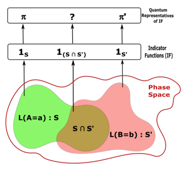
Figure 1: A schematic diagram depicting the indicator functions and their quantum representatives for a pair of events and their conjunction.

II.1.1 Construction of Pseudo-projections

We follow standard rules of quantum mechanics for construction of pseudo-projections. Consider, first, two observables $A,B$. Let $\pi^{A}_{a_{i}},\leavevmode\nobreak\ \pi^{B}_{b_{j}}$ be the projection operators representing the respective indicator functions for the outcomes $A=a_{i}$ and $B=b_{j}$. The unique operator, the pseudo-projection, that represents the indicator function, $\mathbf{1}_{S_{i}\cap S_{j}}$, for the corresponding classical joint outcome, is given by the symmetrised product:

$$\mathbf{\Pi}^{AB}_{a_{i}b_{j}}=\frac{1}{2}\{\pi^{A}_{a_{i}},\pi^{B}_{b_{j}}\},$$ (1)

which is but the simplest example of Weyl ordering Weyl (1927). Though it is hermitian, it is not idempotent and, in fact, admits negative eigenvalues,unless $[\pi^{A}_{a_{i}},\leavevmode\nobreak\ \pi^{B}_{b_{j}}]=0$, i.e., $\mathbf{\Pi}^{AB}_{a_{i}b_{j}}$ is itself a projection. This important property is proved in the appendix. The pseudo projection $\mathbf{\Pi}^{AB}_{a_{i}b_{j}}$ vanishes identically if $\pi^{A}_{a_{i}}=\mathbb{1}-\pi^{B}_{b_{j}}$. This property is consistent with the requirement that the joint probability for an event and its negation should vanish identically .

Pseudo-projections that represent an indicator function for joint outcomes of more than two observables are not unique, reflecting the inherent ambiguity in constructing quantum representatives of classical observables. Symbolically, let ${\Pi}^{N}_{\{\alpha\}}$ be a product of $N$ projections, in some order. The hermitian combination, $\frac{1}{2}(\Pi^{N}_{\{\alpha\}}+\Pi_{\{\alpha\}}^{N\dagger})$, is a legitimate representative of the indicator function for the corresponding joint event. We call this a unit pseudo-projection. For each such classical event there are, in general, $\frac{N!}{2}$ unit projections, which are distinct if no two projection operators commute. Should all the projections corresponding to the $N$ outcomes commute, the manifold of pseudo-projections collapses to a single point and represents a true projection. The convex linear span of distinct unit pseudo-projections yields the family of pseudo-projections that represent the parent indicator function. This fact makes the discussion of joint probability for quantum states richer. Though each choice is equally admissible, and leads to negative eigenvalue(s) in the representative pseudo projections, the one obtained from Weyl ordering, which is the sum of all unit pseudo-projections with equal weights, seems the most favoured: it is completely symmetric in all the projections, as its classical counterpart is, and has a close relationship with Moyal brackets Moyal (1949) and Wigner distribution functions Wigner (1932) which are central to semi classical descriptions.

II.2 Pseudo-projections and pseudo-probabilities

Pseudo-projections generate pseudo-probabilities. Let $\mathbf{\Pi}^{N}(\{A^{\alpha}=a^{\alpha}_{i_{\alpha}}\});\leavevmode\nobreak\ \alpha=1,\cdots,N$, denote the pseudo-projection for the set of the outcomes of $N$ observables indicated in the parenthesis. For a system in a state $\rho$, it generates a pseudo–probability which may be defined as the expectation

$${\cal P}(\{A^{\alpha}=a^{\alpha}_{i_{\alpha}}\})\doteq Tr\Big{[}\rho\mathbf{\Pi}^{N}(\{A^{\alpha}=a^{\alpha}_{i_{\alpha}}\})\Big{]}.$$ (2)

Pseudo-probabilities can take negative values. A complete set of pseudo-probabilities, corresponding to all possible joint outcomes of a given set of observables, is the quantum analogue of the classical joint probability scheme. We call this the pseudo-probability scheme, or in short, the scheme, henceforth. The entries in the schemes do add to unity. The marginal schemes, corresponding to sets of mutually commuting observables, are always true probability schemes, and have entries as mandated by quantum mechanics.

Pseudo-probability schemes serve to define non-classicality of states in an encompassing manner.

II.3 Non-classicality of states

Definition: Let ${\cal S}_{\rho}(\{A^{\alpha}\})$ be the scheme for a set of $N$ observables for a system in a state $\rho$. The state is non-classical with respect to these observables if, even one of the pseudo-probabilities in the scheme is negative. It may be deemed to be classical if, and only if, all the entries are non-negative.

If no restriction is placed on the observables, all states, without exception, turn out to be quantum, as we show in section III.2. However, in importance and as resources, not all states are on equal footing. Therefore, if reasonable restrictions are placed on the choice of observables, or if only certain combinations of pseudo-probabilities are forced, some states would be classical, and others – non-classical. The many prescriptions for designating states as non-classical e.g, Bell (1964); Clauser et al. (1969); Ollivier and Zurek (2001) belong to this category. In short, classicality of a state is relative and not absolute.

Suppose that all the entries in a pseudo-probability scheme are non-negative, even when the underlying projections are mutually non-commuting. It would mean, as it were, that the scheme represents joint probabilities for a correlated classical state, with quantum probabilities as its marginals. Such a scheme automatically yields an explicit construction of contextual hidden parameters for those non-commuting observablesKlyachko et al. (2008). It is important to note that the hidden parameters or, equivalently, the underlying classical systems are not necessarily defined over the same classical phase space that one starts with. This fact becomes clear in our discussion in Section III.

Also, along the sidelines, the definition brings out the real import of the idea of negative probability advocated by Dirac,Dirac (1942), Bartlett Bartlett (1945), and most forcefully, by Feynman Feynman (2012). It has been argued that the introduction of negative probability, even if it be in an ad hoc manner (as in p 11 of Feynman (2012)), does have a role in the sense of consistent book keeping in intermediate processes (and calculations). This intuitive idea, set forth in Dirac (1942); Feynman (2012), gets automatically incorporated in the present formalism. The smallest subset in the event space for which the pseudo-probability is not negative would give the minimum coarse graining required for a physical interpretation of joint probability. For example, for pairs of observables $\sum_{b_{j}}{\cal P}_{a_{i}b_{j}}$ always gives a physically realisable scheme with non-negative entries, but there could be partial sums which yield the same.

II.4 Disjunction and negation

Complete information on non-classicality is captured by schemes, which correspond to the logical conjunction(AND). The quantum representatives of the indicator function corresponding to the two other operations, disjunction (OR) and negation (NOT), may be obtained from their appropriate parent scheme by applying standard probability rules. Thus, the quantum representative of the indicator function representing the disjunction, $A=a_{i}$ OR $B=b_{j}$, which we shall denote ${\bf R}^{AB}_{a_{i}b_{j}}$, has the expression:

$${\bf R}^{AB}_{a_{i}b_{j}} = \sum_{k}{\bf\Pi}^{AB}_{a_{i}b_{k}}+\sum_{k}{\bf\Pi}^{AB}_{a_{k}b_{j}}-{\bf\Pi}^{AB}_{a_{i}b_{j}}$$

$$= \pi^{A}_{a_{i}}+\pi^{B}_{b_{j}}-{\bf\Pi}^{AB}_{a_{i}b_{j}}.$$

In a similar manner, the negation of a pseudo-projection is represented by subtracting it from the identity

$${\bf N}^{AB}_{a_{i}b_{j}}=\mathbb{1}-{\bf\Pi}^{AB}_{a_{i}b_{j}}.$$ (4)

II.5 Differences with classical logic and Kolmogorov formulation

We conclude this section by mentioning briefly how quantum logic (probability) deviates from the classical (Kolmogorov) formulation. First of all, consider pseudo projections. Non-classical logic, as understood in Birkhoff and Neumann (1936), is inherent in the very definition of pseudo projections. The formalism developed in Birkhoff and Neumann (1936) identifies joint outcomes of non-commuting observables with absurd propositions in the quantum domain, although they are perfectly valid classically. The violations of Boolean logic that they aver arise from this identification. The present work does capture this qualitative observation more sharply and quantitatively, through the emergence of negative eigenvalue(s) of the corresponding pseudo-projections.

Pseudo probability schemes capture non-classical probability by violating the very first Kolmogorov axiom for probability theory which states that the probability for any event $E$, $P(E)\in\mathbb{R};\leavevmode\nobreak\ P(E)\geq 0$. Some random variables can be assigned negative probabilities and, consequently, there will be other random variables for which the assignment of probabilities would exceed one (this can be seen, e.g., in the case of negation). The other two axioms are preserved.

Quantum mechanics is distinguished from other theories which employ negative probability Popescu and Rohrlich (1994) by virtue of the fact that the number of negative probabilities is controlled strictly by the spectrum of pseudo projections.

We devote the rest of the paper to illustrate the salient features of non-classicality for two level systems, with a very brief mention of pure state entanglement. Only mutually non-commuting projections will be used in construction of pseudo projections, henceforth.

III Non-classicality in two level systems

The phase space underlying a two level system is compact, and is endowed with the Poisson bracket
$\{\vec{S}\cdot\hat{m},\vec{S}\cdot\hat{n}\}\ =\vec{S}\cdot(\hat{m}\times\hat{n})$. The quantum mechanical states have the form $\rho=\frac{1}{2}(\mathbb{1}+\vec{\sigma}\cdot\vec{P});|\vec{P}|\leq 1$. Observables have the form $A_{i}=\vec{\sigma}\cdot\vec{m}_{i}$, apart from the trivial identity. The two eigen-projections belonging to the respective eigenvalues $\pm|\vec{m}|$ of $A$ are given by $\pi_{a}=\frac{1}{2}(1+a\vec{\sigma}\cdot\hat{m})$; $a=\pm 1$.

The set {$\pi_{a}$} exhausts all possible projections and, hence, outcomes of all possible measurements involving single observables. Thus, classically - in the sense of probability – it should be possible to assign joint probabilities for possible values $\{\pm 1\}^{N}$ with respect to sets of directions {$\hat{m_{i}}\};\leavevmode\nobreak\ i=1,2,\cdots N$, with the proviso that for each of them,

$$P_{c}\Big{(}A(\hat{m})=1\Big{)}=p_{1}\implies P_{c}\Big{(}A(-\hat{m})=1\Big{)}=1-p_{1}.$$ (5)

A complete probability scheme would then consist of assigning joint probabilities for all points on a unit sphere (see Eq.(5)), which would but be very highly correlated. If such a scheme exists for a given quantum mechanical state, the underlying classical space would be quite distinct from the phase space for the two level system which we started with. A correspondence between the two spaces exists only when $N\leq 3$ and the directions are mutually orthogonal.

Quantum mechanics forbids the existence of such probability assignments, even when $N=2$. This gets reflected in the emergence of negative entries in the corresponding schemes.

III.1 Non-classicality with respect to pairs of observables

Let $A_{1},A_{2}$ be two observables, each having two outcomes: $a_{1,2}=\pm 1$. The corresponding complete set of pseudo-projections for their joint occurrence is given, in terms of respective projections, by

$$\mathbf{\Pi}_{a_{1}a_{2}}=\frac{1}{2}\{\pi_{a_{1}},\pi_{a_{2}}\};\leavevmode\nobreak\ a_{1,2}=\pm 1.$$ (6)

The four pseudo-probabilities for a qubit in a state $\rho$ can be read off as

$${\cal P}_{a_{1}a_{2}}=\frac{1}{4}\Big{\{}1+a_{1}a_{2}\hat{m}_{1}\cdot\hat{m}_{2}+\vec{P}\cdot(a_{1}\hat{m}_{1}+a_{2}\hat{m}_{2})\Big{\}}.$$ (7)

As mentioned, the marginal scheme obtained by summing over $a_{1}$ yields the quantum mechanical probabilities for $A_{2}$ and vice versa.

Several quick conclusions may be drawn from Eq.(7). It follows from Eq.(7) that at most one entry in the pseudo probability scheme can be negative, while, the requirement of proper marginals would allow for two negative values. This feature is characteristic of quantum mechanics, distinguishing it from other physical theories/models Popescu and Rohrlich (1994).

Significantly, if no condition on the two directions is imposed, all states, except the completely mixed state, turn out to be non-classical. More explicitly, so long as $|\vec{P}|\neq 0$, one can always find two observables for which the scheme becomes negative. Let us, therefore, impose the restriction $\hat{m}_{1}\cdot\hat{m}_{2}=0$, which is equivalent to simultaneous specification of two orthogonal components of the classical spin vector. With this restriction, the condition on classicality gets diluted. Indeed, a state would be deemed to be classical so long as $|\vec{P}|\leq\frac{1}{\sqrt{2}}$, covering about 70% of the volume of the state space. This conclusion, together with extension to three orthogonal observables, is dual to the POVM for joint measurement of observablesBusch (1986).

Remarkably, Eq.(7) coincides with the expression obtained by Cohen and Scully Cohen and Scully (1986) who, starting with quantum analog of characteristic functions for a pair of observables in a two level system, computed the probability for their joint outcomes. This exact agreement merits further investigation. More pertinently, the present work, apart from being much simpler, clarifies the precise meaning of what Cohen and Scully Cohen and Scully (1986) mean by joint probability, and goes beyond, by developing a general framework with applicability to any number of observables.

III.2 Non-classicality with respect to triplets of observables

Let ${\bf\Pi}_{ab}$ be a pseudo-projection. It has an important physical interpretation. It represents conditional probabilities which are inherent to quantum mechanics. For, if a system is in a state $\rho_{a}=\pi_{a}$, then $Tr(\rho_{a}\mathbf{\Pi}_{ab})\equiv P(b|a)=P(a|b)$ is but the Born rule for the probability that the outcome of a measurement of $B$ yields a value $b$, and vice versa. Von Neumann observes that the symmetry in the Born rule is a defining feature of quantum mechanics Neumann (1955).

A similar requirement on classical conditional probability would force the equality Accardi (1981)

$$P_{c}(a|b)\doteq\frac{P_{c}(a,b)}{P_{c}(b)}=P_{c}(b|a)\doteq\frac{P_{c}(a,b)}{P_{c}(a)}$$ (8)

which holds if, and only if, both $P_{c}(a)$ and $P_{c}(b)$ are uniform distributions, and thus, $P_{c}(a,b)$ is itself uniform. This result is in consonance with our finding that no joint probability description exists for two observables, unless the state is completely mixed. Is it possible that the uniform distributions also may retain non-classical features, not revealed by pairs of observables? To answer this, we consider sets of three observables.

Let $A_{1}$, $A_{2}$ and $A_{3}$ be three observables, $A_{i}=\vec{\sigma}\cdot\hat{m}_{i}$. The corresponding pseudo projections, and hence, the resultant pseudo-probability scheme is, however, not unique. Associated with any given joint outcome $\{a_{1},a_{2},a_{3}\}$, of the three observables, there are three distinct inequivalent unit-pseudo-projections (the projections are mutually non-commuting),

$${\bf\Pi}^{(1)}_{a_{1}a_{2}a_{3}}=\frac{1}{2}(\pi_{a_{1}}\pi_{a_{2}}\pi_{a_{3}}+\pi_{a_{3}}\pi_{a_{2}}\pi_{a_{1}})$$

$${\bf\Pi}^{(2)}_{a_{1}a_{2}a_{3}}=\frac{1}{2}(\pi_{a_{3}}\pi_{a_{1}}\pi_{a_{2}}+\pi_{a_{2}}\pi_{a_{1}}\pi_{a_{3}})$$

$${\bf\Pi}^{(3)}_{a_{1}a_{2}a_{3}}=\frac{1}{2}(\pi_{a_{2}}\pi_{a_{3}}\pi_{a_{1}}+\pi_{a_{1}}\pi_{a_{3}}\pi_{a_{2}})$$ (9)

One can form further convex combinations of the three unit pseudo projections. Each combination is a legitimate representative of the parent indicator function. All these constructions are mutually inequivalent.

Be it as it may, inequivalent pseudo projections can still exhibit a broad class-equivalence when their action on the full state space is considered. They may exhibit the same universal features. As an example, we may note that the three unit pseudo projections, being related to each other by permutations, possess this broad equivalence. This extends to other classes also provided the members are related to each other by permutation symmetry.

Of all the representatives, the completely symmetric pseudo projection, obtained by Weyl ordering is of special interest (see II.1.1). We focus our attention to the scheme obtained by Weyl ordering. The associated pseudo probabilities have the form

$${\cal P}_{a_{1}a_{2}a_{3}} = \frac{1}{8}\Big{(}1+\vec{P}\cdot\sum_{i=1}^{3}a_{i}\hat{m}_{i}+\sum_{i<j=1}^{3}a_{i}a_{j}\hat{m}_{i}\cdot\hat{m}_{j}$$ (10)

$$+ \frac{1}{3}a_{1}a_{2}a_{3}\sum_{(ijk)}\vec{P}\cdot\hat{m}_{i}\hat{m}_{j}\cdot\hat{m}_{k}\Big{)}$$

where ($i,j,k$) are distinct and vary cyclically in the last term; $a_{i}=\pm 1$.

Eq. (10) answers the question raised at the beginning of this section. Even the completely mixed state is not immune to non-classical behaviour. To see this, consider the symmetric coplanar geometry of the three directions given by $\hat{m}_{i}\cdot\hat{m_{j}}=-\frac{1}{2};i\neq j$, and construct the scheme for the completely mixed state ($|\vec{P}|=0$). We get, two negative pseudo probabilities ${\cal P}_{111}={\cal P}_{-1-1-1}=-\frac{1}{16}$, with the other six pseudo probabilities being positive and having equal values, dashing any hope that the completely mixed state is classical with respect to any set of observables.

We conclude the section by revisiting the restriction that the three observables be mutually orthogonal. For this case, which has received much attention in the context of POVM, the assignments of values $\pm 1$ is perfectly consistent with the classical requirement. The corresponding scheme is, however, non-negative only if $|\vec{P}|\leq\frac{1}{\sqrt{3}}$. This renders about 58% of the volume classical.

IV Quantitative features of non-classicality

We now examine more quantitative features of non-classicality that emerge from pseudo projections. We begin by designing a suitable measure for non-classicality of a state. We call this measure, negativity, and define it as

$$\mathcal{N}=\frac{1}{2}(\sum_{i}|\mathcal{P}_{i}|-1)$$ (11)

where the summation runs over all entries in the pseudo-probability scheme. A state is non-classical, with respect to a set of observables, if $\mathcal{N}>0$. For any given state, ${\cal N}$ is a monotonically increasing function of purity, though not necessarily strictly. Of greater interest is the relative volume of the state space that is rendered non-classical by a family of observables. As a concrete example we consider the set of all pairs of observables, $\{\vec{\sigma}\cdot\hat{m}_{1},\vec{\sigma}\cdot\hat{m}_{2}\}$. Then negativity is given, for the special geometry $\vec{P}\parallel\hat{m}_{1}+\hat{m}_{2}$ by

$$\mathcal{N}=\frac{1}{2}\Big{(}|\vec{P}|\cos\frac{\theta}{2}-\cos^{2}\frac{\theta}{2}\Big{)}.$$ (12)

Here $\hat{m}_{1}\cdot\hat{m}_{2}=\cos\theta$. It follows that the state is non classical only so long as $|\vec{P}|>\cos\frac{\theta}{2}$. The full behaviour of negativity is shown in Fig. 2 for two values of polarisation. More conclusions can be drawn from this figure:

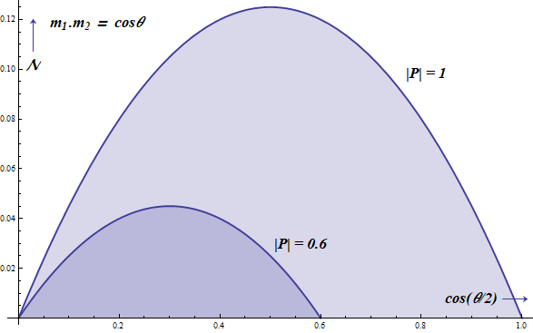
Figure 2: Variation of negativity $\mathcal{N}$ with the geometry of the observables for different values of purity.

1. For a fixed value of $\theta$, ${\cal N}$ is a strictly increasing function of purity. Thus, it can act as a measure of coherence as well.

2. The maximum value of ${\cal N}$ is also a strictly increasing monotonic function of purity; ${\cal N}_{max}=\frac{|\vec{P}|^{2}}{8}$.

3. The region of the parameter space (the relative volume in the space of observables) over which negativity is non-zero, shrinks as the mixedness of the state increases. For example for the completely mixed state $\mathcal{N}$ is zero for all possible combinations of observables whereas, for the pure state negativity is non-zero over the entire range of $\theta\in(0,\pi)$.

IV.1 Negativity as a pure state entanglement monotone

Finally, we round up the discussion with an application to quantify pure state entanglement in two qubit states. The degree of entanglement in a pure two qubit state is uniquely determined by the mixedness of it’s reduced density matrix. Negativity, being a monotonic function of purity (of the reduced density matrices), can therefore be construed as a useful entanglement monotone for pure two qubit states. For instance, the quantity $\mathcal{M}=1-\{\mathcal{N}_{max}(\rho_{r})/\mathcal{N}_{max}(\rho_{p})\}$ serves as a valid measure of entanglement for a pure two qubit state $|\psi\big{>}$; here $\rho_{r}$ is the reduced density matrix of $|\psi\big{>}$ while $\rho_{p}$ is a pure state belonging to the same subsystem and $\mathcal{N}_{max}$ is calculated form Eq.(12). $\mathcal{M}$ goes to zero when $|\psi\big{>}$ is factorizable and to unity when the state is maximally entangled. It is easy to construct similar quantities from pseudo-probability schemes involving larger number of observables. Nevertheless the case involving just a pair of observables continues to remain the simplest. Though this observation may appear to be rather simplistic, we show in the next paper that a judicious combination of logical propositions and combinations of pseudo probabilities permit construction of a series of witnesses for entanglement in two qubit states.

V Conclusion

In summary, quantum probabilities and their underlying logic find their natural formulation through our framework, in the language of pseudo-projections and pseudo-probabilities. This framework is completely operational and allows for a comprehensive description of non-classicality. This opens up a fertile field where non-classicality may be studied in all its avatars. In this paper we have focussed on application to two level systems and have developed a quantitative measure of non-classicality that can be used as a measure of coherence. We have further shown how this measure can be harnessed to infer the amount of entanglement in a pure two qubit state. Many interesting results follow when we extend our work to multiparty systems as well as to higher dimensional systems. These will be reported in subsequent publications.

Appendix A Pseudo projections have at least one negative eigenvalue

We show, in this appendix, that pseudo projections in any dimension $D$, and with any number of incompatible observables $N$, have, at least, one negative eigenvalue. Consider, first, two incompatible projections in $D=2$. The pseudo projection

$${\bf\Pi}^{\hat{m}_{1}\hat{m}_{2}}_{a_{1}a_{2}}=\frac{1}{2}\{\pi^{m_{1}}_{a_{1}},\pi^{m_{2}}_{a_{2}}\}$$ (13)

has exactly one negative eigenvalue. If we now increase the number of observables, since ${\bf\Pi}^{\hat{m}_{1}\hat{m}_{2}}_{a_{1}a_{2}}$ is the marginal of the complete set of the corresponding pseudo projections, it follows that the result is valid for any value of $N$ as well. We extend the result to $D\geq 3$, by induction. Indeed, a pseudo projection defined in $D\geq 3$ yields a pseudo projection in $D=2$ on taking its projection to the appropriate two dimensional subspace, thereby leading to a contradiction if the spectrum of the parent pseudo projection were to be non negative.

References

- Birkhoff and Neumann (1936) G. Birkhoff and J. V. Neumann, Annals of Mathematics 37, 823 (1936).
- Jauch and Piron (1969) J. M. Jauch and C. Piron, Helvetica Physica Acta 42, 842 (1969).
- Accardi (1981) L. Accardi, Physics Reports 77, 169 (1981).
- Bennett and Brassard (1984) C. Bennett and G. Brassard, Proc. IEEE Int. Conf. on Comp. Sys. Signal Process (ICCSSP) , 175 (1984).
- Bennett et al. (1993) C. H. Bennett, G. Brassard, C. Crépeau, R. Jozsa, A. Peres, and W. K. Wootters, Phys. Rev. Lett. 70, 1895 (1993).
- Bell (1964) J. S. Bell, Physics 1, 195 (1964).
- Clauser et al. (1969) J. F. Clauser, M. A. Horne, A. Shimony, and R. A. Holt, Phys. Rev. Lett. 23, 880 (October 1969).
- Bell (2004) J. S. Bell, Speakable and Unspeakable in Quantum Mechanics: Collected Papers on Quantum Philosophy (Cambridge University Press, 2004).
- Kochen and Specker (1967) S. Kochen and E. P. Specker, Journal of mathematics and mechanics 17, 59 (1967).
- Werner (1989) R. F. Werner, Physical Review A 40, 4277 (1989).
- Horodecki et al. (1996) R. Horodecki, P. Horodecki, and M. Horodecki, Physics Letters A 210, 377 (1996).
- Wootters (1998) W. K. Wootters, Phys. Rev. Lett. 80, 2245 (1998).
- Collins et al. (2002) D. Collins, N. Gisin, N. Linden, S. Massar, and S. Popescu, Phys. Rev. Lett. 88, 040404 (2002).
- Ollivier and Zurek (2001) H. Ollivier and W. H. Zurek, Phys. Rev. Lett. 88, 017901 (2001).
- Wiseman et al. (2007) H. M. Wiseman, S. J. Jones, and A. C. Doherty, Phys. Rev. Lett. 98, 140402 (2007).
- Alicki et al. (2008) R. Alicki, M. Piani, and N. V. Ryn, Journal of Physics A: Mathematical and Theoretical 41, 495303 (2008).
- Adhikary et al. (2016) S. Adhikary, I. K. Panda, and V. Ravishankar, Annals of Physics , (2016).
- Aspect et al. (1981) A. Aspect, P. Grangier, and G. Roger, Phys. Rev. Lett. 47, 460 (1981).
- Aspect et al. (1982) A. Aspect, P. Grangier, and G. Roger, Phys. Rev. Lett. 49, 91 (1982).
- Shalm et al. (2015) L. K. Shalm, E. Meyer-Scott, B. G. Christensen, P. Bierhorst, M. A. Wayne, M. J. Stevens, T. Gerrits, S. Glancy, D. R. Hamel, M. S. Allman, K. J. Coakley, S. D. Dyer, C. Hodge, A. E. Lita, V. B. Verma, C. Lambrocco, E. Tortorici, A. L. Migdall, Y. Zhang, D. R. Kumor, W. H. Farr, F. Marsili, M. D. Shaw, J. A. Stern, C. Abellán, W. Amaya, V. Pruneri, T. Jennewein, M. W. Mitchell, P. G. Kwiat, J. C. Bienfang, R. P. Mirin, E. Knill, and S. W. Nam, Phys. Rev. Lett. 115, 250402 (2015).
- Giustina et al. (2015) M. Giustina, M. A. M. Versteegh, S. Wengerowsky, J. Handsteiner, A. Hochrainer, K. Phelan, F. Steinlechner, J. Kofler, J.-A. Larsson, C. Abellán, W. Amaya, V. Pruneri, M. W. Mitchell, J. Beyer, T. Gerrits, A. E. Lita, L. K. Shalm, S. W. Nam, T. Scheidl, R. Ursin, B. Wittmann, and A. Zeilinger, Phys. Rev. Lett. 115, 250401 (2015).
- Shor (1997) P. Shor, SIAM Journal on Computing 26, 1484 (1997).
- Leach et al. (2009) J. Leach, B. Jack, J. Romero, M. Ritsch-Marte, R. Boyd, A. Jha, S. Barnett, S. Franke-Arnold, and M. J. Padgett, Opt. Express 17, 8287 (2009).
- Ren et al. (2017) J.-G. Ren, P. Xu, H.-L. Yong, L. Zhang, S.-K. Liao, J. Yin, W.-Y. Liu, W.-Q. Cai, M. Yang, L. Li, et al., Nature 549, 70 (2017).
- Fine (1982a) A. Fine, Phys. Rev. Lett. 48, 291 (1982a).
- Fine (1982b) A. Fine, Journal of Mathematical Physics 23, 1306 (1982b).
- Weyl (1927) H. Weyl, Zeitschrift für Physik 46, 1 (1927).
- Note (1) More sophisticated ramifications involving multiple observables will be discussed separately.
- Moyal (1949) J. E. Moyal, Mathematical Proceedings of the Cambridge Philosophical Society 45, 99–124 (1949).
- Wigner (1932) E. Wigner, Phys. Rev. 40, 749 (1932).
- Klyachko et al. (2008) A. A. Klyachko, M. A. Can, S. Binicioğlu, and A. S. Shumovsky, Phys. Rev. Lett. 101, 020403 (2008).
- Dirac (1942) P. A. M. Dirac, Proceedings of the Royal Society of London A: Mathematical, Physical and Engineering Sciences 180, 1 (1942).
- Bartlett (1945) M. S. Bartlett, Mathematical Proceedings of the Cambridge Philosophical Society 41, 71–73 (1945).
- Feynman (2012) R. P. Feynman, Chapter- 13, Quantum implications: essays in honour of David Bohm (edited by B. Hiley and F. Peat) (Taylor & Francis, 2012) pp. 235–248.
- Note (2) This formal definition, however, fails to obey the fundamental classical rule that would require .
- Popescu and Rohrlich (1994) S. Popescu and D. Rohrlich, Foundations of Physics 24, 379 (1994).
- Busch (1986) P. Busch, Phys. Rev. D 33, 2253 (1986).
- Cohen and Scully (1986) L. Cohen and M. O. Scully, Foundations of Physics 16, 295 (1986).
- Neumann (1955) J. V. Neumann, Mathematical foundations of quantum mechanics (Princeton University Press, 1955).