On the local stability of semidefinite relaxations

Abstract.

We consider a parametric family of quadratically constrained quadratic programs (QCQP) and their associated semidefinite programming (SDP) relaxations. Given a nominal value of the parameter at which the SDP relaxation is exact, we study conditions (and quantitative bounds) under which the relaxation will continue to be exact as the parameter moves in a neighborhood around the nominal value. Our framework captures a wide array of statistical estimation problems including tensor principal component analysis, rotation synchronization, orthogonal Procrustes, camera triangulation and resectioning, essential matrix estimation, system identification, and approximate GCD. Our results can also be used to analyze the stability of SOS relaxations of general polynomial optimization problems.

1. Introduction

A number of parameter estimation problems [1, 37, 19, 33, 30, 10, 11, 40, 24, 9, 36, 5, 27] in statistics and engineering can be posed as minimizing a polynomial over an algebraic variety. For example, a commonly occurring form is:

(1) $$\min_{y,z}\ \|y-\theta\|^{2},\qquad\text{s.t.}\qquad g(y,z)=0.$$

where $\theta$ is a vector of noisy observations from the model which is an algebraic variety described by a system of quadratic polynomials $g$. The aim is to find $y$ and $z$ that best explains the observations $\theta$, and by best we mean the maximum likelihood estimate (MLE) of $y$ and $z$. Problem (1) is an instance of a quadratically constrained quadratic program (QCQP). While QCQPs are hard to solve, their Lagrangian duals are semidefinite programs (SDP) that can be solved efficiently. In general this SDP is a relaxation of the QCQP in the sense that its optimal value is only a lower bound to the optimal value of the QCQP. However, in some instances, their values agree (i.e. the duality gap is zero) and we say that the SDP relaxation is tight. Indeed this has been found to happen in a number of estimation problems in practice, when the noise is small. We illustrate this phenomenon on the following simple example:

Example 1.1 (Nearest point to the twisted cubic).

Let $\mathbf{Y}:=\{(t,t^{2},t^{3}):t\in{\mathbb{R}}\}$ be the twisted cubic curve in ${\mathbb{R}}^{3}$. Consider the problem of finding the nearest point from $\theta\in{\mathbb{R}}^{3}$ to the curve $\mathbf{Y}$. This problem can be phrased as the QCQP:

(2) $$\min_{y\in\mathbf{Y}}\quad \|y-\theta\|^{2},\quad\text{ where }\quad\mathbf{Y}=\{y\in{\mathbb{R}}^{3}:y_{2}\!=\!y_{1}^{2},\;y_{3}\!=\!y_{1}y_{2}\}.$$

Its Lagrangian dual is the SDP:

(3) $$\max_{\lambda_{0},\lambda_{1},\lambda_{2}\in{\mathbb{R}}} -\lambda_{0},\quad\text{s.t.}\quad\left(\begin{smallmatrix}\lambda_{0}+\|\theta\|^{2}&-\theta_{1}&\lambda_{1}-\theta_{2}&\lambda_{2}-\theta_{3}\\ -\theta_{1}&1-2\lambda_{1}&-\lambda_{2}&0\\ \lambda_{1}-\theta_{2}&-\lambda_{2}&1&0\\ \lambda_{2}-\theta_{3}&0&0&1\end{smallmatrix}\right)\succeq 0.$$

Figure 1 shows the projection of $Y$ onto the $y_{1}y_{3}$-plane, and the duality gap for parameters $\theta$ of the form $(\theta_{1},\theta_{1}^{2},\theta_{3})$. For all parameters in the dotted region around $\mathbf{Y}$, the QCQP has zero-duality gap in the sense that its optimal value agrees with that of its Lagrangian dual.

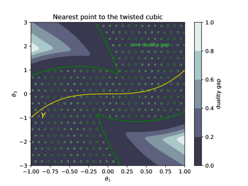
Figure 1. Duality gap in the QCQP (2) for parameters $\theta$ of the form $(\theta_{1},\theta_{1}^{2},\theta_{3})$. There is no duality gap in the dotted region.

Problem (1) has the property that if $\theta$ is noiseless, i.e., $\theta=\bar{\theta}$ lies on the algebraic variety, then the QCQP corresponding to $\bar{\theta}$ has zero duality gap. The interesting feature is that in many instances, as in the above example, (1) continues to have zero duality gap when $\theta$ is close to $\bar{\theta}$. In some cases, there are problem specific explanations for when we can expect the relaxation to be tight under low noise [1, 33, 37, 19]. There is, however, no general understanding of this phenomenon. The aim of this paper is to fill this gap.

One approach to studying the tightness of SDP relaxations in the low noise regime is to think of problem (1) as a perturbation of a noiseless instance, whose relaxation is tight. This is the perspective we will take in this paper. Further, we will not limit ourselves to the special problem in (1) and will instead consider general QCQPs.

We point out that our focus on SDP relaxations from QCQPs does not pose a practical limitation, since most of the SDP relaxations used in practice arise in such a way. In some cases, though, the QCQP is not immediately apparent to the user. For instance, the nuclear norm minimization problem $\min\{\|M\|_{*}:M\!\in\!{\mathbb{R}}^{m\times n},\mathcal{A}(M)\!=\!b\}$, which can be rewritten as an SDP, and is often used [16] to find a low rank matrix $M$ satisfying affine constraints $\mathcal{A}(M)\!=\!b$, arises as the relaxation of the QCQP $\min\{\frac{1}{2}(\|u\|^{2}\!+\!\|v\|^{2}):u\!\in\!{\mathbb{R}}^{m},v\!\in\!{\mathbb{R}}^{n},\mathcal{A}(uv^{T})\!=\!b\}$.

The problem we consider is the following. Let $\Theta\subseteq{\mathbb{R}}^{d}$ be a parameter space, and consider a family of QCQPs parametrized by $\theta\in\Theta$:

(Q) $$\min_{x\in{\mathbb{R}}^{N}} f_{\theta}(x):=x^{\top}F_{\theta}x$$

s.t. $$g_{\theta}^{i}(x):=x^{\top}G_{\theta}^{i}x+c^{i}_{\theta}=0,\quad i=1,\dots,m$$

where $F_{\theta},G^{i}_{\theta}\in{\mathbb{S}}^{N}$ are symmetric $N\times N$ matrices, and $c^{i}_{\theta}\in{\mathbb{R}}$ are scalars. We assume that at least one $c^{i}_{\theta}$ is nonzero, which ensures that $x\!=\!0$ is not a solution of (Q). We will also assume that the map $\theta\mapsto(F_{\theta},G^{i}_{\theta},c^{i}_{\theta})$ is continuous. A QCQP such as (Q) that involves no linear terms is said to be homogeneous. While our main results are formulated for homogeneous QCQPs, in each case we also write down the accompanying statement for the inhomogeneous version.

The QCQP (Q) has an associated pair of SDP relaxations that are dual to each other:

(P) $$\min_{S\in{\mathbb{S}}^{N}} {F_{\theta}}\bullet S$$

s.t. $$G^{i}_{\theta}\bullet S+c^{i}_{\theta}=0,\quad i=1,\dots,m$$

$$S\succeq 0$$

(D) $$\max_{\lambda\in{\mathbb{R}}^{m}} \textstyle\sum_{i}\lambda_{i}c^{i}_{\theta}$$

s.t. $$\mathcal{H}_{\theta}(\lambda):=F_{\theta}+\textstyle\sum_{i}\lambda_{i}G^{i}_{\theta}\succeq 0$$

where $\bullet$ denotes the trace inner product in ${\mathbb{S}}^{N}$. The SDP (P) will be referred to as the primal SDP relaxation of (Q). There is a bijection between the solutions of (Q) and the rank one solutions of (P) via $x\mapsto xx^{\top}$. Hence, if an optimal solution of (P) has rank one, then (P) recovers a minimizer of (Q). Problem (P) is sometimes known as the Shor relaxation of (Q).

Problem (D) is the dual SDP of (P) as well as the Lagrangian dual of (Q). Its objective function is traditionally written as $\max_{\lambda\in{\mathbb{R}}^{m}}\min_{x\in{\mathbb{R}}^{N}}L_{\theta}(x,\lambda)$ where

$$L_{\theta}(x,\lambda)=f_{\theta}(x)+\sum_{i}\lambda_{i}g^{i}_{\theta}(x)$$

is the Lagrangian function of (Q). Note that $\mathcal{H}_{\theta}(\lambda)=\tfrac{1}{2}\,\nabla^{2}_{xx}L_{\theta}(x,\lambda)$ is half the Hessian of the Lagrangian.

The inequalities $\operatorname{val}{\eqref{eq:Qtheta}}\geq\operatorname{val}{\eqref{eq:Ptheta}}\geq\operatorname{val}{\eqref{eq:Dtheta}}$ always hold. We say that (Q) has zero duality gap if $\operatorname{val}{\eqref{eq:Qtheta}}=\operatorname{val}{\eqref{eq:Ptheta}}=\operatorname{val}{\eqref{eq:Dtheta}}$. Throughout this paper we denote by $\bar{\theta}$ a nominal value of the parameter $\theta$, such that ($Q_{\bar{\theta}}$) has zero duality gap.

Definition 1.2 (SDP Stability).

The family ${\eqref{eq:Qtheta}}$ is SDP-stable near $\bar{\theta}$ if there exists a neighborhood of $\bar{\theta}$ where $\operatorname{val}{\eqref{eq:Qtheta}}=\operatorname{val}{\eqref{eq:Ptheta}}=\operatorname{val}{\eqref{eq:Dtheta}}$.

In this paper we will derive theorems that establish SDP-stability of (Q) near $\bar{\theta}$, so that the optimal value of the SDP relaxation agrees with that of the QCQP when $\theta$ is close to $\bar{\theta}$. Moreover, the conditions in our theorems also guarantee that the SDP relaxation (P) recovers the minimizer of the QCQP.

Contributions and structure of the paper

We start this paper, in Section 2, by recalling a simple sufficient condition for zero duality gap in QCQPs. As a corollary, the SDP relaxation of the nearest point problem to a quadratic variety is tight, when the observed point is on the variety.

Our main contribution consists of two stability results that guarantee zero duality gap for (Q) when $\theta$ close to $\bar{\theta}$. Our first result is Theorem 3.2 in Section 3 which focuses on QCQPs in which the constraints are independent of $\theta$ and the cost function satisfies a certain strict convexity property. Theorem 3.2 shows that a natural regularity condition (constraint qualification) on the optimal solution of ($Q_{\bar{\theta}}$) guarantees SDP-stability nearby $\bar{\theta}$. An important special instance is the nearest point problem $\min\{\|y\!-\!\theta\|^{2}:y\in\mathbf{Y}\}$ to a quadratic variety $\mathbf{Y}$. Corollary 3.10 shows SDP-stability nearby any point $\bar{\theta}\in\mathbf{Y}$ which is sufficiently regular. Moreover, Corollary 3.13 provides explicit bounds on the allowed perturbations.

Our second result is Theorem 4.5 in Section 4, which addresses the general family (Q) introduced above. In particular, it allows perturbations in the constraints, and nonconvex cost functions. Theorem 4.5 shows that appropriate regularity conditions, and a technical restricted Slater condition that we introduce, guarantee SDP-stability near $\bar{\theta}$. The restricted Slater condition is non-trivial (see Example 4.8). However, it can be checked efficiently by solving an SDP.

A large number of statistical estimation problems fall under the umbrella of our results, and in each of these cases we can show that the SDP relaxation can solve the nonconvex QCQP in the low-noise regime. Section 5 illustrates the following applications: (machine learning) tensor principal component analysis, (computer vision) triangulation problem, camera resectioning, essential matrix estimation, (robotics) rotation synchronization, $SE(d)$ synchronization, orthogonal Procrustes, (control theory) system identification, (symbolic computation) approximate GCD. Collectively, Theorems 3.2 and 4.5 explain many special instances in the literature where the above mentioned zero duality gap phenomenon has been observed under low noise, fulfilling our stated goal.

Even though our theory is developed for QCQPs, the results can be applied to analyze more general SDP relaxations of polynomial optimization problems. In particular, they can be used to analyze SDP relaxations based on the sum-of-squares (SOS) method. This is illustrated in Section 6. A highlight is Theorem 6.2, that applies our theory to derive a stability result for the SOS method in unconstrained polynomial optimization.

Related work

Our work straddles two lines of inquiry within nonlinear optimization.

The first is the use of SDP relaxations to solve nonlinear, nonconvex optimization problems [27, 6]. There are several results concerning conditions under which SDP relaxations are tight [39, 38, 4, 25]. Classes of QCQPs such as trust-region problems [34], S-lemma type problems [31], and combinatorial optimization problems [21] have been well investigated, and these references are far from exhaustive.

The second is the perturbation theory of nonlinear programs. This is also a mature area of work [8, 17, 26]. In particular, sufficient conditions for continuity and differentiability of the optimal value/solutions are known [8, 17]. Similarly, the Lipschizian stability of general optimization problems, together with concepts such as tilt/full stability, has received a lot of attention [26, 28].

The subject of this paper is the tightness of SDP relaxations as the QCQP is perturbed. This topic has attracted attention over the past decade as SDPs have been used successfully to solve estimation problems in practice, but a theoretical explanation of their efficacy has remained elusive. However, a number of problem specific tightness results have appeared. In particular, it was shown that the SDP relaxations of the triangulation problem [1] and the rotation synchronization problem are tight under low noise assumptions [15, 19]. Our results provide a uniform framework to analyze these and a much broader class of QCQPs.

Since a sufficient condition for zero duality gap is that the SDP solution has rank-one, we may equivalently study whether the rank of the minimizer is preserved after small perturbations of $\theta$. Past work (e.g. [20, 29]) established this rank stability assuming a unique primal/dual optima and strict-complementarity. However, for SDPs coming from polynomial optimization problems the dual solution may not be unique (due to redundant constraints) and strict complementarity may not hold, so these results cannot be applied. We are not aware of previous results that avoid these hypotheses.

2. Zero Duality Gap For QCQPs

We begin by recalling a sufficient condition for zero duality gap in QCQPs that will be useful in later sections. Consider the homogeneous QCQP:

(Q) $$\min_{x\in{\mathbb{R}}^{N}} f(x):=x^{\top}Fx$$

s.t. $$g^{i}(x):=x^{\top}G^{i}x+c^{i}=0,\quad i=1,\dots,m$$

where $F,G^{i}\in{\mathbb{S}}^{N}$ are symmetric $N\times N$ matrices, and $c^{i}\in{\mathbb{R}}$ are scalars, with at least one of them nonzero. Recall that the dual pair of SDP relaxations of (Q) are:

(P) $$\min_{S\in{\mathbb{S}}^{N}} {F}\bullet S$$

s.t. $$G^{i}\bullet S+c^{i}=0,\quad i=1,\dots,m$$

$$S\succeq 0$$

(D ) $$\max_{\lambda\in{\mathbb{R}}^{m}} \textstyle\sum_{i}\lambda_{i}c^{i}$$

s.t. $$\mathcal{H}(\lambda)\succeq 0$$

where $\mathcal{H}(\lambda)\in{\mathbb{S}}^{N}$ is half the Hessian of the Lagrangian function $L(x,\lambda)$:

$$L(x,\lambda):=f+\sum_{i}\lambda_{i}g^{i},\qquad\mathcal{H}(\lambda):=\tfrac{1}{2}\,\nabla^{2}_{xx}L(x,\lambda)=F+\sum_{i}\lambda_{i}G^{i}.$$

Given a feasible solution $x$ of (Q), $\lambda\in{\mathbb{R}}^{m}$ is a Lagrange multiplier at $x$ if

(4) $$\nabla_{x}L(x,\lambda)=0,\qquad\text{or equivalently}\qquad\mathcal{H}(\lambda)x=Fx+\sum\nolimits_{i}\lambda_{i}G^{i}x=0.$$

We denote by $\Lambda(x)$ the affine space in ${\mathbb{R}}^{m}$ of Lagrange multipliers at $x$. We say that $x$ is a critical point of (Q) if it is feasible and $\Lambda(x)$ is nonempty. It is known that all local minima of (Q) are critical points under appropriate regularity conditions (see e.g., [3, §5]).

The following lemma gives a sufficient condition for zero duality gap for (Q).

Lemma 2.1.

Consider the QCQP (Q). Let $x\in{\mathbb{R}}^{N},\lambda\in{\mathbb{R}}^{m}$ be such that:

1. $g^{i}(x)=0$ for $i=1,\ldots,m$ ( $x$ is primal feasible).

2. $\mathcal{H}(\lambda)\succeq 0$ ($\lambda$ is dual feasible).

3. $\mathcal{H}(\lambda)x=0$ ($\lambda$ is a Lagrange multiplier at $x$).

Then $x$ is optimal for (Q), $\lambda$ is optimal for (D ), and $\operatorname{val}\eqref{eq:Q}=\operatorname{val}\eqref{eq:D}$. If in addition, $\mathcal{H}(\lambda)$ has corank one, then $xx^{\top}$ is the unique optimum of (P), and $x$ is the unique optimum of (Q), up to sign.

Proof.

Since $\mathcal{H}(\lambda)x=0$ and $x$ is primal feasible then

$$0\,=\,x^{\top}\mathcal{H}(\lambda)x\,=\,x^{\top}Fx+\sum\nolimits_{i}\lambda_{i}\,x^{T}G^{i}x\,=\,x^{\top}Fx-\sum\nolimits_{i}\lambda_{i}c^{i},$$

so the primal value of $x$ equals the dual value of $\lambda$. By weak duality we have that $x$ and $\lambda$ are primal/dual optimal.

Suppose $S$ is an optimal solution of (P). Then $S\neq 0$ since at least one $c^{i}\neq 0$. By complementary slackness, $\mathcal{H}(\lambda)\bullet S=0$, and since $\mathcal{H}(\lambda)$ and $S$ are both positive semidefinite, $\operatorname{rank}\mathcal{H}(\lambda)\!+\!\operatorname{rank}S\leq N$. If $\operatorname{corank}\mathcal{H}(\lambda)\!=\!1$ then $\operatorname{rank}S\!=\!1$, so any optimal solution of (P) has rank one. This implies that (P) has a unique optimal solution $S$ since if there was a second optimal solution $S^{\prime}$, then there would be an element in their convex hull of rank two that is also optimal for (P). Since every rank one optimal solution of (P) corresponds to an optimal solution of (Q), it must be that $x$ is the unique optimal solution of (Q) up to sign, and $S=xx^{\top}$. ∎

Lemma 2.1 is well known, see e.g., [1, Thm 2]. A generalization to inequality constrained QCQPs is given in [41]. We have given a complete proof here since this lemma is an important tool in this paper.

The main results in this paper are all stated for homogeneous QCQPs, while in many applications the QCQPs that arise are inhomogeneous. We take a moment to discuss the effect of homogenization.

One can always rid a quadratic equation of linear terms by introducing a homogenizing variable $z_{0}$ where $z_{0}^{2}=1$; the inhomogeneous quadratic polynomial $\tilde{g}(y)=y^{\top}\tilde{G}y\!+\!2\tilde{l}^{\top}y\!+\!\tilde{c}$ homogenizes to

$$y^{\top}\tilde{G}y+2\tilde{l}^{\top}yz_{0}+\tilde{c}z_{0}^{2}=(z_{0},y^{\top})\begin{pmatrix}\tilde{c}&\tilde{l}^{\top}\\ \tilde{l}&\tilde{G}\end{pmatrix}\begin{pmatrix}z_{0}\\ y\end{pmatrix}=x^{\top}Gx=g(x),\qquad z_{0}^{2}=1,$$

where $x=(z_{0},y)$. For instance, the homogenized form of (2) is:

$$\min_{z_{0}\in{\mathbb{R}},\,y\in{\mathbb{R}}^{3}} \|y-\theta z_{0}\|^{2},\qquad\text{ s.t. }\qquad z_{0}^{2}=1,\quad y_{2}z_{0}=y_{1}^{2},\quad y_{3}z_{0}=y_{1}y_{2}$$

which is a problem in the variables $x=(z_{0},y_{1},y_{2},y_{3})$. There is a 1:2 correspondence between the solutions of an inhomogeneous QCQP and its homogenization: $y$ is a solution of an inhomogeneous QCQP if and only if $\pm(1,y)$ are solutions of its homogenization. Therefore we can assume that $z_{0}=1$. The optimal objective function values of both problems coincide and hence there is no loss of generality in assuming the homogeneous form.

We now apply Lemma 2.1 to the following inhomogeneous QCQP:

($$E_{\theta} \min_{y\in{\mathbb{R}}^{n}}\quad\|y-\theta\|^{2},\qquad\text{s.t.}\qquad\tilde{g}^{i}(y)\!=\!0,\quad i\!=\!1,\ldots,m.$$)

This is the nearest point problem for an algebraic variety $\mathbf{Y}$ cut out by quadratic polynomials, i.e.,

$$\mathbf{Y}=\{y\in{\mathbb{R}}^{n}\,:\,\tilde{g}^{i}(y)\!=\!0,\;\;i\!=\!1,\ldots,m\}.$$

We will prove that for a parameter $\bar{\theta}$ on the variety $\mathbf{Y}$, the problem ($E_{\bar{\theta}}$) has zero duality gap. The optimal solution of ($E_{\bar{\theta}}$) is obviously $\bar{\theta}$, but the point is that this can be recognized by its SDP relaxation, which will be useful when we consider families of nearest point problems in the next section.

Corollary 2.2 (Nearest point to a quadratic variety).

The nearest point problem ($E_{\bar{\theta}}$), for the quadratic variety $\mathbf{Y}$, has zero duality gap when $\bar{\theta}$ lies on $\mathbf{Y}$.

Proof.

After homogenization, the problem ($E_{\bar{\theta}}$) becomes:

$$\min_{x\in{\mathbb{R}}^{n+1}} f_{\bar{\theta}}(x)=\|y-\bar{\theta}z_{0}\|^{2},\qquad\text{s.t.}\qquad z_{0}^{2}\!=\!1,\qquad g^{i}(x)\!=\!0,\quad i\!=\!1,\ldots,m,$$

where $x=(z_{0},y)$ and $g^{i}$ is the homogenization of $\tilde{g}^{i}$. An optimal solution of the homogeneous QCQP is $\bar{x}=(1,{\bar{\theta}})$ since $\bar{\theta}$ lies on $\mathbf{Y}$. Check that this $\bar{x}$ and $\bar{\lambda}\!=\!0$ satisfy the conditions of Lemma 2.1. The proof relies on the fact that $F_{\bar{\theta}}=\Bigl{(}\begin{smallmatrix}\|\bar{\theta}\|^{2}&-{\bar{\theta}}^{\top}\\ -\bar{\theta}&I\end{smallmatrix}\Bigr{)}\succeq 0,$ and that since the optimal value is $\bar{x}^{\top}F_{\bar{\theta}}\bar{x}=0$, we have that $F_{\bar{\theta}}\bar{x}=0$. ∎

3. A Special Case

In this section we establish stability results for a simplified version of the parametrized family (Q) from the Introduction. In particular, we assume that the parameter $\theta$ only appears in the objective function and not in the constraints. More precisely, we consider the family of QCQPs:

($$Q_{\theta}^{\mathrm{obj}} \min_{x\in{\mathbb{R}}^{N}}\quad f_{\theta}(x):=x^{\top}F_{\theta}x,\qquad\text{s.t.}\qquad g^{i}(x)\!:=\!x^{\top}G^{i}x+c^{i}\!=\!0,\quad i\!=\!1,\ldots,m.$$)

We also assume throughout this section that the nominal parameter $\bar{\theta}$ is such that $F_{\bar{\theta}}\succeq 0$, $\operatorname{corank}F_{\bar{\theta}}\!=\!1$, and the optimal value $\operatorname{val}(Q_{\bar{\theta}}^{\mathrm{obj}})=0$. These assumptions imply that ($Q_{\bar{\theta}}^{\mathrm{obj}}$) has zero duality gap and that it has a unique optimal solution $\bar{x}$ that can be recovered by its SDP relaxation $(P_{\bar{\theta}}^{\mathrm{obj}})$. As in the proof of Corollary 2.2, check that any optimal solution $\bar{x}$ of ($Q_{\bar{\theta}}^{\mathrm{obj}}$) and $\bar{\lambda}\!=\!0$ satisfy the conditions of Lemma 2.1.

We will prove that ($Q_{\theta}^{\mathrm{obj}}$) is SDP-stable near $\bar{\theta}$. As a corollary we will obtain a stability result for the nearest point problem on a quadratic variety. We will also derive bounds on the magnitude of the perturbations that can be tolerated.

In order to prove SDP-stability, we require a regularity assumption on the optimal solution $\bar{x}$ of ($Q_{\bar{\theta}}^{\mathrm{obj}}$). Several regularity conditions (constraint qualifications) have been studied in optimization. We will rely on the following, which is one of the weakest.

Definition 3.1.

Given $g:{\mathbb{R}}^{N}\!\to\!{\mathbb{R}}^{m}$, let $\mathbf{X}:=\{x\!\in\!{\mathbb{R}}^{N}:g(x)\!=\!0\}$. The Abadie constraint qualification (ACQ) holds at $x\in\mathbf{X}$, denoted ${\mathrm{ACQ}_{\mathbf{X}}(x)}$, if $\mathbf{X}$ is a smooth manifold nearby $x$, and $\operatorname{rank}\nabla{g}(x)=\operatorname{codim}_{x}\mathbf{X}$. Here $\operatorname{codim}_{x}\mathbf{X}:=N\!-\!\dim_{x}\mathbf{X}$ denotes the local codimension of $\mathbf{X}$ at $x$, and $\nabla g$ denotes the Jacobian matrix.

It is well-known that ${\mathrm{ACQ}_{\mathbf{X}}(x)}$ guarantees the existence of Lagrange multipliers at $x$ (see e.g., [3, §5.1]). In this paper we are only interested in the case where $g$ is a polynomial map ($\mathbf{X}$ is an algebraic variety). In that case the condition $\operatorname{rank}\nabla{g}(x)=\operatorname{codim}_{x}\mathbf{X}$ implies that $x$ is a smooth point of $\mathbf{X}$ (see e.g., [7, §3.3]), and consequently, ${\mathrm{ACQ}_{\mathbf{X}}(x)}$ holds if and only if $\operatorname{rank}\nabla{g}(x)=\operatorname{codim}_{x}\mathbf{X}$.

The main result of this section is the following stability theorem for homogeneous QCQPs:

Theorem 3.2.

Consider the family ($Q_{\theta}^{\mathrm{obj}}$), where $F_{\theta}$ is a continuous function of $\theta$ and $c\!\neq\!0$. Let $\bar{\theta}$ be such that $F_{\bar{\theta}}\succeq 0$, has corank one, and $\operatorname{val}(Q_{\bar{\theta}}^{\mathrm{obj}})\!=\!0$. If further, ${\mathrm{ACQ}_{\mathbf{X}}(\bar{x})}$ holds, where $\mathbf{X}=\{x\!\in\!{\mathbb{R}}^{N}:g(x)\!=\!0\}$ is the feasible set, then $(Q_{\theta}^{\mathrm{obj}})$ is SDP-stable near $\bar{\theta}$, and its primal SDP relaxation $(P_{\theta}^{\mathrm{obj}})$ recovers its minimizer.

Remark 3.3.

Observe that $F_{\bar{\theta}}\!\succeq\!0$, $\operatorname{val}(Q_{\bar{\theta}})\!=\!0$ if and only if $\bar{\lambda}\!=\!0$ is optimal for ($D_{\bar{\theta}}$). This assumption is nonrestrictive, as we can always ensure that $\bar{\lambda}\!=\!0$ by adding to the cost function a linear combination of the constraints. The crucial assumptions of Theorem 3.2 are that $\mathcal{H}_{\bar{\theta}}(\bar{\lambda})\!=\!F_{\bar{\theta}}$ has corank one and ${\mathrm{ACQ}_{\mathbf{X}}(\bar{x})}$ holds.

In order to prove the theorem, we first derive a tool for establishing SDP-stability near $\bar{\theta}$, that applies not just to the QCQPs in this section, but to the general family (Q) from the Introduction.

Consider the Lagrange multiplier mapping:

(5) $$\mathfrak{L}:\Theta\rightrightarrows{\mathbb{R}}^{N}\times{\mathbb{R}}^{m},\qquad\theta\mapsto \{(x_{\theta},\lambda_{\theta}):x_{\theta}\text{ feasible for {\eqref{eq:Qtheta}}},\;\lambda_{\theta}\in\Lambda_{\theta}(x_{\theta})\}$$

$$=\{(x_{\theta},\lambda_{\theta}):g_{\theta}(x_{\theta}){=}0,\;\mathcal{H}_{\theta}(\lambda_{\theta})x_{\theta}{=}0\}.$$

As we will see, continuity properties of $\mathfrak{L}$ play a crucial role in stability.

Definition 3.4.

The Lagrange multiplier mapping $\mathfrak{L}$ is weakly continuous at a pair $\bar{\ell}=(\bar{x},\bar{\lambda})\in\mathfrak{L}(\bar{\theta})$ if there exists $\ell_{\theta}\in\mathfrak{L}(\theta)$ such that $\ell_{\theta}\to\bar{\ell}$ as $\theta\to\bar{\theta}$.

Proposition 3.5.

Let $\bar{\theta}$ be a zero duality gap parameter, and let $(\bar{x},\bar{\lambda})$ primal/dual optimal of ($Q_{\bar{\theta}}$). Suppose that $\mathcal{H}_{\bar{\theta}}(\bar{\lambda})$ has corank one and that the mapping $\mathfrak{L}$ is weakly continuous at $(\bar{x},\bar{\lambda})$. Then (Q) is SDP-stable near $\bar{\theta}$ and (P) recovers its minimizer.

Proof.

By weak continuity, there exists $(x_{\theta},\lambda_{\theta})$ with $x_{\theta}$ feasible for (Q), $\lambda_{\theta}\!\in\!\Lambda_{\theta}(x_{\theta})$, such that $(x_{\theta},\lambda_{\theta})\to(\bar{x},\bar{\lambda})$ as $\theta\to\bar{\theta}$. It follows that $\mathcal{H}_{\theta}(\lambda_{\theta})\to\mathcal{H}_{\bar{\theta}}(\bar{\lambda})$, since $f_{\theta}$ and $g^{i}_{\theta}$ depend continuously on $\theta$. Observe that $\mathcal{H}_{\theta}(\lambda_{\theta})$ has a 0-eigenvalue since the Lagrange multiplier relationship implies $\mathcal{H}_{\theta}(\lambda_{\theta})x_{\theta}=0$. Also note that $\mathcal{H}_{\bar{\theta}}(\bar{\lambda})\succeq 0$ as $\bar{\lambda}$ is dual feasible. By assumption $\operatorname{corank}\mathcal{H}_{\bar{\theta}}(\bar{\lambda})\!=\!1$, and hence $\mathcal{H}_{\bar{\theta}}(\bar{\lambda})$ has $N{-}1$ positive eigenvalues. Since $\mathcal{H}_{\theta}(\lambda_{\theta})\to\mathcal{H}_{\bar{\theta}}(\bar{\lambda})$, by continuity of eigenvalues, $\mathcal{H}_{\theta}(\lambda_{\theta})$ also has $N{-}1$ positive eigenvalues when $\theta\to\bar{\theta}$. Therefore, $\mathcal{H}_{\theta}(\lambda_{\theta})\succeq 0$ and $\operatorname{corank}\mathcal{H}_{\theta}(\lambda_{\theta})=1$. This concludes the proof by Lemma 2.1. ∎

We will now prove that weak continuity holds for ($Q_{\theta}^{\mathrm{obj}}$) at $(\bar{x},\bar{\lambda})$, with $\bar{\lambda}=0$. We first show that $x_{\theta}^{*}\rightarrow\bar{x}$ as $\theta\to\bar{\theta}$, where $x_{\theta}^{*}$ is an optimal solution of ($Q_{\theta}^{\mathrm{obj}}$) and $\bar{x}$ is the unique optimal solution of ($Q_{\bar{\theta}}^{\mathrm{obj}}$). We make use of the following well-known lemma, see e.g., [8, Prop.4.4].

Lemma 3.6.

Let $F:S\times\Theta\to{\mathbb{R}}$ be a continuous function, where $S\subseteq{\mathbb{R}}^{N}$ is a compact set. Then the function $f:\Theta\to{\mathbb{R}}$ such that $\theta\mapsto\min_{x\in S}F(x,\theta)$ is continuous.

We denote the operator norm of a matrix $A$ by $\|A\|$ and the Frobenius norm by $\|A\|_{F}$.

Lemma 3.7.

For each $\theta$, let $x_{\theta}^{*}$ be an optimal solution of ($Q_{\theta}^{\mathrm{obj}}$). Then $x_{\theta}^{*}$ converges to $\bar{x}$, up to sign.

Proof.

Set $x\!=\!(x_{1},y)$, where $y\!=\!(x_{2},\dots,x_{N})\!\in\!{\mathbb{R}}^{N-1}$. Since at least one $c^{i}\neq 0$, we may assume that $c^{1}\!=\!-1$. Since $F_{\bar{\theta}}$ is positive semidefinite and has corank one, we may also assume after a change of coordinates that $f_{\bar{\theta}}(x)\!=\!\|y\|^{2}$ and $\bar{x}\!=\!(1,0)$.

We first show that any point $x=(x_{1},y)$, feasible for ($Q_{\theta}^{\mathrm{obj}}$), satisfies $\|x\|\!\leq\!\alpha(\|y\|{+}1)$ for some constant $\alpha\!\geq\!1$ that only depends on $g^{1}$. As $g^{1}(\bar{x})\!=\!\bar{x}^{\top}G^{1}\bar{x}{-}1\!=\!0$, the top left entry of $G^{1}$ is a one. Hence, we may rewrite the first equation in the form $g^{1}(x)=x_{1}^{2}{-}2(v^{\top}y)x_{1}\!-\!(y^{\top}\tilde{V}y{+}1)$ for some $v\!\in\!{\mathbb{R}}^{N-1}$, $\tilde{V}\!\in\!{\mathbb{S}}^{N-1}$, or equivalently, $g^{1}(x)=(x_{1}{-}v^{\top}y)^{2}\!-\!(y^{\top}Vy{+}1)$ for $V\!:=\!\tilde{V}{+}vv^{\top}$. The equation $g^{1}(x)\!=\!0$ implies $x_{1}=v^{\top}y\!\pm\!\sqrt{y^{\top}Vy{+}1}$. It follows that $|x_{1}|\!\leq\!(\|v\|{+}\|V\|^{1/2})\|y\|\!+\!1$, and hence $\|x\|\!\leq\!\alpha(\|y\|{+}1)$ for $\alpha:=1{+}\|v\|{+}\|V\|^{1/2}$.

From now on we assume that $\theta$ is sufficiently close to $\bar{\theta}$ so that $\|F_{\theta}\!-\!F_{\bar{\theta}}\|<1/(8\alpha^{2})$. We claim that any optimal solution $x_{\theta}^{*}$ of ($Q_{\theta}^{\mathrm{obj}}$) belongs to the compact set $S:=\{x{=}(x_{1},y):\|y\|{\leq}1,\|x\|{\leq}2\alpha\}$. Indeed, any feasible point $x=(x_{1},y)$, with $\|y\|{\geq}1$, has a large cost value:

$$f_{\theta}(x) \geq\,f_{\bar{\theta}}(x)-|f_{\theta}(x)\!-\!f_{\bar{\theta}}(x)|\,\geq\,\|y\|^{2}-\|F_{\theta}\!-\!F_{\bar{\theta}}\|\cdot\|x\|^{2}$$

$$\geq\,\|y\|^{2}-\tfrac{1}{8\alpha^{2}}\cdot\alpha^{2}(\|y\|{+}1)^{2}\,\geq\,(1-\tfrac{1}{8}\cdot 4)\|y\|^{2}\,\geq\,1/2.$$

Such a point $x$ cannot be optimal for ($Q_{\theta}^{\mathrm{obj}}$) because $\bar{x}$ has a lower cost:

$$f_{\theta}(\bar{x}) \leq\,f_{\bar{\theta}}(\bar{x})+|f_{\theta}(\bar{x})\!-\!f_{\bar{\theta}}(\bar{x})|\,\leq\,\|F_{\theta}\!-\!F_{\bar{\theta}}\|\cdot\|\bar{x}\|^{2}\,\leq\,1/(8\alpha^{2}).$$

As the optimal solutions of ($Q_{\theta}^{\mathrm{obj}}$) belong to the compact set $S$ when $\theta$ is sufficiently close to $\bar{\theta}$, we may apply Lemma 3.6. We conclude that $f_{\theta}(x_{\theta}^{*})\to f_{\bar{\theta}}(\bar{x})\!=\!0$ as $\theta\to\bar{\theta}$. Denoting by $\|\cdot\|_{S}$ the infinity norm on $S$, then

$$\|y_{\theta}^{*}\|^{2}\,=\,f_{\bar{\theta}}(x_{\theta}^{*})\,\leq\,|f_{\bar{\theta}}(x_{\theta}^{*})\!-\!f_{\theta}(x_{\theta}^{*})|+|f_{\theta}(x_{\theta}^{*})|\,\leq\,\|f_{\bar{\theta}}-f_{\theta}\|_{S}+|f_{\theta}(x_{\theta}^{*})|\xrightarrow{\theta\to\bar{\theta}}0.$$

Therefore, $y_{\theta}^{*}\to 0$ as $\theta\to\bar{\theta}$. Recall that a feasible point $x{=}(x_{1},y)$ satisfies $x_{1}=v^{\top}y\!\pm\!\sqrt{y^{\top}Vy{+}1}$. It follows that $x_{\theta}^{*}$ converges to $\bar{x}=(1,0)$, up to sign. ∎

We now show that $\lambda_{\theta}\rightarrow 0$ as $\theta\rightarrow\bar{\theta}$. For this we rely on the ACQ property of the quadratic variety $\mathbf{X}$ at $\bar{x}$. Let $\nabla{g}$ denote the Jacobian of $g=(g^{1},\ldots,g^{m})$.

Lemma 3.8.

Let $x_{\theta}$ be a critical point of ($Q_{\theta}^{\mathrm{obj}}$). Let $\sigma_{\theta}$ be the $s$-th largest singular value of the Jacobian $\nabla{g}(x_{\theta})$, where $s:=\operatorname{codim}_{x_{\theta}}\!\mathbf{X}$.

1. If ${\mathrm{ACQ}_{\mathbf{X}}(x_{\theta})}$ holds, then there exists $\lambda_{\theta}\!\in\!\Lambda_{\theta}(x_{\theta})$ with $\|\lambda_{\theta}\|\leq\frac{1}{\sigma_{\theta}}\|\nabla f_{\theta}(x_{\theta})\|$.

2. If ${\mathrm{ACQ}_{\mathbf{X}}(\bar{x})}$ holds and $x_{\theta}\to\bar{x}$ as $\theta\to\bar{\theta}$, then there exists $\lambda_{\theta}\!\in\!\Lambda_{\theta}(x_{\theta})$ such that $\lambda_{\theta}\to 0$.

Proof.

(i) Let $J_{\theta}:=\nabla g(x_{\theta})$ be the Jacobian at $x_{\theta}$. If ${\mathrm{ACQ}_{\mathbf{X}}(x_{\theta})}$ then $\operatorname{rank}J_{\theta}\!=\!s$, and hence $\sigma_{\theta}\!>\!0$. Recall that $\Lambda_{\theta}(x_{\theta})$ is the solution space of the linear system $\lambda^{\top}J_{\theta}=-\nabla f_{\theta}(x_{\theta})$. The linear system has a solution as $x_{\theta}$ is a critical point. Hence, $\lambda_{\theta}^{\top}:=-\nabla f_{\theta}(x_{\theta})J_{\theta}^{\dagger}$ is one such solution, where $J_{\theta}^{\dagger}$ denotes the pseudo-inverse of $J_{\theta}$. The first part of the lemma follows by noticing that $\|J_{\theta}^{\dagger}\|=\nobreak 1/{\sigma_{\theta}}$.

(ii) Since ACQ is an open condition, if it holds at $\bar{x}$, then it also holds in a neighborhood of $\bar{x}$ and hence at $x_{\theta}$, for $\theta$ sufficiently close to $\bar{\theta}$. By assumption, $\nabla f_{\bar{\theta}}(\bar{x})=2F_{\bar{\theta}}\bar{x}=0$, and by ACQ, $\sigma_{\bar{\theta}}>0$. It follows that $\|\lambda_{\theta}\|\leq\frac{1}{\sigma_{\theta}}\|\nabla f_{\theta}(x_{\theta})\|\to 0$ as $\theta\to\bar{\theta}$, and hence $\lambda_{\theta}\to 0$. ∎

We are now ready to prove Theorem 3.2.

Proof of Theorem 3.2.

We have shown that $\bar{\lambda}\!=\!0$ is an optimal solution for $(D_{\bar{\theta}})$, and we are given that $\mathcal{H}_{\bar{\theta}}(0)\!=\!F_{\bar{\theta}}$ has corank one. Lemmas 3.7 and 3.8 show the existence of $(x_{\theta},\lambda_{\theta})\in\mathfrak{L}(\theta)$ such that $x_{\theta}\rightarrow\bar{x}$ and $\lambda_{\theta}\rightarrow 0$ as $\theta\rightarrow\bar{\theta}$, where $\bar{x}$ is the unique optimal solution of ($Q_{\bar{\theta}}^{\mathrm{obj}}$). Then weak continuity also holds, and the theorem follows from Proposition 3.5. ∎

Specializations

Having completed the proof of Theorem 3.2, we now derive two specializations of it. The first is the inhomogeneous version which is typically what one sees in applications.

Theorem 3.9.

Consider the problem

($$\tilde{Q}_{\theta}^{\mathrm{obj}} \min_{y}\;\; \tilde{f}_{\theta}(y)\!:=\!y^{\top}\tilde{F}_{\theta}y\!+\!\tilde{l}_{\theta}^{\,\top}y\!+\!\tilde{c}_{\theta},\quad\text{s.t.}\quad\tilde{g}^{i}(y)\!:=\!y^{\top}\tilde{G}^{i}y\!+\!(\tilde{l}^{i})^{\!\top}y\!+\!\tilde{c}^{i}\!=\!0,\;\;i\!=\!1,\ldots,m$$)

where $\tilde{f}_{\theta},\tilde{g}^{i}$ are quadratics, and $\tilde{f}_{\theta}$ depends continuously on $\theta$. Let $\bar{\theta}$ be such that $\tilde{f}_{\bar{\theta}}$ is strictly convex, and its unique unconstrained minimizer $\bar{y}$ is the minimizer of $(\tilde{Q}_{\bar{\theta}}^{\mathrm{obj}})$. If ${\mathrm{ACQ}_{\mathbf{Y}}(\bar{y})}$ holds, where $\mathbf{Y}$ is the feasible set, then $(\tilde{Q}_{\theta}^{\mathrm{obj}})$ is SDP-stable near $\bar{\theta}$ and $(\tilde{P}_{\theta}^{\mathrm{obj}})$ recovers its minimizer.

Proof.

The homogenized QCQP is:

$$\min_{x=(z_{0},y)\in{\mathbb{R}}^{n+1}}\;\; f_{\theta}(x),\quad\text{ s.t. }\quad z_{0}^{2}\!=\!1,\quad g^{i}(x)\!=\!0,\;\;i\!=\!1,\ldots,m$$

where $f_{\theta},g^{i}$ are the homogenizations of $\tilde{f}_{\theta}$, $\tilde{g}^{i}$. We need to show that the conditions of Theorem 3.2 are satisfied. We may assume that $f_{\bar{\theta}}(\bar{x})=\tilde{f}_{\bar{\theta}}(\bar{y})=0$ after possibly shifting the cost function. Since $\tilde{f}_{\bar{\theta}}$ is strictly convex, then $f_{\bar{\theta}}$ is convex and its Hessian has corank one. It remains to see that ${\mathrm{ACQ}_{\mathbf{Y}}(\bar{y})}$ implies ${\mathrm{ACQ}_{\mathbf{X}}(\bar{x})}$. This follows from the equations: $\operatorname{rank}\nabla g(\bar{x})=\operatorname{rank}\nabla\tilde{g}(\bar{y})\!+\!1$, $\dim_{\bar{x}}\mathbf{X}=\dim_{\bar{y}}\mathbf{Y}$, and $\operatorname{codim}_{\bar{x}}\mathbf{X}=\operatorname{codim}_{\bar{y}}\mathbf{Y}\!+\!1$, which are easy to verify. ∎

As mentioned in the Introduction, several estimation problems reduce to minimizing the Euclidean distance from a point $\theta$ to a quadratic variety. As a corollary of Theorem 3.9, we get that such nearest point problems have a tight SDP relaxation when $\theta$ is close enough to the variety.

Corollary 3.10.

Consider the problem ($E_{\theta}$). Let $\bar{\theta}\!\in\!\mathbf{Y}$ be such that ${\mathrm{ACQ}_{\mathbf{Y}}(\bar{\theta})}$ holds. Then ($E_{\theta}$) is SDP-stable near $\bar{\theta}$ and the SDP recovers the minimizer.

The above corollary corresponds to the special case of Theorem 3.9 in which the objective function is $\tilde{f}_{\theta}(y):=\|y\!-\!\theta\|^{2}$. Indeed, this objective is strictly convex, the minimizer is $\bar{y}\!=\!\bar{\theta}$ (since $\bar{\theta}\!\in\!\mathbf{Y}$), which is also the unconstrained minimizer. Corollary 3.10 generalizes the main result of [1], as will be discussed in Example 5.2.

Guaranteed region of SDP-stability

The SDP-exact region of the family of QCQPs ($Q_{\theta}^{\mathrm{obj}}$) is the set of all parameters $\theta$ for which the SDP relaxation solves the problem exactly, i.e., such that $(Q_{\theta}^{\mathrm{obj}})$ has zero duality gap and $(P_{\theta}^{\mathrm{obj}})$ recovers the minimizer. The SDP-exact region is a semialgebraic set, provided that the dependence on $\theta$ is algebraic. It can be computed exactly using tools from computer algebra [12], though the computation is quite expensive. Our goal is to find an explicit neighborhood of $\bar{\theta}$ that is entirely contained in this region.

The next theorem gives a simple criterion to guarantee that a parameter $\theta$ belongs to the SDP-exact region.

Theorem 3.11.

Consider the setting of Theorem 3.2. Let $\bar{\theta}$ be a zero duality gap parameter, and let $\bar{x}$ be the minimizer. Let $\theta$ be another parameter for which $\bar{x}$ is a critical point of ($Q_{\theta}^{\mathrm{obj}}$), and also

$$\frac{1}{\sigma_{s}}\,\|\mathcal{G}\|\,\|\nabla f_{\theta}(\bar{x})\|+\|F_{\theta}{-}F_{\bar{\theta}}\|\,<\,\nu_{2}(F_{\bar{\theta}})$$

where $s\!=\!\operatorname{codim}_{\bar{x}}\mathbf{X}$, $\sigma_{s}\!=\!\sigma_{s}(\nabla g(\bar{x}))$ is the $s$-th smallest singular value of the Jacobian, $\nu_{2}(\,)$ denotes the 2nd smallest eigenvalue, and $\|\mathcal{G}\|$ is the operator norm of the linear map $\mathcal{G}(\lambda)\!:=\!\sum_{i=1}^{m}\lambda_{i}G^{i}$. Then $(Q_{\theta}^{\mathrm{obj}})$ has zero duality gap and $(P_{\theta}^{\mathrm{obj}})$ recovers the minimizer.

Proof.

By Lemma 3.8, there exists a Lagrange multiplier $\lambda_{\theta}$ for ($Q_{\theta}^{\mathrm{obj}}$) such that $\|\lambda_{\theta}\|\leq\frac{1}{\sigma_{s}}\|\nabla{f}_{\theta}(\bar{x})\|$. We will show that $\mathcal{H}_{\theta}(\lambda_{\theta})\succeq 0$, and hence ($Q_{\theta}^{\mathrm{obj}}$) has zero duality gap by Lemma 2.1. It suffices to prove that $\nu_{2}(\mathcal{H}_{\theta}(\lambda_{\theta}))>0$, as the first eigenvalue is zero. Recall that $\lambda\!=\!0$ is a Lagrange multiplier for ($Q_{\bar{\theta}}^{\mathrm{obj}}$). By Weyl’s inequality, we have

$$\nu_{2}(\mathcal{H}_{\bar{\theta}}(0))\!-\!\nu_{2}(\mathcal{H}_{\theta}(\lambda_{\theta}))\, \leq\,\|\mathcal{H}_{\bar{\theta}}(0)\!-\!\mathcal{H}_{\theta}(\lambda_{\theta})\|\,\leq\,\|\mathcal{H}_{\bar{\theta}}(0)\!-\!\mathcal{H}_{\theta}(0)\|+\|\mathcal{H}_{\theta}(0)\!-\!\mathcal{H}_{\theta}(\lambda_{\theta})\|_{F}$$

$$=\,\|F_{\bar{\theta}}\!-\!F_{\theta}\|+\|\mathcal{G}(\lambda_{\theta})\|_{F}\,\leq\,\|F_{\bar{\theta}}\!-\!F_{\theta}\|+\frac{1}{\sigma_{s}}\|\mathcal{G}\|\,\|\nabla{f}_{\theta}(\bar{x})\|$$

where we used that $\|\lambda_{\theta}\|\leq\frac{1}{\sigma_{s}}\|\nabla{f}_{\theta}(\bar{x})\|$ in the last equation. Therefore,

$$\nu_{2}(\mathcal{H}_{\theta}(\lambda_{\theta}))\geq\,\nu_{2}(\mathcal{H}_{\bar{\theta}}(0))-\|F_{\bar{\theta}}-F_{\theta}\|-\frac{1}{\sigma_{s}}\|\mathcal{G}\|\|\nabla{f}_{\theta}(\bar{x})\|.$$

Hence, $\nu_{2}(\mathcal{H}_{\theta}(\lambda_{\theta}))>0$ when $\frac{1}{\sigma_{s}}\,\|\mathcal{G}\|\,\|\nabla f_{\theta}(\bar{x})\|+\|F_{\theta}{-}F_{\bar{\theta}}\|\,<\,\nu_{2}(F_{\bar{\theta}})$. ∎

We may also provide an analogous theorem for the inhomogeneous setting.

Theorem 3.12.

Consider the setting of Theorem 3.9. Let $\bar{\theta}$ be a zero duality gap parameter, and let $\bar{y}$ be the minimizer. Let $\theta$ be another parameter for which $\bar{y}$ is a critical point of ($\tilde{Q}_{\theta}^{\mathrm{obj}}$) and also

$$\frac{1}{\tilde{\sigma}_{s}}\,\|\tilde{\mathcal{G}}\|\,\|\nabla\tilde{f}_{\theta}(\bar{y})\|+\|\tilde{F}_{\theta}{-}\tilde{F}_{\bar{\theta}}\|\,<\,\nu_{1}(\tilde{F}_{\bar{\theta}})$$

where $s\!=\!\operatorname{codim}_{\bar{y}}\mathbf{Y}$, $\tilde{\sigma}_{s}=\sigma_{s}(\nabla\tilde{g}(\bar{y}))$ is the $s$-th smallest singular value of the Jacobian, $\nu_{1}(\,)$ denotes the smallest eigenvalue, and $\|\tilde{\mathcal{G}}\|$ is its operator norm of the linear map $\tilde{\mathcal{G}}(\lambda)\!:=\!\sum_{i=1}^{m}\lambda_{i}\tilde{G}^{i}$, Then $(\tilde{Q}_{\theta}^{\mathrm{obj}})$ has zero duality gap and $(\tilde{P}_{\theta}^{\mathrm{obj}})$ recovers the minimizer.

Proof.

The proof is identical to Theorem 3.11, except that we need lower bound $\nu_{1}(\tilde{\mathcal{H}}_{\bar{\theta}}(\lambda_{\theta}))$ instead of $\nu_{2}(\mathcal{H}_{\bar{\theta}}(\lambda_{\theta}))$. Observe that $\nu_{1}(\tilde{\mathcal{H}}_{\bar{\theta}}(\lambda_{\theta}))\leq\nu_{2}(\mathcal{H}_{\bar{\theta}}(\lambda_{\theta}))$ because of Cauchy’s interlacing theorem. ∎

In the special case of the nearest point problem to a quadratic variety we get a more explicit bound.

Corollary 3.13.

Consider the problem ($E_{\theta}$). Let $\bar{\theta}\!\in\!\mathbf{Y}$ be such that ${\mathrm{ACQ}_{\mathbf{Y}}(\bar{\theta})}$ holds. Let $\theta\!\in\!{\mathbb{R}}^{n}$ be a point in the normal space of $\mathbf{Y}$ at $\bar{\theta}$ (i.e., $\theta{-}\bar{\theta}$ lies in the row space of $\nabla\tilde{g}(\bar{\theta})$) such that $\|\theta{-}\bar{\theta}\|<\tilde{\sigma}_{s}/2\|\tilde{\mathcal{G}}\|.$ Then ($E_{\theta}$) has zero duality gap and the SDP recovers the minimizer.

Proof.

Observe that $\bar{\theta}$ is a critical point of ($E_{\theta}$) since $\nabla f_{\theta}(\bar{\theta})=2(\bar{\theta}{-}\theta)\!^{\top}\!=\lambda^{\top}\nabla\tilde{g}(\bar{\theta})$ for some $\lambda$. The result follows from Theorem 3.12 by noticing that $\|\nabla\tilde{f}_{\theta}(\bar{y})\|=2\|\theta{-}\bar{\theta}\|$ and $\tilde{F}_{\theta}=\tilde{F}_{\bar{\theta}}=\operatorname{\mathds{1}\mkern-1.0mu}_{n}$. ∎

Theorems 3.11, 3.12 and 3.13 allows us to obtain inner approximations of the SDP-exact region. In particular, for the family ($E_{\theta}$) the set

(6) $$\bigcup_{\bar{\theta}\in\mathbf{Y}}\;\Bigl{\{}\theta\in N_{\mathbf{Y}}(\bar{\theta}):\|\theta-\bar{\theta}\|\,<\,\frac{\tilde{\sigma}_{s}}{2\|\tilde{\mathcal{G}}\|}\Bigr{\}}$$

gives such inner approximation, where $N_{\mathbf{Y}}(\bar{\theta})$ denotes the normal space of $\mathbf{Y}$ at $\bar{\theta}$.

Example 3.14.

Consider the twisted cubic from Example 1.1. The SDP-exact region corresponds to the dotted region in Figure 2. Its boundary is defined by a univariate polynomial of degree 8; see [12, Ex 6.1]. The darker region in Figure 2 is the inner approximation from (6).

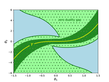
Figure 2. Region of zero duality gap from Figure 1. The darker region is the guaranteed region of zero duality gap (Corollary 3.13).

4. The General Case

We are now ready to consider the general parametrized family of QCQPs (Q), along with their associated SDPs (P) and (D). We assume throughout this section that $F_{\theta},G_{\theta}^{i},c_{\theta}^{i}$ are continuous differentiable functions of $\theta$, and that at least one $c_{\theta}^{i}\!\neq\!0$. Let $\bar{\theta}\!\in\!\Theta$ be a zero duality gap parameter, $\bar{x}\!\in\!{\mathbb{R}}^{N}$ be optimal for ($Q_{\bar{\theta}}$), and $\bar{\lambda}\!\in\!{\mathbb{R}}^{m}$ be optimal for $(D_{\bar{\theta}})$. We denote $\bar{H}:=\mathcal{H}_{\bar{\theta}}(\bar{\lambda})\in{\mathbb{S}}^{N}$ half the Hessian of the Lagrangian at $\bar{\theta}$. Recall that $\bar{H}\succeq 0$ and $\bar{H}\bar{x}=0$. We also denote by $\mathbf{X}_{\theta}:=\{x\!\in\!{\mathbb{R}}^{N}:g_{\theta}(x){=}0\}$ the (primal) feasible set, and $\bar{\mathbf{X}}:=\mathbf{X}_{\bar{\theta}}$.

Our first stability result, Theorem 3.2, relied on two important simplifications: the feasible region $\mathbf{X}_{\theta}$ is independent of $\theta$, and $\operatorname{corank}F_{\bar{\theta}}\!=\!1$. Our main stability result in this section will relax these assumptions.

Let us first allow the feasible set $\mathbf{X}_{\theta}$ to depend on $\theta$. Under the additional assumption that $\mathbf{X}_{\theta}$ moves smoothly as a function $\theta$ (as in Definition 4.1), it is possible to obtain stability (Theorem 4.2).

Definition 4.1.

The mapping $\Theta\rightrightarrows{\mathbb{R}}^{N}$, $\theta\mapsto\mathbf{X}_{\theta}$ is smooth nearby $\bar{w}:=(\bar{\theta},\bar{x})$ if its graph $\mathbf{W}\!:=\!\{(\theta,x):x\!\in\!\mathbf{X}_{\theta}\}$ is a smooth manifold nearby $\bar{w}$, and $\dim_{\bar{w}}\mathbf{W}\!=\!\dim\Theta\!+\!\dim_{\bar{x}}\bar{\mathbf{X}}$.

Theorem 4.2.

Assume that $\bar{H}$ has corank one, ${\mathrm{ACQ}_{\bar{\mathbf{X}}}(\bar{x})}$ holds, and the mapping $\theta\mapsto\mathbf{X}_{\theta}$ is smooth nearby $(\bar{\theta},\bar{x})$. Then (Q) is SDP-stable near $\theta$ and (P) recovers the minimizer.

We will not prove Theorem 4.2 directly, but rather obtain it as a special instance of our main result, in which we also relax the assumption that $\operatorname{corank}\bar{H}\!=\!1$. Relaxing this assumption is challenging. We will replace it by two weaker assumptions.

Definition 4.3.

A point $x\in\bar{\mathbf{X}}$ is a branch point of $\bar{\mathbf{X}}$ with respect to a linear map $\pi:{\mathbb{R}}^{N}\to{\mathbb{R}}^{k}$ if $\ker(\pi)\cap T_{{x}}\bar{\mathbf{X}}\neq 0$, where $T_{{x}}\bar{\mathbf{X}}:=\ker\nabla{g}_{\bar{\theta}}({x})$ is the tangent space of $\bar{\mathbf{X}}$ at ${x}$.

The next definition is non-standard.

Definition 4.4.

The restricted Slater condition holds at $(\bar{x},\bar{\lambda})$ if there exists $\lambda^{\prime}\!\in\!{\mathbb{R}}^{m}$ such that the quadratic function $\Psi_{\lambda^{\prime}}(x):=\sum_{i}\lambda^{\prime}_{i}\,g^{i}_{\bar{\theta}}(x)$ is strictly convex on

$$V\,:=\,\{v\in{\mathbb{R}}^{N}:\bar{H}v\!=\!0,\bar{x}^{\top}v\!=\!0\}\,=\,\ker\bar{H}\cap(\bar{x})^{\perp},$$

and also $\nabla\Psi_{\lambda^{\prime}}(\bar{x})=2\sum_{i}\lambda_{i}^{\prime}G^{i}_{\bar{\theta}}\bar{x}=0$.

We proceed to present our most general result, and afterwards we will discuss the new assumptions in detail.

Theorem 4.5 (Main result).

Assume that:

1. (ACQ) the constraint qualification ${\mathrm{ACQ}_{\bar{\mathbf{X}}}(\bar{x})}$ holds.

2. (smoothness) the mapping $\theta\mapsto\mathbf{X}_{\theta}$ is smooth nearby $(\bar{\theta},\bar{x})$.

3. (non-branch point) $\bar{x}$ is not a branch point of $\bar{\mathbf{X}}$ with respect to $x\mapsto\bar{H}x$.

4. (restricted Slater) the restricted Slater condition holds at $(\bar{x},\bar{\lambda})$.

Then (Q) is SDP-stable near $\bar{\theta}$ and (P) recovers the minimizer.

Theorem 4.2 is a special case of Theorem 4.5, since if $\operatorname{corank}\bar{H}\!=\!1$ then the non-branch point and restricted Slater conditions are satisfied.

4.1. Discussion of the assumptions

Theorem 4.5 has four assumptions. The ACQ and smoothness conditions are concerned with the regularity of the feasible set. ACQ says that the fixed variety $\bar{\mathbf{X}}=\mathbf{X}_{\bar{\theta}}$ is smooth nearby $\bar{x}$, while the smoothness condition ensures that the family of varieties $\mathbf{X}_{\theta}$ behaves well nearby $\bar{\theta}$. We proceed to introduce the remaining two conditions from Theorem 4.5.

4.1.1. Non-branch point

The ACQ property guarantees regularity of the feasible set $\bar{\mathbf{X}}$ nearby $\bar{x}$. In order to guarantee SDP-stability, we will also need regularity of the image of $\bar{\mathbf{X}}$ under the linear map $x\mapsto\bar{H}x$. The next example illustrates the issues we may face when this image is not regular.

Example 4.6.

Consider the nearest point problem to the plane curve $\mathbf{Y}:=\{y\!\in\!{\mathbb{R}}^{2}:y_{2}^{2}\!=\!y_{1}^{3}\}$. By introducing the auxiliary variable $z$ we can rewrite the problem as the inhomogeneous QCQP $\min\{\|y\!-\!\theta\|^{2}:y_{1}\!=\!z^{2},\,y_{2}\!=\!y_{1}z\}$. The feasible set of this QCQP is the twisted cubic curve $\mathbf{X}:=\{(y_{1},y_{2},z):y_{1}{=}z^{2},\,y_{2}{=}z^{3}\}$, which satisfies ACQ everywhere. However, the parameter $\bar{\theta}\!=\!(0,0)$ is problematic for the SDP relaxation (e.g., ($P_{\bar{\theta}}$) has multiple solutions). The underlying cause is that the optimal solution $\bar{y}\!=\!(0,0)$ is a singular point of the plane curve $\mathbf{Y}$. As shown in Figure 3, the singular curve $\mathbf{Y}$ is the projection of $\mathbf{X}$ under the map $(y_{2},y_{3},z)\mapsto(y_{2},y_{3})$. This linear map agrees with $x\mapsto\bar{H}x$ for the point $\bar{\theta}\!=\!(0,0)$.

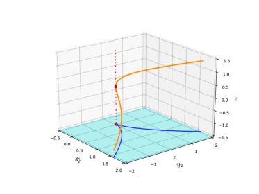
Figure 3. The plane curve $y_{2}^{2}\!=\!y_{1}^{3}$ is the projection of the twisted cubic. The smooth point $(0,0,0)$ is a branch point of the twisted cubic curve with respect to the projection. It maps to the singular point $(0,0)$ on $y_{2}^{2}\!=\!y_{1}^{3}$.

The purpose of the non-branch point assumption is to ensure that $\bar{H}\bar{x}$ is a regular point of $\bar{H}(\bar{\mathbf{X}})$. More generally, consider a linear map $\pi:{\mathbb{R}}^{N}\to{\mathbb{R}}^{k}$ and let $\bar{x}$ be a regular point of $\bar{\mathbf{X}}$ (i.e., ${\mathrm{ACQ}_{\mathbf{X}}(\bar{x})}$ holds). Then regularity of $\pi(\bar{x})$ may only fail when $\bar{x}$ is a branch point of $\pi$ (i.e., if $\ker(\pi)\cap T_{\bar{x}}\bar{\mathbf{X}}\!\neq\!0$).

Example 4.7.

Consider the setup of Example 4.6. The reason why the smooth curve $\mathbf{X}$ is projected into the singular curve $\mathbf{Y}$ is that $\bar{x}=(0,0,0)$ is a branch point of $\mathbf{X}$ with respect to $(y_{1},y_{2},z)\mapsto(y_{1},y_{2})$. This can be observed in Figure 3, by noticing that the tangent line of $\mathbf{X}$ at $\bar{x}$ is precisely the $z$-axis.

4.1.2. Restricted Slater

The previous assumptions (ACQ, smoothness, non-branch point) are all regularity conditions on certain domains (either $\bar{\mathbf{X}}$, $\mathbf{W}$, or $\bar{H}(\bar{\mathbf{X}})$). Importantly, all of these regularity assumptions are satisfied for generic problems. However, they are not enough to guarantee stability of the relaxation, as illustrated by the following example.

Example 4.8 (Non-informative dual).

Consider the following homogeneous QCQP:

$$\min_{z\in{\mathbb{R}}^{3},y\in{\mathbb{R}}^{3}}\;\|y-\theta z_{0}\|^{2},\quad\text{s.t.}\quad z_{0}^{2}=1,\quad z_{1}^{2}+z_{2}^{2}=1,\quad(\begin{smallmatrix}z_{1}&z_{2}\end{smallmatrix})\bigl{(}\begin{smallmatrix}z_{0}&y_{1}&y_{2}\\ y_{1}&y_{2}&y_{3}\end{smallmatrix}\bigr{)}\!=(\begin{smallmatrix}0&0&0\end{smallmatrix}).$$

This is in fact computing the nearest point to the twisted cubic. Indeed, assuming that $z_{0}\!=\!1$, the matrix $\bigl{(}\begin{smallmatrix}z_{0}&y_{1}&y_{2}\\ y_{1}&y_{2}&y_{3}\end{smallmatrix}\bigr{)}$ is rank deficient if and only if $(y_{1},y_{2},y_{3})$ lies on the twisted cubic. A simple calculation shows that the feasible set is regular everywhere (ACQ holds). The feasible set is independent of $\theta$, so the smoothness assumption also holds. As the projection $(z,y)\mapsto y$ leads to the twisted cubic, which is smooth, the non-branch point condition also holds. Nonetheless, we claim that $\operatorname{val}(D_{\theta})\!=\!0$ for any $\theta$, which means that there is zero duality gap only if $\theta$ lies on the twisted cubic. The dual problem (D) involves five variables $\lambda_{0},\lambda_{1},\dots,\lambda_{4}$ corresponding to the five constraints, and has the form:

$$\max_{\lambda\in{\mathbb{R}}^{5}}\;\;-\lambda_{0}-\lambda_{1}\qquad\text{s.t.}\qquad\biggl{(}\begin{smallmatrix}\lambda_{0}+\|\theta\|^{2}&b(\lambda)\!^{\top}&-\theta^{\top}\\ b(\lambda)&\lambda_{1}\!\operatorname{\mathds{1}\mkern-1.0mu}_{2}&B(\lambda)\!^{\top}\\ -\theta&B(\lambda)&\operatorname{\mathds{1}\mkern-1.0mu}_{3}\end{smallmatrix}\biggr{)}\succeq 0,$$

where $b(\lambda)\!\in\!{\mathbb{R}}^{2},B(\lambda)\!\in\!{\mathbb{R}}^{3\times 2}$ depend linearly on $\lambda$. Observe that the cost $-\lambda_{0}{-}\lambda_{1}$ is non-positive for any feasible $\lambda$. Indeed, the constraint $\lambda_{1}\!\operatorname{\mathds{1}\mkern-1.0mu}\succeq 0$ implies $\lambda_{1}\!\geq\!0$, while $\bigl{(}\begin{smallmatrix}\lambda_{0}+\|\theta\|^{2}&-\theta^{\top}\\[-1.0pt] -\theta&\operatorname{\mathds{1}\mkern-1.0mu}\end{smallmatrix}\bigr{)}\succeq 0$ implies $\lambda_{0}\!\geq\!0$. It follows that $\lambda\!=\!0$ is dual optimal, so $\operatorname{val}(D_{\theta})\!=\!0$ for any $\theta$. Note that in this example, $\bar{H}=F_{\bar{\theta}}$ which has corank $>1$ since the objective function does not contain $z_{1},z_{2}$.

The previous example shows that in the absence of the corank-one assumption on $\bar{H}$ the problem may be unstable, even under natural regularity assumptions. We will show in the next section that the restricted Slater assumption allows us to pass from $\bar{\lambda}$ to a different dual optimal solution $\lambda_{t}$ such that $\mathcal{H}_{\bar{\theta}}(\lambda_{t})$ has corank one. This helps to restore stability nearby $\bar{\theta}$.

Unlike the previous regularity conditions, restricted Slater is a semialgebraic condition which is not satisfied generically. Nonetheless, restricted Slater can be verified efficiently as it corresponds to the strict feasibility of an SDP (find $\lambda^{\prime}$ s.t. $\sum_{i}\lambda^{\prime}_{i}G^{i}_{\bar{\theta}}\bar{x}=0$, $(\sum_{i}\lambda^{\prime}_{i}G^{i}_{\bar{\theta}})|_{V}\succ 0$).

Example 4.9.

Let us see that restricted Slater is not satisfied in Example 4.8. Recall that ACQ holds, i.e., $\operatorname{rank}\nabla g_{\bar{\theta}}(\bar{x})=\operatorname{codim}\bar{\mathbf{X}}=5$. The $\lambda^{\prime}$ from Definition 4.4 must satisfy $(\lambda^{\prime})\!^{\top}\nabla g_{\bar{\theta}}(\bar{x})=0$. Since $\nabla g_{\bar{\theta}}(\bar{x})$ has full rank, then $\lambda^{\prime}\!=\!0$. Hence, restricted Slater does not hold.

4.2. Proof of the main theorem

We first see how the vector $\lambda^{\prime}$ from Definition 4.4 gives us a direction along which we can perturb $\bar{\lambda}$ to obtain a new Hessian with corank one.

Lemma 4.10.

Let $(\bar{x},\bar{\lambda})$ be primal/dual optimal at $\bar{\theta}$, and let $\lambda^{\prime}$ be as in Definition 4.4. Then there is an $\epsilon>0$ such that $\lambda_{t}:=\bar{\lambda}+t\lambda^{\prime}$ is dual optimal and $\operatorname{corank}\mathcal{H}_{\bar{\theta}}(\lambda_{t})=1$ for any $0<t<\epsilon$.

The proof of Lemma 4.10 relies on the following well-known lemma.

Lemma 4.11 (Finsler [18]).

Let $A,B\!\in\!{\mathbb{S}}^{n}$, $A\!\succeq\!0$, be such that $v^{\top}Bv\!>\!0$ for every nonzero $v$ with $Av\!=\!0$. Then there is an $\epsilon\!>\!0$ such that $A\!+\!tB\succ 0$ for any $0<t<\epsilon$.

Proof of Lemma 4.10.

Since $(\bar{x},\bar{\lambda})$ is primal/dual optimal, it satisfies the three conditions in Lemma 2.1. We need to show that $(\bar{x},\lambda_{t})$ also satisfies these conditions, and that $\operatorname{corank}\mathcal{H}_{\bar{\theta}}(\lambda_{t})\!=\!1$. Let $A:=\mathcal{H}_{\bar{\theta}}(\bar{\lambda})\succeq 0$ and $B:=\sum_{i}\lambda^{\prime}_{i}G^{i}_{\bar{\theta}}$. Observe that $A\bar{x}\!=\!0$ since $\bar{\lambda}\in\Lambda_{\bar{\theta}}(\bar{x})$, and $B\bar{x}\!=\!0$ by definition of $\lambda^{\prime}$. Since $\mathcal{H}_{\bar{\theta}}(\lambda_{t})\!=\!A{+}tB$ then $\mathcal{H}_{\bar{\theta}}(\lambda_{t})\bar{x}\!=\!0$, so $\lambda_{t}\in\Lambda_{\bar{\theta}}(\bar{x})$. It remains to show that $A{+}tB\succeq 0$ and has corank-one. We may assume without loss of generality that $\bar{x}=(1,0^{N-1})$. Then $A=\bigl{(}\begin{smallmatrix}0&0\\ 0&A^{\prime}\end{smallmatrix}\bigr{)}$, $B=\bigl{(}\begin{smallmatrix}0&0\\ 0&B^{\prime}\end{smallmatrix}\bigr{)}$, where $A^{\prime},B^{\prime}\in{\mathbb{S}}^{N-1}$, $A^{\prime}\succeq 0$. Note that $v^{\top}B^{\prime}v>0$ for every nonzero $v\in{\mathbb{R}}^{N-1}$ with $A^{\prime}v=0$. From Lemma 4.11 we know that $A^{\prime}{+}tB^{\prime}\succ 0$ for all $0<t<\epsilon$. Therefore, $A{+}tB\succeq 0$ and has corank one for $0<t<\epsilon$, as wanted. ∎

Recall that Proposition 3.5 shows that $\operatorname{corank}\mathcal{H}_{\bar{\theta}}(\bar{\lambda})\!=\!1$ implies SDP-stability near $\bar{\theta}$, as long as the Lagrange multiplier mapping satisfies weak continuity. Lemma 4.10 allows us to find a dual optimal solution $\lambda_{t}$ for which $\operatorname{corank}\mathcal{H}_{\bar{\theta}}(\lambda_{t})\!=\!1$. In order to use Proposition 3.5 and conclude SDP-stability, it remains to see that $(\bar{x},\lambda_{t})$ satisfies weak continuity, which can be obtained via a stronger continuity requirement on the original pair $(\bar{x},\bar{\lambda})$. We first recall a well-studied notion of continuity for set-valued-mappings. We refer to [32, 2] for a detailed introduction to set-valued-mappings.

Definition 4.12 (Painlevé-Kuratowski continuity).

Let $\mathfrak{F}:\Theta\rightrightarrows{\mathbb{R}}^{k}$ be a set-valued mapping, and assume that each $\mathfrak{F}(\theta)\subseteq{\mathbb{R}}^{k}$ is nonempty. A selection of $\mathfrak{F}$ is an assignment $\ell_{\theta}\in\mathfrak{F}(\theta)$ for each $\theta\in\Theta$. The inner limit of $\mathfrak{F}$ at $\bar{\theta}$ consists of all limits of selections $\{\ell_{\theta}\}_{\theta}$, i.e.,

$$\liminf_{\theta\to\bar{\theta}}\mathfrak{F}(\theta) :=\{\ell\in{\mathbb{R}}^{k}:\exists\ell_{\theta}\in\mathfrak{F}(\theta)\text{ s.t. }\ell_{\theta}\xrightarrow{\theta\to\bar{\theta}}\ell\},$$

The outer limit of $\mathfrak{F}$ at $\bar{\theta}$ consists of all cluster points of selections $\{\ell_{\theta}\}_{\theta}$, i.e.,

$$\limsup_{\theta\to\bar{\theta}}\mathfrak{F}(\theta) :=\{\ell\in{\mathbb{R}}^{k}:\exists\theta_{i}\xrightarrow{i\to\infty}\bar{\theta},\;\exists\ell_{i}\in\mathfrak{F}(\theta_{i})\text{ s.t. }\ell_{i}\xrightarrow{i\to\infty}\ell\}.$$

The inner and outer limits are always closed sets that sandwich the closure of $\mathfrak{F}({\bar{\theta}})$:

$$\liminf_{\theta\to\bar{\theta}}\mathfrak{F}(\theta)\subseteq\operatorname{cl}(\mathfrak{F}({\bar{\theta}}))\subseteq\limsup_{\theta\to\bar{\theta}}\mathfrak{F}(\theta).$$

$\mathfrak{F}$ is (Painlevé-Kuratowski) continuous at $\bar{\theta}$ if $\mathfrak{F}({\bar{\theta}})=\liminf_{\theta\to\bar{\theta}}\mathfrak{F}(\theta)=\limsup_{\theta\to\bar{\theta}}\mathfrak{F}(\theta).$

Remark 4.13.

When $\mathfrak{F}$ is defined by continuous functions, such as $\mathfrak{L}$, then the equation $\mathfrak{F}({\bar{\theta}})=\limsup_{\theta\to\bar{\theta}}\mathfrak{F}(\theta)$ always holds [32, Ex 5.8]. Consequently, in this paper we will focus our attention only on the inner limit.

Remark 4.14.

Note that weak continuity is simply that $\bar{\ell}=(\bar{x},\bar{\lambda})\in\liminf_{\theta\to\bar{\theta}}\mathfrak{L}(\theta)$.

Example 4.15.

Consider the mapping

$$\mathfrak{F}:{\mathbb{R}}\rightrightarrows{\mathbb{R}},\qquad\theta\mapsto\begin{cases}\{0\},&\text{if }\theta<0\\ [-1,1],&\text{if }\theta\geq 0\end{cases}$$

This mapping is continuous at any $\theta\neq 0$. Observe that $\liminf_{\theta\to 0}\mathfrak{F}(\theta)=\{0\}$ and $\limsup_{\theta\to 0}\mathfrak{F}(\theta)=[-1,1]$. Thus $\mathfrak{F}$ is not continuous at $0$.

Definition 4.16.

The Lagrange multiplier mapping $\mathfrak{L}$ is strongly continuous at a pair $\bar{\ell}=(\bar{x},\bar{\lambda})\in\mathfrak{L}(\bar{\theta})$ if there exists a closed neighborhood $U\ni\bar{\ell}$ such that $\mathfrak{L}(\bar{\theta})\cap U\subseteq\liminf_{\theta\to\bar{\theta}}\mathfrak{L}(\theta)$, or equivalently, such that the mapping $\theta\mapsto\mathfrak{L}(\theta)\cap U$ is continuous at $\bar{\theta}$.

The next proposition shows that the three regularity conditions (ACQ, smoothness, non-branch point) guarantee strong continuity of the multipliers. This proposition can be extended to arbitrary nonlinear programs. The proof relies on the implicit function theorem, but it also requires some technical definitions from variational analysis. Hence we postpone the proof to Appendix A.

Proposition 4.17.

Let $\bar{x}$ be a critical point of ($Q_{\bar{\theta}}$) and $\bar{\lambda}\in\Lambda_{\bar{\theta}}(\bar{x})$. Assume that ${\mathrm{ACQ}_{\bar{\mathbf{X}}}(\bar{x})}$ holds, the mapping $\theta\mapsto\mathbf{X}_{\theta}$ is smooth nearby $(\bar{\theta},\bar{x})$, and $\bar{x}$ is not a branch point of $\bar{\mathbf{X}}$ with respect to $x\mapsto\bar{H}x$. Then strong continuity holds at $(\bar{x},\bar{\lambda})$.

The proof of Theorem 4.5 is now completed by the following theorem, which is the analog of Proposition 3.5.

Proposition 4.18.

Let $(\bar{x},\bar{\lambda})$ be primal/dual optimal at $\bar{\theta}$, such that restricted Slater and strong continuity hold. Then (Q) is SDP-stable near $\bar{\theta}$ and (P) recovers the minimizer.

Proof.

Let $U\ni\bar{\ell}$ be as in Definition 4.16. By Lemma 4.10, there is a dual optimal solution $\lambda_{t}$, arbitrarily close to $\bar{\lambda}$, such that $\mathcal{H}_{\bar{\theta}}(\lambda_{t})$ has corank one. Thus, we may assume that $\ell_{t}:=(\bar{x},\lambda_{t})\in U$. We already saw that $\lambda_{t}$ is a Lagrange multiplier of $\bar{x}$. Therefore, $\ell_{t}$ belongs to $\mathfrak{L}(\bar{\theta})\cap U\subseteq\liminf_{\theta\to\bar{\theta}}\mathfrak{L}(\theta)$. Since $\operatorname{corank}\mathcal{H}_{\bar{\theta}}(\lambda_{t})\!=\!1$ and $\ell_{t}$ satisfies weak-continuity, the theorem follows from Proposition 3.5. ∎

4.3. The inhomogeneous version of the main theorem

Many applications are better suited to an inhomogeneous version of Theorem 4.5, which we now derive.

Theorem 4.19.

Consider the inhomogeneous family of QCQPs:

($$\tilde{Q}_{\theta} \min_{y\in{\mathbb{R}}^{n}}\;\tilde{f}_{\theta}(y)\!:=\!y^{\top}\tilde{F}_{\theta}y\!+\!2\tilde{l}_{\theta}^{\,\top}y\!+\!\tilde{c}_{\theta},\quad\text{s.t.}\quad\tilde{g}_{\theta}^{i}(y)\!:=\!y^{\top}\tilde{G}_{\theta}^{i}y\!+\!2(\tilde{l}_{\theta}^{i})^{\!\top}y\!+\!\tilde{c}_{\theta}^{i}\!=\!0,\;\;i\!=\!1,\ldots,m.$$)

Let $\bar{\theta}$ be a zero duality gap parameter, $(\bar{y},\bar{\mu})$ be the primal/dual optimal solutions at $\bar{\theta}$, and

$$\tilde{\mathcal{H}}_{\theta}(\mu):=\tilde{F}_{\theta}+\sum\nolimits_{i}\mu_{i}\tilde{G}_{\theta}^{i}\in{\mathbb{S}}^{n},\quad\;\;\tilde{H}:=\tilde{\mathcal{H}}_{\bar{\theta}}(\bar{\mu}),\quad\;\;\mathbf{Y}_{\theta}:=\{y\!\in\!{\mathbb{R}}^{n}:\tilde{g}_{\theta}(y){=}0\},\quad\;\;\bar{\mathbf{Y}}:=\mathbf{Y}_{\bar{\theta}}.$$

Assume that the following conditions hold:

1. (ACQ) the constraint qualification ${\mathrm{ACQ}_{\bar{\mathbf{Y}}}(\bar{y})}$ holds.

2. (smoothness) the mapping $\theta\mapsto\mathbf{Y}_{\theta}$ is smooth nearby $(\bar{\theta},\bar{y})$.

3. (non-branch point) $\bar{y}$ is not a branch point of $\bar{\mathbf{Y}}$ with respect to $y\mapsto\tilde{H}y$.

4. (restricted Slater) There exists $\mu^{\prime}\!\in\!{\mathbb{R}}^{m}$ such that the quadratic function $\tilde{\Psi}_{\mu^{\prime}}(y)\!:=\sum_{i}\mu_{i}^{\prime}\tilde{g}^{i}_{\bar{\theta}}(y)$ is strictly convex on $U\!:=\!\ker\tilde{H}$, and also $\nabla\tilde{\Psi}_{\mu^{\prime}}(\bar{y})\!=\!0$.

Then ($\tilde{Q}_{\theta}$) is SDP-stable near $\bar{\theta}$ and the SDP recovers the minimizer.

Proof.

We first argue that we can reduce the problem to the case $\bar{y}\!=\!0$. If this is not the case, then we may consider the change of variables $w:=y{-}\bar{y}$. It is easy to see that that if the conditions from Theorem 4.19 were satisfied for the original problem, then they are also satisfied for the modified problem. Hence, we may assume that $\bar{y}=0$.

The homogenized problem has primal variables $x\!=\!(z_{0},y)$ and dual variables $\lambda\!=\!(\lambda_{0},\mu)$. Note that $\bar{x}\!=\!(1,0)$ since $\bar{y}\!=\!0$. The homogeneous and inhomogeneous problems are related as follows:

$$\nabla g_{\bar{\theta}}(\bar{x})=\biggl{(}\begin{matrix}2&0\\ -\nabla\tilde{g}_{\bar{\theta}}(\bar{y})\bar{y}&\nabla\tilde{g}_{\bar{\theta}}(\bar{y})\end{matrix}\biggr{)},\qquad\qquad\bar{H}=\biggl{(}\begin{matrix}0&0\\ 0&\tilde{H}\end{matrix}\biggr{)},$$

$$\nabla\Psi_{\lambda}(\bar{x})=\biggl{(}\begin{matrix}2\lambda_{0}\!-\!\nabla\tilde{\Psi}_{\mu}(\bar{y})\bar{y}&\nabla\tilde{\Psi}_{\mu}(\bar{y})\end{matrix}\biggr{)},\qquad\nabla^{2}\Psi_{\lambda}=\biggl{(}\begin{matrix}2\lambda_{0}&*\\ *&\nabla^{2}\tilde{\Psi}_{\mu}\end{matrix}\biggr{)}.$$

We proceed to show that ($\tilde{Q}_{\theta}$) satisfies the conditions (i)—(iv) in Theorem 4.19 if and only if its homogenization (Q) satisfies the conditions in Theorem 4.5.

1. $\operatorname{rank}\nabla g_{\bar{\theta}}(\bar{x})=\operatorname{rank}\nabla\tilde{g}_{\bar{\theta}}(\bar{y}){+}1$, $\dim_{\bar{x}}\bar{\mathbf{X}}=\dim_{\bar{y}}\bar{\mathbf{Y}}$, $\operatorname{codim}_{\bar{x}}\bar{\mathbf{X}}=\operatorname{codim}_{\bar{y}}\bar{\mathbf{Y}}{+}1$.

2. $\mathbf{X}_{\theta}=\{(z_{0},y):z_{0}\!=\!\pm 1,\,z_{0}y\!\in\!\mathbf{Y}_{\theta}\}$ consists of two disjoint copies of $\mathbf{Y}_{\theta}$.

3. Notice that $\ker\nabla g_{\bar{\theta}}(\bar{x})=\{0\}\times\ker\nabla\tilde{g}_{\bar{\theta}}(\bar{y})$ and that $\ker\bar{H}={\mathbb{R}}\times\ker\tilde{H}$. The result follows from the equation $\ker\nabla g_{\bar{\theta}}(\bar{x})\cap\ker\bar{H}=\{0\}\!\times\!(\ker\nabla\tilde{g}_{\bar{\theta}}(\bar{y})\cap\ker\tilde{H})$.

4. Let $\mathring{\mu}:=(0,\mu)$ and $\mathring{u}:=(0,u)$ denote the vectors obtained by prepending a zero. Note that

   $$\qquad\nabla{\Psi}_{\mathring{\mu}}(\bar{x})\!=\!0\iff\!\nabla\tilde{\Psi}_{\mu}(\bar{y})\!=\!0,\quad\ker\bar{H}\cap(\bar{x})^{\perp}\!=\{0\}\!\!\times\!\ker\tilde{H},\quad\mathring{u}^{\top}\nabla^{2}{\Psi}_{\mathring{\mu}}\,\mathring{u}=u^{\top}\nabla^{2}\tilde{\Psi}_{\mu}u.$$

   Let $\mu^{\prime}\!\in\!{\mathbb{R}}^{m}$ such that $\nabla\tilde{\Psi}_{\mu}(\bar{y})\!=\!0$ and also $u^{\top}\nabla^{2}\tilde{\Psi}_{\mu^{\prime}}\,u\!>\!0$ for all nonzero $u\!\in\!\ker\tilde{H}$. By the above equations we have that $\lambda^{\prime}\!:=\!\mathring{\mu}^{\prime}$ satisfies $\nabla\Psi_{\lambda^{\prime}}(\bar{x})\!=\!0$ and also $v^{\top}\nabla^{2}\Psi_{\lambda^{\prime}}\,v\!>\!0$ for all nonzero $v\in\ker\tilde{H}\cap(\bar{x})^{\perp}$. The converse implication is similar. ∎

We conclude this section with an illustration of Theorem 4.19 on yet another QCQP on the twisted cubic, but this time, the objective function is nonconvex.

Example 4.20.

Given $\theta\!\in\!{\mathbb{R}}$, consider minimizing $y_{3}^{2}{+}y_{1}y_{3}{-}2\theta y_{1}^{2}{-}2y_{3}$ on the cubic curve defined by $y_{3}\!=\!y_{1}^{3}$. We may rewrite the problem as a QCQP by introducing the auxiliary variable $y_{2}\!=\!y_{1}^{2}$:

(7) $$\min_{y_{1},y_{2},y_{3}\in{\mathbb{R}}}\quad y_{3}^{2}{+}y_{1}y_{3}{-}2\theta y_{1}^{2}{-}2y_{3},\quad\text{ s.t. }\quad y_{2}\!-\!y_{1}^{2}=y_{3}\!-\!y_{1}y_{2}=y_{2}^{2}\!-\!y_{1}y_{3}=0.$$

Consider the nominal parameter $\bar{\theta}\!=\!1$, at which we have $\operatorname{val}(Q_{\bar{\theta}})\!=\!\operatorname{val}(D_{\bar{\theta}})\!=\!-2$. The optimal solutions are $\bar{y}=(1,1,1)$ and $\bar{\mu}=(-2,0,1)$. We claim that the assumptions from Theorem 4.19 hold, and hence the problem is SDP-stable nearby $\bar{\theta}$.

The variety $\bar{\mathbf{Y}}$ is the twisted cubic, so ACQ holds everywhere. The smoothness assumption also holds as the constraints are independent of $\theta$. We proceed to the non-branch point condition. Note that

$$\nabla\tilde{g}(\bar{y})=\left(\begin{smallmatrix}-2&1&0\\ -1&-1&1\\ -1&2&-1\end{smallmatrix}\right),\qquad\tilde{L}_{\bar{\theta}}(y,\bar{\mu})=(y_{2}{-}1)^{2}+(y_{3}{-}1)^{2}-2,\qquad\tilde{H}=\nabla^{2}\tilde{L}_{\bar{\theta}}=\biggl{(}\begin{smallmatrix}0&0&0\\ 0&1&0\\ 0&0&1\end{smallmatrix}\biggr{)}.$$

Then $\ker\nabla\tilde{g}(\bar{y})$ is spanned by $(1,2,3)$, and $\ker\tilde{H}$ by $(1,0,0)$, so $\bar{y}$ is not a branch point. Finally, let us see that restricted Slater holds with $\mu^{\prime}\!=\!(-1,1,1)$. The corresponding quadratic function is $\tilde{\Psi}_{\mu^{\prime}}(y):=y_{1}^{2}{-}y_{1}y_{2}{+}y_{2}^{2}{-}y_{1}y_{3}{-}y_{2}{+}y_{3}$ and one can check that $\nabla\tilde{\Psi}_{\mu^{\prime}}(\bar{y})\!=\!0$. Recall that $U:=\ker\tilde{H}$ is the line spanned by $(1,0,0)$. So the restriction of $\tilde{\Psi}_{\mu^{\prime}}$ to $U$ is the univariate function $y_{1}\mapsto y_{1}^{2}$, which is strictly convex. We have verified the four conditions needed in Theorem 4.19.

5. Applications

We now apply our results to an array of applications. Recall that the motivation for this paper was to provide a theoretical understanding of the observation that many statistical estimation problems exhibit zero duality gap under low noise. Our results provide a uniform framework for understanding these, and other stability results.

5.1. Estimation problems with a strictly convex objective

We first consider two nearest point problems to which we apply Corollary 3.10. This requires checking the ACQ property for which we rely on the following well-known fact (see e.g., [22, §14]).

Lemma 5.1.

Let $g\subseteq{\mathbb{R}}[x]$ be a polynomial system with variety $\mathbf{X}$. If the ideal $\langle g\rangle$ is radical then ACQ holds for each smooth point of $\mathbf{X}$.

Example 5.2 (Triangulation).

In computer vision we represent 3D points by vectors $z=(z_{1},z_{2},z_{3},1)\in{\mathbb{R}}^{4}$, 2D points (images) by vectors $u=(u_{1},u_{2})\in{\mathbb{R}}^{2}$, and cameras by matrices $P\in{\mathbb{R}}^{3\times 4}$. In the triangulation problem we are given $\ell$ cameras $P_{j}\in{\mathbb{R}}^{3\times 4}$ and noisy images $\hat{u}_{j}\in{\mathbb{R}}^{2}$ of an unknown 3D point $z\in{\mathbb{R}}^{4}$, and the goal is to recover $z$. Assuming i.i.d. Gaussian noise, the MLE is given by the nearest point problem:

$$\min_{u\in\mathbf{U}}\quad \sum_{j=1}^{\ell}\|u_{j}-\hat{u}_{j}\|^{2},\quad\text{where}\quad\mathbf{U}:=\{u\in({\mathbb{R}}^{2})^{\ell}:\exists z\in{\mathbb{P}}^{3}\text{ s.t. }u_{j}=\Pi P_{j}{z}\;\text{ for }1\leq j\leq\ell\},$$

where $\Pi:{\mathbb{R}}^{3}\to{\mathbb{R}}^{2}$, $(y_{1},y_{2},y_{3})\mapsto(y_{1}/y_{3},y_{2}/y_{3})$ is the dehomogenization map. The variety $\mathbf{U}$ is known as the multiview variety. If either $\ell\!=\!2$, or $\ell\!\geq\!4$ and the camera centers are not coplanar, then

$$\mathbf{U}=\{u\in({\mathbb{R}}^{2})^{\ell}:\tilde{g}_{ij}(u_{i},u_{j})=0,\;1\leq i<j\leq\ell\},$$

where $\tilde{g}_{ij}$ are quadratic equations known as the epipolar constraints [23]. This description of $\mathbf{U}$ gives a QCQP. The epipolar equations define a radical ideal [23], so ACQ holds at each smooth point (Lemma 5.1). In particular, ACQ holds generically on the variety. Then, by Corollary 3.10, the SDP relaxation of this QCQP solves the problem exactly (generically) under small noise.

The above SDP relaxation was considered in [1], where they also showed exactness under low noise.

Example 5.3 (Tensor PCA).

Consider vectors $\{v^{j}\!\in\!{\mathbb{R}}^{n_{j}}\}_{j=1}^{\ell}$, and let $\theta\in{\mathbb{R}}^{n_{1}\times\cdots\times n_{\ell}}$ be the tensor with entries $\theta_{i_{1}i_{2}\dots i_{\ell}}=v^{1}_{i_{1}}v^{2}_{i_{2}}\dots v^{\ell}_{i_{\ell}}+\zeta_{i_{1}i_{2}\dots i_{\ell}}$, where $\zeta_{i_{1}i_{2}\dots i_{\ell}}$ are random i.i.d. Gaussian variables. Hence, $\theta$ is a noisy estimate of the rank-one tensor $v^{1}\!\otimes\!\cdots\!\otimes\!v^{\ell}$. The tensor PCA problem, also known as rank-one tensor approximation, consists of recovering the vectors $\{v^{j}\}_{j}$ from the tensor $\theta$. The maximum likelihood estimator is obtained by solving the nearest point problem:

(8) $$\min_{y\in\mathbf{Y}}\quad \|y-\theta\|^{2},\quad\text{ where }\quad\mathbf{Y}:=\{y\in{\mathbb{R}}^{n_{1}\times\cdots\times n_{\ell}}:\operatorname{rank}y=1\}.$$

This is a QCQP since $\mathbf{Y}$ is the quadratic Segre variety [22, §9], cut out by the $2\!\times\!2$ minors of the matrix flattenings of $y$. This ideal of minors is radical, so by Lemma 5.1 we have that ACQ holds everywhere except at the origin (the only singular point). Therefore, by Corollary 3.10, the problem is SDP-stable nearby any nonzero $\bar{\theta}\in Y$. In other words, the problem (8) is solved exactly by its SDP relaxation in the low noise regime. The same holds for symmetric tensors, in which case the associated variety is the Veronese, which is also defined by a radical quadratic ideal.

It is possible to derive an equivalent QCQP formulation of (8) involving less variables (so the SDP is cheaper). The idea is to eliminate the last component $v^{\ell}$ from the tensor $y=v^{1}\!\otimes\!\cdots\!\otimes\!v^{\ell}$, obtaining a new problem in terms of the unit norm tensor $x$ proportional to $v^{1}\!\otimes\!\cdots\!\otimes\!v^{\ell-1}$. This leads to the homogeneous QCQP:

(9) $$\min_{x\in\mathbf{X}}\quad\frac{1}{2}\,\sum_{k=1}^{n_{\ell}}\sum_{I\neq J}(x_{I}\theta_{J,k}-x_{J}\theta_{I,k})^{2},\quad\text{ where }\quad\textbf{X}=\{x\in{\mathbb{R}}^{n_{1}\times\dots\times n_{\ell-1}}\!:\operatorname{rank}x\!=\!1,\;\|x\|^{2}\!=\!1\},$$

and where $I,J$ range over all tuples in $[n_{1}]\times\dots\times[n_{\ell-1}]$. One can check that the assumptions of Theorem 3.2 are satisfied, so the SDP relaxation of (9) is also exact under low noise.

SDP relaxations for the Tensor PCA problem were first studied in [30], where they introduced the idea of eliminating one component for efficiency. Their derivation relies on a parametrization of X, but the SDP is the same as the one obtained with the implicit description. No exactness results were known before.

We now show applications of Theorem 3.9. Note that this theorem has three assumptions: at the nominal parameter $\bar{\theta}$, the objective is strictly convex, ACQ holds for the minimizer, which is also the global minimum of the objective function. Since in the problems below the objective function is a squared loss function, and since in the noiseless case the objective value is zero, the last condition is always satisfied. Thus, we will only check strict convexity and ACQ.

Example 5.4 ($SO(d)$ synchronization).

Consider $n{+}1$ objects in ${\mathbb{R}}^{d}$, whose orientation is described by matrices $R_{i}\!\in\!SO(d)$, where $SO(d)$ is the special orthogonal group. Let $G=(V,E)$ be a graph with vertex set $V=\{0,\dots,n\}$. In the $SO(d)$ synchronization problem we are given noisy estimates $\hat{R}_{ij}\approx R_{j}R_{i}^{\top}$ of the relative orientation among pairs $ij\in E$, and the goal is to recover the matrices $R_{i}$. Under an appropriate noise model [33], the MLE is given by the following least-squares problem:

(10) $$\min_{R_{1},\dots,R_{n}\in SO(d)}\,\sum_{ij\in E}\|R_{j}\!-\!\hat{R}_{ij}R_{i}\|_{F}^{2},\quad\;\;SO(d):=\{R\!\in\!{\mathbb{R}}^{d\times d}:R^{\top}R\!=\!\operatorname{\mathds{1}\mkern-1.0mu}_{d},\;\det(R)\!=\!1\},$$

where we assume that $R_{0}:=\operatorname{\mathds{1}\mkern-1.0mu}_{n}$ is the reference point. This problem is parametrized by $\theta=(\hat{R}_{ij})_{ij\in E}$. To obtain a QCQP, we can replace $SO(d)$ by the orthogonal group $O(d)$:

(11) $$\min_{R_{1},\dots,R_{n}\in O(d)}\;\sum_{ij\in E}\|R_{j}-\hat{R}_{ij}R_{i}\|_{F}^{2},\qquad O(d):=\{R\in{\mathbb{R}}^{d\times d}:R^{\top}R=\operatorname{\mathds{1}\mkern-1.0mu}_{d}\}.$$

Note that (10) and (11) have the same minimizer in the low noise regime, as $SO(d)^{n}$ is a connected component of $O(d)^{n}$. Consider the SDP relaxation of the QCQP (11). The objective function is strictly convex by Lemma 5.5 below, and ACQ is satisfied everywhere since the variety is smooth and the ideal is radical (Lemma 5.1). Thus problem (11) (and hence (10)) is solved exactly by its Lagrangian relaxation in the low noise regime. We point out that problem (11) has a very special structure, so its Lagrangian dual admits a more concise representation than a typical QCQP, see [33, §4.2].

Lemma 5.5.

Let $G=(V,E)$ be a connected graph, let $x_{0}\in{\mathbb{R}}^{k}$, and let $L_{ij}:{\mathbb{R}}^{k}\to{\mathbb{R}}^{k}$ be invertible linear maps for $ij\in E$. Then the function $f(x):=\sum_{ij\in E}\|x_{j}-L_{ij}x_{i}\|^{2}$, where $x=(x_{1},\dots,x_{n})\in({\mathbb{R}}^{k})^{n}$, is strictly convex.

Proof.

We may assume that the reference point $x_{0}\!=\!0$ after a possible affine transformation. Since ${f}(x)$ is convex and homogeneous, it suffices to see that ${f}(x)\!=\!0$ implies $x\!=\!0$. If ${f}(x)\!=\!0$ then $x_{j}\!=\!L_{ij}x_{i}$ for each $ij\!\in\!E$. Since ${x}_{0}\!=\!0$ and $G$ is connected it is clear that each $x_{i}$ must be zero. ∎

An alternative QCQP formulation for the $SO(3)$ synchronization problem can be obtained by representing rotations with quaternions [19]. The same analysis as above shows that the corresponding SDP relaxation is exact in the low noise regime, as was observed experimentally in [19]. Tightness results for $SO(3)$ synchronization similar to ours were obtained in [15, 37].

Example 5.6 ($SE(d)$ synchronization).

A natural extension of the above problem is to replace rotation matrices by elements of the special Euclidean group $SE(d)$. Given a graph $G=(V,E)$, and $\hat{R}_{ij}\in{\mathbb{R}}^{d\times d},\hat{u}_{ij}\in{\mathbb{R}}^{d}$ for $ij\in E$, the problem is

(12) $$\min_{R_{i}\in SO(d),\,u_{i}\in{\mathbb{R}}^{d}}\quad\sum_{ij\in E}\|R_{j}\!-\!\hat{R}_{ij}R_{i}\|_{F}^{2}+\|u_{j}\!-\!u_{i}\!-\!R_{i}\hat{u}_{ij}\|^{2},$$

where $R_{0}:=\operatorname{\mathds{1}\mkern-1.0mu}_{d},u_{0}:=0$. As before, we can replace $SO(d)$ with $O(d)$ to obtain a QCQP, and consider its SDP relaxation. An argument similar to Lemma 5.5 shows that the objective function is strictly convex, and thus the Lagrangian relaxation solves problem (12) exactly under low noise.

SDP relaxations for $SE(d)$ synchronization have received considerable attention in past years and similar exactness results have been derived [33, 37].

Example 5.7 (Orthogonal Procrustes).

Given $n,k,m_{1},m_{2}\!\in\!{\mathbb{N}}$ and matrices $A\!\in\!{\mathbb{R}}^{m_{1}\times n}$, $B\!\in\!{\mathbb{R}}^{m_{1}\times m_{2}}$, $C\!\in\!{\mathbb{R}}^{k\times m_{2}}$, the weighted orthogonal Procrustes problem, is

(13) $$\min_{X\in{\mathbb{R}}^{n\times k}}\quad \|AXC-B\|_{F}^{2},\quad\text{ s.t. }\quad X^{\top}X=\operatorname{\mathds{1}\mkern-1.0mu}_{k}.$$

The above is a QCQP parametrized by $\theta=(A,B,C)$. ACQ holds everywhere since the variety (the Stiefel manifold) is smooth and the ideal is radical. The objective function is strictly convex as long as the linear map $X\mapsto AXC$ is injective. In such cases Theorem 3.9 guarantees that the SDP relaxation is exact under low noise.

Problem (13) may have several local optima, and thus local methods may fail [35, 10]. The above SDP relaxation was considered in [13].

5.2. Estimation problems with degenerate objective

The previous applications had strictly convex objective functions, and hence the theorems from Section 3 were sufficient to analyze them. The results from Section 4 can be used to study much more general estimation problems. A preprint of this paper first appeared on the arXiv in 2017 and has since spawned a number of follow ups [11, 40, 12]. For example [11, 40] used our Theorem 4.5 to establish stability for a number of estimation problems from computer vision, control theory, and symbolic computation. As can be seen from these papers, verifying the assumptions of Theorem 4.5 is non-trivial. So, we briefly mention a few of these applications (without proofs) to give the reader with a sense of how Theorem 4.5 can be used. Several of these are nearest point problems of the form (1) from the Introduction.

Example 5.8 (Essential matrix estimation [40]).

A calibrated camera is described by a matrix of the form $P\!=\!(R\,|\,t)$, with $R\!\in\!SO(3)$, $t\!\in\!{\mathbb{R}}^{3}$. Consider images $(u_{j})_{j=1}^{\ell}\subseteq{\mathbb{R}}^{2}$ and $(u_{j}^{\prime})_{j=1}^{\ell}\subseteq{\mathbb{R}}^{2}$ of the same 3D points under two calibrated cameras $P,P^{\prime}$. The relationship between the image sets $(u_{j})$ and $(u_{j}^{\prime})$ is encoded by the essential matrix $E$. This is a special $3\!\times\!3$ matrix that depends on $P,P^{\prime}$. The problem of estimating an essential matrix $E$ based on noisy estimates $(\hat{u}_{j}),(\hat{u}_{j}^{\prime})$ of the images can be formulated as follows:

$$\min_{E\in{\mathbb{R}}^{3\times 3},\,t\in{\mathbb{R}}^{3}}\quad\sum_{j=1}^{\ell}\|\hat{v}_{j}^{\top}E\,\hat{v}_{j}^{\prime}\|^{2},\quad\text{ s.t. }\quad EE^{\top}=[t]_{\times}[t]_{\times}^{\top}\,,\quad t^{\top}t=1,$$

where $\hat{v}_{j},\hat{v}_{j}^{\prime}\in{\mathbb{R}}^{3}$ are the homogenizations of $\hat{u}_{j},\hat{u}_{j}^{\prime}$, obtained by adding a last coordinate equal to one, and $[t]_{\times}\!\in{\mathbb{R}}^{3\times 3}$ is the skew-symmetric matrix, whose non-zero entries are $\pm t_{i}$, representing cross product with $t$. The above is a homogeneous QCQP in variables $E,t$, parametrized by $\theta=(\hat{v}_{j},\hat{v}_{j}^{\prime})_{j=1}^{\ell}$. The objective is degenerate (its Hessian has corank $3$) as it does not involve $t$, so we cannot apply the results from Section 3. Nonetheless, it is shown in [40] that the assumptions of Theorem 4.5 hold, and hence this problem is solved exactly by the SDP relaxation under low noise.

The sum-of-squares (SOS) method provides a hierarchy of SDP relaxations of a QCQP, in which the first level is the Lagrangian relaxation. Our methods can be used to analyze the SDP relaxations at any level, as will be discussed in more detail in Section 6. The remaining examples illustrations this.

Example 5.9 (Approximate system realization [11]).

Consider a discrete linear time invariant (LTI) system of order $k$. Let $y=(y_{1},y_{2},y_{3},\dots,y_{n})$ be the truncated impulse response of the system, and assume that the signal $y$ is corrupted by Gaussian noise. The approximate realization problem consists of recovering the transfer function of the $k$-th order system from the corrupted signal $\hat{y}$. The MLE can be found by solving the following least squares problem:

$$\min_{y\in{\mathbb{R}}^{n}\!,\,z\in{\mathbb{R}}^{k+1}}\;\|y-\hat{y}\|^{2},\quad\text{ s.t. }\quad z^{\top}H_{k+1}(y)=0,$$

where $H_{k+1}(y)$ is the $(k{+}1)\!\times\!(n{-}k)$ Hankel matrix with the entries of $y$. In particular, the transfer function of the system can be recovered from the optimal $z$. The above problem is an inhomogeneous QCQP in variables $y,z$, parametrized by $\theta\!=\!\hat{y}$. Unfortunately, its Lagrangian relaxation does not provide any information about the value of the QCQP (c.f., Example 4.8). On the other hand, the second level of the SOS hierarchy always solves the problem exactly in the low noise regime. This result is proved in [11] by relying on Theorem 4.5 (as the objective is degenerate, we cannot use Theorem 3.2).

Example 5.10 (Camera resectioning [11]).

In the uncalibrated resectioning problem we are given $\ell$ points $z_{j}\!\in\!{\mathbb{R}}^{4}$ and noisy images $\hat{u}_{j}\!\in\!{\mathbb{R}}^{2}$ under an unknown camera $P\!\in\!{\mathbb{R}}^{3\times 4}$, and the goal is to recover $P$. Assuming i.i.d. Gaussian noise, the MLE is given by

$$\min_{P\in{\mathbb{R}}^{3\times 4},u_{j}\in{\mathbb{R}}^{2}}\quad\sum_{j=1}^{\ell}\|u_{j}-\hat{u}_{j}\|^{2},\quad\text{ s.t. }\quad u_{j}=\Pi Pz_{j}\;\text{ for }j\in[\ell].$$

where $\Pi:{\mathbb{R}}^{2}\to{\mathbb{R}}^{2}$, $(y_{1},y_{2},y_{3})\mapsto(y_{1}/y_{3},y_{2}/y_{3})$. Though this problem looks similar to triangulation (Example 5.2), it is significantly harder because we cannot easily eliminate the auxiliary variables $P$. The above problem can be formulated as a QCQP in the variables $P,u_{j}$ after clearing denominators. As before, the Lagrangian relaxation is non-informative. However, the SDP relaxation in the second level of the SOS hierarchy is always exact in the low noise regime, as shown in [11] by using Theorem 4.5.

Example 5.11 (Approximate GCD [11]).

Let $f_{1}\!\in\!{\mathbb{R}}[t]_{n_{1}}$, $f_{2}\!\in\!{\mathbb{R}}[t]_{n_{2}}$ be univariate polynomials of degrees $n_{1},n_{2}$, and let $g\!\in\!{\mathbb{R}}[t]_{d}$ be their GCD, of degree $d$. Here ${\mathbb{R}}[t]_{k}$ denotes the vector space of univariate polynomials in $t$ of degree at most $k$. The approximate GCD problem consists of estimating the degree $d$ polynomial $g$ from noisy estimates $\hat{f}_{1},\hat{f}_{2}$. The MLE under Gaussian noise is:

$$\min_{f_{1}\in{\mathbb{R}}[t]_{n_{1}},\,f_{2}\in{\mathbb{R}}[t]_{n_{2}},z\in{\mathbb{R}}^{k}}\quad \|f_{1}-\hat{f}_{1}\|^{2}+\|f_{2}-\hat{f}_{2}\|^{2},\quad\text{ s.t. }\quad z^{\top}\operatorname{Syl}_{d}(f_{1},f_{2})=0,$$

where $k:=n_{1}{+}n_{2}{-}2d$, and $\operatorname{Syl}_{d}(f_{1},f_{2})$ is the $k\times(k{+}d{-}1)$ Sylvester matrix, which is filled with the coefficients of $f_{1},f_{2}$; see e.g., [24]. The GCD polynomial $g$ can be read from the vector $z$. It is shown in [11], using Theorem 4.5, that the SDP relaxation in the second level of the SOS hierarchy is exact under low noise.

6. SDP Stability in Polynomial Optimization

Although the main focus of this paper has been the Lagrangian relaxation of a QCQP, the techniques from this paper can be used in much greater generality. In this section, we illustrate how to use our theorems to analyze SDP relaxations of polynomial optimization problems arising from the sum-of-squares (SOS) method.

We first consider unconstrained polynomial optimization. Let ${\mathbb{R}}[z]_{2d}$ be the vector space of multivariate polynomials of degree at most $2d$ in variables $z=(z_{1},\ldots,z_{n})$. Consider the parametric family of unconstrained polynomial optimization problems:

($$\mathit{POP}_{\theta} \min_{z\in{\mathbb{R}}^{n}}\;p_{\theta}(z),\qquad\text{ where }p_{\theta}\in{\mathbb{R}}[z]_{2d}\text{ depends continuously on }\theta.$$)

We will analyze the stability of the SOS relaxation of $(\textit{{POP}\textsubscript{\texttheta}})$.

We briefly review the SOS method. A polynomial $f\in{\mathbb{R}}[z]_{2d}$ is SOS if it can be written in the form $f(z)=\sum_{i}f_{i}(z)^{2}$ for some $f_{i}\in{\mathbb{R}}[z]_{d}$. The set

$$\Sigma_{n,2d}:=\{f\in{\mathbb{R}}[z]_{2d}:f(z)\text{ is SOS }\}$$

is a closed convex cone in ${\mathbb{R}}[z]_{2d}$. The SOS relaxation of ($\mathit{POP}_{\theta}$) is

($$\mathit{SOS}_{\theta} \max_{\gamma\in{\mathbb{R}}}\;\gamma,\quad\text{ s.t. }\quad p_{\theta}(z)-\gamma\in\Sigma_{n,2d}.$$)

Since not all nonnegative polynomials are SOS, we have that $\textup{val}(\textit{{POP}\textsubscript{\texttheta}})\geq\textup{val}(\textit{{SOS}\textsubscript{\texttheta}})$. The relaxation $(\textit{{SOS}\textsubscript{\texttheta}})$ can be solved efficiently with an SDP, and it is tight at $\theta$ if $\operatorname{val}(\mathit{SOS}_{\theta})=\operatorname{val}(\mathit{POP}_{\theta})$. If the minimizer of $p_{\theta}$ is unique, it might also be possible to recover it from the relaxation.

Assume that the SOS relaxation is tight for a specific parameter $\bar{\theta}$. We investigate the behavior of $(\mathit{SOS}_{\theta})$ when $\theta$ is close to $\bar{\theta}$. As the following example shows, stability is not to be taken for granted.

Example 6.1.

For the polynomial $p_{\theta}(z):=z_{1}^{4}z_{2}^{2}+z_{1}^{2}z_{2}^{4}+\theta z_{1}^{2}z_{2}^{2}\in{\mathbb{R}}[z]_{6}$ we have:

$$\theta\geq 0\quad\implies\quad\operatorname{val}(\mathit{POP}_{\theta})=\operatorname{val}(\mathit{SOS}_{\theta})=0,$$

$$\theta<0\quad\implies\quad\operatorname{val}(\mathit{POP}_{\theta})=\tfrac{1}{27}\theta^{3}\text{ and \eqref{eq:sos} is infeasible}.$$

Hence the relaxation is not stable nearby $\bar{\theta}=0$.

We will use Theorem 3.2 to establish a result that guarantees tightness of ($\mathit{SOS}_{\theta}$) near $\bar{\theta}$. The hypothesis for this theorem is a geometric condition involving $p_{\bar{\theta}}$ and the SOS cone $\Sigma_{n,2d}$, which we first explain. Let $\bar{z}$ be the minimizer of $p_{\bar{\theta}}$. Consider the following linear subspaces of ${\mathbb{R}}[z]_{2d}$:

$$H_{\bar{z}}:=\{f\!\in\!{\mathbb{R}}[z]_{2d}:f(\bar{z})\!=\!0\},\qquad L_{\bar{z}}:=\{f\!\in\!{\mathbb{R}}[z]_{2d}:f(\bar{z})\!=\!0,\,\nabla f(\bar{z})\!=\!0\}.$$

The subspace $H_{\bar{z}}$ is defined by a single linear equation, so it is a hyperplane. The intersections of the SOS cone with both subspaces agree. Indeed, if $f(\bar{z})\!=\!0$ and $f$ is SOS, then we must have that $\nabla f(\bar{z})\!=\!0$. Let $K_{\bar{z}}$ be the (exposed) face of the SOS cone given by this intersection:

$$K_{\bar{z}}\,:=\,\Sigma_{n,2d}\cap H_{\bar{z}}\,=\,\Sigma_{n,2d}\cap L_{\bar{z}}.$$

Observe that $p_{\bar{\theta}}\!-\!\bar{\gamma}\in K_{\bar{z}}$, where $\bar{\gamma}:=p_{\bar{\theta}}(\bar{z})$ is the optimal value of $(\mathit{POP}_{\theta})$.

Theorem 6.2.

Let $\bar{\theta}$ be such that $\bar{\gamma}:=\operatorname{val}(\mathit{POP}_{\bar{\theta}})=\operatorname{val}(\mathit{SOS}_{\bar{\theta}})$ and there is a unique minimizer $\bar{z}$. Consider the face $K_{\bar{z}}$ of the cone $\Sigma_{n,2d}$, from above. If $p_{\bar{\theta}}-\bar{\gamma}$ lies in the relative interior of $K_{\bar{z}}$, then the relaxation ($\mathit{SOS}_{\theta}$) is tight and recovers the minimizer whenever $\theta$ is close enough to $\bar{\theta}$.

Proof.

We may assume WLOG that $\bar{\gamma}\!=\!0$, and thus $p_{\bar{\theta}}\in K_{\bar{z}}$. In order to use our methods, we need to rephrase ($\mathit{POP}_{\theta}$) as a QCQP. Let

$$x:=(z^{\alpha})_{\alpha\in J}\in({\mathbb{R}}[z]_{d})^{N},\quad\text{ where }\quad J:=\{\alpha\in{\mathbb{N}}^{n}:\textstyle\sum_{i}\alpha_{i}\leq d\},\quad N:=\binom{n+d}{d},$$

be the vector with all monomials in ${\mathbb{R}}[z]$ of degree at most $d$. Note that any $p\!\in\!{\mathbb{R}}[z]_{2d}$ can be written in the form $p(z)\!=\!x^{\top}Fx$ for some $F\!\in\!{\mathbb{S}}^{N}$. Such an $F$ is called a Gram matrix of $p$. Moreover, $p$ is SOS if and only if it has a positive semidefinite Gram matrix.

Let $\bar{x}\!\in\!{\mathbb{R}}^{N}$ be given by evaluating each of the monomials in $x$ at $\bar{z}$. We first argue that if $p_{\bar{\theta}}\in\operatorname{int}K_{\bar{z}}$, then

1. $p_{\bar{\theta}}$ has a Gram matrix $\bar{F}$ such that $\bar{F}\!\succeq\!0$, $\bar{F}\bar{x}\!=\!0$, and $\operatorname{corank}\bar{F}\!=\!1$.

2. $F_{\theta}:=\phi^{\dagger}(p_{\theta}\!-\!p_{\bar{\theta}})+\bar{F}$ is a Gram matrix of $p_{\theta}$, where $\phi^{\dagger}$ is the pseudo-inverse of the linear map $\phi:{\mathbb{S}}^{N}\to{\mathbb{R}}[z]_{2d}$,  $A\mapsto x^{\top}Ax$.

Observe that $F$ is a Gram matrix of $p$ if and only if $\phi(F)\!=\!p$. Hence (ii) follows by checking that $\phi(F_{\theta})\!=\!p_{\theta}$. Also note that $K_{\bar{z}}\!=\!\phi(S)$, where $S:=\{F\!\in\!{\mathbb{S}}^{N}:F\!\succeq\!0,F\bar{x}\!=\!0\}$. Indeed, $F\succeq 0$ if and only if $f(z)\!:=\!x^{\top}Fx\!\in\!\Sigma_{n,2d}$, in which case $\nabla f(\bar{z})\!=\!2F\bar{x}$, and hence $F\bar{x}\!=\!0$ if and only if $\nabla f(\bar{z})\!=\!0$. Since linear maps preserve relative interiors of convex sets, then $\operatorname{int}K_{\bar{z}}=\phi(\operatorname{int}S)$. Then (i) follows by noticing that $\operatorname{int}S=\{F\!\in\!S:\operatorname{corank}F{=}1\}$.

The above properties provide a family of Gram matrices $F_{\theta}$ that depends continuously on $\theta$. Thus the parametric optimization problem ($\mathit{POP}_{\theta}$) can be phrased as

$$\min_{x\in\mathbf{X}}\;x^{\top}F_{\theta}x,\;\;\quad\text{where}\quad\;\;\mathbf{X}:=\{x\!=\!(z^{\alpha})_{\alpha\in J}:z\in{\mathbb{R}}^{n}\}\subseteq{\mathbb{R}}^{N}.$$

The above is a QCQP since $\mathbf{X}$, the Veronese variety, is defined by quadratic equations:

$$\mathbf{X}:=\{x\in{\mathbb{R}}^{N}:x_{0}\!=\!1,\;x_{\alpha_{1}}x_{\alpha_{2}}\!=\!x_{\beta_{1}}x_{\beta_{2}}\;\;\forall\alpha_{1},\alpha_{2},\beta_{1},\beta_{2}\in J\text{ s.t. }\alpha_{1}\!+\!\alpha_{2}\!=\!\beta_{1}\!+\!\beta_{2}\}.$$

Moreover, the relaxation ($\mathit{SOS}_{\theta}$) coincides with the Lagrangian dual of the above QCQP.

By construction we know that $F_{\bar{\theta}}\!\succeq\!0$, $F_{\bar{\theta}}\bar{x}\!=\!0$, $\operatorname{corank}F_{\bar{\theta}}\!=\!1$. It is known that the Veronese variety is smooth and its ideal is radical. Hence ACQ holds everywhere by Lemma 5.1. The result now follows from Theorem 3.2, ∎

Our techniques can also be applied to constrained polynomial optimization, as we briefly explain. Consider the parametric family of polynomial optimization problems:

($$\mathit{POP}_{\theta}^{\textup{con}} \min_{x\in{\mathbb{R}}^{N}}\quad p_{\theta}(z),\qquad\text{s.t.}\qquad q_{\theta}^{i}(z)\!=\!0,\;\;i\!=\!1,\dots,m,$$)

where $p_{\theta},q_{\theta}^{i}\in{\mathbb{R}}[z]_{2d}$ depend continuously on $\theta$. Given $D\geq d$, the $D$-th order SOS relaxation is:

($$\mathit{SOS}_{\theta}^{\textup{con}} \max_{\gamma\in{\mathbb{R}},\;h^{i}\in{\mathbb{R}}[z]}\;\gamma,\qquad\text{s.t.}\qquad p_{\theta}(z)-\gamma-\sum_{i}h^{i}(z)\,q^{i}_{\theta}(z)\,\in\,\Sigma_{n,2D},$$)

where the optimization variables are the scalar $\gamma\!\in\!{\mathbb{R}}$ and the polynomials $h^{i}\!\in\!{\mathbb{R}}[z]_{2D-2d}$. The relaxation ($\mathit{SOS}_{\theta}^{\textup{con}}$) can be efficiently solved with an SDP. We can use Theorem 4.5 to analyze the stability of this relaxation. In order to do that, we phrase ($\mathit{POP}_{\theta}^{\textup{con}}$) as a QCQP, as before. Namely, express the polynomials $p_{\theta}(z),q_{\theta}^{i}(z)$ as quadratic functions $f_{\theta}(x),g_{\theta}^{i}(x)$ in $x$, where $x\in{\mathbb{R}}^{\binom{n+D}{D}}$ lies in the Veronese variety.

7. Conclusion

Theorems 3.2 and 4.5 guarantee SDP-stability for a parametrized family of QCQPs near a nominal parameter $\bar{\theta}$ at which there is zero duality gap. These results provide a uniform framework within which to understand and explain several previously observed occurrences of zero duality gap under low noise. While the conditions of Theorem 3.2 are relatively easily to check, Theorem 4.5 requires technical assumptions that are more involved. We believe that all the requirements in Theorem 4.5 are necessary for stability.

Our results strongly depend on the quadratic nature of the problem. Although the conditions in Theorems 3.9 and 4.5 make sense for general nonlinear programs, they only guarantee stability of zero duality gap in the QCQP case. For instance, the problem $\min\{x_{1}^{2}\!+\!x_{2}^{2}\!+\!\theta x_{2}^{4}:x_{2}{=}0\}$ satisfies the assumptions of Theorem 3.9 for $\bar{\theta}{=}0$, but the duality gap is not stable (it is zero only at $\bar{\theta}$).

Our stability theorems not only guarantee zero duality gap nearby $\bar{\theta}$, but also that the relaxation recovers the minimizer of the problem. To do so, our theorems assume that the primal and dual optimal values are achieved at the nominal parameter $\bar{\theta}$. We leave for future work to investigate SDP stability in settings where the optimal values are not achieved.

As we have seen several times in this paper, polynomial optimization problems can be formulated as QCQPs by adding extra variables. If these QCQPs satisfy the conditions of our theorems then they exhibit stability. As illustrated by Examples 1.1 and 4.8, different QCQP formulations of the same problem might have different stability properties. It is natural to ask how to choose the best QCQP formulation. The SOS method gives a systematic procedure for constructing a hierarchy of QCQP formulations, and it is optimal in the sense that it includes all valid relations up to a certain degree. The Lagrangian relaxations studied in this paper correspond to the first SOS relaxation. However, the methods of this paper are general and they can be used to study higher order SOS relaxations also. In particular, Theorem 4.5 was used in [11] to analyze the second order SOS relaxation of some of the examples in Section 5.2.

In this paper we have focused on equality-constrained QCQPs. As is standard in nonlinear programming, the results can be extended to account for inequality constraints as long as the active constraints are preserved by the perturbation. A comprehensive treatment of the inequality-constrained case is left for future work.

Acknowledgments

We would like to thank Dmitriy Drusvyatskiy for many helpful conversations, and for suggesting the use of the implicit function theorem to analyze our problem. Diego Cifuentes was in the Laboratory for Information and Decision Systems during the development of this paper. Rekha Thomas was partially supported by the NSF grant DMS-1719538. This work was done in part while Pablo Parrilo was visiting the Simons Institute for the Theory of Computing. It was partially supported by the DIMACS/Simons Collaboration on Bridging Continuous and Discrete Optimization through NSF Grant CCF-1740425. This work was also supported in part by the Air Force Office of Scientific Research through AFOSR Grants FA9550-11-1-0305 and the National Science Foundation through NSF Grant CCF-1565235.

Appendix A Stability of Lagrange multipliers

The goal of this section is to show a generalization of Proposition 4.17 to parametric nonlinear programming. Let $\Theta\subseteq{\mathbb{R}}^{d}$ be the parameter space, let $f:\Theta\times{\mathbb{R}}^{N}\to{\mathbb{R}}$ and $g:\Theta\times{\mathbb{R}}^{N}\to{\mathbb{R}}^{m}$ be continuously differentiable, and such that $f_{\theta},g_{\theta}$ are twice continuously differentiable. Consider the parametric family of nonlinear programs

$$\min_{x\in\mathbf{X}_{\theta}}\quad f_{\theta}(x),\quad\text{ where }\quad\mathbf{X}_{\theta}:=\{x\in{\mathbb{R}}^{N}:g_{\theta}(x)=0\}.$$

Let $L_{\theta}(x,\lambda):=f_{\theta}(x)\!+\!\lambda^{\top}g_{\theta}(x)$ be the Lagrangian function, and let

$$\mathfrak{L}:\Theta\rightrightarrows{\mathbb{R}}^{N}\times{\mathbb{R}}^{m},\qquad\theta\mapsto \{(x,\lambda):g_{\theta}(x)\!=\!0,\;\nabla_{x}L_{\theta}(x,\lambda)\!=\!0\}$$

be the Lagrange multiplier mapping. Let $(\bar{x},\bar{\lambda})\in\mathfrak{L}(\bar{\theta})$ be a Lagrange multiplier pair at the nominal parameter $\bar{\theta}$. We denote $\bar{H}\!:=\!\frac{1}{2}\nabla^{2}_{xx}L_{\bar{\theta}}(\bar{x},\bar{\lambda})$. We will derive conditions that ensure local stability of $\mathfrak{L}$ nearby $\bar{\theta}$. The notion of stability we use is the Aubin property; see [14, 32].

Definition A.1 (Aubin property).

Let $\mathfrak{F}:{\mathbb{R}}^{d}\rightrightarrows{\mathbb{R}}^{n}$ be a set-valued mapping. $\mathfrak{F}$ has the Aubin property at $\bar{p}\!\in\!{\mathbb{R}}^{d}$ for $\bar{y}\!\in\!{\mathbb{R}}^{n}$ if $\bar{y}\!\in\!\mathfrak{F}(\bar{p})$ and there is a constant $\kappa\!\geq\!0$ and neighborhoods $U\!\ni\!\bar{y},V\!\ni\!\bar{p}$ such that

$$\mathfrak{F}(p^{\prime})\cap U\,\subseteq\,\mathfrak{F}(p)+\kappa\,|p^{\prime}\!-\!p|\,\mathcal{B}\quad\mbox{ for all }p^{\prime},p\in V,$$

where $\mathcal{B}\subseteq{\mathbb{R}}^{n}$ denotes the unit ball.

The following is the main result of this section.

Theorem A.2 (Stability of Lagrange multipliers).

Let $(\bar{x},\bar{\lambda})\in\mathfrak{L}(\bar{\theta})$. Assume that ${\mathrm{ACQ}_{\bar{\mathbf{X}}}(\bar{x})}$ holds, the mapping $\theta\mapsto\mathbf{X}_{\theta}$ is smooth nearby $(\bar{\theta},\bar{x})$, and $v^{\top}\bar{H}v\neq 0$ for all nonzero $v\in T_{\bar{x}}(\mathbf{X}_{\bar{\theta}}):=\ker\nabla g_{\bar{\theta}}(\bar{x})$. Then the mapping $\mathfrak{L}$ has the Aubin property at $\bar{\theta}$ for $(\bar{x},\bar{\lambda})$.

Remark A.3.

Similar stability results about Lagrange multipliers appear in the literature (e.g., [8, 17]). However, we were not able to find a result that suited our needs. Previous results either have stronger assumptions (LICQ/MFCQ) or only imply outer semicontinuity of $\mathfrak{L}$.

The last assumption of Theorem A.2 says that the quadratic form $v^{\top}\bar{H}v$ is nondegenerate on the tangent space $T_{\bar{x}}(\mathbf{X}_{\bar{\theta}})$. This is similar, but weaker, to the second order sufficient condition for optimality, which states that $v^{\top}\bar{H}v$ is strictly convex on $T_{\bar{x}}(\mathbf{X}_{\bar{\theta}})$.

Let us see that Theorem A.2 implies Proposition 4.17 from Section 4.

Lemma A.4.

Let $\mathfrak{F}:{\mathbb{R}}^{d}\rightrightarrows{\mathbb{R}}^{n}$ be a mapping with closed graph. Assume that $\mathfrak{F}$ has the Aubin property at $\bar{p}$ for $\bar{y}$. Then there exists a closed neighborhood $U_{0}\ni\bar{y}$ such that $p\mapsto\mathfrak{F}(p)\cap U_{0}$ is continuous at $\bar{p}$.

Proof.

From the definition of the Aubin property it is clear that there exists a neighborhood $U_{0}\ni\bar{y}$ such that $\mathfrak{F}$ has the Aubin property at $\bar{p}$ for $y$, for any $y\in U_{0}\cap\mathfrak{F}(\bar{p})$. We may assume that $U_{0}$ is closed. Let $\mathfrak{F}_{0}:p\mapsto\mathfrak{F}(p)\cap U_{0}$, and note that it has closed graph since $\mathfrak{F}$ does. Thus, $\mathfrak{F}_{0}$ is outer semicontinuous by [32, Thm 5.7]. The lemma follows from [32, Thm 9.38]. ∎

Proof of Proposition 4.17.

Since $\bar{H}\succeq 0$, then $v^{\top}\bar{H}v\!=\!0$ if and only if $\bar{H}v\!=\!0$. Therefore, $v^{\top}\bar{H}v$ is nondegenerate on $T_{\bar{x}}(\mathbf{X}_{\bar{\theta}})$ if and only if $\bar{x}$ is not a branch point of $\bar{\mathbf{X}}$ with respect to $v\mapsto\bar{H}v$. The proposition follows from Theorems A.2 and A.4. ∎

We proceed to prove Theorem A.2. The main technical tool we will use is the implicit function theorem, which can be phrased in terms of the Aubin property (see [14, Ex. 4D.3]).

Theorem A.5 (Implicit function).

Given $F:{\mathbb{R}}^{d}\times{\mathbb{R}}^{n}\to{\mathbb{R}}^{m}$ continuously differentiable, let

$$\mathfrak{F}:{\mathbb{R}}^{d} \rightrightarrows{\mathbb{R}}^{n},\qquad p\mapsto\{y\in{\mathbb{R}}^{n}:F(p,y)=0\}.$$

Let $\bar{p},\bar{y}$ be such that $\bar{y}\in\mathfrak{F}(\bar{p})$. If $\nabla_{y}F(\bar{p},\bar{y})$ is surjective, then $\mathfrak{F}$ satisfies the Aubin property at $\bar{p}$ for $\bar{y}$.

Theorem A.2 would be immediate if $\mathfrak{L}$ satisfied the hypothesis from Theorem A.5. Unfortunately this is not true, since the defining equations of $\mathfrak{L}$ may have linearly dependent gradients. In order to fix this problem, we consider a maximal subset of the equations $g^{\prime}\subseteq g$ such that $\{\nabla_{x}g^{i}_{\bar{\theta}}(\bar{x})\}_{g^{i}\in g^{\prime}}$ are linearly independent. Equivalently, $g^{\prime}\subseteq g$ is such that $\nabla_{x}g^{\prime}_{\bar{\theta}}(\bar{x})$ is full rank, and has the same rank as $\nabla_{x}g_{\bar{\theta}}(\bar{x})$. Consider the modified solution mapping

$$\mathfrak{L}^{\prime}:\theta\mapsto\{(x,\lambda):{g}_{\theta}^{\prime}(x)=0,\,\nabla_{x}L_{\theta}(x,\lambda)=0\}.$$

We now apply Theorem A.5 to this new mapping.

Lemma A.6.

If $v^{\top}\bar{H}v\!\neq\!0$ for all nonzero $v\!\in\!T_{\bar{x}}(\mathbf{X}_{\bar{\theta}})$, then $\mathfrak{L}^{\prime}$ has the Aubin property at $\bar{\theta}$ for $(\bar{x},\bar{\lambda})$.

Proof.

Let us see that the surjectivity condition from Theorem A.5 is satisfied. To simplify the notation we will ignore the dependence on $\theta$, since the only parameter we consider in this proof is $\bar{\theta}$. Let $J^{\prime}\!:=\!\nabla_{x}g^{\prime}(\bar{x})$, which is a submatrix of ${J}\!:=\!\nabla_{x}g(\bar{x})$. By construction, the rows of $J^{\prime}$ are linearly independent and $\ker J^{\prime}\!=\!\ker J$. Let $F(x,\lambda):=(g^{\prime}(x),\nabla_{x}L(x,\lambda)$. We need to show that the rows of $\nabla F(\bar{x},\bar{\lambda})$ are linearly independent. Observe that

$$\nabla_{\lambda,x}F(\bar{x},\bar{\lambda})=\begin{pmatrix}0&\nabla_{x}{g^{\prime}}(\bar{x})\\ \nabla_{x}{g}(\bar{x})^{\top}&\nabla^{2}_{xx}L(\bar{x},\bar{\lambda})\end{pmatrix}=\begin{pmatrix}0&{J}^{\prime}\\ {J}^{\top}&2\bar{H}\end{pmatrix}.\qquad$$

Let $(u,v)$ be a vector in the left kernel of $\nabla F(\bar{x},\bar{\lambda})$, so that $v^{\top}J^{\top}\!=\!0$, $u^{\top}J^{\prime}{+}2v^{\top}\bar{H}\!=\!0$. We need to show that $(u,v)\!=\!0$. Since $v\!\in\!\ker J\!=\!\ker J^{\prime}$ then $0=(u^{\top}J^{\prime}{+}2v^{\top}\bar{H})v=2v^{\top}\bar{H}v$. As $v\in\ker J=T_{\bar{x}}(\bar{\mathbf{X}})$ and $\bar{v}^{\top}\bar{H}v\!=\!0$, then $v\!=\!0$ by the assumption. Therefore $0=u^{\top}J^{\prime}{+}2v^{\top}\bar{H}=u^{\top}J^{\prime}$, and thus $u{=}0$ since the rows of $J^{\prime}$ are linearly independent. ∎

In order to prove Theorem A.2 it remains to see that the modified mapping $\mathfrak{L}^{\prime}$ agrees with $\mathfrak{L}$, at least locally. This follows from the following lemma.

Lemma A.7.

Let $\mathbf{X}_{\theta}\subseteq{\mathbf{X}_{\theta}^{\prime}}\subseteq{\mathbb{R}}^{N}$ be the zero sets of $g_{\theta},{g_{\theta}^{\prime}}$. Assume that ${\mathrm{ACQ}_{\bar{\mathbf{X}}}(\bar{x})}$ holds, and that the mapping $\theta\mapsto\mathbf{X}_{\theta}$ is smooth nearby $(\bar{\theta},\bar{x})$. Then there are neighborhoods $V_{0}\ni\bar{\theta}$ and $U_{0}\ni\bar{x}$ such that $\mathbf{X}_{\theta}\cap U_{0}=\mathbf{X}_{\theta}^{\prime}\cap U_{0}$ for all $\theta\in V_{0}$.

The proof of Lemma A.7 requires an auxiliary lemma.

Lemma A.8.

Let $\mathbf{W}:=\{w\!\in\!{\mathbb{R}}^{K}:g(w){=}0\},$ where $g=(g^{1},\dots,g^{m})$, and assume that $\mathbf{W}$ is a smooth $D$-dimensional manifold nearby $\bar{w}$. Let $g^{\prime}=(g^{1},\ldots,g^{K-D})\subseteq g$ be such that their gradients at $\bar{w}$ are linearly independent. Then there is a neighborhood $U\subseteq{\mathbb{R}}^{K}$ of $\bar{w}$ such that $\mathbf{W}\cap U=\mathbf{W}^{\prime}\cap U$, where $\mathbf{W}^{\prime}:=\{w:g^{\prime}(w)=0\}$.

Proof.

By the implicit function theorem $\mathbf{W}^{\prime}$ is a $D$-dimensional manifold nearby $\bar{w}$. Thus, there is a neighborhood $U\subseteq{\mathbb{R}}^{K}$ of $\bar{w}$ such that $\mathbf{W}\cap U$ is a submanifold of $\mathbf{W}^{\prime}\cap U$. Since they have the same dimension, $\mathbf{W}\cap U$ must be an open set of $\mathbf{W}^{\prime}\cap U$. ∎

Proof of Lemma A.8.

Let $\mathbf{W}:=\{(\theta,x):g_{\theta}(x){=}0\}$ and $\mathbf{W}^{\prime}:=\{(\theta,x):g_{\theta}^{\prime}(x){=}0\}$. We will use Lemma A.8 to show the existence of a neighborhood $U\!\ni\!\bar{w}$, such that $\mathbf{W}\cap U\!=\!\mathbf{W}^{\prime}\cap U$. Note that this would conclude the proof. By assumption we know that $\mathbf{W}$ is a smooth manifold nearby $\bar{w}:=(\bar{x},\bar{\theta})$ of dimension $D:=\dim\Theta\!+\!\dim_{\bar{x}}\bar{\mathbf{X}}$. Recall that by construction of $g^{\prime}$ the gradients $\{\nabla g^{i}_{\bar{\theta}}(\bar{x})\}_{g^{i}\in g^{\prime}}$ are linearly independent, and the number of equations is $|g^{\prime}|=\operatorname{rank}\nabla g_{\bar{\theta}}(\bar{x})$. Since ${\mathrm{ACQ}_{\bar{\mathbf{X}}}(\bar{x})}$ holds, then

$$|g^{\prime}|=\operatorname{rank}\nabla g_{\bar{\theta}}(\bar{x})=N-\dim_{\bar{x}}\bar{\mathbf{X}}=(\dim\Theta+N)-D.$$

So the assumptions of Lemma A.8 are satisfied, as wanted. ∎

Proof of Theorem A.2.

The Aubin property is a local condition. Since $\mathfrak{L},\mathfrak{L}^{\prime}$ agree nearby $\bar{\theta},\bar{x}$ (Lemma A.7), and since $\mathfrak{L}^{\prime}$ has the Aubin property (Lemma A.6), then the same holds for $\mathfrak{L}$. ∎

References

- [1] C. Aholt, S. Agarwal, and R. Thomas. A QCQP approach to triangulation. In ECCV (1), volume 7572 of Lect. Notes Comput. Sci., pages 654–667. Springer, 2012.
- [2] J.-P. Aubin and H. Frankowska. Set-valued analysis. Springer Science & Business Media, 2009.
- [3] M. S. Bazaraa, H. D. Sherali, and C. M. Shetty. Nonlinear programming: theory and algorithms. John Wiley & Sons, 2013.
- [4] A. Beck and Y. C. Eldar. Strong duality in nonconvex quadratic optimization with two quadratic constraints. SIAM J. Optim., 17(3):844–860, 2006.
- [5] P. Biswas and Y. Ye. Semidefinite programming for ad hoc wireless sensor network localization. In Proc. Int. Symp. Inf. Process. Sens. Netw., pages 46–54. ACM, 2004.
- [6] G. Blekherman, P. A. Parrilo, and R. R. Thomas, editors. Semidefinite optimization and convex algebraic geometry, volume 13 of Series Optim. MOS-SIAM, 2013.
- [7] J. Bochnak, M. Coste, and M.-F. Roy. Real algebraic geometry, volume 36. Springer Science & Business Media, 2013.
- [8] J. F. Bonnans and A. Shapiro. Perturbation analysis of optimization problems. Springer Science & Business Media, 2013.
- [9] F. L. Bookstein. Fitting conic sections to scattered data. Computer graphics and image processing, 9(1):56–71, 1979.
- [10] M. T. Chu and N. T. Trendafilov. The orthogonally constrained regression revisited. J. Comput. Graphical Stat., 10(4):746–771, 2001.
- [11] D. Cifuentes. A convex relaxation to compute the nearest structured rank deficient matrix. SIAM Journal on Matrix Analysis and Applications, 42(2):708–729, 2021.
- [12] D. Cifuentes, C. Harris, and B. Sturmfels. The geometry of SDP-exactness in quadratic optimization. Math. Program., pages 1–30, 2019.
- [13] D. Cifuentes and P. A. Parrilo. Sampling algebraic varieties for sum of squares programs. SIAM J. Optim., 27(4):2381–2404, 2017.
- [14] A. L. Dontchev and R. T. Rockafellar. Implicit functions and solution mappings: a view from variational analysis. Springer Monographs Mathem. Springer, 2009.
- [15] A. Eriksson, C. Olsson, F. Kahl, and T.-J. Chin. Rotation averaging and strong duality. In Proc. IEEE Conf. Comput. Vision Pattern Recognit., pages 127–135, 2018.
- [16] M. Fazel. Matrix rank minimization with applications. PhD thesis, Stanford University, 2002.
- [17] A. V. Fiacco and Y. Ishizuka. Sensitivity and stability analysis for nonlinear programming. Ann. Oper. Res., 27(1):215–235, 1990.
- [18] P. Finsler. Über das Vorkommen definiter und semidefiniter Formen in Scharen quadratischer Formen. Comment. Math. Helv., 9(1):188–192, 1936.
- [19] J. Fredriksson and C. Olsson. Simultaneous multiple rotation averaging using Lagrangian duality. In Asian Conf. Comput. Vision, pages 245–258. Springer, 2012.
- [20] R. W. Freund and F. Jarre. A sensitivity result for semidefinite programs. Oper. Res. Lett., 32(2):126–132, 2004.
- [21] J. Gouveia, P. Parrilo, and R. Thomas. Theta bodies for polynomial ideals. SIAM J. Optim., 20(4):2097–2118, 2010.
- [22] J. Harris. Algebraic geometry: a first course, volume 133. Springer Science & Business Media, 2013.
- [23] A. Heyden and K. Åström. Algebraic properties of multilinear constraints. Math. Methods Appl. Sci., 20(13):1135–1162, 1997.
- [24] E. Kaltofen, Z. Yang, and L. Zhi. Approximate greatest common divisors of several polynomials with linearly constrained coefficients and singular polynomials. In Proceedings of the 2006 international symposium on Symbolic and algebraic computation, pages 169–176, 2006.
- [25] S. Kim and M. Kojima. Exact solutions of some nonconvex quadratic optimization problems via SDP and SOCP relaxations. Comput. Optim. Appl., 26(2):143–154, 2003.
- [26] A. B. Levy, R. A. Poliquin, and R. T. Rockafellar. Stability of locally optimal solutions. SIAM J. Optim., 10(2):580–604, 2000.
- [27] Z.-Q. Luo, W.-K. Ma, A. M.-C. So, Y. Ye, and S. Zhang. Semidefinite relaxation of quadratic optimization problems. IEEE Signal Process. Mag., 27(3):20–34, 2010.
- [28] B. S. Mordukhovich, R. T. Rockafellar, and M. E. Sarabi. Characterizations of full stability in constrained optimization. SIAM J. Optim., 23(3):1810–1849, 2013.
- [29] M. V. Nayakkankuppam and M. L. Overton. Conditioning of semidefinite programs. Math. Program., 85(3):525–540, 1999.
- [30] J. Nie and L. Wang. Semidefinite relaxations for best rank-1 tensor approximations. SIAM J. Matrix Anal. Appl., 35(3):1155–1179, 2014.
- [31] I. Pólik and T. Terlaky. A survey of the S-lemma. SIAM Rev., 49(3):371–418, 2007.
- [32] R. T. Rockafellar and R. J.-B. Wets. Variational analysis, volume 317. Springer Science & Business Media, 2009.
- [33] D. Rosen, L. Carlone, A. Bandeira, and J. Leonard. A certifiably correct algorithm for synchronization over the special Euclidean group. In Intl. Workshop Algorithmic Found. Rob., 2016.
- [34] R. J. Stern and H. Wolkowicz. Indefinite trust region subproblems and nonsymmetric eigenvalue perturbations. SIAM J. Optim., 5(2):286–313, 1995.
- [35] T. Viklands. Algorithms for the weighted orthogonal Procrustes problem and other least squares problems. PhD thesis, Umea University, Sweden, 2006.
- [36] I. Waldspurger, A. d’Aspremont, and S. Mallat. Phase recovery, maxcut and complex semidefinite programming. Math. Program., 149(1-2):47–81, 2015.
- [37] L. Wang and A. Singer. Exact and stable recovery of rotations for robust synchronization. Information Inference, 2(2):145–193, 2013.
- [38] Y. Ye and S. Zhang. New results on quadratic minimization. SIAM J. Optim., 14(1):245–267, 2003.
- [39] S. Zhang. Quadratic maximization and semidefinite relaxation. Math. Program., 87(3):453–465, 2000.
- [40] J. Zhao. An efficient solution to non-minimal case essential matrix estimation. IEEE Transactions on Pattern Analysis and Machine Intelligence, 2020.
- [41] X. Zheng, X. Sun, D. Li, and Y. Xu. On zero duality gap in nonconvex quadratic programming problems. J. Global Optim., 52(2):229–242, 2012.