Massive charged-current coefficient functions in deep-inelastic scattering at NNLO and impact on strange-quark distributions

Abstract

We present details on calculation of next-to-next-to-leading order QCD corrections to massive charged-current coefficient functions in deep-inelastic scattering. Especially we focus on the application to charm-quark production in neutrino scattering on fixed target that can be measured via the dimuon final state. We construct a fast interface to the calculation so for any parton distributions the cross sections can be evaluated within milliseconds by using the pre-generated interpolation grids. We discuss agreements of various theoretical predictions with the NuTeV and CCFR dimuon data and the impact of the results on determination of the strange-quark distributions.

1 Introduction

Deep-inelastic scattering (DIS) remains the most important probe of quantum chromodynamics (QCD) since it was pioneered almost fifty years ago. Various dedicated experiments have been carried out since then aiming to study the internal structure of nucleons, e.g., the HERA experiments by colliding electron or positron with proton. The HERA measurements on neutral-current (NC) and charged-current (CC) DIS provide the backbone constraint in modern determination of the parton distribution functions (PDFs) 1506.06042 ; Gao:2017yyd . The heavy quark, especially charm quark plays an important role in describing the structure functions of proton measured in DIS within the framework of QCD factorization. In perturbative QCD calculations heavy-quark mass dependence of the DIS coefficient functions are crucial for analyses of the DIS data, in the inclusive structure function measurements and even more in the open production of heavy quarks, and ensure a precise determination of PDFs that is vital for the ongoing programs at the Large Hadron Collider (LHC). In the neutral-current case the DIS coefficient functions are known up to ${\mathcal{O}}(\alpha_{\scriptscriptstyle S}^{2})$ with exact heavy-quark mass effects Laenen:1992zk ; Laenen:1992xs . For the charged-current case the heavy-quark mass effects have been calculated to ${\mathcal{O}}(\alpha_{\scriptscriptstyle S})$ in Refs. Gottschalk:1980rv ; Gluck:1997sj ; Blumlein:2011zu , to approximate ${\mathcal{O}}(\alpha_{\scriptscriptstyle S}^{2})$ in Ref. Alekhin:2014sya . Recently the exact ${\mathcal{O}}(\alpha_{\scriptscriptstyle S}^{2})$ results with full mass dependence have been completed 1601.05430 . The $\mathcal{O}(\alpha_{s}^{3})$ results are also available for structure function $xF_{3}$ at large momentum transfer Behring:2015roa .

Among all DIS experiments there exist one specific measurement, charm-quark production in DIS of a neutrino from a heavy-nucleus. It provides direct access to the strange quark content of the nucleon which is poorly constrained by the inclusive structure function data. At lowest order, the relevant partonic process is neutrino interaction with a strange quark, $\nu s\rightarrow cX$, mediated by the weak charged current. Experimentally one can require a semi-leptonic decay of the charm quark to muon that gives the so-called dimuon final state as measured by CCFR Goncharov:2001qe , NuTeV Mason:2006qa , CHORUS KayisTopaksu:2008aa , and NOMAD Samoylov:2013xoa collaborations. In global determination of PDFs it is from those dimuon data which prefers a suppressed strange-quark distribution than $u$ and $d$ sea-quarks  Dulat:2015mca ; Harland-Lang:2014zoa ; Ball:2014uwa . That agrees with predictions from various models suggesting that the strange PDFs are suppressed compared to those of light sea quarks due to its larger mass Carvalho:1999he ; Vogt:2000sk ; Chen:2009xy . The strange quark PDFs can play an important role in LHC phenomenology, contributing, for example, to the total PDF uncertainty in $W$ or $Z$ boson production Nadolsky:2008zw ; 1203.1290 , and to systematic uncertainties in precise measurements of the $W$ boson mass and weak-mixing angle Krasny:2010vd ; Bozzi:2011ww ; Baak:2013fwa .

On another hand, thanks to the LHC we can also extract the strange quark PDFs independently from collider data only, e.g, via a combined analysis of HERA DIS data and the $W$, $Z/\gamma^{*}$ boson production data from the LHC. The latter can provide constraints on the strange quark PDFs due to its high precision and the fact that differential distributions can separate different sea flavors. The ATLAS collaboration have reported such a study, ATLAS-epWZ16 1612.03016 , using the HERA I and II combined data and the updated 7 TeV measurements on $W$ and $Z/\gamma^{*}$ differential cross sections. Interestingly, an unsuppressed strange quark PDF is preferred with $R_{s}\equiv(s+\bar{s})/(\bar{u}+\bar{d})$ measured to be $1.13^{+0.08}_{-0.13}$ at $x=0.023$ and $Q^{2}=1.9\,{\rm GeV}^{2}$. Similar conclusion has been reached in an earlier ATLAS study based on a smaller sample of $W$ and $Z$ data 1203.4051 . In comparison the values of $R_{s}$ from global PDF determination are $0.55\pm 0.21$, $0.57\pm 0.17$, $0.60\pm 0.13$, and $0.63\pm 0.03$ for CT14 Dulat:2015mca , MMHT2014 Harland-Lang:2014zoa , NNPDF3.1 Ball:2017nwa , and ABMP16 1701.05838 . In NNPDF3.1 they also performed an alternative fit using exactly the same data sets as in the ATLAS-epWZ16 analysis. They confirmed the pull on the central values of the strange-quark PDFs by the ATLAS data but arrived at a much larger uncertainties. The discrepancies seen between the determinations of strangeness from fixed-target dimuon data and the ATLAS data have attracted a lot of attentions recently. It was suggested in Ref. 1708.01067 that the ATLAS determination may be biased by the special parametrization form of PDFs adopted. While future LHC data might be helpful to clarify whether there are indeed tensions between those two determinations, it is also important to investigate various theoretical uncertainties especially in the case of charm quark production in DIS.

In Ref. 1601.05430 we have reported a first application of our ${\mathcal{O}}(\alpha_{\scriptscriptstyle S}^{2})$ results on the massive coefficient functions of charged-current DIS. We calculated the next-to-next-to-leading-order (NNLO) QCD corrections to charm-quark production in DIS of a neutrino from a nucleon. The calculation is based on a phase-space slicing method and fully-differential Monte Carlo integration. We found the NNLO corrections can change the cross sections by up to 10% depending on the kinematic region considered. In this paper we provide further elaboration of the methods and numerical results of our NNLO calculation. Moreover, we implement our calculation into a fast interface based on grid interpolation that ensures repetition of the calculation within millisecond for arbitrary PDFs. It allows a first study of effects of the NNLO massive coefficient functions on determination of the strange-quark PDFs in the context of Hessian profiling, and can be used in future global analysis of PDFs.

In the remaining paragraphs we outline the method used in the calculation, present detailed numerical results on QCD corrections on cross sections of charm-quark production in charged-current DIS, demonstrate the accuracy of the grid interpolation, study the agreements of data and theory with various PDFs, and finally study effects of the NNLO corrections on extraction of the strange-quark PDFs.

2 NNLO calculation

We have presented briefly the framework of our NNLO calculation together with selected numerical results in Ref. 1601.05430 . Here we give more details on the theoretical ingredients of the calculation as well as more numerical results focusing on kinematic region of the fixed-target dimuon measurements. We also discuss the applicable kinematic range of our calculation utilizing fixed-flavor number scheme for heavy quarks and the possible improvement by extending to a variable-flavor number scheme.

2.1 Theoretical framework

The perturbative calculation utilizes a generalization of the phase-space slicing method to NNLO as motivated by the $q_{T}$ subtraction method proposed in Catani:2007vq . There have been quite a few recent applications of similar methods on either decay processes 1210.2808 , scattering at lepton colliders 1408.5150 ; 1410.3165 , and hadron colliders 1504.02131 ; 1505.04794 ; 1606.08463 ; 1607.06382 ; 1708.09405 ; Li:2017lbf . The key ingredient of above methods is the use of soft-collinear effective theory (SCET) and heavy-quark effective theory (HQET) hep-ph/0005275 ; hep-ph/0011336 ; hep-ph/0109045 ; hep-ph/0202088 to systematically factorize the cross section and derive its perturbative expansion in fully unresolved region of QCD radiations as was proposed in Ref. 1210.2808 . Note here we adopt HQET for purpose of extracting the soft singularities in the perturbative expansion which is irrelevant to the actual mass of the charm quark. Other approaches on handling singularities in the fully unresolved region include sector-improved FKS subtraction method 1005.0274 ; 1111.7041 , sector decomposition method hep-ph/0402265 ; hep-ph/0311311 , antenna subtraction method hep-ph/0505111 ; 1301.4693 , colorful subtraction method 1501.07226 , and Projection-to-Born method 1506.02660 .

Figure 1: LO diagram for charm quark production through weak charged current in DIS. The thick solid line denotes the charm quark.

Charm quark production at leading order (LO) through weak charged current in DIS can be represented by the diagram in Fig. 1. There are also Cabibbo suppressed contributions from $d$ quark initial state. The production of charm anti-quark is similar. In our phase-space slicing method we first define a resolution variable which can isolate the unresolved phase space. As was discussed in Ref. 1601.05430 , the appropriate resolution variable in this case is a fully inclusive version of beam thrust Stewart:2009yx or N-jettiness 1004.2489 ,

$$\tau=\frac{2\,p_{X}\!\cdot\!p_{n}}{m^{2}_{c}-q^{2}},\qquad\text{ with }p_{n}=\Big{(}\bar{n}\!\cdot\!(p_{c}-q)\Big{)}\frac{n^{\mu}}{2}\,,$$ (1)

which differs from the standard beam thrust or N-jettiness in that no partition in the phase space of final-state radiation is imposed, as there is only one collinear direction in the problem. In Eq. (1), $p_{X}$ is the momentum of total QCD radiation in the final state, $p_{c}$ is the momentum of the charm quark, and $q$ is the momentum transfer as carried by a virtual $W$ boson. $p_{n}$ is a momentum align with the incoming beam, whose large lightcone component equals the large lightcone component of the incoming momentum entering the $Wsc$ vertex. Here the lightcone direction $n$ is chosen as the direction of the incoming beam, and $\bar{n}=(1,-\vec{n})$.

With the definition for $\tau$, the differential cross section for any infrared-safe observable $O$ can be separated into resolved and unresolved part,

$$\frac{\mathrm{d}\sigma}{\mathrm{d}O}= \int^{\tau_{\rm cut}}_{0}\mathrm{d}\tau\,\frac{\mathrm{d}^{2}\sigma}{\mathrm{d}O\,\mathrm{d}\tau}+\int^{\tau_{\rm max}}_{\tau_{\rm cut}}\mathrm{d}\tau\,\frac{\mathrm{d}^{2}\sigma}{\mathrm{d}O\,\mathrm{d}\tau}{}$$

$$= \left.\frac{\mathrm{d}\sigma}{\mathrm{d}O}\right|_{\rm unres.}+\left.\frac{\mathrm{d}\sigma}{\mathrm{d}O}\right|_{\rm res.}\,.$$ (2)

Further we can write down a factorization formula for the unresolved contribution, up to power corrections of the form $\tau_{\rm cut}\ln^{k}\tau_{\rm cut}$,

$$\left.\frac{\mathrm{d}\sigma}{\mathrm{d}O}\right|_{\rm unres.}= \int\mathrm{d}z\,\frac{\mathrm{d}\sigma^{(0)}(z)}{\mathrm{d}O}H(y,\mu)\int^{\tau_{\rm cut}}_{0}\mathrm{d}\tau\,\mathrm{d}t\,\mathrm{d}k_{s}\,B_{q}(t,z,\mu)S(k_{s},\mu){}$$

$$\!\cdot\!\delta\left(\tau-\frac{t+2k_{s}E_{d}}{m_{c}^{2}-q^{2}}\right)+\mathcal{O}(\tau_{\rm cut}\ln^{k}\tau_{\rm cut})\,,$$ (3)

where $E_{d}$ is the energy of the $s$ quark entering the $Wcs$ vertex. The derivation of this factorization formula is very similar to the derivation of beam thrust of N-jettiness factorization 1004.2489 . In Eq. (2.1), $\mathrm{d}\sigma^{(0)}(z)/\mathrm{d}O$ is the Born level partonic differential cross section for the process

$$s(zP_{N})+W^{*}(q)\to c(p_{c})\,,$$ (4)

where $P_{N}$ is the momentum of the incoming hadron. The variable $y$ is defined as $y=q^{2}/m_{c}^{2}<0$. The hard function $H(y,\mu)$ for charm quark production can be straightforwardly related to the hard function for bottom quark decay through analytic continuation. We refer readers to Refs. Bonciani:2008wf ; Asatrian:2008uk ; Beneke:2008ei ; Bell:2008ws for the full two-loop results .

The soft function $S$ is defined as a vacuum matrix element of Wilson loops. In a practical calculation, they can be obtained by taking the eikonal limit of the real corrections, with the insertion of a measurement function $\delta(k_{s}-k\!\cdot\!n)$, where $k_{s}$ is the total momentum of the soft radiation in the final state. For instance at one-loop the soft function can be calculated from the diagrams

$$S^{(1)}(k_{s},\mu)=\mu^{2\epsilon}\int\frac{\mathrm{d}^{4-2\epsilon}k}{(2\pi)^{4-2\epsilon}}(2\pi)\Theta(k^{0})\delta(k^{2})\delta(k_{s}-k\!\cdot\!n)\left|\parbox[h]{78.04842pt}{ \includegraphics[width=65.04034pt]{plot/heavysoft1.pdf} }+\parbox[h]{78.04842pt}{ \includegraphics[width=65.04034pt]{plot/heavysoft2.pdf} }\right|^{2}\,,$$ (5)

where the lightlike direction $n$ is pointing in the incoming beam direction. We use a double line to denote a timelike Wilson line, and a solid real line to denote a lightlike Wilson line. Note that the definition for the soft function is not Lorentz invariant. The violation of Lorentz invariance comes only from the measurement function $\delta(k_{s}-k\!\cdot\!n)$. However, the full result when combining with the $\delta$ function in Eq. (2.1) is Lorentz invariant. We quote the result for the soft function through one loop in charm-quark rest frame as below,

$$S(k_{s},\mu)=\delta(k_{s})+\frac{\alpha_{\scriptscriptstyle S}}{4\pi}C_{F}\left(-8\left[\frac{\ln(k_{s}/\mu)}{k_{s}}\right]_{\star}^{[k_{s},\mu]}-4\left[\frac{1}{k_{s}}\right]_{\star}^{[k_{s},\mu]}-\frac{\pi^{2}}{6}\delta(k_{s})\right)+\mathcal{O}(\alpha_{\scriptscriptstyle S}^{2})\,,$$ (6)

where the star distribution is defined as

$$\int^{\mu}_{0}\mathrm{d}k_{s}\,[f(k_{s})]_{\star}^{[k_{s},\mu]}g(k_{s})=\int^{\mu}_{0}\mathrm{d}k_{s}\,f(k_{s})(g(k_{s})-g(0))\,.$$ (7)

We refer to Ref. Becher:2005pd for the full two-loop soft function.

The beam function $B$ is defined as the matrix element of collinear field in a hadron state (proton in our case), with the virtuality $t=2p_{n}\!\cdot\!l$ of the beam jet measured Stewart:2009yx , where $l$ is the momentum of final state collinear radiation, and $p_{n}$ is defined in Eq. (1). The beam function can be written as convolution of perturbative coefficient functions and the usual PDFs,

$$B_{i}(t,x,\mu)=\sum_{j}\int\frac{\mathrm{d}\xi}{\xi}\,\mathcal{I}_{ij}\left(t,\frac{x}{\xi},\mu\right)f_{j}(\xi,\mu)+\mathcal{O}\left(\frac{\Lambda_{\rm QCD}^{2}}{t}\right)\,.$$ (8)

For example, the one-loop quark-to-quark coefficient function can be calculated through the diagrams

$$\mathcal{I}_{qq}^{(1)}\left(t,z,\mu\right)= \int\frac{\mathrm{d}^{4-2\epsilon}l}{(2\pi)^{4-2\epsilon}}(2\pi)\Theta(l^{0})\delta(l^{2})\delta(t-2p_{n}\!\cdot\!l)\delta\big{(}l\!\cdot\!\bar{n}-(1-z)p_{n}\!\cdot\!\bar{n}\big{)}{}$$

$$\times\left|\parbox[h]{121.41306pt}{ \includegraphics[width=108.405pt]{plot/beam1.pdf} }+\parbox[h]{121.41306pt}{ \includegraphics[width=108.405pt]{plot/beam2.pdf} }\right|^{2}\,.$$ (9)

We also need the gluon-to-quark coefficient function at this order. The quark beam function has been calculated through to two loops 1401.5478 . We quote the result up to one-loop here

$$\mathcal{I}_{qq}(t,z,\mu)= \delta(t)\delta(1-z)+\frac{\alpha_{\scriptscriptstyle S}}{2\pi}C_{F}\left\{2\left[\frac{\ln(t/\mu^{2})}{t}\right]_{\star}^{[t,\mu^{2}]}\delta(1-z)+\left[\frac{1}{t}\right]_{\star}^{[t,\mu^{2}]}\frac{(1+z^{2})}{[1-z]_{+}}\right.{}$$

$$\left.+\delta(t)\left[\frac{(1+z^{2})}{[1-z]_{+}}-\frac{\pi^{2}}{6}\delta(1-z)+\left(1-z-\frac{1+z^{2}}{1-z}\ln z\right)\right]\right\}\,,{}$$

$$\mathcal{I}_{qg}(t,z,\mu)= \frac{\alpha_{\scriptscriptstyle S}}{2\pi}T_{F}\left\{\left[\frac{1}{t}\right]_{\star}^{[t,\mu^{2}]}(1-2z+2z^{2})+\delta(t)\left[(1-2z+2z^{2})\left(\ln\frac{1-z}{z}-1\right)+1\right]\right\}\,.$$ (10)

Substituting the expansion of hard, soft and beam function into the factorization formula in Eq. (2.1) gives the leading power in $\tau$ prediction for the unresolved distribution. The dependence on $\tau$ is very simple and can be integrated out analytically. Note that the power suppressed terms neglected in Eq. (2.1) also can be calculated analytically and used to improve convergence of the phase-space slicing method as demonstrated in Refs. 1612.00450 ; 1612.02911 .

For a small cut-off $\tau_{\rm cut}$, integration of the unresolved distribution obtained from the factorization formula results in large logarithmic dependence on the cut-off. For sufficiently small cut-off, the large cut-off dependence is to be canceled by the resolved contribution, up to Monte-Carlo integration uncertainty. The resolved contribution, as its name suggests, is free of infrared singularities at NLO. At NNLO, the resolved contribution contains sub-divergences. These sub-divergences cannot be resolved by our resolution variable $\tau$. They must be canceled using other methods. Fortunately, the infrared structure of sub-divergences is lower by one order in $\alpha_{\scriptscriptstyle S}$ than the unresolved part. For a NNLO calculation, we can use any existing subtraction method to cancel the sub-divergences. In our calculation, we employ the dipole subtraction formalism hep-ph/9605323 ; hep-ph/0201036 to remove the sub-divergences. We also need the one-loop amplitudes for charm quark production with an additional parton, and tree-level amplitudes for charm quark production with two partons. We extract the former from Ref. Campbell:2005bb ; for the later we use HELAS Murayama:1992gi . The calculations in resolved region have been cross checked with Gosam 1404.7096 and Sherpa 0811.4622 and full agreement are found.

2.2 Numerical results

We move to numerical results for the reduced cross sections of charm-quark production in DIS of neutrino on iron. We use CT14 NNLO PDFs Dulat:2015mca with $n_{f}=3$ active quark flavors and the associated strong coupling constant by default. We use a pole mass $m_{c}=1.4$ GeV for the charm quark, and CKM matrix elements $|V_{cs}|=0.975$ and $|V_{cd}|=0.222$ Beringer:1900zz . The renormalization and factorization scales are set to $\mu_{0}=\sqrt{Q^{2}+m_{c}^{2}}$ unless otherwise specified. We choose a phase-space slicing parameter of $\tau_{\rm cut}=10^{-3}$ which is found to be small enough to neglect the power corrections 1601.05430 .

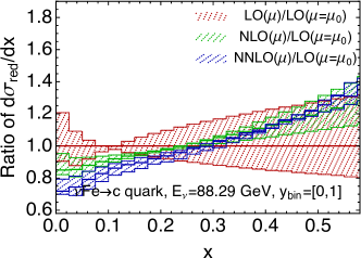
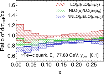
Figure 2: QCD predictions including scale variations at different orders for a differential reduced cross section in Bjorken $x$ for charm (anti-)quark production from (anti-)neutrino scattering on iron target.

In Fig. 2 we show the QCD corrections to a differential reduced cross section in Bjorken $x$ for which the electroweak couplings have been taken out. We plot the NLO and NNLO predictions normalized to the LO ones for charm (anti-)quark production from (anti-)neutrino scattering with an energy of 88.29 (77.88) GeV on iron target. The cross sections are integrated over the full range of inelasticity $y$. The hatched bands represent the scale variations as calculated by varying renormalization and factorization scale from $\mu_{F}=\mu_{R}=\mu_{0}/2$ to $2\mu_{0}$ avoiding going below the charm-quark mass. The QCD corrections are large and negative in small and moderate $x$ regions for charm quark production with the nominal scale choice. The NNLO corrections can reach about -10% for $x$ up to 0.1 and turn to positive for $x>0.4$. The scale variations at LO are large in general but vanish at $x\sim 0.1$ indicating its limitation as estimate of perturbative uncertainties. It was found even the scale variations at NLO underestimate the perturbative uncertainties at small and moderate $x$ regions due to accidental cancellations as will be explained later. The NNLO scale variations give a more reliable estimation of the perturbative uncertainties and also show improvement at high-$x$ compared with the NLO case. Results are similar for charm anti-quark production which can be related via a charge conjugate parity transformation except for the differences of initial state PDFs. Especially the charm quark production involves Cabibbo suppressed contributions at tree level from $d$-valence quark which dominate at high-$x$ while only sea-quark contributions exist for charm anti-quark production.

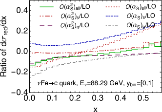
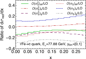
Figure 3: QCD corrections at different orders separated into partonic channels for a differential reduced cross section in Bjorken $x$ for charm (anti-)quark production from (anti-)neutrino scattering on iron target.

In the small and moderate $x$ region the NNLO corrections are almost as large as the NLO corrections. That motivates a careful examination of the convergence of the perturbative expansion. In Fig. 3 we plot the QCD corrections from two main partonic channels, i.e., with the strange (anti-)quark initial state, including Cabibbo suppressed $d$($\bar{d}$) quark contributions, and with the gluon initial state, for the same distribution as shown in Fig. 2. The right plot of Fig. 3 shows the corrections for charm anti-quark production. We observe a strong cancellation among the NLO corrections from the strange anti-quark and the gluon channels starting from small-$x$ and persisting to high-$x$ region. We regard this cancellation accidental in that it does not arise from basic principles but is a result of several factors. The cancellation of NLO corrections remains if instead using the NLO PDFs or alternative NNLO PDFs e.g., MMHT2014 Harland-Lang:2014zoa and NNPDF3.0 Ball:2014uwa . A similar cancellation has also been observed in the calculation for $t$-channel single top quark production  1404.7116 . The size of NNLO corrections are smaller than the NLO ones for the individual partonic channels indicating good convergence of the perturbative expansion. However, the cancellation between the two channels is much mild at NNLO which results in a net correction as large as the NLO one. For this reason we expect the corrections from even higher orders to be smaller than the NNLO corrections. The left plot in Fig. 3 shows results for charm quark production for which the situation is similar at low-$x$ region. At high-$x$ the correction from gluon channel flattens out due to the smaller size of gluon PDF as comparing to $d$-valence PDF, and the net correction is small and positive at NNLO.

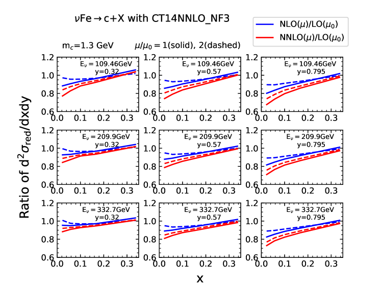
Figure 4: QCD predictions at different orders with scale choices of $\mu_{0}$ and $2\mu_{0}$ for a double differential reduced cross section in Bjorken $x$ and inelasticity $y$ for charm quark production from neutrino scattering on iron target.

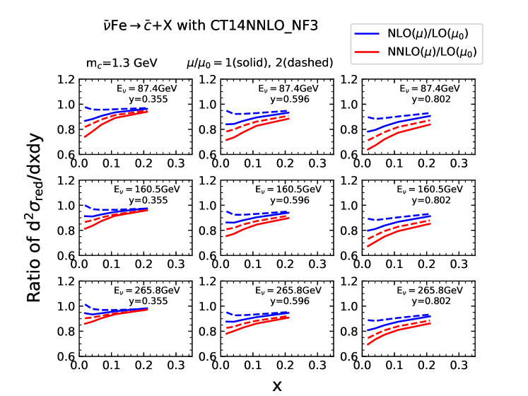
Figure 5: Similar as Fig. 4 for charm anti-quark production from anti-neutrino scattering.

We further calculate the double differential reduced cross sections in $x$ and $y$ as was measured by various experimental groups. We choose the kinematics and neutrino energies as those in CCFR Goncharov:2001qe measurement. In Fig. 4 we plot ratios of various predictions to the LO differential cross sections for charm quark production with three different energies and each with three choices of $y$. Here we use a charm-quark mass of 1.3 GeV. The solid and dotted curves correspond to using scales of $\mu_{0}$ and $2\mu_{0}$. Note the LO cross sections in the denominator are always evaluated with the scale $\mu_{0}$. For the nominal scale choice ($\mu_{0}$) the NNLO corrections are about $-10$% at $x\sim 0.02$ and a couple of percents at $x\sim 0.3$. The size of QCD corrections increases with $y$ in low-$x$ regions. Dependence on the beam energy is in the opposite direction and is weaker in general. Scale dependence of the NNLO predictions are slightly weaker than those of the NLO predictions at small-$x$. In moderate and large-$x$ regions the NLO predictions show a scale dependence that is too small due to the strong cancellations mentioned earlier. Fig. 5 shows similar results for charm anti-quark production. The QCD corrections are even more pronounced in this case due to the relatively larger gluon contributions. For $y=0.802$ the NNLO corrections can reach $-15$% for $x\sim 0.02$ and remain $-10$% for $x\sim 0.2$. The same conclusion holds for the scale dependence as in the case of charm quark production.

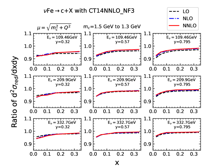
Figure 6: Dependence of a double differential reduced cross section in Bjorken $x$ and inelasticity $y$ on the charm quark mass, shown in ratios of predictions with $m_{c}=1.5$ GeV to 1.3 GeV, for charm quark production from neutrino scattering on iron target.

Since the charm quark production is usually measured at low to moderate momentum transfers, the theoretical predictions can depend significantly on the choice of charm-quark mass, in our case the pole mass. Note the determination of charm-quark pole mass has an intrinsic uncertainty of $0.1\sim 0.2$ GeV due to the renormalon ambiguity. In Fig. 6 we show the ratio of double differential cross sections calculated when using a charm-quark pole mass of 1.5 GeV to 1.3 GeV, at LO, NLO, and NNLO, for charm anti-quark production. The results for charm quark production are similar and not shown for simplicity. At LO the charm-quark mass dependence can be calculated easily. The dominant part of that is known as slow rescaling Georgi:1976vf due to the kinematic suppression, i.e., by replacing the momentum fraction in evaluation of PDFs with $\xi=x(1+m_{c}^{2}/Q^{2})$. That explains the trends we show in Fig. 6. The cross sections with larger charm-quark mass are especially suppressed in small-$x$ region and for smaller neutrino energies where the $Q^{2}$ is low. Shapes of the suppression factor with respect to $x$ are different for different values of $y$ due to the sub-dominant dependence on the mass from the hard matrix elements. The mass dependence is insensitive to higher order corrections. The NLO predictions show a slightly weaker suppression comparing to LO ones in general, especially at large-$x$ and smaller neutrino energies. Effects of NNLO corrections on the mass dependence are almost negligible for the full kinematic range considered.

2.3 Heavy quark scheme

The NNLO calculations are carried out in a fixed flavor number scheme with $n_{f}=3$. This should be the appropriate scheme for $Q\gtrsim m_{c}$. For the semiinclusive charged-current (CC) DIS process we studied, at $Q\gg m_{c}$, there exist logarithmic contributions of $\sim\alpha_{\scriptscriptstyle S}^{n}\ln^{n}(Q^{2}/m_{c}^{2})$ due to initial-state gluon splitting into a $c\bar{c}$ pair in the quasi-collinear limit. In principle that needs to be resummed by using the heavy-quark PDFs together with an appropriate general mass variable flavor number (GM-VFN) scheme, for example, the ACOT hep-ph/9312319 , FONLL 1001.2312 , or RT 1201.6180 schemes. The exact ${\mathcal{O}}(\alpha_{\scriptscriptstyle S}^{2})$ massive coefficient functions 1601.05430 complete all ingredients needed for constructing such a scheme like S-ACOT-$\chi$ Guzzi:2011ew at NNLO for the charged-current scattering. For the kinematics where the dimuon measurements carried out, the $Q^{2}$ is not too high comparing to the charm-quark mass in the bulk of the data. Besides, the experimental uncertainties are at least at the level of $5\sim 10$% for the NuTeV and CCFR measurements. Thus a VFN scheme is not of immediate relevance for the phenomenological study on dimuon measurements. We leave a formal study on the GM-VFN scheme for future publications while providing an estimate of the logarithmic contributions beyond ${\mathcal{O}}(\alpha_{\scriptscriptstyle S}^{2})$ in below.

As mentioned earlier the logarithmic contributions can be resummed effectively with a perturbative charm (anti-)quark PDF in $n_{f}=4$ scheme that follows a DGLAP evolution,

$$\frac{df^{(n_{f}=4)}_{c}(x,\mu^{2})}{d\ln\mu^{2}}=\sum_{i=q,\bar{q},c,\bar{c},g}P_{ci}(x,\alpha_{\scriptscriptstyle S}(\mu^{2}))\otimes f^{(n_{f}=4)}_{i}(x,\mu^{2}),$$ (11)

where $P_{ij}$ is the DGLAP splitting function with dependence on $n_{f}$ suppressed, $\mu$ is the factorization scale. The exact results for $P_{ij}$ are known up to three loops hep-ph/0403192 ; hep-ph/0404111 . The charm-quark PDF at arbitrary scales can be derived from the boundary conditions at $\mu=m_{c}$ by evolving upward. Note that starting at ${\mathcal{O}}(\alpha_{\scriptscriptstyle S}^{2})$ the charm-quark PDF has a small discontinuity at $\mu=m_{c}$. We can expand the charm-quark PDF in the strong coupling constant,

$$f_{c}^{(n_{f}=4)}(x,\mu^{2}) =\Delta^{(2)}+\left({\alpha_{\scriptscriptstyle S}(m_{c}^{2})\over 2\pi}\right)\left\{L(P^{(0)}_{cg}\otimes f^{(n_{f}=4)}_{g}(x,m_{c}^{2}))\right\}+\left({\alpha_{\scriptscriptstyle S}(m_{c}^{2})\over 2\pi}\right)^{2}$$

$$\Big{\{}L(\sum_{i}P^{(1)}_{ci}\otimes f^{(n_{f}=4)}_{i}(x,m_{c}^{2}))+{L^{2}\over 2}(\sum_{i}P^{(0)}_{cg}\otimes P^{(0)}_{gi}\otimes f^{(n_{f}=4)}_{i}(x,m_{c}^{2})$$

$$-\beta_{0}P^{(0)}_{cg}\otimes f^{(n_{f}=4)}_{g}(x,m_{c}^{2}))\Big{\}}+{\mathcal{O}}(\alpha_{\scriptscriptstyle S}^{3}),$$ (12)

where $\Delta^{(2)}$ is of ${\mathcal{O}}(\alpha_{\scriptscriptstyle S}^{2})$ due to the discontinuity crossing the heavy-quark threshold and $L=\ln(\mu^{2}/m^{2}_{c})$. It is understood that the strong coupling constant, the one- and two-loop splitting functions $P^{(0,1)}_{ij}$, and the one-loop $\beta$ function in Eq. (2.3) are all evaluated with $n_{f}=4$. We can translate the strong coupling constant and PDFs with $n_{f}=4$ to those with $n_{f}=3$ via matching at the charm-quark threshold hep-ph/9612398 . Furthermore, we can expand them in $\alpha_{\scriptscriptstyle S}(\mu^{2})$ instead. We arrive at an expanded solution,

$$f_{c}^{(n_{f}=4)}(x,\mu^{2}) =\Delta^{(2)}+\left({\alpha_{\scriptscriptstyle S}(\mu^{2})\over 2\pi}\right)\left\{L(P^{(0)}_{cg}\otimes f^{(n_{f}=3)}_{g}(x,\mu^{2}))\right\}+\left({\alpha_{\scriptscriptstyle S}(\mu^{2})\over 2\pi}\right)^{2}$$

$$\Big{\{}L(\sum_{i}P^{(1)}_{ci}\otimes f^{(n_{f}=3)}_{i}(x,\mu^{2}))-{L^{2}\over 2}(\sum_{i}P^{(0)}_{cg}\otimes P^{(0)}_{gi}\otimes f^{(n_{f}=3)}_{i}(x,\mu^{2})$$

$$-\beta_{0}P^{(0)}_{cg}\otimes f^{(n_{f}=3)}_{g}(x,\mu^{2}))\Big{\}}+{\mathcal{O}}(\alpha_{\scriptscriptstyle S}^{3}),$$ (13)

with $\beta$ functions and splitting functions for $n_{f}=4$. Those ${\mathcal{O}}(\alpha_{\scriptscriptstyle S})$ and ${\mathcal{O}}(\alpha_{\scriptscriptstyle S}^{2})$ logarithmic contributions have already been captured by our NLO and NNLO calculations respectively. Differences of the evolved charm-quark PDF and the expansion in Eq. (2.3) can serve as an estimate of the remaining logarithmic contributions at higher orders.

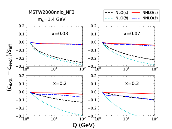
Figure 7: Differences of an evolved charm-quark PDF $c_{evol.}$ at NNLO and the expanded solution $c_{exp.}$ up to ${\mathcal{O}}(\alpha_{\scriptscriptstyle S})$ (NLO) and ${\mathcal{O}}(\alpha_{\scriptscriptstyle S}^{2})$ (NNLO) as a function of $\mu=Q$ for several $x$ values, normalized to the effective strangeness PDF $s_{eff}$. See text for more details.

In Fig. 7 we plot the differences of an evolved charm-quark PDF $c_{evol.}$ at NNLO (with 3-loop splitting functions) and the expanded solution $c_{exp.}$ up to ${\mathcal{O}}(\alpha_{\scriptscriptstyle S})$ and ${\mathcal{O}}(\alpha_{\scriptscriptstyle S}^{2})$ as a function of $\mu=Q$ for several $x$ values, normalized to the effective strangeness PDF $s_{eff}$ which is a combination of $s(\bar{s})$ and $d(\bar{d})$ PDFs. The charm quark production cross section at LO is simply proportional to the effective strangeness PDF with the slow rescaling. We use the MSTW2008 NNLO PDFs 0901.0002 with $m_{c}=$ 1.4 GeV as an input. For small $x$ values we can see the FFN calculation at ${\mathcal{O}}(\alpha_{\scriptscriptstyle S})$ misses a large portion of the logarithmic contributions that can reach 10-20% of the LO charm quark production cross sections for $Q\sim 10$ GeV. On another hand the NNLO calculation can reproduce well the resummed contributions with the remaining logarithmic contributions of about 2% of the LO cross sections for the same $Q$ values. Note the highest $Q$ value that the CCFR and NuTeV measurements probed is around 10 GeV. For large $x$ values the conclusion is similar for charm quark production. For charm anti-quark production the charm-quark PDF has a relatively larger weight due to the quick falling of the sea-quark PDFs. The contributions beyond NNLO can reach 5% for $x=0.3$ and $Q=10$ GeV.

3 Fast interface

The above calculation can not be immediately used in the global analysis of QCD due to the time-consuming nature of NNLO calculations and the fact that the analysis involves scan over a large number of PDF ensembles. Indeed even the NLO calculation is inadequate for direct use in the analysis. The PDF fitting group instead needs to rely on either K-factor approximation or fast interface based on grid interpolations. There have been quite some developments on fast interface for high-order perturbative calculations, e.g., APPLgrid Carli:2010rw , FastNLO Wobisch:2011ij , aMCfast Bertone:2014zva , starting from NLO in QCD to NNLO most recently Czakon:2017dip . We have constructed a fast interface specialized for our calculation following similar approaches. First of all the PDFs at arbitrary scales can be approximated by an interpolation on a one-dimensional grid of $x$,

$$f(x,\mu)=\sum_{i=0}^{n}f_{k+i}I_{i}^{(n)}\left(\frac{y(x)}{\delta y}-k\right),$$ (14)

where we choose the interpolation variable $y(x)=x^{0.3}$ and the interpolation order $n=4$, and $f_{j}$ is the PDF value on the $j$-th grid point. $\delta y$ has been chosen so as to give 50 grid points between $x=1$ and a minimum determined according to the specified kinematics. We use a $n$-th order polynomial interpolating function $I_{i}^{(n)}$ and the starting grid point $k$ is determined so as $x$ located in between the $(k+1)$-th and $(k+2)$-th grid points. The cross section in deep inelastic scattering can thus be expressed as

$$d\sigma_{bin}=\sum_{p}\sum_{m}\sum_{i}\left(\frac{\alpha_{s}(\mu)}{2\pi}\right)^{m}{\mathcal{B}}(p,m,i)f_{i},$$ (15)

where the summation runs over different sub-channels $p$, perturbative orders $m$, and the grid points $i$. The interpolation coefficients ${\mathcal{B}}(p,m,i)$ which are independent of the PDFs can be obtained by projecting the event weight onto the corresponding grid points during the MC integration. Once those interpolation coefficients are calculated and stored, the cross sections with any PDFs can be obtained via Eq. (15) without repeating the time-consuming calculations of the matrix elements.

In Table 1 we show the typical time cost in a direct calculation and the interpolation with the NuTeV kinematics. Also shown is the time cost for generating the interpolation grid. The direct calculation involves intensive MC integration as expected, costing about 60 CPU core-hours per data point of the double differential distribution $d^{2}\sigma/dxdy$ in charm-quark production with NuTeV kinematics. The grid generation costs four times more since it requires separation of different sub-channels. However, with the generated grid, for any PDFs the interpolation/calculation takes less than a millisecond. The precision of the interpolation are found to be around a few permille at NNLO, smaller than the typical errors from MC integration. In Fig. 8 the solid line shows the ratio of the cross sections from direct calculation and the fast interpolation using the grid generated from the same run both using CT14 NNLO PDFs, for all the data points in NuTeV and CCFR measurements with charm (anti-)quark production. In this case deviation of the two predictions are simply due to the interpolation errors. Also shown in Fig. 8 are comparison of the interpolation results for MMHT2014 and NNPDF3.0 NNLO PDFs with the grid generated from CT14, with independent direct calculations using the same PDFs. Here the two predictions for each PDF choice differ at most half percent due to the MC integration errors in the direct calculations as shown by the error bars.

	CPU core-hours (NLO)	CPU core-hours (NNLO)
direct calculation	0.5	60
grid generation	1	280
interpolation	$10^{-7}$	$10^{-7}$

Table 1: Typical time cost (in CPU core-hours) for calculation and interpolation of reduced cross section $d^{2}\sigma/dxdy$ (per data point) of charm-quark production with NuTeV kinematics.

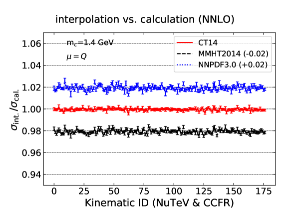
Figure 8: Ratios of the interpolated NNLO cross sections and cross sections from direct calculations using CT14, MMHT2014 and NNPDF3.0 PDFs all with the grid generated from the same run of CT14 calculation.

4 Impact on strange-quark distributions

Now we move to discuss potential impact of the NNLO calculations on constraining parton distributions, especially the strange-quark distributions, by checking the agreements of different theories with experimental data. We select the NuTeV and CCFR measurements on charm (anti-)quark production in the form of double differential cross sections $d^{2}\sigma/dxdy$, which provides dominant constraints on the strange-quark distributions, e.g., in MMHT2014 and CT14 global analyses. The theoretical predictions used in those analyses are at NLO only. We include the data point only with $Q^{2}>4\,{\rm GeV}^{2}$ to leave out the region where higher-twist corrections can be potentially large. That results in 38(33) data points for charm (anti-)quark production in NuTeV, and 40(38) data points for charm (anti-)quark production in CCFR. Besides, we have simply corrected the data for nuclear effects of iron target hep-ph/0312323 ; 1203.1290 using a parametrization of $F_{2}$ ratio measured at SLAC and NMC, instead of including more sophisticated corrections to individual parton flavors 0709.3038 ; 0902.4154 ; 1112.6324 ; 1509.00792 in the theory calculations. That leads to corrections on the data of 2% at $x\sim 0.05$, -4% at $x\sim 0.1$, and $5\%$ at $x\sim 0.4$. We did not include uncertainties on the nuclear corrections since the correction itself is already small comparing to experimental errors for the $x$ range considered. The experimental uncertainties include the total statistical and systematic errors which are treated uncorrelated among different data point. The total error for each data point has been scaled by square root of its effective freedom so as a reasonable fit should have $\chi^{2}/N_{pt}$ of one Mason:2006qa . Besides, there is an additional systematic error of 10% assumed due to the input of semi-leptonic decay branching ratio of charm quark when unfolding the dimuon cross sections back to the charm production cross sections Mason:2006qa . This normalization error is assumed to be fully correlated among all data points in both NuTeV and CCFR measurements.

In the following we first compare predictions with various PDFs to the experimental measurement. Later we show how the strange quark distributions may change if using our NNLO results instead of the NLO ones in the PDF analyses by means of Hessian profiling 1503.05221 .

4.1 Theory-data agreement with various PDFs

We considered the updated NNLO PDFs from the major PDF fitting groups, including CT14 Dulat:2015mca , MMHT14 Harland-Lang:2014zoa , NNPDF3.1 (both nominal set and set with only collider data) Ball:2017nwa , ABMP16 Alekhin:2017kpj , HERAPDF2.0 1506.06042 , and ATLAS-epWZ16 1612.03016 . For the case of NNPDF, the original PDF representation of MC replicas has been transformed into a Hessian PDF set using the MC2H package 1505.06736 . Note that we have used NNLO PDFs for both NLO and NNLO calculations. In case that the PDFs with $n_{f}=3$ are not publicly available we evolve the nominal PDFs by DGLAP evolution at 3-loop and with $n_{f}=3$ starting from a scale below the charm quark mass threshold.

We show the fits to NuTeV and CCFR data (149 data points in total) with NLO and NNLO predictions for various choices of PDFs in Table 2. Here through the calculations we have used a charm-quark pole mass of 1.3 GeV and a scale of $\mu=\sqrt{Q^{2}+m_{c}^{2}}$ despite the fact that different PDF groups use a charm-quark pole mass ranging from 1.3 to 1.6 GeV. In each fit we show the $\chi^{2}$ and the normalization shift (in unit of $1\,\sigma$ error) of the central PDFs without and with including the full PDF uncertainties. In the later case it gauges the overall agreement between data and theory with both uncertainties included. Shift with minus sign indicates the data prefer smaller values for the cross sections. Each pair of eigenvector PDFs corresponds to one correlated theoretical error with symmetric Gaussian distribution when including the PDF uncertainties 1503.05221 . For the HERA and ATLAS fits the PDF uncertainties include those model and parametrization uncertainties as well. Note the $\chi^{2}$ shown here may not represent the actual fit quality of the same data in their global analyses since there different predictions or input parameters are used.

$N_{pt}=149$	NLO		NNLO
CT14	167.3(-1.0)	130.2(1.1)	154.2(-0.4)	132.9(1.3)
MMHT14	132.2(-1.0)	118.6(0.1)	127.7(-0.3)	118.8(0.1)
NNPDF3.1	157.8(-1.2)	115.8(-1.0)	161.3(-0.5)	115.1(-0.6)
ABMP16	189.3(-1.6)	170.8(-0.8)	170.2(-1.0)	157.6(-0.3)
HERAPDF2.0	258.4(-0.8)	130.3(0.3)	221.6(-0.1)	132.0(0.5)
ATLAS-epWZ16	352.8(-4.0)	246.6(-2.1)	321.5(-3.7)	228.7(-1.6)
NNPDF3.1 (collider)	513.4(-5.1)	118.5(-2.3)	537.8(-4.8)	114.0(-1.9)

Table 2: $\chi^{2}$ and normalization shift (in unit of $1\,\sigma$ error) of fits to NuTeV and CCFR charm production data with various theoretical predictions using $m_{c}=1.3$ GeV and $\mu=\sqrt{Q^{2}+m_{c}^{2}}$. The shifts are shown in brackets with minus sign indicating the data prefer smaller values for the cross sections. The numbers in bold font correspond to fits including the full PDF uncertainties as well.

The PDFs shown in Table 2 fall into two distinct groups, those without including any dimuon data in the PDF analysis, namely the HERA, ATLAS, and NNPDF collider-only PDFs, and the others with dimuon data, either from NuTeV, CCFR, CHORUS, or NOMAD. The $\chi^{2}/N_{pt}$ are about one for PDFs in the second group as all the dimuon data consistently prefer a suppressed strangeness as discussed in the introduction section. Interestingly, CT14, MMHT14 and NNPDF3.1 show very similar results on $\chi^{2}$ and also the normalization shift. The NNLO predictions without PDF uncertainties give slightly smaller $\chi^{2}$ in general for the specified mass and scale as comparing to NLO, though those PDFs are fitted with NLO or approximate NNLO predictions. For PDFs from collider-only data, the fits are rather poor if not taking into account the PDF uncertainties. One reason is the ATLAS W/Z data do prefer larger central values of the strange-quark PDFs. With the PDF uncertainties included, the $\chi^{2}/N_{pt}$ have been reduced to below one for HERA and NNPDF collider-only PDFs indicating consistency of their PDFs and the dimuon data once both uncertainties are considered. The situation is different for the ATLAS PDFs where $\chi^{2}/N_{pt}$ is still about 1.5 even for the NNLO predictions. That can be further visualized by a direct comparison of theory and data as in Figs. 9 and 10 for NuTeV charm quark and anti-quark production respectively. Most of the data points lie far outside the PDF error bands with a non-trivial shape dependence. The PDF uncertainties of charm quark cross sections are smaller than the ones of charm anti-quark in general since the former also involves contribution from $d$ valence quark which is better constrained than sea quarks. We conclude the ATLAS PDFs can not describe the dimuon data well and the NNLO calculations can only bring in limited improvement.

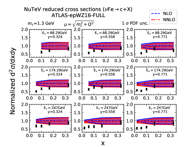
Figure 9: NLO and NNLO predictions on charm quark production cross sections using ATLAS-epWZ16 NNLO PDFs comparing with the NuTeV measurement. Also shown are the 1 $\sigma$ PDF uncertainties. The experimental data have been corrected for nuclear effects. The error bars represent the total experimental uncertainties rescaled by square root of the effective degree of freedoms. A 10% normalization uncertainty due to the semi-leptonic decay BR of charm quark is not shown here.

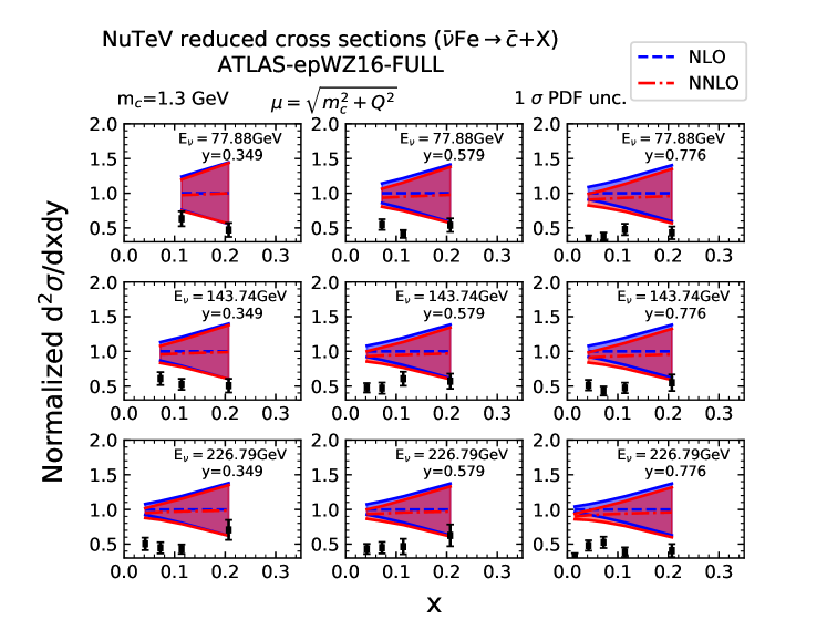
Figure 10: Similar as Fig. 9 for charm anti-quark production using ATLAS-epWZ16 NNLO PDFs.

We further compare predictions from the same PDF sets but with different scale and charm quark mass inputs as shown in Tables 3 and 4. From Table 3 we can see that by using a scale of twice of the nominal choice the agreement between NLO predictions and data deteriorates, especially in the case of without PDF uncertainties. In comparison the $\chi^{2}$ for NNLO predictions are less sensitive to the change of scale for both with and without PDF uncertainties. The cross sections are reduced especially at small-$x$ when using a larger charm-quark mass of 1.4 GeV as shown already in Fig. 6. As show in Table 4 that leads to a smaller $\chi^{2}$ at NLO in general comparing with Table 2 when no PDF uncertainties are included. At NNLO the $\chi^{2}$ can either decrease or increase depending on the PDFs considered indicating a different preference of charm-quark mass at NNLO comparing with NLO for certain PDFs. The $\chi^{2}$ for the ATLAS PDFs are reduces as well. However, in both cases the $\chi^{2}$ are still over 200 for predictions with the ATLAS PDFs.

$N_{pt}=149$	NLO		NNLO
CT14	196.1(-1.3)	131.6(1.2)	160.3(-0.7)	130.5(1.3)
MMHT14	152.7(-1.3)	123.1(0.0)	127.1(-0.6)	117.7(0.2)
NNPDF3.1	163.1(-1.5)	119.2(-1.2)	153.2(-0.8)	114.4(-0.7)
ABMP16	223.5(-1.8)	197.1(-1.1)	180.6(-1.3)	161.8(-0.6)
HERAPDF2.0	308.4(-1.2)	130.3(0.5)	238.9(-0.5)	130.2(0.5)
ATLAS-epWZ16	391.5(-4.1)	271.4(-2.4)	339.7(-3.8)	239.4(-1.8)
NNPDF3.1 (collider)	487.7(-5.1)	124.1(-2.6)	521.0(-5.0)	116.4(-2.0)

Table 3: Similar as Table 2 but with $\mu=2\sqrt{Q^{2}+m_{c}^{2}}$.

$N_{pt}=149$	NLO		NNLO
CT14	158.2(-0.8)	131.1(1.0)	150.5(-0.1)	134.1(1.3)
MMHT14	128.2(-0.8)	118.9(0.0)	129.4(-0.1)	119.6(0.1)
NNPDF3.1	156.6(-1.0)	115.9(-0.9)	166.4(-0.3)	115.5(-0.5)
ABMP16	177.1(-1.4)	162.6(-0.7)	163.2(-0.8)	153.2(-0.1)
HERAPDF2.0	240.9(-0.6)	130.5(0.2)	209.2(0.2)	132.6(0.5)
ATLAS-epWZ16	332.8(-3.9)	234.4(-2.0)	303.5(-3.5)	218.9(-1.5)
NNPDF3.1 (collider)	527.0(-5.0)	116.4(-2.2)	553.7(-4.8)	110.2(-1.9)

Table 4: Similar as Table 2 but with $m_{c}=1.4$ GeV and $\mu=Q$.

4.2 Hessian profiling of PDFs

One main motivation of this paper is to investigate impact of the NNLO calculations on extraction of the strange quark PDFs in global analyses including the dimuon data. Precisely we would like to see how the outcome strange quark PDFs change when using NNLO predictions instead of the NLO ones, as only NLO predictions are available in previous PDF fits. That could be done by individual PDF groups using the fast interface and grids presented in this paper. Alternatively we can estimate the possible shift of the PDFs by means of Hessian profiling 1503.05221 . In Hessian profiling the PDF parameters are assumed to follow a prior multi-Gaussian distribution. That corresponds effectively to a parabolic shape of the prior $\chi^{2}$ around the central PDF and with $\Delta\chi^{2}=1$ when reaching the $1\,\sigma$ error in each eigenvector direction. The $\chi^{2}$ of any new data set to be included also forms a parabola in the PDF parameter space under linear approximation. The profiled PDFs are thus determined according to profiles of the total $\chi^{2}$, e.g., by minimization of the total $\chi^{2}$ for the central value and $\Delta\chi^{2}=1$ for the PDF uncertainties. We stress here the Hessian profiling can only serve as an estimation of the effects of new data or theory on the PDFs since an actual PDF fit involves further complexities due to e.g., parametrization dependence and the requirement of tolerance conditions.

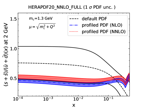
Figure 11: PDF ratio of strange to non-strange sea-quarks at 2 GeV as a function of $x$ for the HERAPDF2.0 NNLO PDFs. The solid black lines indicate the upper/lower uncertainties of original PDFs. The colored bands represent the central value and uncertainty after profiling using the NuTeV and CCFR charm (anti-)quark production data with the NLO and NNLO predictions.

We start with the HERAPDF2.0 NNLO PDFs which does not include any dimuon data but rather implements certain model constraints on the strangeness fraction and shape. We show the PDF ratio of strange to non-strange sea-quarks, $R_{s}$ at a scale of 2 GeV in Fig. 11. We can see a moderate suppression of the strangeness in small to intermediate $x$ region comparing to the $u$ and $d$ sea-quarks and a rapid falloff at large $x$. The PDF uncertainties as indicated by the solid black lines are large, more than 30% in the entire $x$ range, which include the experimental, model, and parametrization uncertainties. The colored bands in Fig. 11 are for the profiled PDFs with the NuTeV and CCFR charm (anti-)quark production data together using the NLO and NNLO theoretical predictions. It is clear that the dimuon data prefers an even suppressed strangeness with $R_{s}$ of about 0.5 in the full range of $x$. The profiled PDFs lie at the lower edge of the $1\,\sigma$ error of the original PDFs indicating reasonable agreement between original PDFs and the dimuon data as already seen in Table 2. The profiled PDFs have a much smaller uncertainties on $R_{s}$ than the original PDFs as one expect. We notice that the PDF uncertainties are also reduced significantly in the small $x$ region $10^{-4}-10^{-2}$ which are beyond the coverage of the dimuon data. That is possibly due to the restricted parametrization form of strange quark PDFs used in the HERA PDF analysis. Importantly we found the NNLO predictions prefer higher values of $R_{s}$ than the NLO ones, in this case well above the $1\,\sigma$ error band of the later. That can be understood since the NNLO corrections are negative in the bulk of the data.

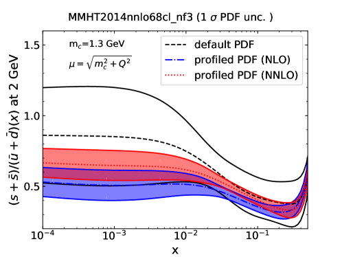
Figure 12: Similar as Fig. 11 for profiling of the MMHT2014 NNLO PDFs.

We perform another profiling study with the MMHT2014 NNLO PDFs as shown in Fig. 12. Noted that since the MMHT2014 analysis already includes above dimuon data, the study here only means for checking impact of the NNLO corrections. We can see the NNLO predictions prefer larger strangeness than NLO predictions for $x$ up to a few times 0.1 and by a similar amount as in Fig. 11. The shift of central values of the NLO profiled PDFs comparing to the original PDFs, though still within the PDF error band, is due to several facts. In the MMHT2014 fits Harland-Lang:2014zoa they use a charm-quark pole mass of 1.4 GeV and a semi-leptonic decay branching ratio of charm quark that is 7% lower than the one extracted by NuTeV and CCFR, both of which lead to an increase of the strange-quark PDFs. Besides, there are also LHC data in the MMHT analysis that pull the ratio further up. The uncertainties are largely reduced in the profiled PDFs mostly because we use the $\Delta\chi^{2}=1$ criterion rather than a dynamic tolerance condition as in the MMHT analysis. We have also compared the profiled PDFs with alternative scale choices and found those with NNLO predictions are less sensitive to the choice of scale.

5 Conclusion

In conclusion we have presented details on calculation of next-to-next-to-leading order QCD corrections to massive charged-current coefficient functions in deep-inelastic scattering. We focus on the application to charm-quark production in neutrino scattering on fixed target that can be measured via the dimuon final state as in the NuTeV and CCFR experiments. We construct a fast interface to the calculation so for any parton distributions the dimuon cross sections can be evaluated within milliseconds by using the pre-generated interpolation grids. The NNLO predictions thus can be conveniently included in future global analyses of QCD involving the dimuon data. We further compare the dimuon data with the NNLO predictions using various PDFs and confirm the pull of the ATLAS data on the strange-quark PDFs. Moreover, we study impact of the NNLO corrections on the extraction of strange-quark PDFs in the context of Hessian profiling, and find with the NNLO predictions the dimuon data tend to favor larger strange-quark PDFs than with the NLO predictions. The fast interface together with the interpolation grids for dimuon cross sections are publicly available upon request. A definite conclusion on the potential inconsistency of the DIS and ATLAS data awaits the ongoing global fits by the PDF analysis groups.

- (1) ZEUS, H1 Collaboration, H. Abramowicz et al., Combination of measurements of inclusive deep inelastic scattering cross sections and QCD analysis of HERA data, Eur. Phys. J. C75 (2015), no. 12 580, [arXiv:1506.06042].
- (2) J. Gao, L. Harland-Lang, and J. Rojo, The Structure of the Proton in the LHC Precision Era, arXiv:1709.04922.
- (3) E. Laenen, S. Riemersma, J. Smith, and W. L. van Neerven, Complete O (alpha-s) corrections to heavy flavor structure functions in electroproduction, Nucl. Phys. B392 (1993) 162–228.
- (4) E. Laenen, S. Riemersma, J. Smith, and W. L. van Neerven, O(alpha-s) corrections to heavy flavor inclusive distributions in electroproduction, Nucl. Phys. B392 (1993) 229–250.
- (5) T. Gottschalk, Chromodynamic Corrections to Neutrino Production of Heavy Quarks, Phys. Rev. D23 (1981) 56.
- (6) M. Gluck, S. Kretzer, and E. Reya, Detailed next-to-leading order analysis of deep inelastic neutrino induced charm production off strange sea partons, Phys. Lett. B398 (1997) 381–386, [hep-ph/9701364]. [Erratum: Phys. Lett.B405,392(1997)].
- (7) J. Blumlein, A. Hasselhuhn, P. Kovacikova, and S. Moch, Heavy Flavor Corrections to Charged Current Deep-Inelastic Scattering in Mellin Space, Phys. Lett. B700 (2011) 294–304, [arXiv:1104.3449].
- (8) S. Alekhin, J. Blumlein, L. Caminadac, K. Lipka, K. Lohwasser, S. Moch, R. Petti, and R. Placakyte, Determination of Strange Sea Quark Distributions from Fixed-target and Collider Data, Phys. Rev. D91 (2015), no. 9 094002, [arXiv:1404.6469].
- (9) E. L. Berger, J. Gao, C. S. Li, Z. L. Liu, and H. X. Zhu, Charm-Quark Production in Deep-Inelastic Neutrino Scattering at Next-to-Next-to-Leading Order in QCD, Phys. Rev. Lett. 116 (2016), no. 21 212002, [arXiv:1601.05430].
- (10) A. Behring, J. Blümlein, A. De Freitas, A. Hasselhuhn, A. von Manteuffel, and C. Schneider, O() heavy flavor contributions to the charged current structure function at large momentum transfer, Phys. Rev. D92 (2015), no. 11 114005, [arXiv:1508.01449].
- (11) NuTeV Collaboration, M. Goncharov et al., Precise measurement of dimuon production cross-sections in muon neutrino Fe and muon anti-neutrino Fe deep inelastic scattering at the Tevatron, Phys. Rev. D64 (2001) 112006, [hep-ex/0102049].
- (12) D. A. Mason, Measurement of the strange - antistrange asymmetry at NLO in QCD from NuTeV dimuon data. PhD thesis, Oregon U., 2006.
- (13) CHORUS Collaboration, A. Kayis-Topaksu et al., Leading order analysis of neutrino induced dimuon events in the CHORUS experiment, Nucl. Phys. B798 (2008) 1–16, [arXiv:0804.1869].
- (14) NOMAD Collaboration, O. Samoylov et al., A Precision Measurement of Charm Dimuon Production in Neutrino Interactions from the NOMAD Experiment, Nucl. Phys. B876 (2013) 339–375, [arXiv:1308.4750].
- (15) S. Dulat, T.-J. Hou, J. Gao, M. Guzzi, J. Huston, P. Nadolsky, J. Pumplin, C. Schmidt, D. Stump, and C. P. Yuan, New parton distribution functions from a global analysis of quantum chromodynamics, Phys. Rev. D93 (2016), no. 3 033006, [arXiv:1506.07443].
- (16) L. A. Harland-Lang, A. D. Martin, P. Motylinski, and R. S. Thorne, Parton distributions in the LHC era: MMHT 2014 PDFs, Eur. Phys. J. C75 (2015), no. 5 204, [arXiv:1412.3989].
- (17) NNPDF Collaboration, R. D. Ball et al., Parton distributions from high-precision collider data, arXiv:1706.00428.
- (18) F. Carvalho, F. O. Duraes, F. S. Navarra, M. Nielsen, and F. M. Steffens, Meson cloud and SU(3) symmetry breaking in parton distributions, Eur. Phys. J. C18 (2000) 127–136, [hep-ph/9912378].
- (19) R. Vogt, Physics of the nucleon sea quark distributions, Prog. Part. Nucl. Phys. 45 (2000) S105–S169, [hep-ph/0011298].
- (20) H. Chen, F. G. Cao, and A. I. Signal, Strange sea distributions of the nucleon, J. Phys. G37 (2010) 105006, [arXiv:0912.0351].
- (21) P. M. Nadolsky, H.-L. Lai, Q.-H. Cao, J. Huston, J. Pumplin, D. Stump, W.-K. Tung, and C. P. Yuan, Implications of CTEQ global analysis for collider observables, Phys. Rev. D78 (2008) 013004, [arXiv:0802.0007].
- (22) A. Kusina, T. Stavreva, S. Berge, F. I. Olness, I. Schienbein, K. Kovarik, T. Jezo, J. Y. Yu, and K. Park, Strange Quark PDFs and Implications for Drell-Yan Boson Production at the LHC, Phys. Rev. D85 (2012) 094028, [arXiv:1203.1290].
- (23) M. W. Krasny, F. Dydak, F. Fayette, W. Placzek, and A. Siodmok, at the LHC: a forlorn hope?, Eur. Phys. J. C69 (2010) 379–397, [arXiv:1004.2597].
- (24) G. Bozzi, J. Rojo, and A. Vicini, The Impact of PDF uncertainties on the measurement of the W boson mass at the Tevatron and the LHC, Phys. Rev. D83 (2011) 113008, [arXiv:1104.2056].
- (25) M. Baak et al., Working Group Report: Precision Study of Electroweak Interactions, in Proceedings, 2013 Community Summer Study on the Future of U.S. Particle Physics: Snowmass on the Mississippi (CSS2013): Minneapolis, MN, USA, July 29-August 6, 2013, 2013. arXiv:1310.6708.
- (26) ATLAS Collaboration, M. Aaboud et al., Precision measurement and interpretation of inclusive , and production cross sections with the ATLAS detector, Eur. Phys. J. C77 (2017), no. 6 367, [arXiv:1612.03016].
- (27) ATLAS Collaboration, G. Aad et al., Determination of the strange quark density of the proton from ATLAS measurements of the and cross sections, Phys. Rev. Lett. 109 (2012) 012001, [arXiv:1203.4051].
- (28) S. Alekhin, J. Blümlein, S. Moch, and R. Placakyte, Parton distribution functions, , and heavy-quark masses for LHC Run II, Phys. Rev. D96 (2017), no. 1 014011, [arXiv:1701.05838].
- (29) S. Alekhin, J. Blümlein, and S. Moch, Strange sea determination from collider data, arXiv:1708.01067.
- (30) S. Catani and M. Grazzini, An NNLO subtraction formalism in hadron collisions and its application to Higgs boson production at the LHC, Phys. Rev. Lett. 98 (2007) 222002, [hep-ph/0703012].
- (31) J. Gao, C. S. Li, and H. X. Zhu, Top Quark Decay at Next-to-Next-to Leading Order in QCD, Phys. Rev. Lett. 110 (2013), no. 4 042001, [arXiv:1210.2808].
- (32) J. Gao and H. X. Zhu, Electroweak prodution of top-quark pairs in e+e- annihilation at NNLO in QCD: the vector contributions, Phys. Rev. D90 (2014), no. 11 114022, [arXiv:1408.5150].
- (33) J. Gao and H. X. Zhu, Top Quark Forward-Backward Asymmetry in Annihilation at Next-to-Next-to-Leading Order in QCD, Phys. Rev. Lett. 113 (2014), no. 26 262001, [arXiv:1410.3165].
- (34) R. Boughezal, C. Focke, X. Liu, and F. Petriello, -boson production in association with a jet at next-to-next-to-leading order in perturbative QCD, Phys. Rev. Lett. 115 (2015), no. 6 062002, [arXiv:1504.02131].
- (35) J. Gaunt, M. Stahlhofen, F. J. Tackmann, and J. R. Walsh, N-jettiness Subtractions for NNLO QCD Calculations, JHEP 09 (2015) 058, [arXiv:1505.04794].
- (36) E. L. Berger, J. Gao, C. P. Yuan, and H. X. Zhu, NNLO QCD Corrections to t-channel Single Top-Quark Production and Decay, Phys. Rev. D94 (2016), no. 7 071501, [arXiv:1606.08463].
- (37) H. T. Li and J. Wang, Fully Differential Higgs Pair Production in Association With a Boson at Next-to-Next-to-Leading Order in QCD, Phys. Lett. B765 (2017) 265–271, [arXiv:1607.06382].
- (38) E. L. Berger, J. Gao, and H. X. Zhu, Differential Distributions for t-channel Single Top-Quark Production and Decay at Next-to-Next-to-Leading Order in QCD, arXiv:1708.09405.
- (39) H. T. Li, C. S. Li, and J. Wang, Fully Differential Higgs Pair Production in Association With a Boson at Next-to-Next-to-Leading Order in QCD, arXiv:1710.02464.
- (40) C. W. Bauer, S. Fleming, and M. E. Luke, Summing Sudakov logarithms in B X(s gamma) in effective field theory, Phys. Rev. D63 (2000) 014006, [hep-ph/0005275].
- (41) C. W. Bauer, S. Fleming, D. Pirjol, and I. W. Stewart, An Effective field theory for collinear and soft gluons: Heavy to light decays, Phys. Rev. D63 (2001) 114020, [hep-ph/0011336].
- (42) C. W. Bauer, D. Pirjol, and I. W. Stewart, Soft collinear factorization in effective field theory, Phys. Rev. D65 (2002) 054022, [hep-ph/0109045].
- (43) C. W. Bauer, S. Fleming, D. Pirjol, I. Z. Rothstein, and I. W. Stewart, Hard scattering factorization from effective field theory, Phys. Rev. D66 (2002) 014017, [hep-ph/0202088].
- (44) M. Czakon, A novel subtraction scheme for double-real radiation at NNLO, Phys. Lett. B693 (2010) 259–268, [arXiv:1005.0274].
- (45) R. Boughezal, K. Melnikov, and F. Petriello, A subtraction scheme for NNLO computations, Phys. Rev. D85 (2012) 034025, [arXiv:1111.7041].
- (46) T. Binoth and G. Heinrich, Numerical evaluation of phase space integrals by sector decomposition, Nucl. Phys. B693 (2004) 134–148, [hep-ph/0402265].
- (47) C. Anastasiou, K. Melnikov, and F. Petriello, A new method for real radiation at NNLO, Phys. Rev. D69 (2004) 076010, [hep-ph/0311311].
- (48) A. Gehrmann-De Ridder, T. Gehrmann, and E. W. N. Glover, Antenna subtraction at NNLO, JHEP 09 (2005) 056, [hep-ph/0505111].
- (49) J. Currie, E. W. N. Glover, and S. Wells, Infrared Structure at NNLO Using Antenna Subtraction, JHEP 04 (2013) 066, [arXiv:1301.4693].
- (50) V. Del Duca, C. Duhr, G. Somogyi, F. Tramontano, and Z. Trócsányi, Higgs boson decay into b-quarks at NNLO accuracy, JHEP 04 (2015) 036, [arXiv:1501.07226].
- (51) M. Cacciari, F. A. Dreyer, A. Karlberg, G. P. Salam, and G. Zanderighi, Fully Differential Vector-Boson-Fusion Higgs Production at Next-to-Next-to-Leading Order, Phys. Rev. Lett. 115 (2015), no. 8 082002, [arXiv:1506.02660].
- (52) I. W. Stewart, F. J. Tackmann, and W. J. Waalewijn, Factorization at the LHC: From PDFs to Initial State Jets, Phys. Rev. D81 (2010) 094035, [arXiv:0910.0467].
- (53) I. W. Stewart, F. J. Tackmann, and W. J. Waalewijn, N-Jettiness: An Inclusive Event Shape to Veto Jets, Phys. Rev. Lett. 105 (2010) 092002, [arXiv:1004.2489].
- (54) R. Bonciani and A. Ferroglia, Two-Loop QCD Corrections to the Heavy-to-Light Quark Decay, JHEP 11 (2008) 065, [arXiv:0809.4687].
- (55) H. M. Asatrian, C. Greub, and B. D. Pecjak, NNLO corrections to anti-B X(u) l anti-nu in the shape-function region, Phys. Rev. D78 (2008) 114028, [arXiv:0810.0987].
- (56) M. Beneke, T. Huber, and X. Q. Li, Two-loop QCD correction to differential semi-leptonic b u decays in the shape-function region, Nucl. Phys. B811 (2009) 77–97, [arXiv:0810.1230].
- (57) G. Bell, NNLO corrections to inclusive semileptonic B decays in the shape-function region, Nucl. Phys. B812 (2009) 264–289, [arXiv:0810.5695].
- (58) T. Becher and M. Neubert, Toward a NNLO calculation of the anti-B X(s) gamma decay rate with a cut on photon energy: I. Two-loop result for the soft function, Phys. Lett. B633 (2006) 739–747, [hep-ph/0512208].
- (59) J. R. Gaunt, M. Stahlhofen, and F. J. Tackmann, The Quark Beam Function at Two Loops, JHEP 04 (2014) 113, [arXiv:1401.5478].
- (60) I. Moult, L. Rothen, I. W. Stewart, F. J. Tackmann, and H. X. Zhu, Subleading Power Corrections for N-Jettiness Subtractions, Phys. Rev. D95 (2017), no. 7 074023, [arXiv:1612.00450].
- (61) R. Boughezal, X. Liu, and F. Petriello, Power Corrections in the N-jettiness Subtraction Scheme, JHEP 03 (2017) 160, [arXiv:1612.02911].
- (62) S. Catani and M. H. Seymour, A General algorithm for calculating jet cross-sections in NLO QCD, Nucl. Phys. B485 (1997) 291–419, [hep-ph/9605323]. [Erratum: Nucl. Phys.B510,503(1998)].
- (63) S. Catani, S. Dittmaier, M. H. Seymour, and Z. Trocsanyi, The Dipole formalism for next-to-leading order QCD calculations with massive partons, Nucl. Phys. B627 (2002) 189–265, [hep-ph/0201036].
- (64) J. M. Campbell and F. Tramontano, Next-to-leading order corrections to Wt production and decay, Nucl. Phys. B726 (2005) 109–130, [hep-ph/0506289].
- (65) H. Murayama, I. Watanabe, and K. Hagiwara, HELAS: HELicity amplitude subroutines for Feynman diagram evaluations, .
- (66) G. Cullen et al., GS-2.0: a tool for automated one-loop calculations within the Standard Model and beyond, Eur. Phys. J. C74 (2014), no. 8 3001, [arXiv:1404.7096].
- (67) T. Gleisberg, S. Hoeche, F. Krauss, M. Schonherr, S. Schumann, F. Siegert, and J. Winter, Event generation with SHERPA 1.1, JHEP 02 (2009) 007, [arXiv:0811.4622].
- (68) Particle Data Group Collaboration, J. Beringer et al., Review of Particle Physics (RPP), Phys. Rev. D86 (2012) 010001.
- (69) NNPDF Collaboration, R. D. Ball et al., Parton distributions for the LHC Run II, JHEP 04 (2015) 040, [arXiv:1410.8849].
- (70) M. Brucherseifer, F. Caola, and K. Melnikov, On the NNLO QCD corrections to single-top production at the LHC, Phys. Lett. B736 (2014) 58–63, [arXiv:1404.7116].
- (71) H. Georgi and H. D. Politzer, Precocious Scaling, Rescaling and xi Scaling, Phys. Rev. Lett. 36 (1976) 1281. [Erratum: Phys. Rev. Lett.37,68(1976)].
- (72) M. A. G. Aivazis, J. C. Collins, F. I. Olness, and W.-K. Tung, Leptoproduction of heavy quarks. 2. A Unified QCD formulation of charged and neutral current processes from fixed target to collider energies, Phys. Rev. D50 (1994) 3102–3118, [hep-ph/9312319].
- (73) S. Forte, E. Laenen, P. Nason, and J. Rojo, Heavy quarks in deep-inelastic scattering, Nucl. Phys. B834 (2010) 116–162, [arXiv:1001.2312].
- (74) R. S. Thorne, Effect of changes of variable flavor number scheme on parton distribution functions and predicted cross sections, Phys. Rev. D86 (2012) 074017, [arXiv:1201.6180].
- (75) M. Guzzi, P. M. Nadolsky, H.-L. Lai, and C. P. Yuan, General-Mass Treatment for Deep Inelastic Scattering at Two-Loop Accuracy, Phys. Rev. D86 (2012) 053005, [arXiv:1108.5112].
- (76) S. Moch, J. A. M. Vermaseren, and A. Vogt, The Three loop splitting functions in QCD: The Nonsinglet case, Nucl. Phys. B688 (2004) 101–134, [hep-ph/0403192].
- (77) A. Vogt, S. Moch, and J. A. M. Vermaseren, The Three-loop splitting functions in QCD: The Singlet case, Nucl. Phys. B691 (2004) 129–181, [hep-ph/0404111].
- (78) M. Buza, Y. Matiounine, J. Smith, and W. L. van Neerven, Charm electroproduction viewed in the variable flavor number scheme versus fixed order perturbation theory, Eur. Phys. J. C1 (1998) 301–320, [hep-ph/9612398].
- (79) A. D. Martin, W. J. Stirling, R. S. Thorne, and G. Watt, Parton distributions for the LHC, Eur. Phys. J. C63 (2009) 189–285, [arXiv:0901.0002].
- (80) T. Carli, D. Clements, A. Cooper-Sarkar, C. Gwenlan, G. P. Salam, F. Siegert, P. Starovoitov, and M. Sutton, A posteriori inclusion of parton density functions in NLO QCD final-state calculations at hadron colliders: The APPLGRID Project, Eur. Phys. J. C66 (2010) 503–524, [arXiv:0911.2985].
- (81) fastNLO Collaboration, M. Wobisch, D. Britzger, T. Kluge, K. Rabbertz, and F. Stober, Theory-Data Comparisons for Jet Measurements in Hadron-Induced Processes, arXiv:1109.1310.
- (82) V. Bertone, R. Frederix, S. Frixione, J. Rojo, and M. Sutton, aMCfast: automation of fast NLO computations for PDF fits, JHEP 08 (2014) 166, [arXiv:1406.7693].
- (83) M. Czakon, D. Heymes, and A. Mitov, fastNLO tables for NNLO top-quark pair differential distributions, arXiv:1704.08551.
- (84) F. Olness, J. Pumplin, D. Stump, J. Huston, P. M. Nadolsky, H. L. Lai, S. Kretzer, J. F. Owens, and W. K. Tung, Neutrino dimuon production and the strangeness asymmetry of the nucleon, Eur. Phys. J. C40 (2005) 145–156, [hep-ph/0312323].
- (85) M. Hirai, S. Kumano, and T. H. Nagai, Determination of nuclear parton distribution functions and their uncertainties in next-to-leading order, Phys. Rev. C76 (2007) 065207, [arXiv:0709.3038].
- (86) K. J. Eskola, H. Paukkunen, and C. A. Salgado, EPS09: A New Generation of NLO and LO Nuclear Parton Distribution Functions, JHEP 04 (2009) 065, [arXiv:0902.4154].
- (87) D. de Florian, R. Sassot, P. Zurita, and M. Stratmann, Global Analysis of Nuclear Parton Distributions, Phys. Rev. D85 (2012) 074028, [arXiv:1112.6324].
- (88) K. Kovarik et al., nCTEQ15 - Global analysis of nuclear parton distributions with uncertainties in the CTEQ framework, Phys. Rev. D93 (2016), no. 8 085037, [arXiv:1509.00792].
- (89) HERAFitter developers’ Team Collaboration, S. Camarda et al., QCD analysis of - and -boson production at Tevatron, Eur. Phys. J. C75 (2015), no. 9 458, [arXiv:1503.05221].
- (90) S. Alekhin, J. Blümlein, S. Moch, and R. Placakyte, Parton distribution functions, , and heavy-quark masses for LHC Run II, Phys. Rev. D96 (2017), no. 1 014011, [arXiv:1701.05838].
- (91) S. Carrazza, S. Forte, Z. Kassabov, J. I. Latorre, and J. Rojo, An Unbiased Hessian Representation for Monte Carlo PDFs, Eur. Phys. J. C75 (2015), no. 8 369, [arXiv:1505.06736].