The impact of star formation histories on stellar mass estimation: implications from the Local Group dwarf galaxies

Abstract

Local Group (LG) galaxies have relatively accurate star formation histories (SFHs) and metallicity evolution derived from resolved color-magnitude diagram (CMD) modeling, and thus offer a unique opportunity to explore the efficacy of estimating stellar mass $\mathcal{M_{\star}}$ of real galaxies based on the integrated stellar luminosities. Building on the SFHs and metallicity evolution of 40 LG dwarf galaxies, we carried out a comprehensive study of the influence of SFHs, metallicity evolution, and dust extinction on the UV-to-NIR color–mass-to-light-ratio (color–$\log\Upsilon_{\star}$($\lambda$)) distributions and $\mathcal{M_{\star}}$ estimation of local universe galaxies. We find that: 1) The LG galaxies follow color–$\log\Upsilon_{\star}$($\lambda$) relations that fall in between the ones calibrated by previous studies; 2) Optical color–$\log\Upsilon_{\star}$($\lambda$) relations at higher [M/H] are generally broader and steeper; 3) The SFH shape parameter “concentration” does not significantly affect the color–$\log\Upsilon_{\star}$($\lambda$) relations; 4) Light-weighted ages $\langle{\rm age}\rangle_{\rm\lambda}$ and metallicities $\langle{\rm[M/H]}\rangle_{\rm\lambda}$ of galaxies are the closest analogs to ages and metallicities of single stellar populations, and the two together constrain $\log\Upsilon_{\star}$($\lambda$) with uncertainties ranging from $\lesssim$ 0.1 dex for the NIR up to 0.2 dex for the optical passbands; 5) Metallicity evolution induces significant uncertainties to the optical but not NIR $\Upsilon_{\star}$($\lambda$) at given $\langle{\rm age}\rangle_{\rm\lambda}$ and $\langle{\rm[M/H]}\rangle_{\rm\lambda}$; 6) The $V$ band is the ideal luminance passband for estimating $\Upsilon_{\star}$($\lambda$) from single colors, because the combinations of $\Upsilon_{\star}$($V$) and optical colors such as $B$$-$$V$ and $g$$-$$r$ exhibit the weakest systematic dependences on SFHs, metallicities and dust extinction; 7) Without any prior assumption on SFHs, $\mathcal{M_{\star}}$ is constrained with biases $\lesssim$ 0.3 dex by the UV- or optical-to-NIR SED fitting. Optical passbands alone constrain $\mathcal{M_{\star}}$ with biases $\lesssim$ 0.4 dex (or $\lesssim$ 0.6 dex) when dust extinction is fixed (or variable) in SED fitting. SED fitting with monometallic SFH models tends to underestimate $\mathcal{M_{\star}}$ of real galaxies. $\mathcal{M_{\star}}$ tends to be overestimated (or underestimated) at the youngest (or oldest) $\langle{\rm age}\rangle_{\rm mass}$.

I. Introduction

Stellar mass is among the most fundamental properties of a galaxy, and it traces the galaxy formation and evolution. Stellar masses of galaxies are typically estimated from the integrated stellar luminosities by adopting appropriate stellar mass-to-light ratios, $\Upsilon_{\star}$, which in turn depend on the stellar initial mass function (IMF), stellar evolution/atmosphere models, dust extinction, star formation histories (SFHs), and the accompanied metallicity evolution.

In the context of given stellar evolution/atmosphere models and IMFs, $\Upsilon_{\star}$ of galaxies has been estimated based on single broadband colors (pioneered by Bell & de Jong 2001), modeling of multiwavelength broadband spectral energy distributions (SEDs; e.g. Sawicki & Yee, 1998; Brinchmann & Ellis, 2000), modeling of spectral indices (e.g. Kauffmann et al., 2003) or full moderate- to high-resolution spectra (e.g. Heavens et al., 2000; Cid Fernandes et al., 2005; Panter et al., 2007). All of these methods involve comparison of observations with predictions from evolutionary population synthesis modeling of galaxies’ SFHs. Unfortunately, solving for SFHs based on integrated stellar light is an ill-posed and often ill-conditioned inverse problem, in the sense that the solution is generally not unique, partly due to various degeneracies between ages, metallicities, dust extinctions, etc. (e.g. Worthey et al., 1994), and that the solution might be very sensitive to noise in the observations (e.g. Moultaka & Pelat, 2000; Ocvirk et al., 2006a). $\Upsilon_{\star}$ varies with stellar ages and metallicities. A small fraction (by mass) of young stars can easily outshine old stars and dominantly contribute to the emergent spectrum from a composite stellar population. In extreme cases, the light from mass-dominant old stellar populations might be entirely “lost” in the glare of recent bursts of star formation. The effort of recovering SFHs and $\Upsilon_{\star}$ is further complicated by dust extinction and its uncertain dependence on wavelength and the age-dependent dust-to-star geometry of galaxies (e.g. Calzetti et al., 1994; Wild et al., 2011; Reddy et al., 2015; Battisti et al., 2016).

With the aforementioned difficulties in robustly constraining SFHs and consequently the potential influence on stellar mass estimation, a majority of previous studies, however, suggest that stellar mass appears to be a relatively robust parameter that can be extracted from population synthesis modeling of galaxies (e.g. Brinchmann & Ellis, 2000; Bell & de Jong, 2001; Papovich et al., 2001; Kauffmann et al., 2003; Borch et al., 2006; Pozzetti et al., 2007; Zibetti et al., 2009; Zhao et al., 2011; Conroy, 2013; Maraston et al., 2013; Moustakas et al., 2013; Mobasher et al., 2015; Salim et al., 2016, among many others). This might be attributed to the fact that the various physical parameters, such as age, metallicity, and dust extinction, partially counteract their effects on $\Upsilon_{\star}$. Moreover, the observationally “cheap” methods of using single broadband colors or multiwavelength broadband SED fitting appear to perform, in nearly all cases, as well (or poor) as fitting to spectroscopic data (i.e. spectral indices or full spectrum) when it comes to constraining the $\Upsilon_{\star}$ (e.g. Gallazzi & Bell, 2009; Chen et al., 2012). Being limited by observing efficiency and sensitivities, spectroscopic information is generally available only for the brightest regions in galaxies and, thus, is not a feasible and optimal choice for a robust stellar mass estimation of galaxies in general. With the availability of high-quality multi-wavelength broadband photometric data of large samples of galaxies that are or will be available from various large-area sky surveys, such as the Galaxy Evolution Explorer ($GALEX$) All-Sky Imaging Survey (Martin et al., 2005), the Sloan Digital Sky Survey (SDSS; York et al., 2000), the Two Micron All Sky Survey (2MASS; Jarrett et al., 2000), the Wide-field Infrared Survey Explorer ($WISE$) mission (Wright et al., 2010), the Dark Energy Survey (DES; Flaugher, 2005), and the upcoming survey by the Large Synoptic Survey Telescope (LSST; Ivezic et al., 2008), it has become a standard practice to estimate stellar masses of galaxies based on evolutionary population synthesis (EPS) modeling of broadband photometry.

While the apparently robust estimation of $\Upsilon_{\star}$ is encouraging, one must be cautioned that a vast majority of previous work on stellar mass estimation is based on comparison of observations with predictions from template model SFHs that are parameterized by some simple functional (e.g. exponentially declining) forms, sometimes modulated by randomly added burst events. An exponentially declining form of SFHs may reasonably describe the cosmic average SFH over a major part of the Hubble time (e.g. Madau & Dickinson, 2014), but it is not necessarily the case for individual galaxies or even for specific types of galaxies, which evolve on shorter timescales. The uncertainties and biases of stellar mass estimation caused by applying the simplified parameterization of SFHs to real galaxies are rarely taken into account. Studies of very nearby dwarf galaxies, for which relatively accurate SFHs can be recovered through modeling of color-magnitude diagrams (CMD) of resolved stars, suggest a large variety of SFHs that are often distinct from the cosmic average SFHs and cannot be described by simple SFH models, such as the family of exponentially declining SFHs (e.g. Weisz et al., 2011).

By comparing the stellar mass estimates of a large sample of observed disk galaxies with various linear color–$\Upsilon_{\star}$($\lambda$) calibrations in the literature, McGaugh & Schombert (2014) found that many commonly employed calibrations fail to provide self-consistent mass estimates for their galaxies when different luminance passbands are used. The authors attributed the inconsistencies to a larger influence of longer-wavelength passbands by the uncertain treatment of the thermally pulsating asymptotic giant branch (TP-AGB) phase of stellar evolution in stellar population models (e.g. Baldwin et al., 2017). We will explore the origin of the inconsistencies in this paper. The finding by McGaugh & Schombert (2014) suggests that the color-based stellar-mass estimates can be subject to remarkable systematic uncertainties if a single set of color–$\Upsilon_{\star}$($\lambda$) relations were blindly applied to different types of galaxies.

Several previous studies have attempted to address the robustness of stellar mass estimation by applying the typical procedure of SED fitting to synthetic photometry of mock galaxies drawn from semianalytic or hydrodynamical galaxy formation simulations (Lee et al., 2009a; Wuyts et al., 2009; Pforr et al., 2012, 2013; Mitchell et al., 2013; Michałowski et al., 2014; Hayward & Smith, 2015). These studies generally found that a mismatch between the assumed and true SFHs can lead to substantial biases and scatters in stellar mass estimation, especially for galaxies with bursty SFHs. In particular, Pforr et al. (2012) found that the standard SED fitting with simplified forms of template SFHs can severely underestimate (by up to 0.6 dex) the stellar masses of simulated star-forming galaxies at low redshift, largely due to the tendency of SED fitting to underestimate the ages. Mitchell et al. (2013) noted that the effects of dust extinction can result in an underestimation of stellar masses by up to 0.6 dex. These studies are enlightening for understanding the efficacy of SED fitting, but the concern is that the SFHs of simulated galaxies may not resemble that of real galaxies at all. State-of-the-art cosmological hydrodynamical simulations allow the simulation of individual galaxies down to subkiloparsec scales (e.g. Vogelsberger et al., 2014; Schaye et al., 2015), but some crucial small-scale processes related to star formation and feedback are largely implemented in a semiempirical way, which limits the predictive power of these galaxy formation simulations (Naab & Ostriker, 2017).

It is desirable to investigate the robustness of stellar mass estimation by resorting to real galaxies with known and temporally resolved SFHs. However, as mentioned above, it is generally very difficult to reliably constrain the SFHs of spatially unresolved galaxies, even with full-spectrum SED modeling. The only exceptions at present are the Local Group (LG) galaxies that are close enough that high-quality CMDs of resolved stars can be used to recover the SFHs throughout the galaxy’s lifetime (e.g. Tolstoy et al., 2009). In the present work, we take as input the CMD-based SFHs of LG dwarf galaxies to study the color–$\log\Upsilon_{\star}$ distributions followed by these galaxies and explore the efficacy of nonparametric broadband SED fitting in recovering stellar masses.

The work presented in this paper is carried out under the framework of state-of-the-art single stellar population (SSP) synthesis models. Nevertheless, one should keep in mind that the current population synthesis models themselves are subject to various degrees of uncertainties at different stellar evolution phases. Notable examples of the uncertain phases or input physics of stellar evolution include the treatment of mass-loss of the horizontal branch (HB) phases (e.g. Rich et al., 1997) which can have a significant contribution to the UV to optical emission at old age, the core overshooting problem of intermediate-mass main-sequence stars which dominate the UV to optical emission at young to intermediate ages (e.g. Pietrinferni et al. 2004), the uncertain treatment of many key processes (e.g. Marigo & Girardi 2007) of the TP-AGB phases, which can dominate the NIR emission at ages ranging from several hundred Myr to 2 Gyr (e.g. Maraston et al., 2006); and the uncertain treatment of convective fluxes of the red giant branch (RGB) phases, which dominate the NIR emission for a major part of the lifetime of a stellar system. These uncertainties in stellar evolution models can result in quite significant uncertainties (by up to a factor of a few in extreme cases) to the physical parameters (e.g. ages, stellar masses) inferred from stellar population synthesis models (e.g. Conroy et al., 2009; Powalka et al., 2017). Dealing with these uncertainties is well beyond of the scope of the current paper.

This paper is organized as follows. We introduce the sample of LG galaxies with SFHs determined from resolved CMD modeling, the samples with expanded parameter coverages, and the input ingredients for generating integrated broadband SEDs from the SFHs with associated metallicity evolution in Section II. A nonparametric SED fitting method which involves matrix inversion with non-negative least-squares (NNLS) optimization is introduced in Section III. Sections IV to VI present the main results of this paper, including the influence of SFHs, metallicities, metallicity evolution, and dust extinction on the multiband color–$\log\Upsilon_{\star}$($\lambda$) distributions of our sample galaxies (Section IV); the efficacy of the observationally accessible light-weighted ages and metallicities in constraining $\Upsilon_{\star}$($\lambda$) and the optimal passband combinations for $\Upsilon_{\star}$($\lambda$) estimation (Section V); and the efficacy and limitation of broadband SED fitting in recovering stellar masses of galaxies (Section VI). Section VII is devoted to a discussion of the discrepancies between various linear color–$\log\Upsilon_{\star}$($\lambda$) relations in the literature. A summary of this paper is given in Section VIII.

II. The Input: The Sample and Star Formation Histories

II.1. SFHs of Local Group Dwarf Galaxies

Within the zero-velocity surface of the LG ($D$ $\approx$ 1.18$\pm$0.15 Mpc; van den Bergh 1999), there are 73 known dwarf galaxies (Karachentsev et al. 2013). Weisz et al. (2014; hereafter W14) determined SFHs and self-consistent metallicity evolution histories with CMD fitting of 40 of the LG galaxies which have deep multiband imaging from the Hubble Space Telescope ($HST$)/Wide Field Planetary Camera 2 (WFPC2; Holtzman et al. 1995). The subsample of 40 galaxies include 27 dwarf spheroidal/ellipticals (dSphs/dEs), 5 so-called transition dwarfs (dTrans), and 8 Magellanic dwarf irregulars (dIrrs). Three-quarters of the galaxies analyzed by W14 were observed with single WFPC2 pointings ($\sim$ L-shaped field of view approximated by a 2$\farcm$5 $\times$ 2$\farcm$5 square with one quadrant absent) toward the galactic centers, and another one-quarter with multiple pointings. The WFPC2 pointings cover a typical fractional area of $\sim$ 20%–30%, with respect to the area enclosed by one half-light radius of individual galaxies.

Among the galaxies in the W14 sample, 35% have deep CMDs that reach the main-sequence turnoffs (MSTOs) as old as $\gtrsim$ 12 Gyr, and thus provide relatively precise SFHs throughout the lifetime of galaxies. For a majority of the remaining two-thirds of galaxies, the CMDs do not reach the ancient MSTOs but do reach post-main-sequence phases that are unambiguous probes (e.g. blue HBs) of ancient SF. As claimed by W14, accurate albeit less precise SFHs throughout the lifetime of galaxies may still be measured with these relatively shallow WFPC2 observations. Of the galaxies without deep WFPC2 observations, three (Leo A, DDO 210, and LGS 3) have precise SFHs measured (Leo A, Cole et al. 2007; DDO 210, Cole et al. 2014; LGS 3, Hidalgo et al. 2011) based on deep CMDs from the $HST$/Advanced Camera for Surveys (ACS; Ford et al. 1998). We use the ACS-based SFHs and metallicity evolution histories for the three galaxies.

II.2. Integrated Broadband SEDs Predicted by the CMD-based SFHs and Metallicity Evolution Histories

II.2.1 SSP Models

The integrated light of composite stellar populations at a given wavelength is essentially a convolution between the temporal evolution of SSPs and SFHs. As the starting point for constructing integrated SEDs for given SFHs and metallicity evolution histories, there exist a variety of SSP models in the literature. The popular ones include PEGASE (Fioc & Rocca-Volmerange 1997), Starburst99 (Leitherer et al. 1999), BC03 (Bruzual & Charlot 2003), Maraston (2005), GALEV (Kotulla et al. 2009), FSPS (Conroy et al. 2009), and BPASS (Eldridge & Stanway 2009), just to name a few. Nearly all of these SSP models implement the Padova isochrones, either Padova 1994 (Alongi et al. 1993; Bressan et al. 1993; Fagotto et al. 1994a,b; Girardi et al. 1996) or Padova 2008 (Girardi et al. 2000; Marigo & Girardi 2007; Marigo et al. 2008), as their default input isochrones. SSP models from different groups are different mainly in the treatment of poorly understood post-main-sequence phases (e.g. TP-AGB, HB) and stellar spectral libraries. The reader is referred to Conroy & Gunn (2010) and Powalka et al. (2017) for a recent intercomparison of some popular SSP model predictions.

In this work, we adopt the FSPS SSP models (v2.6, 11/17/2015) with the BaSeL spectral library as our fiducial models because FSPS uses the Padova 2008 isochrones, which are calculated for a much finer grid of metallicities as compared to Padova 1994, and FSPS also includes a more up-to-date empirical calibration of the TP-AGB phases as compared to the other SSP models. A finer grid of metallicities for SSP models is particularly preferred in this work since we take into account the metallicity evolution histories. It is worth mentioning that both the FSPS models and the classic BC03 models favorably match the optical and NIR colors of star clusters in the Magellanic Clouds and post-starburst galaxies (Conroy & Gunn 2010), which is particularly desirable for our current work on low-metallicity dwarf galaxies. In addition, the W14 SFHs of the LG dwarfs were based on about the same Padova 2008 isochrones as implemented in FSPS.

II.2.2 Stellar IMF

We adopt the lognormal Chabrier (2003) IMF, which is extremely similar to the broken power-law Kroupa (2001) IMF (e.g. see Figure 8 in Dabringhausen, Hilker & Kroupa 2008) used in the CMD modeling of W14. There has been a growing body of evidence indicating that stellar IMFs might vary with environment or galaxy mass. In particular, based on star counts of two LG ultrafaint dwarf galaxies (Hercules and Leo IV), Geha et al. (2013) claim that low-mass dwarf galaxies may have IMFs that are more bottom-light than the Kroupa/Chabrier IMFs, in line with the general trend found for massive ETGs (e.g. van Dokkum & Conroy 2012). If the IMF varies solely at the faint low-mass end (i.e. below the oldest MSTO), the integrated luminosities and colors of a given SFH would not be affected significantly, but $\Upsilon_{\star}$ at given colors would be subject to a systematic shift. If the IMF varies at the usually light-dominant intermediate-mass ranges, the integrated luminosities, colors, and $\Upsilon_{\star}$ would all be affected significantly. If the IMF varies solely at the rapidly evolving high-mass end (say, $\gtrsim$ 8 M_⊙), the integrated luminosities and colors may appear unaffected for a major part of the SFH, but the $\Upsilon_{\star}$ at given colors can be subject to systematic shifts owing to the mass contribution from faint stellar remnants.

Nevertheless, stricter investigations on constraining IMFs with direct star counts (e.g. El-Badry et al. 2017) suggest that the Geha et al. results are subject to large uncertainties owing to the very narrow stellar mass range studied by that team. In fact, Wyse et al. (2002) concluded that the IMF slope of the Ursa Minor dwarf spheroidal was consistent with that of the Kroupa/Chabrier IMF. In addition, the findings that more massive ETGs appear to have more bottom-heavy IMFs (e.g. van Dokkum & Conroy 2012) based on modeling gravity-sensitive NIR absorption features are usually subject to degeneracies with intrinsic elemental abundance variations (e.g. McConnell et al. 2016), uncertainties on stellar atmosphere models at nonsolar metallicities, and SFHs (e.g. Offner 2016). Some studies even identified massive ETGs with IMFs similar to the Kroupa/Chabrier-like IMFs (e.g. Smith et al. 2015). Even if the bottom-heavy IMFs (at stellar masses $<$ 0.5 – 1 M_⊙) found for massive ETGs are real, it appears not to apply to the high-mass end of the IMFs, which are found to be consistent with the canonical Kroupa/Chabrier IMFs (e.g. Peacock et al. 2014).

II.2.3 Dust Extinction

Following W14, we include an age-dependent differential extinction recipe, which was first introduced in Dolphin et al. (2003) in order to properly fit the CMDs of LG dwarf galaxies. In particular, stars at ages $\leq$ 40 Myr have $V$-band extinction $A_{V,{\rm young}}$ fixed to 0.5 mag, while stars older than 40 Myr have an extinction distribution that linearly decreases with age from 0.5 to 0.0 mag at ages $\geq$ 100 Myr. This dust extinction recipe is physically plausible. The relatively high dust extinction at the youngest ages is qualitatively in line with a finite lifetime of the dense star-forming clouds, whereas the gradually diminishing dust extinction at older ages is in qualitative agreement with the two general observations of disk galaxies, i.e. distributions of older stars are vertically more extended than younger stars and the distributions of diffuse interstellar dust have a steeper vertical falloff than that of stars (e.g. Xilouris et al. 1999; Yoachim & Dalcanton 2006). In addition, we note that an $A_{V,{\rm young}}$ of 0.5 mag is about consistent with the median reddening of ${\rm H\textsc{ii}}$ regions in nearby dwarf irregular galaxies (e.g. Hunter & Hoffman 1999), for the average SMC-bar extinction curve (see below).

For the wavelength dependence of dust extinction, as the default in this work we adopt the average extinction curve ($R_{V}$ = $A_{V}/E$($B$$-$$V$) $\simeq$ 2.74) determined for the star-forming bar of the Small Magellanic Cloud (SMC; Gordon et al. 2003). The SMC-bar extinction curve is different from that of the Large Magellanic Cloud and the Milky Way, mainly in the UV wavelength range, where the SMC-bar extinction curve has a much weaker 2175Å bump and a steeper far-UV (FUV) rise. The SMC-bar extinction curve has a steeper wavelength dependence than the famous Calzetti et al. (1994) dust extinction curve that was calibrated for nearby (unresolved) starburst galaxies. Several recent studies suggest that the slopes of the effective extinction curves might vary with star formation activities and dust attenuation optical depths, in the sense that galaxies with more quiescent star formation and/or smaller dust attenuation optical depth appear to have steeper extinction curves (e.g. Wuyts et al. 2011; Chevallard et al. 2013). Particularly, through radiative transfer modeling of the light emission from disk galaxies, Chevallard et al. (2013) show that the effective dust attenuation curves become steeper than the Calzetti et al. (1994) curve at attenuation optical depths $\tau_{V}$ $\lesssim$ 0.5 mag. Moreover, relatively steep dust extinction curves for low-metallicity dwarf galaxies such as the SMC might be also expected if these galaxies have a dust grain size distributions that are more abundant in small grains, possibly due to a stronger interstellar radiation field. We note that the average SMC-bar extinction curve was also used by Johnson et al. (2013a) to explore the recent star formation rates (SFRs) predicted by CMD-based SFHs of nearby dwarf galaxies. Besides using the SMC-bar extinction curve as our default choice in this work, we will also explore the effect of shallower extinction curves on the color–$\log\Upsilon_{\star}$($\lambda$) distributions.

II.2.4 Deriving the Integrated SEDs

With the input of SFHs, metallicity evolution histories, extinction recipes, and SSP models as described above, we derive the integrated present-day monochromatic flux $f_{\lambda,{\rm int}}$ of each galaxy using the following equation:

$$f_{\lambda,{\rm int}}(t)=\sum_{t_{i}=0}^{t_{i}=t}{\rm SFR}({t-t_{i}})f_{\lambda,{\rm SSP}}(t_{i},Z[t_{i}])10^{-0.4A_{\lambda}(t_{i})}\Delta t_{i}$$ (1)

where SFR$({t-t_{i}})$ is the SFR at lookback time $t_{i}$ with respect to a cosmic age of $t$, and $f_{\lambda,{\rm SSP}}(t_{i},Z(t_{i}))$ and $A_{\lambda}(t_{i})$ are the monochromatic flux and extinction, respectively, of SSP models with metallicity $Z(t_{i})$ and stellar age $t_{i}$. The increment $\Delta t_{i}$ is set by the original age resolution of FSPS SSP evolution models (187 logarithmic age steps between 0.0003 and 14.125 Gyr). The sum is from the current cosmic age $t$=13.8 Gyr back to 0.0 Gyr. The temporal resolution of SFHs derived by W14 (0.1 dex from log($t_{i}$) = 6.6 to 8.7, and 0.05 dex from log($t_{i}$) = 8.7 to 10.15) is lower than that of the SSP evolution models; therefore, we use the nearest-neighbor interpolation for assigning the SFR to a given lookback time in Equation 1. Note that we do not include nebular recombination emission of ionized gas associated with stellar populations $\lesssim$ 10 Myr old. For extreme starburst galaxies, the recombination continuum emission can have non-negligible contribution toward the red-to-NIR wavelength regime, while recombination emission lines may also have a non-negligible contribution in the relevant broad passbands. As an example, an equivalent width of 100 Å of the strongest optical recombination line H$\alpha$ would contribute $\simeq$ 7% of the flux from the SDSS $r$ band (FWHM = 1240 Å).

Monochromatic flux density in various filter passbands is derived by convolving the filter transmission curves with Equation 1. In this work, we choose to use 18 broadband filters to fully explore the efficacy of broadband colors and SED fitting in recovering the stellar mass of nearby galaxies. The 18 filters include GALEX FUV/near-UV (NUV), Johnson $UBVRI$, SDSS $u,g,r,i,z$, LSST $y$, 2MASS $JHK$, and $Spitzer$/IRAC 3.6$\mu$m ($L$) and 4.5$\mu$m ($M$). These broadband filters are representative of filters commonly used in modern all-sky surveys, and they cover the entire wavelength range from FUV to near-IR that are generally dominated by direct stellar emission. We note that the $Spitzer$/IRAC $L$ and $M$ filters are close to the WISE W1 and W2 filters, respectively (Wright et al. 2010), as well as the F356W and F444W filters to be offered on the upcoming James Webb Space Telescope ($JWST$). In addition, the $J$, $H$ and $K$ filters are close to the F115W, F162M, and F210M filters, respectively, to be offered on the $JWST$.

The broadband SEDs predicted by the CMD-based SFHs and metallicity evolution histories of the 40 LG galaxies are shown in Figure 1. SEDs generated based on either the BC03 models or the FSPS models are presented separately in Figure 1, and they generally agree very closely with each other. In what follows, unless noted otherwise, the Johnson $UBVRI$ magnitudes are on the Vega system, and magnitudes of the other passbands are on the AB system. Besides the integrated broadband SEDs for each galaxy, we also determine several SFH-related parameters, including the mass-weighted ages $\langle{\rm age}\rangle_{\rm mass}$, monochromatic light-weighted ages $\langle{\rm age}\rangle_{\rm\lambda}$, lookback times t_m,20% and t_m,80% when 20% and 80% of the total mass was formed, respectively, mass-weighted metallicities $\langle[\rm M/H]\rangle_{\rm mass}$, and monochromatic light-weighted metallicities $\langle{\rm[M/H]}\rangle_{\rm\lambda}$.

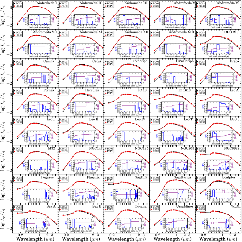
Figure 1.— Broadband FUV-to-$M$ SEDs (i.e. FUV, NUV, $U$, $u$, $B$, $g$, $V$, $r$, $R$, $i$, $I$, $z$, $y$, $J$, $H$, $K$, $L$, and $M$) of the 40 LG dwarf galaxies predicted by the resolved CMD-based SFHs and metallicity evolution histories. The monochromatic luminosities in all passbands have been normalized by the $i$ band luminosities. The SEDs generated based on the BC03 models and the FSPS models are shown as black and red dots respectively. The inset plot in each panel shows the normalized SFHs and metallicity evolution histories as determined by Cole et al. (2007, 2014) for Leo A and DDO 210, by Hidalgo et al. (2011) for LGS 3, and by Weisz et al. (2014) for the remaining galaxies.

II.3. Expanding the LG sample by Assigning New Metallicities and Varying the SFHs in the Recent 1 Gyr

The original sample of 40 LG dwarfs introduced above covers a variety of SFHs, as (for instance) quantified by the spread of mass-weighted stellar population ages (see Fig. 2), and thus offers us a unique opportunity to investigate the dependence of stellar mass estimates on real SFHs. In order to explore the impact of metallicities on stellar mass estimates, starting from the SFH of each LG dwarf galaxy, we draw new mass-weighted metallicities from a uniform grid of metallicities with an interval of 0.3 dex and a range of $-1.95$ to 0.22 in [M/H] and then create new composite stellar populations with the same shape of SFH and metallicity evolution history but with the newly drawn mass-weighted metallicities. Since metallicities generally increase with time along given metallicity evolution histories, [M/H] of the recently formed (or ancient) stellar populations resulting from our expansion of the weighted-[M/H] coverage would be $>$ 0.22 (or $<$ $-1.95$) in some cases. We exclude these cases from our final expanded sample. The exercise of expanding the sample with [M/H] is justified by a lack of significant correlation between SFHs and [M/H] of the LG dwarfs (Fig. 2). By doing so, we expand the original sample size from 40 to 251.

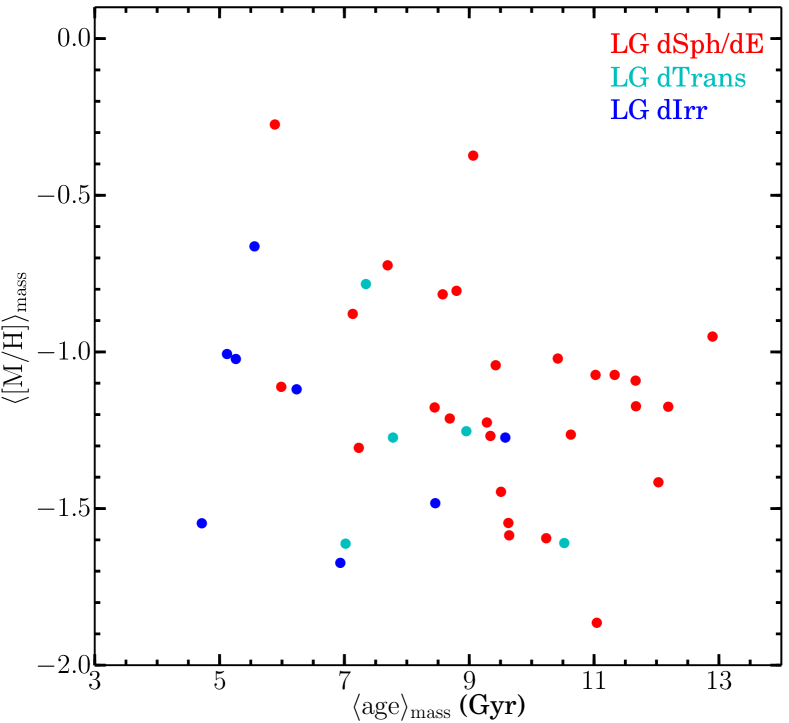
Figure 2.— Mass-weighted ages $\langle{\rm age}\rangle_{\rm mass}$ and mass-weighted metallicities $\langle[\rm M/H]\rangle_{\rm mass}$ of the 40 LG dwarf galaxies studied in this work.

Our sample of LG dwarf galaxies lacks extreme starbursts. The “burst phase” of local galaxies can be usually attributed to environmental influences, such as galaxy interactions and cosmic gas accretion. Starburst events are short-lived and thus are not necessarily relevant to the past SFHs of their host galaxies. In order to explore the influence of recent burst or suppression of star formation on stellar mass estimates, we add new composite stellar populations by varying the relative strengths of star formation in the recent 1 Gyr of the original SFHs. Specifically, for each “galaxy” in the above [M/H]-expanded sample, the recent 1 Gyr is divided into three age bins that are separated at lookback times of 0.1 and 0.4 Gyr, then the average SFRs in each age bin are independently drawn from a grid of seven values: 0.0, 0.1, 0.3, 1.0, 2.0, 5.0, and 10.0 times the lifetime-averaged SFR of the SFH in question. A maximum average burst strength (a.k.a. birth-rate parameter, as defined by Scalo 1986) of 10 over $\sim$100 Myr matches that of the extreme starbursts observed in nearby galaxies (e.g. McQuinn et al. 2010). The birth-rate parameters smaller than 1 mimic truncated SFHs expected for galaxies that are abruptly stripped off their gas supply in dense environments such as galaxy clusters. By doing so, our full sample size is increased by another 86,064, and thus the final sample to be analyzed for the major part of this paper includes 86,344 “galaxies” with different SFHs. Note that this exercise of expanding the parameter coverage of recent SFHs does not apply to cases where the relative star formation strengths of the original SFHs averaged over the relevant lookback times are already in accord with the corresponding values to be drawn from the grid in the expanded parameter space. The corresponding broadband SEDs and SFH-related parameters of the expanded sample are derived as with the original sample (Section II.2.4). In the rest of this paper, we will refer to this expanded sample of 86,344 unique combinations of SFHs and metallicity evolution histories, with the SMC-bar extinction curve and a $A_{V,{\rm young}}$ of 0.5 mag, as our default full sample.

III. Methodology of SED fitting

III.1. A Brief Review

Solving for the constituent stellar populations of different mass-to-light ratios ($\Upsilon_{\star}$) based on observed SEDs is an ill-posed problem, as mentioned in the Introduction. There are two distinctly different techniques for fitting SEDs of galaxies. One is the “Bayesian template fitting” approach, which generally involves Bayesian inferences of physical parameters through comparisons of the observed SEDs and model SEDs from a predefined library of template SFHs. The library of template SFHs, being either precomputed or computed on the fly, are usually built with simplified parameterization and/or strong prior assumptions of the lifetime SFHs. The other one is the “inversion” approach, where the observed SEDs are inverted into as many independent SSP components as necessary, with the weights assigned to individual components being solved on the fly. A recent review on different fitting techniques was given by Walcher et al. (2011).

The Bayesian template fitting method is so far the most commonly used one for fitting broadband SEDs (e.g. Silva et al. 1998; Bolzonella et al. 2000; Brammer et al. 2008; da Cunha, Charlot & Elbaz 2008; Noll et al. 2009; Acquaviva et al. 2011; Arnouts & Ilbert 2011; Pacifici et al. 2012; Johnson et al. 2013b; Han & Han 2014; Chevallard & Charlot 2016; Iyer & Gawiser 2017, among many others), but it can be severely limited/biased by the prior assumptions on the form (e.g. exponentially declining) of template SFHs. To avoid a simplified assumption on the parametric form of model SFHs, Zhang et al. (2012) adopted a non-parametric method by building a library of model SFHs which are characterized by six independent logarithmically-spaced star formation periods. Leja et al. (2017) also presented a non-parametric method through a Monte Carlo Marko Chain (MCMC) sampling of the posterior distributions of SFHs characterized by six independent star formation periods. The inversion approach, which is realized through either Monte Carlo simulations or direct (non)linear matrix inversion, is nonparametric and is in principle the unbiased way to fit for stellar populations of galaxies, as long as the full parameter space can be explored. The inversion approach has been mostly applied to fitting of spectroscopic data (e.g. Ocvirk et al. 2006b; Tojeiro et al. 2007; Cappellari 2017), with the exception of Blanton & Roweis (2007).

III.2. Nonparametric SED fitting: The Matrix Inversion with NNLS Optimization

One important goal of this work is to explore the efficacy of broadband SED fitting for recovering the integrated stellar mass of galaxies, without any prior assumption on the SFHs. Here we introduce a pure mathematical matrix inversion method for broadband SED fitting.

Any SFHs can be decomposed into a series of SSPs with different ages, metallicities, and masses (or weights). As long as the nonlinear dependence on extinction can be treated separately, decomposing the observed SEDs into that of a series of SSPs is mathematically an underdetermined non-negative linear matrix inversion process (e.g. Press et al. 1992). To implement this approach, we turn to the classical Active-set algorithm, first introduced by Lawson & Hanson (1974). The Active-set algorithm solves the non-negative matrix inversion problem by iteratively minimizing the quadratic residual. In our particular case, starting from an “active set” that contains all SSP components that constitute the design matrix, at each iteration, the SSP component in the “active set” that maximizes the negative gradient of the quadratic residual and at the same time leads to a non-negative solution to the normal equation is removed from the “active set” and added to a “passive set” or solution space that contains the SSP components that result in the final non-negative solution vector of weights that minimizes the quadratic residual. Recent studies suggest that the non-negative regularized least-squares regression can be remarkably effective even in cases where the data sample size is smaller than the dimensions of the parameter space (e.g. Meinshausen 2013), as long as the solution vector is known to be sparse, i.e. only a subset of the solution vector is not equal to zero.

To apply the above NNLS method to our broadband SED fitting, we adopt a base of 180 SSPs, encompassing 15 ages uniformly distributed in log space between 0.001 and 14 Gyr, and a grid of 12 metallicity $Z$ values ranging from 2$\times$10^-4 to 0.03 (or [M/H] from $-$1.95 to 0.22, for $Z_{\odot}$ = 0.018). Note that the 12 metallicity values are selected to be every other value as provided by the Padova+BaSeL isochrones used in the FSPS models. We then use the Lawson & Hanson NNLS algorithm through a Python wrapper of the original FORTRAN code (scipy.optimize.nnls) to solve for non-negative weights of SSPs, given any “observed” input SED. The same NNLS code has been used in the pPXF software (Cappellari 2017) for full-spectrum fitting.

We consider NNLS SED fitting to our default full sample, with $A_{V,{\rm young}}$ being either fixed to 0.5 mag or a free parameter in the fitting, following the same extinction recipes as described in Section II.2.3. To fit SEDs with $A_{V,{\rm young}}$ as a free parameter, we run two successive iterations of NNLS SED fitting with decreasing step sizes of $A_{V,{\rm young}}$ in order to find the global minimum. In particular, the first iteration of fitting goes through a grid of $A_{V,{\rm young}}$ values ranging from 0.0 to 2.0 mag with a step size of 0.1 mag, and then a second iteration goes through a finer grid of $A_{V,{\rm young}}$ with a step size of 0.03 mag and centered around the $A_{V,{\rm young}}$ value that leads to the minimum $\chi^{2}$ in the first iteration.

A vast majority of previous works on SED modeling assumed constant metallicities along individual model SFHs, without taking into account metallicity evolution. Gallazzi & Bell (2009) found that stellar masses may be systematically over- or underestimated (depending on the average ages) when using monometallic (exponential) model SFHs to fit SEDs resulting from variable-metallicity SFHs. Here we consider both monometallic and multimetallic SFH solutions in our NNLS fitting. In particular, for multimetallic SFH solutions, all of the 180 SSP templates are used at the same time to search for the non-negative solutions, while for monometallic SFH solutions, 12 candidate monometallic solutions for the 12 metallicity values are first found by putting separately each set of SSP templates of the same metallicity in the “active set” to search for non-negative solutions, and then the final best-fit solution vector is selected as the one leading to the minimum $\chi^{2}$.

Every SSP component is normalized to a total stellar mass of 1 $M_{\odot}$, so the total mass corresponding to a given NNLS solution vector is simply a sum of the weights of individual SSP components. For each input SED, the NNLS fitting is performed for 500 times with random Gaussian noise added at each time. Then the 50th percentile of the resulting distribution of the 500 best-fit stellar masses is adopted as the most probable stellar mass, and the 16th and 84th percentiles as the 1-$\sigma$ confidence intervals. The results of our SED fitting to the default full sample will be presented in Section VI.

IV. Color–Mass-to-Light Ratio Relations

IV.1. The Context

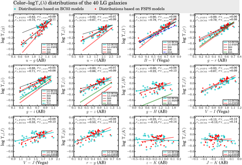
Figure 3.— Distributions of the 40 LG dwarf galaxies studied in this work on various color–mass-to-light-ratio (color–$\log\Upsilon_{\star}$) diagrams. The red filled circles and cyan open circles represent the distributions of the 40 galaxies based on SFHs reconstructed with the FSPS and BC03 models, respectively. The black solid lines and cyan short-dashed lines represent the linear regression of the color–$\log\Upsilon_{\star}$distributions based on the FSPS and BC03 models, respectively. Several published linear color–$\log\Upsilon_{\star}$($\lambda$) relations (whenever available for given passbands) are also plotted for comparison. In particular, these published relations are respectively from Bell et al. (2003; B03), Zibetti et al. (2009; Z09), Taylor et al. (2011; T11), Roediger & Courteau (2015; R15), and Herrmann et al. (2016; H16). The line styles and colors of these overplotted relations are as indicated in the legends of individual panels. Except for the B03 relations, which were calibrated based on the PEGASE models, all the other relations were based on either the original (i.e. T11, R15) or the updated (i.e. Z09, H16) BC03 models. The PEGASE models were based on about the same isochrones as BC03. Therefore, the differences between different relations in the optical bands primarily reflect the different priors of SFHs assumed in the different studies.

The color–$\Upsilon_{\star}$($\lambda$) relations provide a cheap way to estimate stellar masses of galaxies (Bell & de Jong 2001). Linear color–$\log\Upsilon_{\star}$($\lambda$) relations of galaxies have been calibrated in different passbands by numerous studies in the past. To name a few, these studies include Bell & de Jong (2001), Bell et al. (2003, hereafter B03), Portinari et al. (2004), Zibetti et al. (2009, hereafter Z09), Taylor et al. (2011, hereafter T11), Into & Portinari (2013), Roediger & Courteau (2015, hereafter R15), Herrmann et al. (2016, hereafter H16), etc. These studies calibrated linear color–$\log\Upsilon_{\star}$($\lambda$) relations with sometimes significantly different slopes and zero points (or intercepts). What is even more worrisome, McGaugh & Schombert (2014) found that all of the commonly employed relations fail to provide self-consistent results, in the sense that the same set of relations (i.e. the ones from the same authors) gives systematically different stellar mass estimates when different passbands are used for given galaxies.

The effectiveness of single colors as indicators of $\Upsilon_{\star}$($\lambda$) may rely on the partially compensating effect of ages, metallicities and dust reddening on colors, and therefore $\Upsilon_{\star}$($\lambda$), in the sense that an increase of any of these three parameters generally results in a reddening of colors and an increase of $\Upsilon_{\star}$($\lambda$). This interpretation is straightforward to understand for SSPs, but not for composite stellar populations whereby the integrated light in different passbands may be dominated by different stellar populations and the light-dominant populations may not be the mass-dominant ones. The location of a galaxy on the color–$\Upsilon_{\star}$ diagrams is in principle determined by its SFH, metallicity evolution history, and dust reddening.

The impact of SFHs on colors and $\Upsilon_{\star}$($\lambda$) may be reflected by the mass-weighted ages $\langle{\rm age}\rangle_{\rm mass}$ and the monochromatic light-weighted ages $\langle{\rm age}\rangle_{\rm\lambda}$ in passbands of different wavelengths $\lambda$. The impact of metallicity evolution on colors and $\Upsilon_{\star}$($\lambda$) may be reflected by the mass-weighted metallicities $\langle[\rm M/H]\rangle_{\rm mass}$ and the monochromatic light-weighted metallicities $\langle{\rm[M/H]}\rangle_{\rm\lambda}$ in different passbands. In what follows in this section, we will use the mass- and light-weighted quantities mentioned above, together with the lookback times when 20% (t_m,20%) and 80% (t_m,80%) of total stellar masses were formed, to investigate how SFHs and metallicity evolution affect the color–$\Upsilon_{\star}$($\lambda$) distributions. Note that we will use $\langle{\rm age}\rangle_{\lambda,{\rm long}}$ and $\langle{\rm age}\rangle_{\lambda,{\rm short}}$ to represent $\langle{\rm age}\rangle_{\rm\lambda}$ at the longer- and shorter-wavelength passbands involved in a given color, and $\langle{\rm[M/H]}\rangle_{\lambda,{\rm long}}$ and $\langle{\rm[M/H]}\rangle_{\lambda,{\rm short}}$ to represent monochromatic light-weighted [M/H] at the longer- and shorter-wavelength passbands involved in a given color.

IV.2. Distribution of LG Dwarf Galaxies

A selection of representative color–$\log\Upsilon_{\star}$($\lambda$) relations of the LG dwarf galaxies is shown in Figure 3. A majority of previous studies of galaxy stellar masses were carried out with the BC03 models. Therefore, we generate the color–$\log\Upsilon_{\star}$($\lambda$) relations of the LG dwarfs based on both our default FSPS models (red filled circles) and the BC03 models (cyan open circles), in order to facilitate a fair comparison with other studies. Following the common practice, we conducted linear least-squares regression to the color–$\log\Upsilon_{\star}$($\lambda$) distributions. The fitted linear relations are overplotted on the distributions shown in Figure 3. We also calculate the Spearman’s rank correlation coefficients $r_{s,{\rm FSPS}}$ and $r_{s,{\rm BC03}}$ between colors and $\log\Upsilon_{\star}$($\lambda$), and the standard deviations $\sigma_{\Upsilon_{\star},{\rm FSPS}}$ and $\sigma_{\Upsilon_{\star},{\rm BC03}}$ of $\log\Upsilon_{\star}$($\lambda$) around the best-fit linear relations. Both the Spearman’s rank correlation coefficients and the standard deviations are listed at the top of each panel of Figure 3.

From Figure 3, we can see that SFHs constructed with the FSPS and BC03 models give color–$\log\Upsilon_{\star}$($\lambda$) relations (e.g. the slopes and intercepts of the linear fits) that are in decent agreement across the whole wavelength range. Nevertheless, we notice that the FSPS models give significantly tighter color–$\log\Upsilon_{\star}$($\lambda$) relations than the BC03 models, which is quantified by both the systematically higher correlation coefficients and the overall smaller scatters for the FSPS models. These differences might be primarily attributed to the different versions of Padova isochrones used by the two models.

Several linear color–$\log\Upsilon_{\star}$($\lambda$) relations calibrated by previous studies are also overplotted in Figure 3 for a visual comparison. The references to these literature relations are given in the caption of Figure 3. These plotted linear relations are the ones in the literature that were calibrated based on either the original or updated BC03 models. Here we just point out that the LG dwarfs follow color–$\log\Upsilon_{\star}$($\lambda$) relations that fall in between the extreme ones calibrated by previous studies. A more detailed discussion about these relations and their differences will be given in Section VII.1. In the Appendix section, we present the linear least-squares fitting to various optical color–$\log\Upsilon_{\star}$($\lambda$) relations of the 40 LG dwarf galaxies and the expanded samples in Tables 1 and 2.

IV.3. Impact of SFHs on color–$\log\Upsilon_{\star}$($\lambda$) Relations

We use the (expanded) default full sample to explore the impact of SFHs on color–$\log\Upsilon_{\star}$($\lambda$) distributions. In what follows in this subsection, we show the color–$\log\Upsilon_{\star}$($\lambda$) distributions of the default full sample, which are grouped by different ranges of aforementioned parameters, including $\langle{\rm age}\rangle_{\rm mass}$ (Fig. 4), $\log$(t_m,20%/t_m,80%) (Fig. 5), $\langle{\rm age}\rangle_{\lambda,{\rm long}}$ (Fig. 6), and ($\log\langle{\rm age}\rangle_{\lambda,{\rm short}}$$-$$\log\langle{\rm age}\rangle_{\rm mass}$) (Fig. 7). In addition, Figure 8 presents the color–$\log\Upsilon_{\star}$($V$) distributions, which are grouped by $\langle{\rm age}\rangle_{V}$ in order to demonstrate the variation of given $\log\Upsilon_{\star}$($\lambda$) as functions of different colors. To generate the distributions shown in Figures 4 to 7, the color–$\log\Upsilon_{\star}$($\lambda$) two-dimensional histograms of number densities $N$ of data points with bin sizes of 0.02$\times$0.02 are first created, and then contours enclosing the relevant area with $N>0$ are plotted.

IV.3.1 Correlations with $\langle{\rm age}\rangle_{\rm mass}$

As a zero-order representation of SFHs, $\langle{\rm age}\rangle_{\rm mass}$ is barely correlated with either colors or $\log\Upsilon_{\star}$($\lambda$) (see Fig. 4). However, $\langle{\rm age}\rangle_{\rm mass}$ appears to be positively correlated with the lower and especially upper bounds of $\log\Upsilon_{\star}$($\lambda$) for given color values, and this $\langle{\rm age}\rangle_{\rm mass}$-dependent effect is more significant for redder color values, leading to more positive average slopes of the color–$\log\Upsilon_{\star}$($\lambda$) relations for galaxies with larger $\langle{\rm age}\rangle_{\rm mass}$. Moreover, the slope differences for different $\langle{\rm age}\rangle_{\rm mass}$ are larger for optical colors covering longer-wavelength baselines. For instance, the slope differences between subsamples with $\langle{\rm age}\rangle_{\rm mass}$ = 11–13 Gyr and $\langle{\rm age}\rangle_{\rm mass}$ = 3–5 Gyr (Fig. 4) are $\sim$ 0.01 and $\sim$ 0.11, respectively, for the ($B$$-$$V$)–$\log\Upsilon_{\star}$($V$) and ($g$$-$$z$)–$\log\Upsilon_{\star}$($z$) relations. We also note that subsamples with younger $\langle{\rm age}\rangle_{\rm mass}$ have tighter and more linear color–$\log\Upsilon_{\star}$($\lambda$) relations than those with older $\langle{\rm age}\rangle_{\rm mass}$. This implies that $\Upsilon_{\star}$($\lambda$) of higher-redshift galaxies is generally better constrained as long as the redshift information is used to restrict the oldest possible $\langle{\rm age}\rangle_{\rm mass}$.

IV.3.2 Correlations with SFH “concentration”

In analogy to the definition of concentration of galaxy light profiles (e.g. Bershady et al. 2000), log(t_m,20%/t_m,80%) can be used to quantify the “concentration” of SFHs in time (Figure 5). Subsamples with larger $\log$(t_m,20%/t_m,80%) (i.e. more extended SFHs) cover smaller ranges of colors and $\Upsilon_{\star}$($\lambda$). However, subsamples with different $\log$(t_m,20%/t_m,80%) follow color–$\log\Upsilon_{\star}$($\lambda$) correlations with very similar slopes, and except for those with the smallest $\log$(t_m,20%/t_m,80%) (i.e. $\sim$ 0.0 – 0.3, the most concentrated SFHs), similar intercepts.

IV.3.3 Correlations with $\langle{\rm age}\rangle_{\rm\lambda}$

The monochromatic light-weighted ages, e.g. $\langle{\rm age}\rangle_{\lambda,{\rm long}}$ (Figures 6 and 8), are broadly correlated with $\log\Upsilon_{\star}$($\lambda$). Similar to the findings of Worthey (1994) for SSPs, we point out that the correlation coefficients between $\langle{\rm age}\rangle_{\rm\lambda}$ and $\log\Upsilon_{\star}$($\lambda$) peak in $J$ band ($r_{s}\!=\!0.96$), with the correlation being poorer toward both longer- and shorter-wavelength luminance passbands. In addition, for a given combination of color and $\log\Upsilon_{\star}$($\lambda$), the relations defined by subsamples of different $\langle{\rm age}\rangle_{\lambda,{\rm long}}$ run largely parallel to each other, and the perpendicular (i.e. normal to the running directions of color–$\log\Upsilon_{\star}$($\lambda$) correlations) offset between them becomes smaller for shorter-wavelength luminance passband and optical colors that involve the $g$ or $B$ band as the shorter-wavelength passband and at the same time cover shorter-wavelength baselines (e.g. $B$$-$$V$, $g$$-$$r$). In particular, we note that the ($B$$-$$V$)–$\log\Upsilon_{\star}(V)$ relation is the one with the least “perpendicular offset” between subsamples of different $\langle{\rm age}\rangle_{\lambda,{\rm long}}$, whereas the color–$\log\Upsilon_{\star}$($\lambda$) relations involving NIR passbands are the ones with the largest “perpendicular offsets.” A smaller “perpendicular offset” suggests a smaller systematic dependence on $\langle{\rm age}\rangle_{\rm\lambda}$.

IV.3.4 Mismatches between $\langle{\rm age}\rangle_{\rm\lambda}$ and $\langle{\rm age}\rangle_{\rm mass}$

Mismatches between light- and mass-weighted ages, e.g. $\log\langle{\rm age}\rangle_{\lambda,{\rm short}}$$-$$\log\langle{\rm age}\rangle_{\rm mass}$ (Figure 7) reflect the degree of the “outshining” effect of younger light-dominant populations over older mass-dominant populations. Subsamples with $\log\langle{\rm age}\rangle_{\lambda,{\rm short}}$$-$$\log\langle{\rm age}\rangle_{\rm mass}$ $\lesssim$ $-0.6$ tend to have slightly steeper color–$\log\Upsilon_{\star}$($\lambda$) correlations, and this steepening trend is sharper for colors covering longer-wavelength baselines. The effect of mismatches between $\log\langle{\rm age}\rangle_{\lambda,{\rm short}}$ and $\log\langle{\rm age}\rangle_{\lambda,{\rm long}}$ (not shown in this paper) is very similar to that between $\log\langle{\rm age}\rangle_{\lambda,{\rm short}}$ and $\log\langle{\rm age}\rangle_{\rm mass}$.

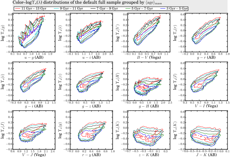
Figure 4.— Impact of mass-weighted ages, $\langle{\rm age}\rangle_{\rm mass}$, on color–$\log\Upsilon_{\star}$($\lambda$) distributions of the default full sample. The solid contours of different colors in each panel enclose the distributions of five subsamples with different ranges of $\langle{\rm age}\rangle_{\rm mass}$, as indicated in the figure title.

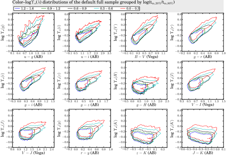
Figure 5.— Impact of “concentration” of SFHs (in time) on color–$\log\Upsilon_{\star}$($\lambda$) distributions of the default full sample. Here the sample is grouped into subsamples of different $\log$(t_m,20%/t_m,80%), where t_m,20% and t_m,80% are the lookback times when 20% and 80% of the total stellar masses were formed, respectively. The solid contours of different colors in each panel enclose the distributions of five subsamples with different ranges of $\log$(t_m,20%/t_m,80%), as indicated in the figure title.

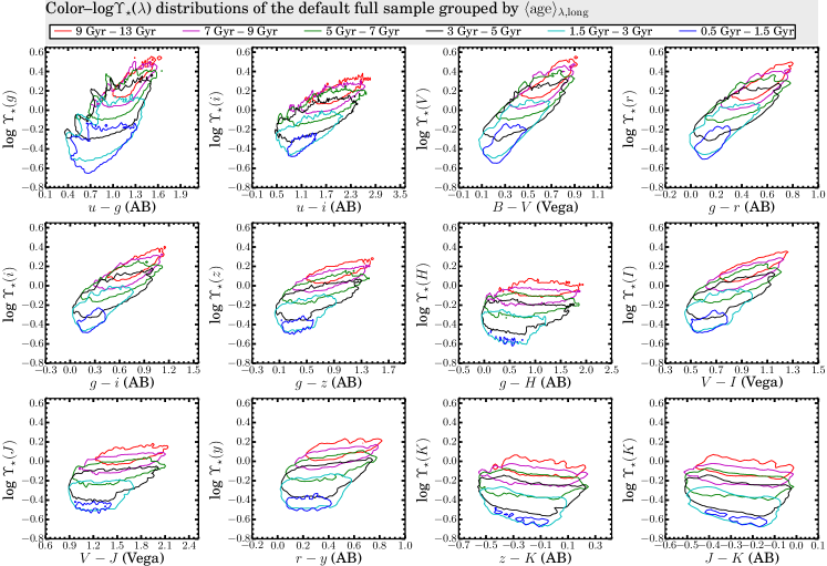
Figure 6.— Impact of monochromatic light-weighted ages on color–$\log\Upsilon_{\star}$($\lambda$) distributions of the default full sample. Here the sample is grouped into subsamples of different $\langle{\rm age}\rangle_{\lambda,{\rm long}}$which represents the monochromatic light-weighted ages of the longer-wavelength passband involved in each color. The solid contours of different colors in each panel enclose the distributions of five subsamples with different $\langle{\rm age}\rangle_{\lambda,{\rm long}}$, as indicated in the figure title.

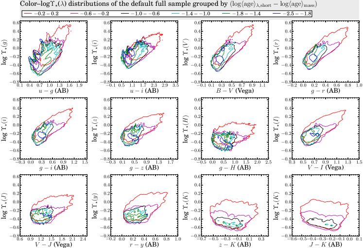
Figure 7.— Impact of the “outshining” effect of the light-dominant young populations over mass-dominant old populations on color–$\log\Upsilon_{\star}$($\lambda$) distributions of the default sample. Here the full sample is grouped into subsamples of different ranges of log$\langle{\rm age}\rangle_{\lambda,{\rm short}}$$-$log$\langle{\rm age}\rangle_{\rm mass}$, where $\langle{\rm age}\rangle_{\rm mass}$ represents the mass-weighted age and $\langle{\rm age}\rangle_{\lambda,{\rm short}}$ represents the monochromatic light-weighted ages of the shorter-wavelength passband involved in a given color. The solid contours in each panel enclose the distributions of subsamples with different log$\langle{\rm age}\rangle_{\lambda,{\rm short}}$$-$log$\langle{\rm age}\rangle_{\rm mass}$, as indicated in the figure title.

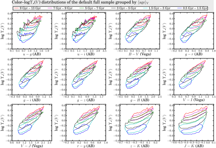
Figure 8.— Same as Figure 6, but here for color–$\log\Upsilon_{\star}$($V$) distributions.

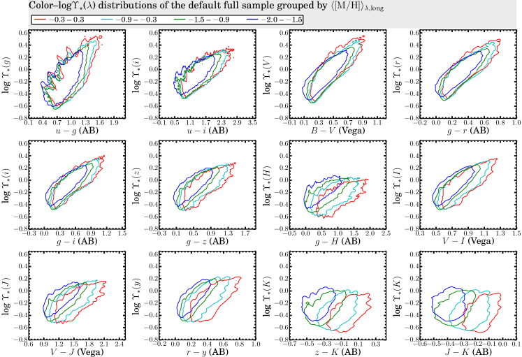
Figure 9.— Impact of light-weighted metallicities on color–$\log\Upsilon_{\star}$($\lambda$) relations of the full sample. Here the sample is grouped into subsamples of different ranges of $\langle{\rm[M/H]}\rangle_{\lambda,{\rm long}}$. $\langle{\rm[M/H]}\rangle_{\lambda,{\rm long}}$ represents the monochromatic light-weighted [M/H] of the longer-wavelength passband involved in each color. The solid contours in each panel enclose the distributions of four subsamples with different ranges of $\langle{\rm[M/H]}\rangle_{\lambda,{\rm long}}$, as indicated in the figure title.

IV.4. Impact of metallicity evolution on color–$\log\Upsilon_{\star}$($\lambda$) Relations

IV.4.1 Impact of Average Metallicities

As in Figures 4 – 7, color–$\log\Upsilon_{\star}$($\lambda$) distributions of the default full sample grouped by light-weighted metallicities $\langle{\rm[M/H]}\rangle_{\lambda,{\rm long}}$ are shown in Figure 9. The distributions with respect to $\langle[\rm M/H]\rangle_{\rm mass}$ are very similar to those with respect to $\langle{\rm[M/H]}\rangle_{\lambda,{\rm long}}$, so they are not shown here.

Subsamples with higher $\langle{\rm[M/H]}\rangle_{\lambda,{\rm long}}$ follow color–$\log\Upsilon_{\star}$($\lambda$) relations that are slightly steeper and have a higher degree of nonlinearity than those with lower $\langle{\rm[M/H]}\rangle_{\lambda,{\rm long}}$, owing to the fact that more metal-rich stellar atmospheres leave a stronger and nonlinear imprint on specific SED regions. Moreover, subsamples with higher $\langle{\rm[M/H]}\rangle_{\lambda,{\rm long}}$ generally have a larger spread of $\Upsilon_{\star}$($\lambda$) at given color values. The “perpendicular offsets” between the color–$\log\Upsilon_{\star}$($\lambda$) relations of subsamples with different $\langle{\rm[M/H]}\rangle_{\lambda,{\rm long}}$ are larger for colors involving longer-wavelength passbands, in line with the well-known higher sensitivity of colors covering longer wavelength baselines to stellar atmosphere metallicities.

$\Upsilon_{\star}$($\lambda$) has relatively tight correlations with optical–optical colors but not optical–NIR or (especially) NIR-NIR colors. This is because both $\Upsilon_{\star}$($\lambda$) and optical–optical colors have a stronger correlation with $\langle{\rm age}\rangle_{\rm\lambda}$ than $\langle{\rm[M/H]}\rangle_{\rm\lambda}$, whereas optical–NIR colors depend about equally on both $\langle{\rm age}\rangle_{\rm\lambda}$ and $\langle{\rm[M/H]}\rangle_{\rm\lambda}$, and NIR–NIR colors primarily on $\langle{\rm[M/H]}\rangle_{\rm\lambda}$.

IV.4.2 Impact of the Metallicity Evolution

Nearly all previous studies on stellar mass estimates do not take into account metallicity evolution when building their model SFH libraries. Here we explore the differences between color–$\log\Upsilon_{\star}$($\lambda$) distributions resulting from the multimetallic SFHs (the default in this work) and the unrealistic monometallic SFHs. To this end, for every “galaxy” in the default full sample, we determine two additional sets of multiband SEDs resulting from the same SFH but with a single [M/H] fixed to either $\langle[\rm M/H]\rangle_{\rm mass}$ or the $V$-band light-weighted $\langle{\rm[M/H]}\rangle_{V}$. The color–$\log\Upsilon_{\star}$($\lambda$) distributions for the samples with multimetallic and monometallic SFHs are shown separately in Figure 10. In addition, we also derive the differences of colors ($\Delta$[color]) and $\log\Upsilon_{\star}$($\lambda$) ($\Delta$[$\log\Upsilon_{\star}$($\lambda$)]) between the monometallic and multimetallic “versions” of each galaxy, and the corresponding contours enclosing the $\Delta$(color) vs. $\Delta$($\log\Upsilon_{\star}$($\lambda$)) distributions of the samples are shown as inset plots of Figure 10. We note that the conclusions drawn below do not change if monometallic SFHs with [M/H] fixed to light-weighted [M/H] in passbands other than $V$ are used.

The multimetallic and monometallic SFHs result in about the same coverage on the color–$\log\Upsilon_{\star}$($\lambda$) planes. The color–$\log\Upsilon_{\star}$($\lambda$) relations of monometallic SFHs are generally slightly shallower (especially for the ones with [M/H] = $\langle[\rm M/H]\rangle_{\rm mass}$) but still in good agreement with that of multimetallic SFHs (see the solid linear least-squares regression lines in each panel of Figure 10). Nevertheless, the multimetallic SFHs match the monometallic SFHs with [M/H] = $\langle{\rm[M/H]}\rangle_{V}$ better than those with [M/H] = $\langle[\rm M/H]\rangle_{\rm mass}$. In particular, the relative slope differences of monometallic SFHs of [M/H] = $\langle{\rm[M/H]}\rangle_{V}$ with respect to the multimetallic SFHs are ($\lesssim$ 0.3% – 3%) generally one order of magnitude smaller than those of monometallic SFHs of [M/H] = $\langle[\rm M/H]\rangle_{\rm mass}$ ($\sim$ 5% – 30%). Note that the relative slope differences for the NIR color–$\log\Upsilon_{\star}$($\lambda$) relations are larger than for the optical color–$\log\Upsilon_{\star}$($\lambda$) relations. Moreover, the half max–min ranges of $\Delta$$\log\Upsilon_{\star}$($\lambda$) and $\Delta$(colors) resulting from the monometallic and multimetallic versions of any given SFHs are also generally smaller when [M/H] is fixed to $\langle{\rm[M/H]}\rangle_{V}$.

As shown in the inset plots of Figure 10, $\Delta$$\log\Upsilon_{\star}$($\lambda$) distributions extend to about 2$\times$ larger ranges (by $\gtrsim$ 0.05 dex and 0.10 dex for [M/H] = $\langle{\rm[M/H]}\rangle_{V}$ and [M/H] = $\langle[\rm M/H]\rangle_{\rm mass}$, respectively) above than below $\Delta$$\log\Upsilon_{\star}$($\lambda$) = 0, suggesting that the monometallic versions of given SFHs tend to predict higher $\log\Upsilon_{\star}$($\lambda$) than the multimetallic versions. Because the differences between stellar masses resulting from the monometallic and multimetallic SFHs are negligible ($<$ 0.01 dex), the tendency of monometallic SFHs having higher $\log\Upsilon_{\star}$($\lambda$) can be explained if the relatively old stars have higher [M/H] and thus lower luminosities in the monometallic SFHs than in the multimetallic SFHs. In addition, we note that the half max–min ranges of $\Delta$$\log\Upsilon_{\star}$($\lambda$) for the monometallic SFHs with [M/H] = $\langle{\rm[M/H]}\rangle_{V}$ are generally $\lesssim$ 0.1 dex, and the half max–min ranges of $\Delta$(color) are $\lesssim$ 0.1 for optical–optical/NIR–NIR colors, $\lesssim$ 0.2 for UV–optical colors, and $\lesssim$ 0.3 for optical–NIR colors.

Lastly, we note that subsamples with larger $\langle{\rm age}\rangle_{\rm mass}$ have relatively larger slope differences between color–$\log\Upsilon_{\star}$($\lambda$) relations of monometallic and multimetallic SFHs, and they also have larger half max–min ranges of $\Delta$$\log\Upsilon_{\star}$($\lambda$) and $\Delta$(colors) than subsamples with smaller $\langle{\rm age}\rangle_{\rm mass}$. We mention that the nearly 2$\times$ larger ranges of $\Delta$$\log\Upsilon_{\star}$($\lambda$) above than below 0 mentioned above exist independently of $\langle{\rm age}\rangle_{\rm mass}$. The relative slope differences for optical color–$\log\Upsilon_{\star}$($\lambda$) relations vary from $\sim$ 5% for $\langle{\rm age}\rangle_{\rm mass}$ =11 – 14 Gyr to $\lesssim$ 1% for $\langle{\rm age}\rangle_{\rm mass}$ =3 – 5 Gyr.

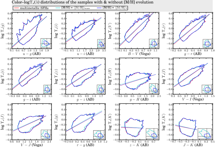
Figure 10.— Comparison of color–$\log\Upsilon_{\star}$($\lambda$) distributions resulting from SFHs with and without accompanied metallicity evolution, i.e. multimetallic and monometallic SFHs. The red contours mark coverage of our default color–$\log\Upsilon_{\star}$($\lambda$) distributions with multimetallic SFHs, whereas the cyan and blue contours mark the color–$\log\Upsilon_{\star}$($\lambda$) coverage of distributions resulting from monometallic SFHs with the [M/H] being fixed to $\langle[\rm M/H]\rangle_{\rm mass}$ and $\langle{\rm[M/H]}\rangle_{V}$, respectively. The linear least-squares regression to the three distributions is represented by the solid lines, with the same color scheme as for the contours. The inset plot at the lower right corner of each panel shows contours (cyan for [M/H]=$\langle[\rm M/H]\rangle_{\rm mass}$; blue for [M/H]=$\langle{\rm[M/H]}\rangle_{V}$) enclosing the distributions of $\Delta$(color) (horizontal axis) vs. $\Delta$log($\Upsilon_{\star}$($\lambda$)) (vertical axis), where $\Delta$(color) and $\Delta$log($\Upsilon_{\star}$($\lambda$)) are, respectively, the color differences and $\log$($\Upsilon_{\star}$($\lambda$)) differences between the same SFHs without and with metallicity evolution. The position of $\Delta$(color) = 0 and $\Delta$log($\Upsilon_{\star}$($\lambda$)) = 0 coincides with the horizontal and vertical lines (cross-hair) in the inset plot of each panel. The inset and main plots in each panel share the same axis scale.

IV.5. Impact of Dust Extinction and Dust Extinction Curves on color–$\log\Upsilon_{\star}$($\lambda$) Relations

Dust extinction and reddening have been generally regarded as at most a secondary effect on stellar mass estimation, due to the partially counteracting effect of dust reddening and stellar aging on the color–$\log\Upsilon_{\star}$($\lambda$) planes (e.g. Bell & de Jong 2001). However, as we will show below, the influence of dust extinction and reddening on color–$\log\Upsilon_{\star}$($\lambda$) distributions of real galaxies depends on several factors, including the dust extinction curves, the amount of dust extinction, the wavelength ranges, and SFHs.

Here we explore how the color–$\log\Upsilon_{\star}$($\lambda$) distributions of our samples vary with dust extinction and dust extinction curves. To this end, for every “galaxy” in our default full sample, we derive additional sets of multiband SEDs by applying $A_{V,{\rm young}}$ values other than our default 0.5 mag and using the relatively shallow Charlot & Fall (2000; CF00) dust extinction curve where $A_{\lambda}$ $\propto$ $\lambda^{-0.7}$. For reference, the SMC-bar dust extinction curve can be fitted with a power-law index of $\simeq$ $-$1.2 in the optical wavelength range. The resultant color–$\log\Upsilon_{\star}$($\lambda$) distributions of the $A_{V,{\rm young}}$-expanded and the default full samples are shown in Figure 11.

IV.5.1 Impact of the Amount of Dust Extinction

In the age-dependent dust extinction recipe adopted in this work, the free parameter is the $V$-band extinction suffered by populations younger than 40 Myr ($A_{V,{\rm young}}$). Extinction linearly decreases with stellar ages from the maximum at ages $\leq$ 40 Myr to zero at ages $\geq$ 100 Myr. Therefore, for the same $A_{V,{\rm young}}$, galaxies with higher fractions of young stellar populations ($<$ 100 Myr) are subject to higher extinction, and due to the proportionally larger light contribution of young populations at shorter wavelength than at longer wavelength, they have steeper effective extinction curves. Moreover, for the same galaxy, as $A_{V,{\rm young}}$ increases, the effective extinction curves become progressively shallower, due to the proportionally greater degree of decrement in contribution from extinction-affected young populations at shorter wavelengths than longer wavelengths. At sufficiently large $A_{V,{\rm young}}$, the colors gradually “saturate,” but $\Upsilon_{\star}$($\lambda$) are systematically higher than those of extinction-free composite stellar populations with only stars older than 100 Myr.

The color–$\log\Upsilon_{\star}$($\lambda$) distributions resulting from our default SMC-type dust extinction curve are illustrated as red contours in Figure 11. Dust extinction and reddening result in color–$\log\Upsilon_{\star}$($\lambda$) distributions with slightly steeper envelopes at the blue end and systematic scatter toward lower $\Upsilon_{\star}$ at red colors. As discussed above, an increase of $A_{V,{\rm young}}$ results in shallower effective extinction curves and thus steeper dust extinction/reddening vectors on the color–$\log\Upsilon_{\star}$($\lambda$) planes. Therefore, as $A_{V,{\rm young}}$ increases, the regions on the color–$\log\Upsilon_{\star}$($\lambda$) planes with extinction-induced scatter move from the bottom right to middle right toward redder colors, and as a result, the resultant average optical and NIR color–$\log\Upsilon_{\star}$($\lambda$) relations first steepen at small $A_{V,{\rm young}}$ ($\lesssim$ 1.0 mag for our sample; Figure 11), and then flatten. If a variable $A_{V,{\rm young}}$ ranging from 0 to 5 mag is considered, the net effect of dust extinction and reddening is to flatten the average slopes of color–$\log\Upsilon_{\star}$($\lambda$) distributions and increase the median scatter of $\log\Upsilon_{\star}$($\lambda$) for given color values.

The above-mentioned effect of dust extinction/reddening is generally stronger on color–$\log\Upsilon_{\star}$($\lambda$) distributions that cover longer-wavelength baselines, as is demonstrated in Figure 11. As examples, for the ($g$$-$$z$)–$\log\Upsilon_{\star}$($z$) distributions affected by the SMC-bar dust extinction curve, the average slopes decrease from 0.34 at $A_{V,{\rm young}}$ = 0 mag to 0.23 for a variable $A_{V,{\rm young}}$ of 0 – 5 mag, and the median scatter of $\log\Upsilon_{\star}$($z$) increases from 0.18 to 0.27 dex, whereas for the ($B$$-$$V$)–$\log\Upsilon_{\star}$($V$) distributions, the average slopes remain the same (0.98) and the median scatter of $\log\Upsilon_{\star}$($V$) increases marginally from 0.26 to 0.27 dex.

IV.5.2 Impact of the Slopes of Dust Extinction Curves

The above discussion primarily concerns the color–$\log\Upsilon_{\star}$($\lambda$) distributions resulting from the relatively steep SMC-bar dust extinction curve. The color–$\log\Upsilon_{\star}$($\lambda$) distributions resulting from the shallow CF00 $\lambda^{-0.7}$ extinction curve are shown as cyan contours in Figure 11. It can be seen that the CF00 extinction curve induces much smaller variations of the slopes and scatters of the color–$\log\Upsilon_{\star}$($\lambda$) distributions than the SMC-bar extinction curve. As examples, for the ($g$$-$$z$)–$\log\Upsilon_{\star}$($z$) distributions, the CF00 dust extinction curve results in negligible slope variation ($<$ 0.01) and a small increase of median scatters from 0.18 to 0.22 dex, whereas for the ($g$$-$$r$)–$\log\Upsilon_{\star}$($r$) and ($B$$-$$V$)–$\log\Upsilon_{\star}$($V$) distributions, the CF00 extinction curve results in negligible variations of slopes and median scatters. Given the different influences of dust extinction curves with different slopes on color–$\log\Upsilon_{\star}$($\lambda$) distributions, $\log\Upsilon_{\star}$($\lambda$) have the tendency of being overestimated or underestimated if, respectively, erroneously shallower or steeper dust extinction curves are used for real galaxies (see also Lo Faro et al. 2017).

The age-dependent dust extinction recipe results in steeper effective extinction curves than does an age-independent dust extinction recipe (see also Wild et al. 2011). While the age-dependent extinction recipe adopted here is physically plausible and provides self-consistent solutions for CMD-based SFHs of nearby dwarf galaxies, it might not be unreasonable to expect a nonzero extinction for populations older than 100 Myr, especially for galaxies with relatively high ISM metallicities. Previous modeling of panchromatic SEDs from ultraviolet to far-IR of nearby spiral galaxies, although being subject to substantial uncertainties, indicates a non-negligible dust heating by old stellar populations (e.g. Popescu et al. 2011; Bendo et al. 2015). Compared to our default extinction recipe, a non-negligible amount of extinction suffered by stellar populations older than 100 Myr would result in steeper dust extinction/reddening vectors on the color–$\log\Upsilon_{\star}$($\lambda$) planes.

Lastly, we point out that our general conclusion about the impact of SFHs, metallicities, and metallicity evolution on color–$\log\Upsilon_{\star}$($\lambda$) distributions in previous sections does not change when a variable $A_{V,{\rm young}}$ or a different dust extinction curve is adopted. In particular, at low dust extinctions (i.e. $A_{V,{\rm young}}$ $\lesssim$ 0.5 mag), there are only marginal differences between color–$\log\Upsilon_{\star}$($\lambda$) distributions resulting from the steep SMC-bar and the shallow CF00 extinction curves.

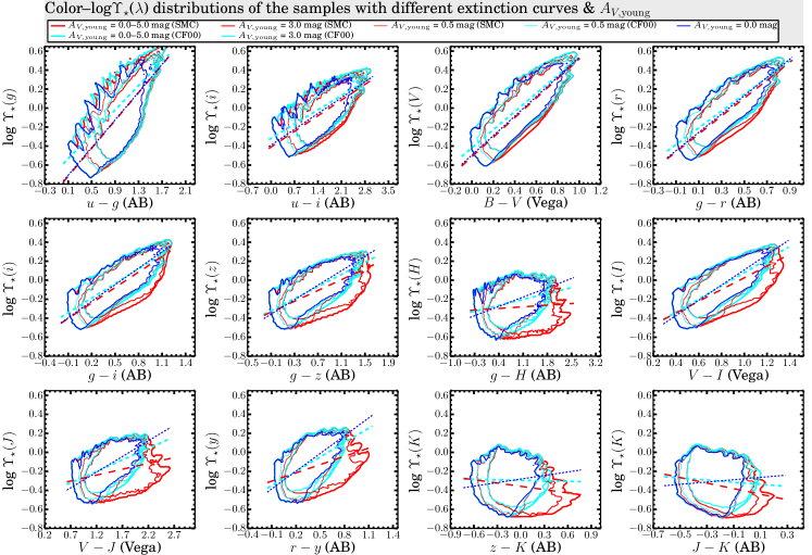
Figure 11.— Effect of dust extinction and dust extinction curves on the color–$\log\Upsilon_{\star}$($\lambda$) distributions of the full samples. Here our default samples are expanded in parameter coverage of $A_{V,{\rm young}}$ by adopting a range of $A_{V,{\rm young}}$ from 0 to 5 mag (with a 0.25 mag step size), and they are also expanded by adopting the relatively shallow CF00 dust extinction curve. The contours in each panel enclose the distributions of the samples with different ranges of $A_{V,{\rm young}}$ and/or dust extinction curves of different slopes, as indicated in the figure title. The SMC-type dust extinction curve has a power-law index of $\simeq$ $-1.2$ in the optical wavelength range, while the CF00 extinction curve has a power-law index of $-0.7$. In each panel, the blue dotted line represents the linear least-squares regression to the full samples generated with $A_{V,{\rm young}}$ = 0.0 mag, and the short-dashed cyan line and long-dashed red line respectively represents the linear regression to the full samples resulting from CF00 and SMC-type dust extinction curves, respectively, with a variable $A_{V,{\rm young}}$ of 0 – 5 mag.

V. $\Upsilon_{\star}$($\lambda$) Estimation with Weighted Ages, Metallicities and Colors

As is found in this work, $\langle{\rm age}\rangle_{\rm\lambda}$ and $\langle{\rm[M/H]}\rangle_{\rm\lambda}$ of composite stellar populations are probably the closest analogs to ages and metallicities of SSPs, as far as the color–$\log\Upsilon_{\star}$($\lambda$) relations are concerned. In particular, $\Upsilon_{\star}$($\lambda$) has the strongest correlation with $\langle{\rm age}\rangle_{\rm\lambda}$. For our default full sample, the Spearman’s rank correlation coefficients $r_{s}$ between $\langle{\rm age}\rangle_{\rm\lambda}$ and $\Upsilon_{\star}$($\lambda$) peak at 0.96 for the $y$ and $J$ bands and decrease toward both shorter- and longer-wavelength passbands (0.88 for $g$, 0.94 for $M$). Ignoring variations of chemical abundance patterns, ages and metallicities are the two parameters that uniquely determine $\Upsilon_{\star}$($\lambda$) of SSPs. Then the question is, to what extent can the $\langle{\rm age}\rangle_{\rm\lambda}$ and $\langle{\rm[M/H]}\rangle_{\rm\lambda}$ constrain $\Upsilon_{\star}$($\lambda$) of galaxies with a wide diversity of SFHs? Understanding the limitation of $\langle{\rm age}\rangle_{\rm\lambda}$, $\langle{\rm[M/H]}\rangle_{\rm\lambda}$, and colors in constraining $\Upsilon_{\star}$($\lambda$) is particularly important, because they are the relevant parameters for planing future observing campaigns and fundamental physical observables that can be readily obtained from spectroscopic or photometric observations.

V.1. SFHs with Associated Metallicity Evolution

The uncertainties of the $\log\Upsilon_{\star}$($\lambda$) estimates, as quantified as the maximum of the half max–min ranges of $\log\Upsilon_{\star}$($\lambda$) within given small intervals of the relevant parameter values, in different passbands are shown in Figure 12 (see the caption for details). With $\langle{\rm age}\rangle_{\rm\lambda}$ alone, $\log\Upsilon_{\star}$($\lambda$) in $J$ band is predicted with an uncertainty of $\simeq$ 0.12 dex, and the uncertainties increase up to 0.25 in the $g$ band and 0.16 in the $M$ band. With additional constraints from $\langle{\rm[M/H]}\rangle_{\rm\lambda}$, the estimation of $\log\Upsilon_{\star}$($\lambda$) improves for all passbands, with the degree of improvement being larger for passbands either longer or shorter than $z$ or $y$. A stronger sensitivity to $\langle{\rm age}\rangle_{\rm\lambda}$ and a weaker sensitivity to $\langle{\rm[M/H]}\rangle_{\rm\lambda}$ for $\Upsilon_{\star}$($\lambda$) of passbands around the boundary between optical and NIR wavelength ranges are analogous to similar findings for SSPs (Worthey 1994). $\langle{\rm age}\rangle_{\rm\lambda}$ and $\langle{\rm[M/H]}\rangle_{\rm\lambda}$ together predict $\log\Upsilon_{\star}$($\lambda$) with uncertainties of $\simeq$ 0.10 dex for $J$ and longer-wavelength passbands, while shortward of $J$, the uncertainties become larger at shorter-wavelength passbands. We note that the uncertainties reported in Figure 12 remain about the same if, say, 2$\times$ smaller binning sizes for $\langle{\rm age}\rangle_{\rm\lambda}$ and $\langle{\rm[M/H]}\rangle_{\rm\lambda}$ are used.

Therefore, at a given $\langle{\rm age}\rangle_{\rm\lambda}$ and $\langle{\rm[M/H]}\rangle_{\rm\lambda}$, the scatter of $\log\Upsilon_{\star}$($\lambda$) induced by the diversity of SFHs and metallicity evolution histories are on the order of $\lesssim$ 0.10 dex for $J$ and longer-wavelength passbands, and the induced scatter becomes increasingly larger toward shorter-wavelength passbands. In particular, the scatter in $g$ band is nearly 2$\times$ larger than in NIR. By adding an additional constraint from $\langle{\rm age}\rangle_{\rm mass}$, the estimation of $\log\Upsilon_{\star}$($\lambda$) improves by $\sim$ 0.03 dex for nearly all passbands. The dependence of $\log\Upsilon_{\star}$($\lambda$) on $\langle{\rm age}\rangle_{\rm mass}$ for given $\langle{\rm age}\rangle_{\rm\lambda}$ and $\langle{\rm[M/H]}\rangle_{\rm\lambda}$ is further demonstrated in Figure 13, whereby one can see a negative correlation between $\log\Upsilon_{\star}$($\lambda$) and $\langle{\rm age}\rangle_{\rm mass}$, especially at relatively young $\langle{\rm age}\rangle_{\rm\lambda}$. This negative correlation indicates that $\langle{\rm age}\rangle_{\rm mass}$ can induce systematic uncertainties to the $\log\Upsilon_{\star}$($\lambda$) estimation of up to $\sim$ 0.2 dex. No single color is particularly sensitive to $\langle{\rm age}\rangle_{\rm mass}$ in general. However, at a given $\langle{\rm age}\rangle_{\rm\lambda}$ and $\langle{\rm[M/H]}\rangle_{\rm\lambda}$, colors have negative correlations with $\langle{\rm age}\rangle_{\rm mass}$ (e.g. Figure 14). By combining $\langle{\rm age}\rangle_{\rm\lambda}$, $\langle{\rm[M/H]}\rangle_{\rm\lambda}$ and colors, $\log\Upsilon_{\star}$($\lambda$) can be constrained with uncertainties (bottom panel of Figure 12) similar to that by $\langle{\rm age}\rangle_{\rm\lambda}$, $\langle{\rm[M/H]}\rangle_{\rm\lambda}$ and $\langle{\rm age}\rangle_{\rm mass}$. We point out that various optical colors perform similarly well in this regard.

The above discussion concerns the ideal cases where $\log\Upsilon_{\star}$($\lambda$) can be estimated through $\langle{\rm age}\rangle_{\rm\lambda}$ and $\langle{\rm[M/H]}\rangle_{\rm\lambda}$ in the relevant passbands. However, in practice, $\langle{\rm age}\rangle_{\rm\lambda}$ and $\langle{\rm[M/H]}\rangle_{\rm\lambda}$ are usually estimated only for a limited wavelength range. For example, people usually use the standard Lick indices (e.g. Worthey et al. 1994) defined in the optical wavelength range to estimate (light-weighted) ages and metallicities. The few Lick indices with the strongest sensitivities to ages (e.g. H$\beta$) and metallicities (e.g. Fe5270, Fe5335, Mg₂) are mainly located in the wavelength range covered by the $g$ band. Figure 12 also shows the uncertainties (in red colors) of $\log\Upsilon_{\star}$($\lambda$) as predicted solely by $g$-band light-weighted ages $\langle{\rm age}\rangle_{g}$ and metallicities $\langle{\rm[M/H]}\rangle_{g}$. Compared to using $\langle{\rm age}\rangle_{\rm\lambda}$ and $\langle{\rm[M/H]}\rangle_{\rm\lambda}$, the uncertainties of $\log\Upsilon_{\star}$($\lambda$) estimation increase by as much as $\sim$ 0.05 dex for longer-wavelength passbands. At a given $\langle{\rm age}\rangle_{g}$ and $\langle{\rm[M/H]}\rangle_{g}$, the scatter of $\log\Upsilon_{\star}$($\lambda$) induced by the diversity of SFHs and metallicity evolution histories is on the order of $\lesssim$ 0.15 dex for passbands with wavelengths longward of $g$. It is worth pointing out that, by using $\langle{\rm age}\rangle_{g}$ and $\langle{\rm[M/H]}\rangle_{g}$, the advantage of NIR over shorter-wavelength passbands (e.g. $V$) in stellar mass estimation becomes very weak ($\sim$ 0.01 – 0.03 dex).

V.2. Monometallic SFHs

The panels on the right-hand side of Figure 12 show the expected uncertainties of $\log\Upsilon_{\star}$($\lambda$) estimates with $\langle{\rm age}\rangle_{\rm\lambda}$, $\langle{\rm[M/H]}\rangle_{\rm\lambda}$, and colors, in the context of monometallic SFHs. Here [M/H] of each individual monometallic SFH in our sample is fixed to the $V$-band light-weighted [M/H], i.e. $\langle{\rm[M/H]}\rangle_{V}$, as determined from our default multimetallic “version” of SFHs. Note that the results, including the values annotated in Figure 12, do not depend on how we set [M/H] of the monometallic SFHs.

Compared to the cases of multimetallic SFHs discussed above, $\langle{\rm age}\rangle_{\rm\lambda}$ predicts $\log\Upsilon_{\star}$($\lambda$) to very similar accuracies. By including additional constraints from $\langle{\rm[M/H]}\rangle_{\rm\lambda}$, $\langle{\rm age}\rangle_{\rm mass}$, or colors, the uncertainties of $\log\Upsilon_{\star}$($\lambda$) estimates are also very similar to those of the multimetallic cases for $J$ and longer wavelength passbands, but shortward of $J$, the uncertainties of $\log\Upsilon_{\star}$($\lambda$), which are about the same as those in $J$ and longer-wavelength passbands, are $\sim$ 2$\times$ smaller than that in the multimetallic cases. By combining $\langle{\rm age}\rangle_{\rm\lambda}$, [M/H], and colors, the uncertainties of $\log\Upsilon_{\star}$($\lambda$) estimates are well below 0.10 dex in all but the $M$ bands, and the uncertainties are actually larger in the NIR passbands than the optical passbands.

Therefore, by using monometallic SFH models to interpret $\langle{\rm age}\rangle_{g}$ and $\langle{\rm[M/H]}\rangle_{g}$ determined from optical spectra of real galaxies, one tends to underestimate the uncertainties of $\log\Upsilon_{\star}$($\lambda$) by $\lesssim$ 0.1 dex for the optical passbands and $\lesssim$ 0.05 dex for the NIR passbands.

V.3. Scatter Induced by Dust Extinction and Reddening

The above two subsections concern the uncertainties of $\log\Upsilon_{\star}$($\lambda$) estimates induced by SFHs and metallicity evolution. Here we explore the additional uncertainties induced by a variable $A_{V,{\rm young}}$, under the assumption of an SMC-bar dust extinction curve that has a larger influence on color–$\log\Upsilon_{\star}$($\lambda$) distributions than shallower ones (Section IV.5).

Like in Figure 12, the results for the samples expanded with variable $A_{V,{\rm young}}$ from 0 to 5 mag are shown in Figure 15. If $\langle{\rm age}\rangle_{\rm\lambda}$ and $\langle{\rm[M/H]}\rangle_{\rm\lambda}$ are invoked to estimate $\log\Upsilon_{\star}$($\lambda$) for the case of variable $A_{V,{\rm young}}$, $\log\Upsilon_{\star}$($\lambda$) can be constrained with uncertainties very similar to those of the low dust extinction case. Nevertheless, if $\langle{\rm age}\rangle_{g}$ and $\langle{\rm[M/H]}\rangle_{g}$ are used, $\log\Upsilon_{\star}$($\lambda$) estimation is subject to uncertainties of $\gtrsim$ 0.20 dex for nearly all passbands, and the uncertainties for the NIR passbands are slightly larger than those for the optical passbands.

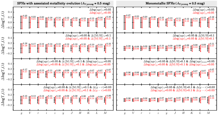
Figure 12.— Maximum of half max–min ranges of $\log\Upsilon_{\star}$($\lambda$) constrained by light-weighted ages $\langle{\rm age}\rangle_{\rm\lambda}$, light-weighted metallicities $\langle{\rm[M/H]}\rangle_{\rm\lambda}$, $\langle{\rm age}\rangle_{\rm mass}$, and ($g$$-$$r$) colors. The panels on the left-hand side are for the SFHs of the full sample with associated metallicity evolution, while the panels on the right-hand side are for monometallic SFHs of the full sample with [M/H] fixed to their respective $V$-band light-weighted [M/H]. From the top to bottom panels, the results are constrained by log$\langle{\rm age}\rangle_{\rm\lambda}$ (0.05 dex intervals); by log$\langle{\rm age}\rangle_{\rm\lambda}$ and $\langle{\rm[M/H]}\rangle_{\rm\lambda}$ (0.05$\times$0.1 dex intervals); by log$\langle{\rm age}\rangle_{\rm\lambda}$, $\langle{\rm[M/H]}\rangle_{\rm\lambda}$, and log$\langle{\rm age}\rangle_{\rm mass}$ (0.05$\times$0.1$\times$0.05 dex intervals); and by log$\langle{\rm age}\rangle_{\rm\lambda}$, $\langle{\rm[M/H]}\rangle_{\rm\lambda}$, and ($g$$-$$r$) colors (0.05$\times$0.1$\times$0.03 intervals). In each panel, the black symbols represent results as constrained by light-weighted parameters in passbands $\lambda$ indicated by the x-axis tick labels, while the red symbols illustrate the corresponding results as constrained by $g$-band light-weighted parameters. The numerical values of $\Delta$$\log\Upsilon_{\star}$($\lambda$) are shown as labels correspondingly. See Section V for discussions.

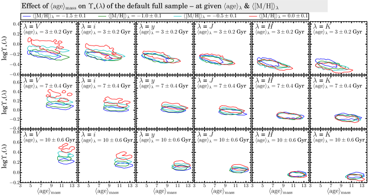
Figure 13.— Effect of $\langle{\rm age}\rangle_{\rm mass}$ on $\log\Upsilon_{\star}$($\lambda$), at given $\langle{\rm age}\rangle_{\rm\lambda}$ and $\langle{\rm[M/H]}\rangle_{\rm\lambda}$. Here the effect is illustrated for several representative passbands as indicated in the figure. See Section V for discussions.

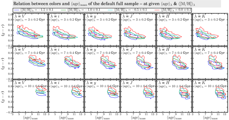
Figure 14.— Relation between ($g$$-$$r$) and $\langle{\rm age}\rangle_{\rm mass}$ at given $\langle{\rm age}\rangle_{\rm\lambda}$ and $\langle{\rm[M/H]}\rangle_{\rm\lambda}$. Here the effect is illustrated for $\langle{\rm age}\rangle_{\rm\lambda}$ and $\langle{\rm[M/H]}\rangle_{\rm\lambda}$ in several representative passbands as indicated in the figure. See Section V for discussions.

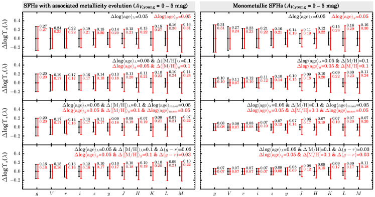
Figure 15.— Same as Figure 12, but for our full samples expanded with variable $A_{V,{\rm young}}$ ranging from 0.0 to 0.5 mag. See Section V for discussions.

V.4. The Optimal Passbands and Colors for $\Upsilon_{\star}$($\lambda$) Estimates

V.4.1 The Optimal Single Passbands

As shown in Figure 16, $\log\Upsilon_{\star}$($\lambda$) of the $J$ and $H$ bands have the smallest half max–min ranges $\Delta$$\log\Upsilon_{\star}$($\lambda$) ($\simeq$ 0.35 dex) among all passbands, regardless of dust extinction. Passbands longward and shortward of $JH$ have progressively larger $\Delta$$\log\Upsilon_{\star}$($\lambda$). As noted in previous sections, $\log\Upsilon_{\star}$($\lambda$) of passbands with wavelength around the $J$ band show the strongest sensitivities to $\langle{\rm age}\rangle_{\rm\lambda}$ and the weakest sensitivities to $\langle{\rm[M/H]}\rangle_{\rm\lambda}$, while $\log\Upsilon_{\star}$($\lambda$) of passbands at either longer or shorter wavelengths have increasingly larger sensitivities to $\langle{\rm[M/H]}\rangle_{\rm\lambda}$ and smaller sensitivities to $\langle{\rm age}\rangle_{\rm\lambda}$. Although we do not deal with systematic uncertainties inherent in stellar evolution models in this work, it is worth emphasizing that modeling of NIR emission from stellar populations of several hundred Myr to $\sim$ 3 Gyr is subject to substantial uncertainties, due to our poor knowledge of the TP-AGB phase of stellar evolution.

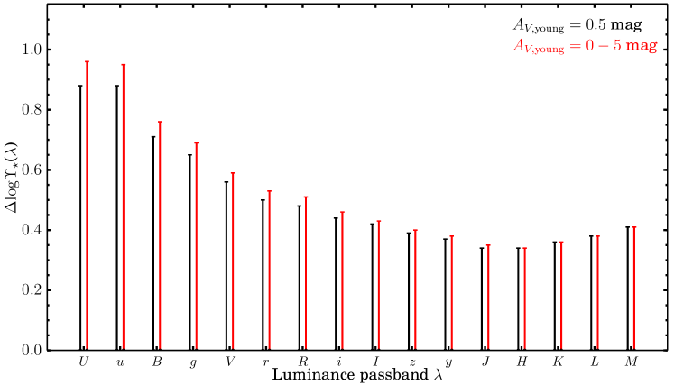
Figure 16.— Half max–min ranges of $\log\Upsilon_{\star}$($\lambda$) of different passbands. Results for our default full sample of $A_{V,{\rm young}}$ = 0.5 mag (black) and the full samples with variable $A_{V,{\rm young}}$ ranging from 0.0 to 5.0 mag (red) are shown separately. 

V.4.2 The Optimal Single color–$\log\Upsilon_{\star}$($\lambda$) Relations

Color–$\log\Upsilon_{\star}$($\lambda$) correlations help to reduce the uncertainties of $\log\Upsilon_{\star}$($\lambda$) estimation for all passbands. Figure 17 shows the median and maximum $\Delta$$\log\Upsilon_{\star}$($\lambda$) of various passbands $\lambda$ in 0.03 mag single-color intervals of our default full sample with $A_{V,{\rm young}}$ = 0.5 mag. Likewise, Figure 18 shows the results for the full sample with variable $A_{V,{\rm young}}$. Compared to the cases without color information (Section V.4.1), single colors help to reduce systematic uncertainties in the $\log\Upsilon_{\star}$($\lambda$) estimation by factors of $\sim$ 1.6 – 2.5 for the sample with $A_{V,{\rm young}}$ fixed to 0.5 mag and of $\sim$ 1.3 – 2.2 for the samples with variable $A_{V,{\rm young}}$. In particular, $\log\Upsilon_{\star}$($\lambda$) of passbands shortward of $H$ can generally be better constrained by single colors than that of longer-wavelength passbands. For given $\log\Upsilon_{\star}$($\lambda$), colors covering longer wavelength baselines toward the blue end, preferably $B$ or $g$, generally offer tighter constraints on $\log\Upsilon_{\star}$($\lambda$) than the others.

Taking $\Delta$$\log\Upsilon_{\star}$($\lambda$) reported in Figures 17 and 18 at face value, $\log\Upsilon_{\star}$($i$) can be constrained with the smallest half max–min ranges by using the ($g$$-$$i$) color. However, $\log\Upsilon_{\star}$($\lambda$) of other passbands, such as $J$, $y$, $z$, $r$ and $V$, can be constrained with very similar $\Delta$$\log\Upsilon_{\star}$($\lambda$) (within $\sim$ 0.01 dex). We note that ($g$$-$$i$) is the preferred color for $\Upsilon_{\star}$ estimation by Z09. Gallazzi & Bell (2009) reached a similar conclusion that ($g$$-$$i$) offers the tightest constraint on $\Upsilon_{\star}$($z$). Nevertheless, $\Upsilon_{\star}$($\lambda$) of longer-wavelength passbands are subject to larger systematic uncertainties induced by SFHs (e.g. $\langle{\rm age}\rangle_{\rm\lambda}$, $\langle{\rm age}\rangle_{\rm mass}$), and color–$\log\Upsilon_{\star}$($\lambda$) relations (e.g. slopes and intercepts) defined by colors covering longer-wavelength baselines are subject to larger systematic influences from metallicities, dust extinction and reddening (Sections IV.3 and IV.5). The linear slopes and intercepts of ($g$$-$$r$)–$\log\Upsilon_{\star}$($r$) and especially ($B$$-$$V$)–$\log\Upsilon_{\star}$($V$) relations have the weakest dependencies on $\langle{\rm age}\rangle_{\rm\lambda}$, $\langle{\rm[M/H]}\rangle_{\rm\lambda}$, $\langle{\rm age}\rangle_{\rm mass}$, dust extinction, and reddening and thus are the optimal choices for a least-biased estimation of $\Upsilon_{\star}$($\lambda$), if no additional constraints on SFHs and metallicities are available. It is noteworthy that, for our samples with variable $A_{V,{\rm young}}$, the difference between median $\Delta$$\log\Upsilon_{\star}$($V$) as estimated by ($B$$-$$V$) and median $\Delta$$\log\Upsilon_{\star}$($i$) as estimated by ($g$$-$$i$) is only $\simeq$ 0.02 dex.

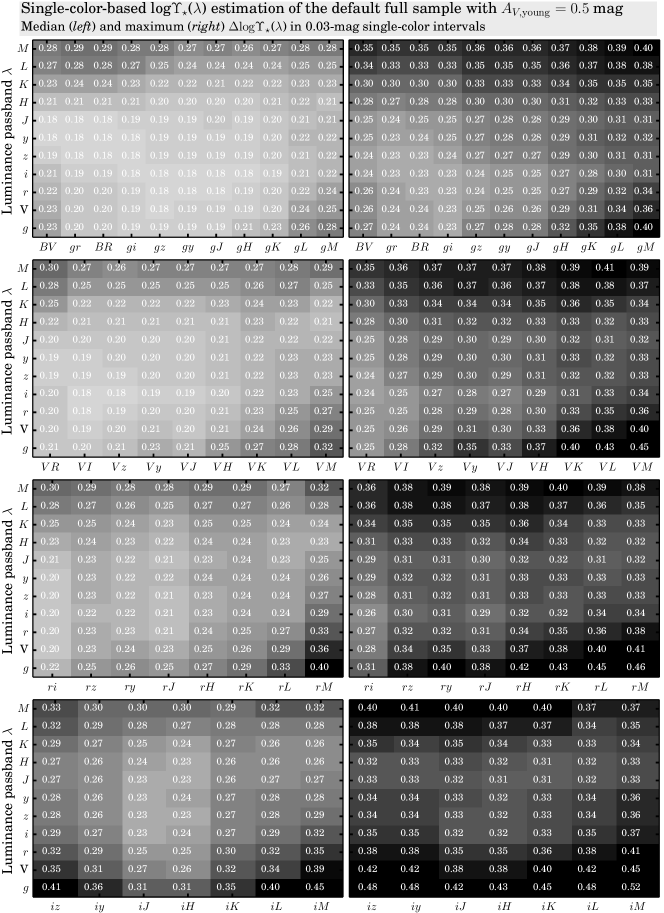
Figure 17.— Uncertainties of $\log\Upsilon_{\star}$($\lambda$) estimated by one single color for the our default full sample, with $A_{V,{\rm young}}$ = 0.5 mag. Colors are labeled on the x axes, and the luminance passband $\lambda$ are labeled on the y axes. The uncertainties $\Delta$$\log\Upsilon_{\star}$($\lambda$) are quantified as either the median (left panels) or maximum (right panels) of the half max–min ranges of $\log\Upsilon_{\star}$($\lambda$) in 0.03 mag color intervals. $\Delta$$\log\Upsilon_{\star}$($\lambda$) is represented in gray scale (larger $\Delta$$\log\Upsilon_{\star}$($\lambda$) are represented with darker gray scales) and is also annotated correspondingly in each cell.

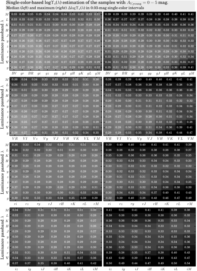
Figure 18.— Same as Figure 17, but for the full samples with $A_{V,{\rm young}}$ ranging from 0.0 to 5.0 mag.

V.4.3 The Optimal Combinations of Two Colors

$\Upsilon_{\star}$($\lambda$) can be better constrained with more than one color. As examples, Figure 19 shows the color-dependent improvement of $\log\Upsilon_{\star}$($i$) estimation by combining a second optical–optical ($r$$-$$i$) or an optical–NIR ($i$$-$$K$) color with the ($g$$-$$i$)–$\log\Upsilon_{\star}$($i$) relations. The half max–min ranges of $\log\Upsilon_{\star}$($i$) $\Delta$$\log\Upsilon_{\star}$($i$) are generally reduced when ($r$$-$$i$) or especially ($i$$-$$K$) is included, and the degree of improvement is generally larger toward either the bluer or redder edges of colors. The efficacy of a second color is further illustrated in Figure 20, where the distributions of galaxies with different ($r$$-$$i$) or ($i$$-$$K$) color values are distinguished on the ($g$$-$$i$)–$\log\Upsilon_{\star}$($i$) planes. At a low dust extinction of $A_{V,{\rm young}}$ = 0.5 mag (left panels of Figure 20), the iso-($i$$-$$K$) contours largely follow that of the $i$-band light-weighted [M/H] (Figure 9) on the ($g$$-$$i$)–$\log\Upsilon_{\star}$($i$) planes, suggesting that the effect of an additional optical–NIR color is to partially remove the dependence of $\log\Upsilon_{\star}$($i$) on [M/H]. Due to the age-metallicity degeneracy, galaxies with older $\langle{\rm age}\rangle_{\rm\lambda}$ tend to have smaller $\langle{\rm[M/H]}\rangle_{\rm\lambda}$ for given color values. Therefore, by partially removing the [M/H] dependence, optical–NIR colors help to improve the constraints on $\langle{\rm age}\rangle_{\rm\lambda}$ and thus $\log\Upsilon_{\star}$($\lambda$). On the other hand, at high dust extinctions (e.g. right panels of Figure 20), galaxies with higher dust extinction have on average redder optical-NIR colors for given optical color values, so optical–NIR colors help to partially remove the positive dependence of $\log\Upsilon_{\star}$($\lambda$) on dust extinction.

To be complete, we determine the median and maximum $\Delta$$\log\Upsilon_{\star}$($\lambda$) predicted by various pairs of colors, and the results are shown in Figures 21 and 22. The combinations of optical–optical and optical–NIR colors covering larger wavelength baselines generally provide tighter constraints on $\log\Upsilon_{\star}$($\lambda$) than the other combinations. $\log\Upsilon_{\star}$($\lambda$) of the samples with variable $A_{V,{\rm young}}$ are constrained with larger uncertainties than that of the sample with a low $A_{V,{\rm young}}$ of 0.5 mag. Nevertheless, the degree of improvement of two colors over single colors for the samples with variable $A_{V,{\rm young}}$ is generally larger than that for the sample with low $A_{V,{\rm young}}$ of 0.5 mag.

$\Upsilon_{\star}$($\lambda$) estimation with an optical–optical plus optical–NIR colors was first extensively studied by Z09. Z09 found that $\Upsilon_{\star}$($\lambda$) estimated with the ($g$$-$$i$)–$\log\Upsilon_{\star}$($i$) relation alone is in excellent agreement with that estimated with the combination of ($g$$-$$i$) and ($i-H$), except for extremely star-forming and/or dust-extincted regions of galaxies. In this work, we have shown that, not just for extremely star-forming and dust-extincted regions, combinations of ($g$$-$$i$) and an optical–NIR color are generally favoured over the ($g$$-$$i$)–$\log\Upsilon_{\star}$($i$) relation alone for a robust $\Upsilon_{\star}$($\lambda$) estimation. In addition, since dust extinction and reddening have a smaller effect on optical color–$\log\Upsilon_{\star}$($\lambda$) distributions for extinction curves shallower than our default SMC-bar extinction curves (Section IV.5), the efficacy of optical–NIR colors for dusty and young populations is reduced for shallower dust extinction curves.

Regarding the role played by an additional optical–NIR color in stellar mass estimation for extremely star-forming regions with relatively low dust extinction, we emphasize that the optical–NIR colors primarily help to partially remove the dependencies of optical color–$\log\Upsilon_{\star}$($\lambda$) distributions on [M/H], rather than (as often taken for granted in the literature) to recover the mass of older stellar populations that are outshined in shorter optical wavelengths by luminosity-dominant younger populations. This interpretation is also in line with the results of Section VI where we will show that the efficacy of NIR passbands in stellar mass estimation is mainly to improve stellar mass estimation at relatively high [M/H].

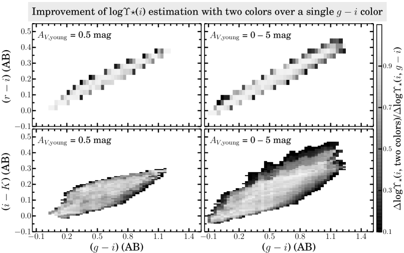
Figure 19.— Improvement of $\log\Upsilon_{\star}$($i$) estimation with combinations of ($g$$-$$i$) and ($r$$-$$i$) (top panels) and of ($g$$-$$i$) and ($i$$-$$K$) (bottom panels) over using a single ($g$$-$$i$) color. The distributions for the samples of $A_{V,{\rm young}}$ = 0.5 mag and of $A_{V,{\rm young}}$ = 0 – 5 mag are shown in the left and right panels respectively. The half max–min ranges of $\Delta$$\log\Upsilon_{\star}$($i$) are determined in each 0.03$\times$0.03 color interval. The gray scales represent the ratios of $\Delta$$\log\Upsilon_{\star}$($i$) from combinations of two colors to $\Delta$$\log\Upsilon_{\star}$($i$) from a single ($g$$-$$i$) color.

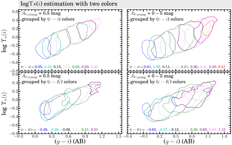
Figure 20.— Distributions of subsamples with different $r$$-$$i$ or $i$$-$$K$ colors on the ($g$$-$$i$)–$\log\Upsilon_{\star}$($i$) planes. The full samples with $A_{V,{\rm young}}$ = 0.5 mag (left panels) and $A_{V,{\rm young}}$ = 0 – 5 mag (right panels) are grouped into different $r$$-$$i$ (top panels) and $i$$-$$K$ (bottom panels) color values. Each contour encloses subsamples within a color interval of 0.05 mag around the values annotated at the bottom of each panel.

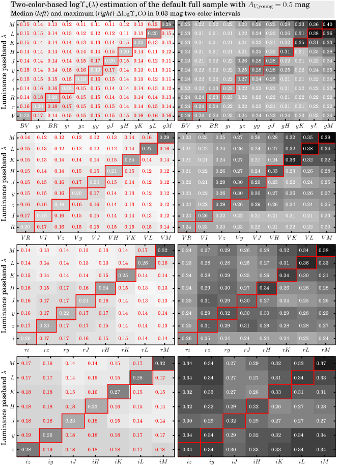
Figure 21.— Uncertainties of $\log\Upsilon_{\star}$($\lambda$) estimated by two colors (except for the cells along the diagonal of each panel) of the our default full sample, with $A_{V,{\rm young}}$ = 0.5 mag. Pairs of passbands as labeled on the x axes, together with passbands $\lambda$ as labeled on the y axes, are used to estimate $\log\Upsilon_{\star}$($\lambda$). The uncertainties $\Delta$$\log\Upsilon_{\star}$($\lambda$) are quantified as either the median (left panels) or maximum (right panels) of the half max-min ranges of $\log\Upsilon_{\star}$($\lambda$). $\Delta$$\log\Upsilon_{\star}$($\lambda$) is represented in gray scale (larger $\Delta$$\log\Upsilon_{\star}$($\lambda$) are represented with darker gray scales) and is also annotated correspondingly in each cell. Note that the text colors, either red or white, are chosen just to increase the contrast with respect to the background for a better readability.

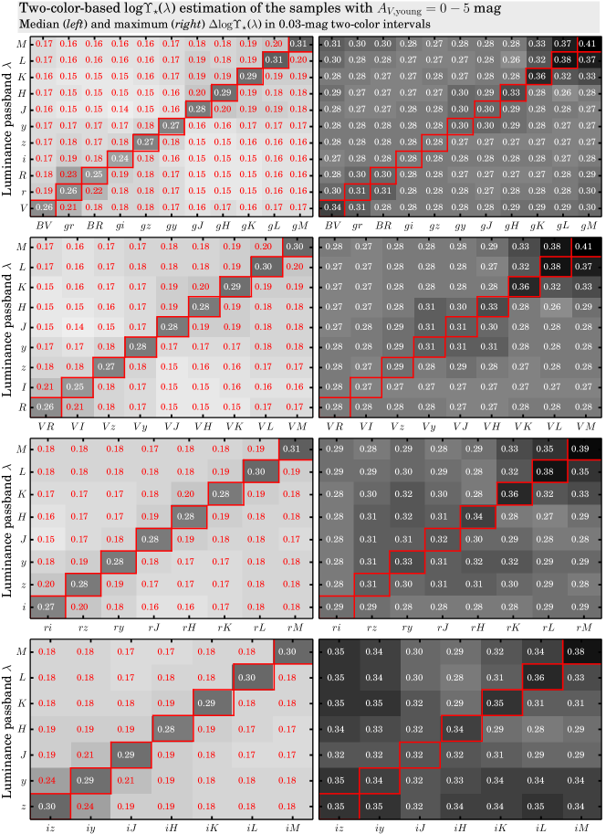
Figure 22.— Same as Figure 21, but for the full samples with $A_{V,{\rm young}}$ ranging from 0 to 5 mag.

VI. Stellar Mass Estimation from the NNLS SED Fitting

Following the procedure described in Section III.2, the broadband SEDs of our default full sample covering a variety of wavelength ranges from FUV to the $M$ band (i.e. FUV, NUV, $u$, $g$, $r$, $i$ ,$z$, $y$, $J$, $H$, $K$, $L$, and $M$) are fitted with the NNLS algorithm. Random “observational” photometric errors of $\sigma_{\rm phot}$ = 0.01 or 0.03 mag are assigned to all passbands involved in the SED fitting. The logarithmic differences between the stellar mass from the SED fitting and the input $\log M_{\star}$(fitting)$-$$\log M_{\star}$(input) as a function of the $g-i$ color are shown in Figures 23 to 30. In particular, results from multimetallic SED fitting with $A_{V,{\rm young}}$ fixed to 0.5 mag are shown in Figures 23 and 24 for $\sigma_{\rm phot}$ = 0.01 mag and 0.03 mag, respectively, results from monometallic SED fitting with $A_{V,{\rm young}}$ fixed to 0.5 mag are shown in Figures 25 and 26 for $\sigma_{\rm phot}$ = 0.01 mag and 0.03 mag, respectively, results from multimetallic SED fitting with $A_{V,{\rm young}}$ being a free parameter are shown in Figures 27 and 28 for $\sigma_{\rm phot}$ = 0.01 mag and 0.03 mag, respectively, and results from monometallic SED fitting with $A_{V,{\rm young}}$ being a free parameter are shown in Figures 29 and 30 for $\sigma_{\rm phot}$ = 0.01 mag and 0.03 mag, respectively. To illustrate the effect of wavelength coverage (i.e. with/without UV and/or NIR) on the recovery accuracy of stellar mass, the results of fitting to the SEDs, from FUV to $M$, from $u$ to $M$, from $g$ to $M$, from FUV to $y$, and from $u$ to $y$, are presented in different columns in the figures.

VI.1. Stellar Mass Estimated from UV-to-NIR or Optical-to-NIR SED Fitting

Multimetallic fitting. By fitting the full FUV-to-$M$ SEDs, stellar masses are recovered with biases (i.e. the vertical extent of the contours above or below 0 in the figures) ranging from $\sim$ $-0.2$ to 0.3 dex over the whole color ranges. Moreover, the uncertainties and biases are smaller at redder optical colors, which is in line with (1) the generally shallower and narrower color–$\log\Upsilon_{\star}$($\lambda$) relations and (2) a higher efficacy of NIR passbands in removing the [M/H] dependence of optical color–$\log\Upsilon_{\star}$($\lambda$) relations at redder colors. By fitting only the optical-to-NIR SEDs, the typical biases of stellar mass estimates, including their trend with colors, are very similar to those from the full SED fitting. The UV-to-NIR or optical-to-NIR SED fitting with $A_{V,{\rm young}}$ being either fixed (= 0.5 mag) or variable results in very similar quality of stellar mass estimation. In addition, increasing the photometric errors from 0.01 to 0.03 mag does not significantly affect the range of biases of stellar mass estimated from the UV-to-NIR or optical-to-NIR SED fitting, but does result in slightly ($\lesssim$ 0.05 dex) larger negative biases at the blue end and larger positive (or negative) biases at the red end when $A_{V,{\rm young}}$ is fixed (or variable) in the SED fitting.

Monometallic fitting. Monometallic SED fitting gives stellar mass estimates with biases ranging from $\sim$ $-0.3$ to 0.15 dex. So monometallic fitting has a stronger tendency (by $\sim$ 0.1 dex on average) of underestimating stellar masses than the multimetallic fitting. We note that, with larger uncertainties of stellar mass estimates than the multimetallic fitting at the red end of colors, monometallic fitting gives more consistent uncertainties and biases across the whole color ranges. Increasing photometric errors of the monometallic fitting has an effect on stellar mass estimation that is very similar to the multimetallic fitting, as described above.

VI.2. Stellar Mass Estimated from SED Fitting without NIR Passbands

Multimetallic fitting. Without passbands longward of $y$, the SED fitting performs progressively worse in stellar mass estimation for shorter-wavelength coverages. In particular, with $A_{V,{\rm young}}$ being fixed, the optical $u$-to-$y$ SED fitting gives stellar mass estimates with biases ranging from $\sim$ $-0.5$ to 0.3 dex (i.e. being negative on average) for $\sigma_{\rm phot}$ = 0.01 mag and from $\sim$ $-0.2$ to 0.4 dex (i.e. being positive on average) for $\sigma_{\rm phot}$ = 0.03 mag. Moreover, with $A_{V,{\rm young}}$ being a free parameter, the optical $u$-to-$y$ SED fitting gives stellar mass estimates with biases ranging from $\sim$ $-0.6$ to $0.2$ dex (i.e. being negative on average) for either $\sigma_{\rm phot}$ = 0.01 mag or 0.03 mag. Therefore, SED fitting with dust extinction as a free fitting parameter has a significantly stronger tendency of underestimating stellar masses if NIR passbands are not used in the fitting. The importance of NIR passbands in stellar mass estimation has been realized by many previous studies (e.g. Lee et al. 2009a; Kannappan & Gawiser 2007; Bolzonella et al. 2010; Pforr et al. 2013; Mitchell et al. 2013).

Monometallic fitting. Similar to the general trend for the full SED fitting discussed above, monometallic fitting without NIR passbands has a stronger tendency of underestimating stellar masses than the corresponding multimetallic fitting.

VI.3. Dependences of Stellar Mass Estimates on Input SFHs and Metallicities

Stellar masses tend to be underestimated at older $\langle{\rm age}\rangle_{\rm mass}$ while overestimated at younger $\langle{\rm age}\rangle_{\rm mass}$. The $\langle{\rm age}\rangle_{\rm mass}$-dependent biases are stronger for SED fitting with fewer passbands, especially when NIR passbands are not used. The aforementioned larger biases of stellar mass estimates at bluer colors are primarily driven by galaxies with relatively smaller $\langle{\rm age}\rangle_{\rm\lambda}$ and higher $\langle{\rm[M/H]}\rangle_{\rm\lambda}$. It is noteworthy that the optical-to-NIR fitting has a stronger tendency of overestimating stellar masses at the youngest $\langle{\rm age}\rangle_{\rm\lambda}$ than the UV-to-NIR fitting. Moreover, we also note that the worse performance of SED fitting without NIR passbands as mentioned above is primarily driven by galaxies with higher $\langle{\rm[M/H]}\rangle_{\rm\lambda}$.

The $\langle{\rm age}\rangle_{\rm mass}$-dependent biases suggest that, as with single colors, broadband SED fitting is generally not sensitive to $\langle{\rm age}\rangle_{\rm mass}$, and the most probable stellar mass estimates from SED fitting are just the median over SFHs with all possible ranges of $\langle{\rm age}\rangle_{\rm mass}$ for given SEDs. In addition, the apparently larger biases of stellar mass estimates at higher $\langle{\rm[M/H]}\rangle_{\rm\lambda}$ reflect the generally broader and steeper color–$\log\Upsilon_{\star}$($\lambda$) relations at higher $\langle{\rm[M/H]}\rangle_{\rm\lambda}$  (Section IV.4.1), rather than a poorer (or better) performance of SED fitting at higher (or lower) $\langle{\rm[M/H]}\rangle_{\rm\lambda}$. If the NIR passbands are used in SED fitting, the dependence of uncertainties and biases on $\langle{\rm[M/H]}\rangle_{\rm\lambda}$ can be partially removed.

VI.4. Why Monometallic SED fitting Tends to Underestimate Stellar Masses?

In a multimetallic SED fitting, SEDs with slightly bluer colors can be fitted by giving more weights to either younger SSP components of relatively high metallicities (leading to younger $\langle{\rm age}\rangle_{\rm\lambda}$) or older SSP components of relatively low metallicities (leading to older $\langle{\rm age}\rangle_{\rm\lambda}$), whereas in a monometallic SED fitting, SEDs with slightly bluer colors can only be fitted by giving more weights to younger SSP components (leading to younger $\langle{\rm age}\rangle_{\rm\lambda}$). Since $\Upsilon_{\star}$($\lambda$) is positively correlated with $\langle{\rm age}\rangle_{\rm\lambda}$, the monometallic SED fitting has a stronger tendency of underestimating stellar masses of real galaxies.

Gallazzi & Bell (2009) also explored the uncertainties of stellar mass estimation induced by using monometallic models to fit mock galaxies with multimetallic exponentially declining SFHs. They found that stellar masses tend to be underestimated (or overestimated) for their old (or young) galaxies when single $g-i$ colors are used to fit monometallic models to multimetallic input SFHs. The average trend of either overestimation or underestimation of stellar masses found by Gallazzi & Bell (2009) is inevitably influenced by their prior assumptions on the SFH libraries. However, they found that mass estimates are barely affected when using the two age-sensitive stellar absorption features D4000_n and H$\delta_{A}$, instead of $g-i$ colors, in the fitting. This is consistent with a tighter constraint on light-weighted ages and thus $\Upsilon_{\star}$ offered by the two spectral features.

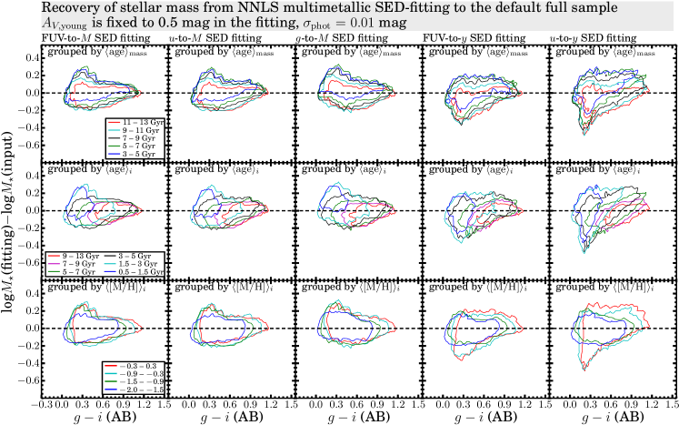
Figure 23.— Recovery of the input stellar masses of our default full sample through NNLS SED fitting, where $A_{V,{\rm young}}$ is fixed to 0.5 mag. The logarithmic differences between the stellar mass from NNLS SED fitting and the input are plotted as a function of the $g$$-$$i$ color. From the top to bottom panels, the distributions of data points are grouped by $\langle{\rm age}\rangle_{\rm mass}$ (top), $i$-band light-weighted ages (middle), and $i$-band light-weighted [M/H]. From the left to right panels, the results of fitting to the full SEDs from FUV to $M$, from $u$ to $M$, from $g$ to $M$, from FUV to $y$, and from $u$ to $y$ are shown. Photometric errors of $\sigma_{\rm phot}$ = 0.01 mag are assigned to all passbands for SED fitting. 

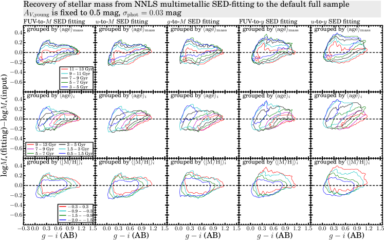
Figure 24.— Same as Figure 23, except that the photometric errors $\sigma_{\rm phot}$ = 0.03 mag.

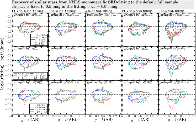
Figure 25.— Same as Figure 23, except that the monometallic SSP templates are used for SED fitting.

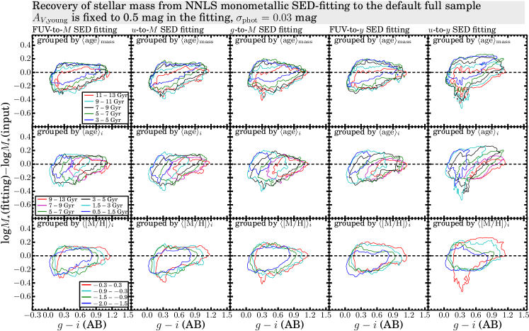
Figure 26.— Same as Figure 24, except that the monometallic SSP templates are used for SED fitting.

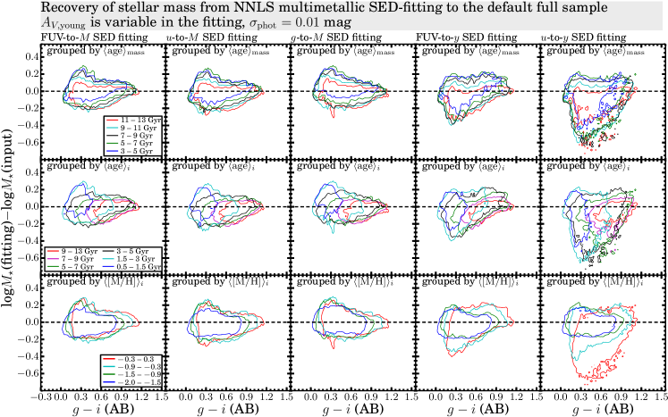
Figure 27.— Same as Figure 23, except that the dust extinction $A_{V,{\rm young}}$ is a free parameter in the SED fitting.

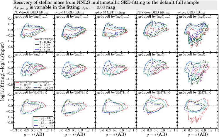
Figure 28.— Same as Figure 24, except that the dust extinction $A_{V,{\rm young}}$ is a free parameter in the SED fitting.

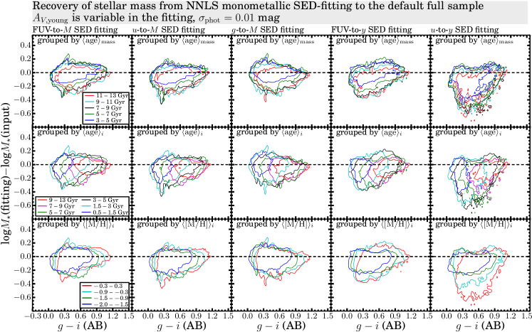
Figure 29.— Same as Figure 25, except that the dust extinction $A_{V,{\rm young}}$ is a free parameter in the SED fitting.

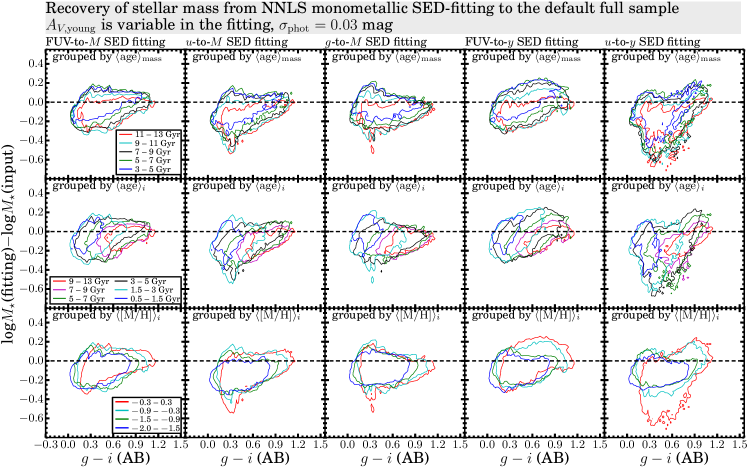
Figure 30.— Same as Figure 26, except that the dust extinction $A_{V,{\rm young}}$ is a free parameter in the SED fitting.

VII. Discussion

VII.1. Origin of the Discrepancies between color–$\log\Upsilon_{\star}$($\lambda$) Relations Calibrated by Different Studies

In light of our study of the color–$\log\Upsilon_{\star}$($\lambda$) distributions in this work, here we try to address the reason behind the discrepancies between various color–$\log\Upsilon_{\star}$($\lambda$) relations from previous studies. We focus on the four most commonly studied and tightest optical color–$\log\Upsilon_{\star}$($\lambda$) distributions, i.e. ($B$$-$$V$)–$\log\Upsilon_{\star}$($V$), ($g$$-$$r$)–$\log\Upsilon_{\star}$($r$), ($g$$-$$i$)–$\log\Upsilon_{\star}$($i$), and ($g$$-$$z$)–$\log\Upsilon_{\star}$($z$). Since most of the color–$\log\Upsilon_{\star}$($\lambda$) relations available in the literature were calibrated based on the BC03 models, in this subsection different literature calibrations are confronted with the distributions of our default full sample of $A_{V,{\rm young}}$ = 0.5 mag (Figure 31), computed with the BC03 SSP models. We emphasize that the results based on the BC03 models are in general agreement with those based on the FSPS models.

The color–$\log\Upsilon_{\star}$($\lambda$) distributions shown in Figure 31 are grouped by $\langle{\rm age}\rangle_{\rm mass}$ and $\langle{\rm age}\rangle_{\lambda,{\rm long}}$ in the upper and lower panels respectively. $\langle{\rm age}\rangle_{\rm mass}$ and $\langle{\rm age}\rangle_{\lambda,{\rm long}}$ are the two key parameters that differentiate the full sample into groups that follow distinctly different optical color–$\log\Upsilon_{\star}$($\lambda$) correlations (Section IV.3). The overplotted literature color–$\log\Upsilon_{\star}$($\lambda$) relations are as in Figure 3. These relations are based on either the original or the updated but unpublished 2007 version of BC03 models (Charlot & Bruzual 2007; hereafter CB07). The CB07 models are different from the original BC03 models primarily in a $\gtrsim$ 2$\times$ enhanced NIR luminosity contribution at intermediate ages from the TP-AGB evolutionary phases, following Marigo & Girardi (2007) and Marigo et al. (2008). Among the overplotted color–$\log\Upsilon_{\star}$($\lambda$) relations, the Z09 and H16 relations are based on the CB07 models, and the T11 and R15 relations are based on the BC03 models. The most commonly used B03 relations were calibrated with the PEGASE models, which are based on the same Padova (1994) isochrones as the BC03 models. The R15 relations plotted here are the ones predicted by the BC03 version of the MAGPHYS SED fitting package (da Cunha et al. 2008), and the Z09 relations are based on SFH libraries constructed by adopting very similar prior constraints to those of MAGPHYS. Hence, it is no surprise that the R15 and Z09 relations have about the same slopes, and the discrepancies of the their zero points (or intercepts) are smaller for colors involving shorter-wavelength passbands that are less influenced by the different treatment of TP-AGB phases between the BC03 and CB07 models. In addition, except for the B03 relations, all of the other relations are calibrated with the Chabrier (2003) IMF. To make a fair comparison with others, we have reduced, in Figures 3 and 31, the zero points of the B03 relations by 0.12 dex to transform from a diet-Salpeter IMF, used in B03, to a Chabrier (2003) IMF.

As shown in Figure 31, the discrepancies between different relations are smaller for color–$\log\Upsilon_{\star}$($\lambda$) distributions covering shorter-wavelength baselines, with ($B$$-$$V$)–$\log\Upsilon_{\star}$($V$) being the one with the smallest discrepancies and ($g$$-$$z$)–$\log\Upsilon_{\star}$($z$) being the one with the largest discrepancies. This is in line with our finding that the linear slopes and intercepts of the ($B$$-$$V$)–$\log\Upsilon_{\star}$($V$) relations are least influenced by SFHs, metallicities, and dust extinction/reddening. As pointed out in Section V.4.2, color–$\log\Upsilon_{\star}$($\lambda$) relations involving $\log\Upsilon_{\star}$($V$) and colors covering wavelength baselines longer than $B$$-$$V$, such as $g$$-$$i$, are subject to larger systematic uncertainties induced by metallicities and dust reddening. This explains the finding of McGaugh & Schombert (2014) that, for the same galaxy, $\Upsilon_{\star}$($\lambda$) estimated (through the $B$$-$$V$ color) with color–$\log\Upsilon_{\star}$($\lambda$) relations calibrated by different studies agree closely in the $V$ band but diverge at longer wavelengths.

VII.2. Comments on Linear color–$\log\Upsilon_{\star}$($\lambda$) Relations in the Literature

Before proceeding to comment on the individual color–$\log\Upsilon_{\star}$($\lambda$) relations, we briefly summarize the key assumptions of SFH models adopted by different studies. The B03 relations are based on SED fitting with libraries of single exponential SFHs ($\propto$ $\exp(-t/\tau)$), with the $e$-folding timescale $\tau$ being a free parameter and the time $t$ since the SFHs commenced being fixed to 12 Gyr. The T11 relations are also based on single exponential SFH libraries, with both $t$ and $\tau$ being free parameters. The Z09 and R15 relations are determined by adding random bursts on top of single exponential SFHs, with $t$ and $\tau$ being free parameters. The H16 relations are determined with a library of SFHs (Zhang et al. 2012) that is constructed by approximating the galaxy lifetime (i.e. 14 Gyr) with 6 logarithmically divided periods of constant star formation, with the weights (or mass) of the six independent periods being free parameters. All of the above studies assumed unrealistic monometallic model SFH libraries.

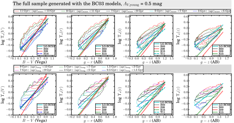
Figure 31.— The four relatively tight optical color–$\log\Upsilon_{\star}$($\lambda$) relations of the sample with $A_{V,{\rm young}}$ = 0 mag, based on the BC03 models. The full sample is grouped by different ranges of $\langle{\rm age}\rangle_{\rm mass}$ and $\langle{\rm age}\rangle_{\lambda,{\rm long}}$, respectively, in the top and bottom panels, as in Figures 4 and 6. Several published linear color–$\log\Upsilon_{\star}$($\lambda$) relations (whenever available for given passbands), as in Figure 3, are overplotted for comparison.

VII.2.1 Bell et al. (2003) Relations

B03 relations are calibrated with a large sample of SDSS galaxies in the local universe. In particular, B03 estimated $\Upsilon_{\star}$($\lambda$) of their galaxies by fitting the SDSS $ugriz$ and 2MASS $JHK$ photometry with dust-free single exponential model SFH libraries, with an [M/H] coverage from $-1.3$ to 0.4. The B03 sample covers color ranges (e.g. 0.2 $\lesssim$ $g$$-$$r$ $\lesssim$ 1.0 mag) blueward of which the optical color–$\log\Upsilon_{\star}$($\lambda$) distributions start strongly deviating (toward lower $\log\Upsilon_{\star}$($\lambda$)) from linear extrapolations at redder colors. Gallazzi & Bell (2009) already showed that, by fixing the starting time of single exponential SFHs to 12 Gyr, the B03 model distributions are skewed toward older average ages and (thus) the resultant color–$\log\Upsilon_{\star}$($\lambda$) distributions are skewed toward larger $\Upsilon_{\star}$($\lambda$) at given color values, as compared to exponential SFHs with smaller starting time. From the comparisons of ($g$$-$$i$)–$\log\Upsilon_{\star}$($i$) and ($g$$-$$z$)–$\log\Upsilon_{\star}$($z$) distributions shown in Figure 31, the B03 relations are largely aligned with the lower-$\log\Upsilon_{\star}$($\lambda$) side of the $\langle{\rm age}\rangle_{\rm mass}$ contour at 11$-$13 Gyr and at the same time the higher-$\log\Upsilon_{\star}$($\lambda$) side of the $\langle{\rm age}\rangle_{\rm mass}$ contour at 5$-$7 Gyr. Therefore, the B03 relations apply to galaxies with 7 Gyr $\lesssim$ $\langle{\rm age}\rangle_{\rm mass}$ $\lesssim$ 11 Gyr.

VII.2.2 Herrmann et al. (2016) Relations

The H16 ($B$$-$$V$)–$\log\Upsilon_{\star}$($V$) relation is calibrated with a representative sample of nearby dwarf irregular galaxies, which cover a ($B$$-$$V$) color range of $\sim$ 0.1 – 0.7 mag. $\log\Upsilon_{\star}$($V$) of the sample galaxies were estimated (Zhang et al. 2012) by fitting the FUV, NUV, $UBV$ and Spitzer 3.6$\mu$m multiband photometry. The monometallic SFH library used by Zhang et al. (2012) covers a [M/H] range from $\sim$ $-1.7$ to $-$0.4, which is appropriate for dwarf irregular galaxies. As discussed in Section IV.4.1, toward the blue end of colors, galaxies with lower [M/H] follow shallower average color–$\log\Upsilon_{\star}$($\lambda$) relations than those with higher [M/H]. Therefore, the slightly shallower H16 relation, as compared to the B03 relation, can be explained by the metallicity coverage of the SFH libraries. Indeed, H16 found that galaxies with lower measured oxygen abundances follow shallower color–$\log\Upsilon_{\star}$($\lambda$) relations.

VII.2.3 Taylor et al. (2011) Relations

The T11 ($g$$-$$i$)–$\log\Upsilon_{\star}$($i$) relation is roughly aligned with the lower-$\log\Upsilon_{\star}$($i$) side of the $\langle{\rm age}\rangle_{\rm mass}$ contour at 7$-$9 Gyr, suggesting a typical $\langle{\rm age}\rangle_{\rm mass}$ $\lesssim$ 7 Gyr. The T11 relation was calibrated by fitting the SDSS $ugriz$ multiband photometry of a large sample of galaxies spanning a redshift range from 0.0 to 0.65 (universe age $\gtrsim$ 7.6 Gyr). The redshift of a galaxy restricts the oldest possible starting time $t$ and thus the $\langle{\rm age}\rangle_{\rm mass}$ of single exponential model SFHs, so the significantly lower $\log\Upsilon_{\star}$($i$) (for given color values) predicted by the T11 relation than that by B03 and the relation followed by the LG dwarf galaxies (LG-BC03) could be attributed to the redshift distribution of the galaxies studied by T11. We note that the nearly linear and particularly tight ($g$$-$$i$)–$\log\Upsilon_{\star}$($i$) distribution followed by the galaxies of T11 is well explained by their relatively young $\langle{\rm age}\rangle_{\rm mass}$ (Section IV.3).

VII.2.4 Zibetti et al. (2009) and Roediger & Courteau (2015) Relations

The Z09 and R15 relations are least-squared regression of the color–$\log\Upsilon_{\star}$($\lambda$) distributions followed by their model SFH libraries. The significantly steeper slopes and smaller intercepts of the Z09 and R15 relations can be explained by their model SFH distributions that are strongly skewed toward younger light-weighted ages at given color values. Indeed, as described in da Cunha et al. (2008), 50% of their model SFHs have experienced a random burst in the past 2 Gyr, with the fractional mass contribution from bursts ranging from 3% to 80%. However, such extremely high mass fraction of recent bursts is actually a very rare phenomenon in nearby galaxies. For instance, Lee et al. (2009b) found that only $\sim$ 6% of nearby dwarf galaxies are currently experiencing massive global bursts with birth-rate parameter $b\geq 2\!-\!3$, and only $\sim$ 23% of the overall star formation in dwarfs occurring in the starburst mode. The burst frequency and strength of more massive galaxies are even lower (e.g. Kauffmann et al. 2003).

In addition, the MAGPHYS package, as used by Z09 and R15, assumes an extinction recipe whereby populations younger than 10 Myr are subject to a steep extinction curve of $A_{\lambda}$ $\propto$ $\lambda^{-1.3}$ while older populations are subject to an extinction curve of $A_{\lambda}$ $\propto$ $\lambda^{-0.7}$. Although da Cunha et al. (2008) claim that adopting a steeper extinction curve solely for the youngest populations has a negligible influence on the emergent integrated SEDs, the steep extinction curve for the youngest populations that may account for an excessively large mass fraction results in a larger spread of $\log\Upsilon_{\star}$($\lambda$) toward the lower right part of the color–$\log\Upsilon_{\star}$($\lambda$) planes (Section IV.5), and thus steepens the average color–$\log\Upsilon_{\star}$($\lambda$) relations.

VII.3. Remarks on the Generality of Our Results

Throughout this work, we have quantified and discussed all of the relevant parameters impacting the determination of stellar masses by using the half max–min ranges, instead of the usually used standard deviations. By doing so, our general conclusions are not limited by the exact shape of the underlying distributions of various physical parameters characterizing the SFHs and metallicity evolution of our samples.

Our samples span a relatively uniform range of $\langle{\rm age}\rangle_{\rm\lambda}$ from $\sim$ 0.5 to 13 Gyr and of $\langle{\rm age}\rangle_{\rm mass}$ from $\sim$ 3 to 13 Gyr (corresponding to an average mass-assembly redshift range from $\sim$ 0.25 to 7). These age ranges cover the average ages measured for local universe galaxies with stellar masses up to 10¹² M_⊙ (Gallazzi et al. 2005). Our finding that the “concentration” of SFHs in time does not significantly affect the color–$\log\Upsilon_{\star}$($\lambda$) relations gives us further confidence that the SFHs of our full sample are adequate for exploring the issue of stellar mass estimation for local universe galaxies in general. In addition, observations suggest that there exists a nearly universal relation between metallicities, SFRs, and stellar masses for galaxies with different stellar masses and redshift (e.g. Hunt et al. 2016). This indicates that the “shape” of metallicity evolution histories is, on average, closely linked to that of the SFHs, while the absolute values of SFRs and stellar masses set the absolute metallicity scales.

Given the above considerations, our full samples are expected to adequately cover the physically plausible range of SFHs and metallicity evolution histories for ordinary galaxies with different masses in the local universe.

VIII. Summary

Taking advantage of the relatively accurate SFHs, the associated metallicity evolution, and age-dependent dust extinction recipe self-consistently determined through resolved CMD modeling of 40 LG dwarf galaxies (Weisz et al. 2014), we derived their expected broadband SEDs and studied their color–$\log\Upsilon_{\star}$($\lambda$) distributions in various broad passbands from the UV to NIR. By expanding the parameter coverages of SFHs in the recent 1 Gyr, average metallicities ([M/H]), and dust extinction of the LG dwarf galaxies, we systematically studied the dependence of color–$\log\Upsilon_{\star}$($\lambda$) distributions on SFHs, mass-weighted ages $\langle{\rm age}\rangle_{\rm mass}$, monochromatic light-weighted ages $\langle{\rm age}\rangle_{\rm\lambda}$ and metallicities $\langle{\rm[M/H]}\rangle_{\rm\lambda}$, metallicity evolution, and dust extinction. In addition, we explored the efficacy of nonparametric broadband SED fitting in recovering the input stellar masses of our expanded sample. The primary results from this work are summarized below.

1. The 40 LG dwarf galaxies follow color–$\log\Upsilon_{\star}$($\lambda$) relations that fall in between the ones calibrated by previous studies. Moreover, the discrepancies between the color–$\log\Upsilon_{\star}$($\lambda$) relations of the LG dwarf galaxies and those from previous studies are generally smaller for color–$\log\Upsilon_{\star}$($\lambda$) relations covering shorter-wavelength baselines, with the ($B$$-$$V$)–$\log\Upsilon_{\star}$($V$) and, to a lesser extent, the ($g$$-$$r$)–$\log\Upsilon_{\star}$($r$) relations being the ones that agree most closely. In addition, we found that the classic BC03 stellar population models give color–$\log\Upsilon_{\star}$$\lambda$) distributions with larger scatter than the FSPS models, but the two models give average color–$\log\Upsilon_{\star}$($\lambda$) relations with consistent slopes and intercepts.

2. The shape of SFHs, as quantified by their concentration in time (i.e. $\log$(t_m,20%/t_m,80%)), does not significantly affect the slopes and intercepts of the color–$\log\Upsilon_{\star}$($\lambda$) relations, except for the most concentrated SFHs (i.e. $\log$(t_m,20%/t_m,80%) $\gtrsim$ 0) which have systematically higher $\Upsilon_{\star}$($\lambda$) at given colors. $\langle{\rm age}\rangle_{\rm\lambda}$ is the physical parameter most closely correlated with $\Upsilon_{\star}$($\lambda$), with its correlation strength peaking at the $J$ and $H$ bands, in analogy to similar correlations between ages and $\Upsilon_{\star}$($\lambda$) of SSPs. Instead of being correlated with $\Upsilon_{\star}$($\lambda$), $\langle{\rm age}\rangle_{\rm mass}$ alone sets the upper and, to a lesser extent, lower limits of $\Upsilon_{\star}$($\lambda$) at given color values. For the SFHs with associated metallicity evolution, $\langle{\rm age}\rangle_{\rm\lambda}$ and $\langle{\rm[M/H]}\rangle_{\rm\lambda}$ together constrain $\log\Upsilon_{\star}$($\lambda$) with uncertainties, as quantified by the half max–min ranges, ranging from $\lesssim$ 0.1 dex for the $J$ and longer-wavelength passbands and up to $\lesssim$ 0.2 dex for the $r$ and shorter-wavelength passbands.

3. SFHs without associated metallicity evolution result in color–$\log\Upsilon_{\star}$($\lambda$) relations that are slightly shallower than but still well consistent with that of SFHs with associated metallicity evolution. Moreover, on the color–$\log\Upsilon_{\star}$($\lambda$) planes, monometallic SFHs with [M/H] fixed to $\langle{\rm[M/H]}\rangle_{\rm\lambda}$ match their multimetallic version of SFHs better than monometallic SFHs with [M/H] fixed to $\langle[\rm M/H]\rangle_{\rm mass}$. The half max–min differences between $\log\Upsilon_{\star}$($\lambda$) resulting from given SFHs with and without metallicity evolution are $\lesssim$ 0.1 dex. Metallicity evolution has a stronger effect on optical–NIR colors ($\lesssim$ 0.3 mag) than optical–optical colors ($\lesssim$ 0.1 mag). By using monometallic SFH models to infer $\log\Upsilon_{\star}$($\lambda$) of real galaxies, one tends to underestimate the uncertainties by $\lesssim$ 0.1 dex.

4. The influence of dust extinction and reddening on color–$\log\Upsilon_{\star}$($\lambda$) distributions depends on the stellar population mixes and the adopted dust extinction curves. In the context of a physically plausible age-dependent dust extinction recipe, dust extinction and reddening barely affect the color–$\log\Upsilon_{\star}$($\lambda$) distributions if the relatively shallow Charlot & Fall (2000) extinction curve ($A_{\lambda}$ $\propto$ $\lambda^{-0.7}$) is adopted, while they can flatten the slopes (by up to 30%) and increase the scatter (by up to 50%) of the resultant optical color–$\log\Upsilon_{\star}$($\lambda$) distributions if the steep average SMC-bar extinction curve is adopted.

5. Regarding the practice of using single NIR passbands as proxies for stellar masses, the $J$ and $H$ bands have smaller max–min ranges of $\log\Upsilon_{\star}$($\lambda$) ($\sim$ 0.7 dex) than either the shorter- or longer-wavelength passbands. However, because $\Upsilon_{\star}$($\lambda$) is strongly correlated with $\langle{\rm age}\rangle_{\rm\lambda}$, especially in the $J$ and $H$ passbands, using luminosities of the $JH$ or other passbands as indicators of stellar masses of galaxies of different types is subject to systematic uncertainties as large as the max–min ranges of $\Upsilon_{\star}$($\lambda$).

6. We searched for the optimal color–$\log\Upsilon_{\star}$($\lambda$) relation for $\Upsilon_{\star}$($\lambda$) estimation in general and find that the $V$ band is the optimal luminance passband for estimating $\Upsilon_{\star}$($\lambda$) based on single colors. In particular, the combinations of $\Upsilon_{\star}$($V$) and optical colors such as $B$$-$$V$, $g$$-$$r$ and $B$$-$$R$ exhibit weaker systematic dependences on SFHs, [M/H], and dust extinction than the combinations involving longer-wavelength luminance passbands. In addition, by partially removing the dependences of optical color–$\log\Upsilon_{\star}$($\lambda$) distributions on [M/H] and dust extinction, optical–NIR colors help to improve the constraints on $\langle{\rm age}\rangle_{\rm\lambda}$ and thus $\Upsilon_{\star}$($\lambda$) in general.

7. With respect to the limitations of recovering stellar masses $\mathcal{M_{\star}}$ of galaxies with relatively low dust extinction ($A_{V}$ $\lesssim$ 0.5 mag) from fitting the integrated broadband SEDs, without any prior assumption on SFHs and metallicity evolution, $\log M_{\star}$ can be constrained with maximum biases of $\lesssim$ 0.3 dex when UV-to-NIR or optical-to-NIR passbands are used in SED fitting, regardless of whether dust extinction is fixed or variable in SED fitting. Optical passbands alone can constrain $\log M_{\star}$ with maximum biases $\lesssim$ 0.4 dex when dust extinction is fixed or $\lesssim$ 0.6 dex when dust extinction is variable in SED fitting. The uncertainties and biases of $\log M_{\star}$ estimation are generally smaller at redder optical colors. Passbands blueward of $g$ are helpful for $\log M_{\star}$ estimation only when NIR passbands are not used in the SED fitting. NIR passbands are more important for improving the $\log M_{\star}$ estimation at higher [M/H], probably due to the generally broader and steeper optical color–$\log\Upsilon_{\star}$($\lambda$) relations. Even with the full FUV-to-NIR SED fitting, $\log M_{\star}$ of galaxies with the oldest (or youngest) $\langle{\rm age}\rangle_{\rm mass}$ tend to be underestimated (or overestimated). Such $\langle{\rm age}\rangle_{\rm mass}$-dependent biases are significantly stronger when NIR passbands are not used for SED fitting. By using purely monometallic SFH models to fit the broadband SEDs of real galaxies, $\log M_{\star}$ has a strong tendency to be underestimated.

Appendix A Linear Least-squares Fitting of the color–$\log\Upsilon_{\star}$($\lambda$) Relations

Following the common practice, we determine the linear least-squares fitting parameters for the optical color–$\log\Upsilon_{\star}$($\lambda$) relations of the 40 LG dwarf galaxies, the default full sample, and the full sample expanded with different $A_{V,{\rm young}}$. For the 40 LG dwarf galaxies, the individual data points are directly used in the linear least-squares fitting, while for the default full sample and the expanded sample, the data points are first binned in color intervals of 0.05 mag, and then the mean of the maximum and minimum $\log\Upsilon_{\star}$($\lambda$) in each color bin is fitted as a function of colors. Note that, for the expanded sample with variable $A_{V,{\rm young}}$, here we only consider “galaxies” with $A_{V,{\rm young}}$ $>$ 0 mag, because no star formation in the present day takes place in a dust-free environment. The fitted slopes $b_{\lambda}$ and intercepts $a_{\lambda}$ are given in Tables 1 and 2 for the samples generated based on the FSPS and BC03 models, respectively.

Table 1Linear least-squares fitting to $\log$$\Upsilon_{\star}$($\lambda$) = $a_{\lambda}$ + ($b_{\lambda}$ $\times$ color) based on FSPS models

Color	$a_{B}$	$b_{B}$	$a_{g}$	$b_{g}$	$a_{V}$	$b_{V}$	$a_{r}$	$b_{r}$	$a_{R}$	$b_{R}$	$a_{i}$	$b_{i}$	$a_{I}$	$b_{I}$	$a_{z}$	$b_{z}$
The 40 LG Dwarf Galaxies
$g$$-$$r$	$-$0.778	1.747	$-$0.684	1.575	$-$0.555	1.322	$-$0.491	1.175	$-$0.481	1.127	$-$0.457	1.012	$-$0.448	0.963	$-$0.447	0.911
$g$$-$$i$	$-$0.802	1.242	$-$0.706	1.120	$-$0.573	0.941	$-$0.508	0.836	$-$0.497	0.802	$-$0.471	0.720	$-$0.461	0.685	$-$0.459	0.647
$g$$-$$z$	$-$0.774	1.030	$-$0.680	0.928	$-$0.550	0.778	$-$0.486	0.690	$-$0.476	0.661	$-$0.451	0.592	$-$0.440	0.561	$-$0.438	0.528
$r$$-$$i$	$-$0.849	4.249	$-$0.749	3.835	$-$0.610	3.224	$-$0.541	2.866	$-$0.529	2.748	$-$0.499	2.466	$-$0.487	2.341	$-$0.483	2.207
$r$$-$$z$	$-$0.729	2.397	$-$0.639	2.157	$-$0.514	1.804	$-$0.453	1.596	$-$0.443	1.527	$-$0.419	1.361	$-$0.408	1.282	$-$0.404	1.196
$B$$-$$V$	$-$0.921	1.632	$-$0.811	1.470	$-$0.661	1.232	$-$0.585	1.094	$-$0.571	1.049	$-$0.537	0.942	$-$0.524	0.896	$-$0.519	0.847
$B$$-$$R$	$-$1.110	1.123	$-$0.982	1.012	$-$0.805	0.849	$-$0.713	0.754	$-$0.693	0.723	$-$0.648	0.650	$-$0.629	0.618	$-$0.618	0.584
$B$$-$$I$	$-$1.254	0.885	$-$1.112	0.797	$-$0.913	0.669	$-$0.809	0.594	$-$0.786	0.569	$-$0.729	0.511	$-$0.706	0.485	$-$0.690	0.457
$V$$-$$R$	$-$1.518	3.581	$-$1.352	3.231	$-$1.117	2.715	$-$0.991	2.414	$-$0.960	2.315	$-$0.888	2.080	$-$0.857	1.978	$-$0.834	1.869
$V$$-$$I$	$-$1.626	1.906	$-$1.448	1.719	$-$1.196	1.442	$-$1.059	1.280	$-$1.025	1.227	$-$0.943	1.100	$-$0.907	1.042	$-$0.877	0.981
$R$$-$$I$	$-$1.710	3.992	$-$1.523	3.596	$-$1.256	3.012	$-$1.111	2.669	$-$1.074	2.556	$-$0.983	2.283	$-$0.941	2.156	$-$0.905	2.017
The Default Full Sample with $A_{V,{\rm young}}=0.5$ mag and an SMC-bar Extinction Curve
$g$$-$$r$	$-$0.629	1.520	$-$0.535	1.355	$-$0.407	1.109	$-$0.345	0.962	$-$0.336	0.913	$-$0.317	0.795	$-$0.313	0.728	$-$0.318	0.647
$g$$-$$i$	$-$0.680	1.085	$-$0.582	0.972	$-$0.448	0.801	$-$0.383	0.698	$-$0.373	0.663	$-$0.351	0.578	$-$0.343	0.529	$-$0.345	0.471
$g$$-$$z$	$-$0.683	0.864	$-$0.584	0.770	$-$0.452	0.632	$-$0.388	0.551	$-$0.378	0.524	$-$0.355	0.457	$-$0.346	0.418	$-$0.347	0.375
$r$$-$$i$	$-$0.714	3.437	$-$0.614	3.072	$-$0.479	2.537	$-$0.414	2.218	$-$0.403	2.110	$-$0.378	1.845	$-$0.367	1.690	$-$0.365	1.511
$r$$-$$z$	$-$0.680	1.841	$-$0.587	1.651	$-$0.458	1.363	$-$0.396	1.189	$-$0.386	1.131	$-$0.364	0.987	$-$0.355	0.904	$-$0.354	0.807
$B$$-$$V$	$-$0.747	1.440	$-$0.638	1.281	$-$0.490	1.046	$-$0.417	0.906	$-$0.404	0.860	$-$0.375	0.747	$-$0.364	0.682	$-$0.360	0.603
$B$$-$$R$	$-$0.937	0.997	$-$0.811	0.890	$-$0.634	0.730	$-$0.544	0.634	$-$0.525	0.602	$-$0.481	0.524	$-$0.461	0.479	$-$0.449	0.426
$B$$-$$I$	$-$1.072	0.765	$-$0.931	0.684	$-$0.735	0.563	$-$0.632	0.489	$-$0.609	0.464	$-$0.554	0.403	$-$0.527	0.368	$-$0.506	0.327
$V$$-$$R$	$-$1.267	3.021	$-$1.108	2.702	$-$0.885	2.232	$-$0.766	1.948	$-$0.737	1.853	$-$0.670	1.620	$-$0.636	1.486	$-$0.606	1.328
$V$$-$$I$	$-$1.393	1.587	$-$1.219	1.416	$-$0.974	1.164	$-$0.844	1.015	$-$0.813	0.966	$-$0.736	0.845	$-$0.698	0.777	$-$0.664	0.698
$R$$-$$I$	$-$1.359	2.955	$-$1.191	2.641	$-$0.950	2.163	$-$0.819	1.873	$-$0.787	1.775	$-$0.708	1.537	$-$0.667	1.399	$-$0.630	1.239
The Full Sample with Variable $A_{V,{\rm young}}$ and an SMC-bar Extinction Curve
$g$$-$$r$	$-$0.635	1.469	$-$0.539	1.311	$-$0.408	1.064	$-$0.346	0.912	$-$0.337	0.860	$-$0.315	0.727	$-$0.308	0.647	$-$0.309	0.542
$g$$-$$i$	$-$0.661	0.995	$-$0.564	0.891	$-$0.431	0.726	$-$0.366	0.624	$-$0.356	0.588	$-$0.330	0.494	$-$0.322	0.438	$-$0.320	0.366
$g$$-$$z$	$-$0.621	0.709	$-$0.529	0.631	$-$0.402	0.509	$-$0.340	0.433	$-$0.330	0.406	$-$0.305	0.335	$-$0.295	0.292	$-$0.291	0.236
$r$$-$$i$	$-$0.631	2.637	$-$0.542	2.363	$-$0.416	1.918	$-$0.354	1.636	$-$0.344	1.533	$-$0.318	1.263	$-$0.307	1.098	$-$0.299	0.868
$r$$-$$z$	$-$0.554	1.254	$-$0.474	1.126	$-$0.360	0.912	$-$0.306	0.776	$-$0.298	0.726	$-$0.277	0.593	$-$0.268	0.509	$-$0.262	0.389
$B$$-$$V$	$-$0.736	1.407	$-$0.627	1.250	$-$0.479	1.013	$-$0.407	0.871	$-$0.394	0.823	$-$0.366	0.702	$-$0.355	0.630	$-$0.350	0.535
$B$$-$$R$	$-$0.926	0.971	$-$0.800	0.866	$-$0.621	0.705	$-$0.530	0.607	$-$0.511	0.574	$-$0.465	0.489	$-$0.444	0.439	$-$0.427	0.374
$B$$-$$I$	$-$1.036	0.717	$-$0.900	0.643	$-$0.706	0.525	$-$0.604	0.452	$-$0.580	0.426	$-$0.520	0.360	$-$0.491	0.320	$-$0.462	0.269
$V$$-$$R$	$-$1.202	2.755	$-$1.049	2.463	$-$0.825	2.002	$-$0.704	1.716	$-$0.673	1.614	$-$0.596	1.354	$-$0.558	1.198	$-$0.513	0.991
$V$$-$$I$	$-$1.210	1.302	$-$1.053	1.158	$-$0.825	0.932	$-$0.701	0.794	$-$0.669	0.744	$-$0.587	0.616	$-$0.543	0.540	$-$0.495	0.441
$R$$-$$I$	$-$1.130	2.288	$-$0.989	2.047	$-$0.777	1.653	$-$0.661	1.408	$-$0.631	1.319	$-$0.555	1.089	$-$0.513	0.949	$-$0.465	0.760

Note. — Linear least-squares fitting to optical color–$\log\Upsilon_{\star}$($\lambda$) distributions of our samples generated based on the FSPS models and the Chabrier (2003) IMF. The monochromatic mass-to-light ratios $\Upsilon_{\star}$($\lambda$) are in solar units. The SDSS $griz$ filters are in the AB magnitude system. The Johnson–Cousins $BVRI$ filters are in the Vega magnitude system.

Table 2Linear least-squares fitting to $\log$$\Upsilon_{\star}$($\lambda$) = $a_{\lambda}$ + ($b_{\lambda}$ $\times$ color) based on BC03 models

Color	$a_{B}$	$b_{B}$	$a_{g}$	$b_{g}$	$a_{V}$	$b_{V}$	$a_{r}$	$b_{r}$	$a_{R}$	$b_{R}$	$a_{i}$	$b_{i}$	$a_{I}$	$b_{I}$	$a_{z}$	$b_{z}$
The 40 LG Dwarf Galaxies
$g$$-$$r$	$-$0.842	1.786	$-$0.745	1.616	$-$0.617	1.367	$-$0.552	1.216	$-$0.540	1.164	$-$0.511	1.038	$-$0.504	0.988	$-$0.501	0.937
$g$$-$$i$	$-$0.837	1.227	$-$0.739	1.109	$-$0.612	0.937	$-$0.547	0.833	$-$0.534	0.797	$-$0.505	0.709	$-$0.497	0.674	$-$0.494	0.638
$g$$-$$z$	$-$0.808	1.020	$-$0.712	0.920	$-$0.587	0.776	$-$0.523	0.687	$-$0.511	0.657	$-$0.482	0.582	$-$0.474	0.552	$-$0.470	0.520
$r$$-$$i$	$-$0.808	3.844	$-$0.711	3.467	$-$0.586	2.924	$-$0.523	2.592	$-$0.511	2.476	$-$0.481	2.192	$-$0.474	2.076	$-$0.469	1.956
$r$$-$$z$	$-$0.725	2.270	$-$0.634	2.039	$-$0.517	1.709	$-$0.459	1.507	$-$0.448	1.435	$-$0.422	1.260	$-$0.415	1.186	$-$0.410	1.107
$B$$-$$V$	$-$0.981	1.689	$-$0.869	1.526	$-$0.721	1.289	$-$0.643	1.145	$-$0.627	1.095	$-$0.587	0.975	$-$0.576	0.927	$-$0.568	0.878
$B$$-$$R$	$-$1.160	1.140	$-$1.031	1.030	$-$0.858	0.871	$-$0.766	0.773	$-$0.743	0.740	$-$0.691	0.659	$-$0.675	0.626	$-$0.662	0.593
$B$$-$$I$	$-$1.288	0.879	$-$1.146	0.794	$-$0.954	0.670	$-$0.850	0.595	$-$0.823	0.569	$-$0.761	0.505	$-$0.740	0.479	$-$0.722	0.453
$V$$-$$R$	$-$1.528	3.502	$-$1.365	3.166	$-$1.141	2.678	$-$1.018	2.381	$-$0.985	2.278	$-$0.906	2.029	$-$0.880	1.929	$-$0.856	1.828
$V$$-$$I$	$-$1.610	1.822	$-$1.435	1.643	$-$1.197	1.386	$-$1.065	1.229	$-$1.028	1.174	$-$0.940	1.040	$-$0.909	0.986	$-$0.880	0.929
$R$$-$$I$	$-$1.662	3.716	$-$1.478	3.343	$-$1.228	2.809	$-$1.088	2.483	$-$1.048	2.368	$-$0.952	2.085	$-$0.916	1.968	$-$0.882	1.845
The Default Full Sample with $A_{V,{\rm young}}=0.5$ mag and an SMC-bar Extinction Curve
$g$$-$$r$	$-$0.690	1.566	$-$0.601	1.410	$-$0.475	1.169	$-$0.411	1.020	$-$0.402	0.969	$-$0.382	0.848	$-$0.380	0.793	$-$0.381	0.721
$g$$-$$i$	$-$0.738	1.128	$-$0.646	1.021	$-$0.517	0.855	$-$0.451	0.751	$-$0.440	0.716	$-$0.416	0.630	$-$0.414	0.590	$-$0.413	0.538
$g$$-$$z$	$-$0.742	0.914	$-$0.651	0.829	$-$0.523	0.696	$-$0.455	0.611	$-$0.444	0.582	$-$0.420	0.511	$-$0.416	0.478	$-$0.414	0.435
$r$$-$$i$	$-$0.770	3.381	$-$0.674	3.071	$-$0.546	2.607	$-$0.480	2.314	$-$0.469	2.206	$-$0.446	1.946	$-$0.442	1.819	$-$0.439	1.650
$r$$-$$z$	$-$0.707	1.722	$-$0.621	1.570	$-$0.503	1.341	$-$0.442	1.192	$-$0.432	1.133	$-$0.409	0.987	$-$0.405	0.913	$-$0.401	0.811
$B$$-$$V$	$-$0.842	1.527	$-$0.735	1.371	$-$0.585	1.134	$-$0.510	0.992	$-$0.498	0.946	$-$0.468	0.831	$-$0.462	0.779	$-$0.457	0.709
$B$$-$$R$	$-$1.030	1.057	$-$0.906	0.951	$-$0.731	0.793	$-$0.638	0.696	$-$0.619	0.663	$-$0.576	0.584	$-$0.564	0.548	$-$0.550	0.500
$B$$-$$I$	$-$1.185	0.821	$-$1.050	0.742	$-$0.854	0.621	$-$0.747	0.545	$-$0.721	0.519	$-$0.663	0.455	$-$0.643	0.426	$-$0.621	0.388
$V$$-$$R$	$-$1.340	3.131	$-$1.185	2.822	$-$0.965	2.357	$-$0.847	2.075	$-$0.819	1.980	$-$0.756	1.752	$-$0.736	1.648	$-$0.711	1.509
$V$$-$$I$	$-$1.463	1.621	$-$1.302	1.467	$-$1.068	1.231	$-$0.936	1.082	$-$0.901	1.029	$-$0.821	0.902	$-$0.790	0.842	$-$0.753	0.763
$R$$-$$I$	$-$1.415	2.888	$-$1.266	2.629	$-$1.052	2.240	$-$0.929	1.988	$-$0.894	1.888	$-$0.810	1.639	$-$0.774	1.513	$-$0.728	1.339
The Full Sample with Variable $A_{V,{\rm young}}$ and an SMC-bar Extinction Curve
$g$$-$$r$	$-$0.701	1.550	$-$0.608	1.394	$-$0.479	1.148	$-$0.417	0.998	$-$0.410	0.948	$-$0.390	0.818	$-$0.389	0.756	$-$0.389	0.667
$g$$-$$i$	$-$0.732	1.049	$-$0.639	0.948	$-$0.509	0.788	$-$0.444	0.685	$-$0.432	0.647	$-$0.406	0.552	$-$0.401	0.506	$-$0.396	0.439
$g$$-$$z$	$-$0.695	0.764	$-$0.606	0.691	$-$0.484	0.573	$-$0.421	0.498	$-$0.410	0.468	$-$0.383	0.393	$-$0.376	0.354	$-$0.368	0.296
$r$$-$$i$	$-$0.664	2.540	$-$0.575	2.298	$-$0.456	1.910	$-$0.397	1.661	$-$0.386	1.555	$-$0.360	1.285	$-$0.353	1.141	$-$0.343	0.924
$r$$-$$z$	$-$0.597	1.187	$-$0.518	1.084	$-$0.409	0.908	$-$0.357	0.794	$-$0.347	0.741	$-$0.326	0.602	$-$0.319	0.524	$-$0.309	0.403
$B$$-$$V$	$-$0.811	1.473	$-$0.702	1.317	$-$0.552	1.078	$-$0.478	0.935	$-$0.468	0.889	$-$0.440	0.770	$-$0.435	0.713	$-$0.432	0.634
$B$$-$$R$	$-$1.016	1.030	$-$0.890	0.926	$-$0.712	0.764	$-$0.621	0.667	$-$0.604	0.635	$-$0.559	0.551	$-$0.546	0.510	$-$0.529	0.453
$B$$-$$I$	$-$1.147	0.773	$-$1.015	0.699	$-$0.821	0.581	$-$0.715	0.506	$-$0.688	0.479	$-$0.625	0.409	$-$0.601	0.375	$-$0.570	0.326
$V$$-$$R$	$-$1.259	2.820	$-$1.118	2.554	$-$0.906	2.115	$-$0.787	1.834	$-$0.756	1.729	$-$0.679	1.467	$-$0.650	1.338	$-$0.610	1.153
$V$$-$$I$	$-$1.285	1.340	$-$1.138	1.209	$-$0.926	1.003	$-$0.805	0.871	$-$0.771	0.818	$-$0.685	0.684	$-$0.646	0.614	$-$0.591	0.511
$R$$-$$I$	$-$1.147	2.166	$-$1.019	1.974	$-$0.828	1.659	$-$0.722	1.445	$-$0.690	1.352	$-$0.609	1.112	$-$0.572	0.983	$-$0.516	0.789

Note. — Same as Table 1, with the exception that here the optical color–$\log\Upsilon_{\star}$($\lambda$) distributions of our samples are generated based on the BC03 models.

References

- Alongi et al. (1993) Alongi, M., Bertelli, G., Bressan, A., et al., 1993, A&AS, 97, 851
- Acquaviva et al. (2011) Acquaviva, V., Gawiser, E., Guaita, L., 2011, ApJ, 737, 47
- Arnouts & IIbert (2011) Arnouts, S., Ilbert, O., 2011, LePHARE: Photometric Analysis for Redshift Estimate, astrophysics Source Code Library, ascl: 1108.009
- Baldwin et al. (2017) Baldwin, C. M., McDermid, R. M., Kuntschner, H., Maraston, C., Conroy, C., arXiv:1709.09300
- Bressan et al. (1993) Bressan, A., Fagotto, F., Bertelli, G., Chiosi, C., 1993, A&AS, 100, 647
- Brinchmann & Ellis (2000) Brinchmann, J., Ellis, R. S., 2000, ApJL, 536, 77
- Bershady et al. (2000) Bershady, M.A., Jangren, J.A., Conselice, C.J. 2000, AJ, 119, 2645
- Bolzonella et al. (2000) Bolzonella, M., Miralles, J.M., Pelló, R., 2000, A&A, 363, 476
- Bolzonella et al. (2010) Bolzonella, M., Kovac, K., Pozzetti, L., Zucca, E., Cucciati, O., et al., 2010, A&A, 524, 76
- Bell & de Jong (2001) Bell, E. F. & de Jong, R. S. 2001, ApJ, 550, 212
- Bell et al. (2003) Bell, E. F., McIntosh, D. H., Katz, N., Weinberg, M. D., 2003, ApJS, 149, 289
- Bruzual & Charlot (2003) Bruzual, G., Charlot, S., 2003, MNRAS, 344, 1000 (BC03)
- Borch et al. (2006) Borch, A., Meisenheimer, K., Bell, E.F. et al., 2006, A&A, 453, 869
- Blanton & Roweis (2007) Blanton, M. R., Roweis, S. 2007, AJ, 133, 734
- Brammer et al. (2008) Brammer, G.B., van Dokkum, P.G., Coppi, P., 2008, ApJ, 686, 1503
- Bendo et al. (2015) Bendo, G.J., Baes, M., Bianchi, S., et al. 2015, MNRAS, 448, 135
- Battisti et al. (2016) Battisti, A.J., Calzetti, D., Chary, R.-R., 2016, ApJ, 818, 13
- Charlot & Fall (2000) Charlot, S., Fall, S.M., 2000, ApJ, 539, 718
- Chabrier (2003) Chabrier, G. 2003, PASP, 115, 763
- Cid Fernandes et al. (2005) Cid Fernandes, R., Mateus, A., Sodre, L., et al. 2005, MNRAS, 358, 363
- Conroy et al. (2009) Conroy, C., Gunn, J. E., White, M., 2009, ApJ, 699, 486
- Conroy & Gunn (2010) Conroy, C., Gunn, J. E. 2010, ApJ, 712, 833
- Conroy (2013) Conroy, C., 2013, ARA&A, 51, 393
- Cole et al. (2007) Cole, A. A., Skillman, E. D., Tolstoy, E., et al. 2007, ApJ, 659, 17
- Cole et al. (2014) Cole, A. A., Weisz, D. R., Dolphin, A. E., et al. 2014, ApJ, 795, 54
- Chen et al. (2012) Chen, Y. M., Kauffmann, G., Tremonti, C., et al., 2012, MNRAS, 421, 314
- Chevallard et al. (2013) Chevallard, J., Charlot, S., Wandelt, B., Wild, V., 2013, MNRAS, 432, 2061
- Calzetti et al. (1994) Calzetti, D., Kinney, A.L., Storchi-Bergmann, T., 1994, ApJ, 429, 582
- Chevallard & Charlot (2016) Chevallard, J., Charlot, S., 2016, MNRAS, 462, 1415
- Cappellari (2017) Cappellari, M. 2017, MNRAS, 466, 798
- Dolphin et al. (2003) Dolphin, A. E., Saha, A., Skillman, E. D., Dohm-Palmer, R. C. 2003, AJ, 2003, 126, 187
- Dabringhausen et al. (2008) Dabringhausen, J., Hilker, M., & Kroupa, P. 2008, MNRAS, 386, 864
- da Cunha et al. (2008) da Cunha, E., Charlot, S., & Elbaz, D. 2008, MNRAS, 388, 1595
- Eldridge & Stanway (2009) Eldridge, J. J., Stanway, E. R., 2009, MNRAS, 400, 1019
- El-Badry et al. (2017) El-Badry, K., Weisz, D. R., Quataert, E., 2017, MNRAS, 468, 319
- Fagotto et al. (1994a) Fagotto, F., Bressan, A., Bertelli, G., Chiosi, C., 1994a, A&AS, 104, 365
- Fagotto et al. (1994b) Fagotto, F., Bressan, A., Bertelli, G., Chiosi, C., 1994b, A&AS, 105, 29
- Fioc & Rocca-Volmerange (1997) Fioc, M., Rocca-Volmerange, B., 1997, A&A, 326, 950
- Ford et al. (1998) Ford, H. C., Bartko, F., Bely, P. Y., et al. 1998, Proc. SPIE, 3356, 234
- Flaugher (2005) Flaugher, B., 2005, International Journal of Modern Physics A. 20, 3121
- Geha et al. (2013) Geha, M., Brown, T. M., Tumlinson, J., et al. 2013, ApJ, 771, 29
- Girardi et al. (1996) Girardi, L., Bressan, A., Chiosi, C., et al., 1996, A&AS, 117, 113
- Girardi et al. (2000) Girardi, L., Bressan, A., Bertelli, G., et al., 2000, A&AS, 141, 371
- Gordon et al. (2003) Gordon, K.D., Clayton, G.C., Misselt, K.A., et al. 2003, ApJ, 594, 279
- Gallazzi et al. (2005) Gallazzi, A., Charlot, S., Brinchmann, J., et al., 2005, MNRAS, 362, 41
- Gallazzi & Bell (2009) Gallazzi, A., Bell, E.F., 2009, ApJS, 185, 253
- Holtzman et al. (1995) Holtzman, J. A., Burrows, C. J., Casertano, S., et al. 1995, PASP, 107, 1065
- Hunter & Hoffman (1999) Hunter, D. A., Hoffman, L., 1999, AJ, 117, 2789
- Hidalgo et al. (2011) Hidalgo, S. L., Aparicio, A., Skillman, E., et al. 2011, ApJ, 730, 14
- Han & Han (2014) Han, Y., Han, Z., 2014, ApJS, 215, 2
- Hayward & Smith (2015) Hayward, C.C., Smith, D.J.B. 2015, MNRAS, 446, 1512
- Heavens et al. (2000) Heavens, A. F., Jimenez, R., Lahav, O., 2000, MNRAS, 317, 965
- Herrmann et al. (2016) Herrmann, K. A., Hunter, D. A., Zhang, H.-X., Elmegreen, B. G. 2016, AJ, 152, 177
- Hunt et al. (2016) Hunt, L., Dayal, P., Magrini, L., Ferrara, A., et al. 2016, MNRAS, 463, 2002
- Ivezic et al. (2008) Ivezic, Z., Tyson, J. A., Abel, B., et al. 2008, arXiv:0805.2366
- Into & Portinari (2013) Into, T., Portinari, L. 2013, MNRAS, 430, 2715
- Iyer & Gawiser (2017) Iyer, K., Gawiser, E., 2017, ApJ, 838, 127
- Jarrett et al. (2000) Jarrett, T.H., Chester, T., Cutri, R. et al., 2000, AJ, 119, 2498
- Johnson et al. (2013a) Johnson, B. D., Weisz, D. R., Dalcanton, J. J. et al. 2013a, ApJ, 772, 8
- Johnson et al. (2013b) Johnson, S.P., Wilson, G.W., Tang, Y., Scott, K.S., 2013b, MNRAS, 436, 2535
- Kroupa (2001) Kroupa, P. 2001, MNRAS, 322, 231
- Kauffmann et al. (2003) Kauffmann, G., Heckman, T.M., White, S.D.M. et al. 2003, MNRAS, 341, 33
- Kannappan & Gawiser (2007) Kannappan, S. J., Gawiser, E., 2007, ApJ, 657, 5
- Kotulla et al. (2009) Kotulla, R., Fritze, U., Weilbacher, P., Anders, P., 2009, MNRAS, 396, 462
- Karachentsev et al. (2013) Karachentsev, I. D., Makarov, D. I., Kaisina,, E. I., 2013, AJ, 145, 101
- Lawson & Hanson (1974) Lawson, C. L., & Hanson, R. J., Solving Least Squares Problems, First Edition, Prentice-Hall, Englewood Cliffs, N. J., 1974
- Leitherer et al. (1999) Leitherer, C., Schaerer, D., Goldader, J. D., et al. 1999, ApJS, 123, 3
- Lee et al. (2009a) Lee, S.-K., Idzi, R., Ferguson, H.C. et al., 2009a, ApJS, 184, 100
- Lee et al. (2009b) Lee, J.C., Kennicutt, R.C. Jr., Funes, J.G. et al. 2009b, ApJ, 692, 1305
- Leja et al. (2017) Leja, J., Johnson, B.D., Conroy, C. et al., 2017, ApJ, 837, 170
- Lo Faro et al. (2017) Lo Faro, B., Buat, V., Roehlly, Y. et al., 2017, MNRAS, 472, 1472
- Martin et al. (2005) Martin, D. C., Fanson, J., Schiminovich, D. et al., 2005, ApJ, 619, 1
- Marigo & Girardi (2007) Marigo, P., Girardi, L., 2007, A&A, 469, 239
- Marigo et al. (2008) Marigo, P., Girardi, L., Bressan, A., et al. 2008, A&A, 482, 883
- Madau & Dickinson (2014) Madau, P., Dickinson, M., 2014, ARA&A, 52, 415
- Mobasher et al. (2015) Mobasher, B., Dahlen, T., Ferguson, H.C. et al., 2015, ApJ, 808, 101
- Maraston (2005) Maraston, C., 2005, MNRAS, 362, 799
- Maraston et al. (2006) Maraston, C., Daddi, E., Renzini, A., et al. 2006, ApJ, 652, 85
- Maraston et al. (2013) Maraston, C., Pforr, J., Henriques, B.M. et al., 2013, MNRAS, 435, 2764
- McQuinn et al. (2010) McQuinn, K. B. W., Skillman, E. D., Cannon, J. M., et al. 2010, ApJ, 724, 49
- Moultaka & Pelat (2000) Moultaka, J., Pelat, D. 2000, MNRAS, 314, 409
- Moustakas et al. (2013) Moustakas, J., Coil, A. L., Aird, J., et al., 2013, ApJ, 767, 50
- Mitchell et al. (2013) Mitchell, P.D., Lacey, C.G., Baugh, C.M., Cole, S. 2013, MNRAS, 435, 87
- Meinshausen (2013) Meinshausen, N. 2013, Electronic Journal of Statistics, 7, 1607
- McGaugh & Schombert (2014) McGaugh, S. S., Schombert, J. M. 2014, AJ, 148, 77
- Michałowski et al. (2014) Michałowski, M., Hayward, C.C., Dunlop, J.S. et al., 2014, A&A, 571, 75
- McConnell et al. (2016) McConnell, N. J., Lu, J. R., Mann, A. W., 2016, ApJ, 821, 39
- Naab & Ostriker (2017) Naab, T., Ostriker, J.P. 2017, ARA&A, 55, 59
- Noll et al. (2009) Noll, S., Burgarella, D., Giovannoli, E., et al. 2009, A&A, 507, 1793
- Ocvirk et al. (2006a) Ocvirk, P., Pichon, C., Lancon, A., Thiebaut, E. 2006a, MNRAS, 365, 74
- Ocvirk et al. (2006b) Ocvirk, P., Pichon, C., Lancon, A., et al. 2006b, MNRAS, 365, 46
- Offner (2016) Offner, S. S. R., 2016, IAUS, 315, 73
- Press et al. (1992) Press, W. H., Teukolsky, S. A., Vetterling, W. T., Flannery, B. P., 1992, Numerical Recipes in FORTRAN. The Art of Scientific Computing. Cambridge Univ. Press, Cambridge
- Papovich et al. (2001) Papovich, C., Dickinson, M., Ferguson, H.C., 2001, ApJ, 559, 620
- Panter et al. (2007) Panter, B., Jimenez, R., Heavens, A. F., Charlot, S., 2007, MNRAS, 378, 1550
- Portinari et al. (2004) Portinari, L., Sommer-Larsen, J., Tantalo, R. 2004, MNRAS, 347, 691
- Pietrinferni et al. (2004) Pietrinferni, A., Cassisi, S., Salaris, M., Castelli, F., 2004, ApJ, 612, 168
- Pozzetti et al. (2007) Pozzetti, L., Bolzonella, M., Lamareille, F. et al., 2007, A&A, 474, 443
- Popescu et al. (2011) Popescu, C.C., Tuffs, R.J., Dopita, M.A., et al. 2011, A&A, 527, 109
- Powalka et al. (2017) Powalka, M., Lançon, A., Puzia, T. H., et al. 2017, ApJ, 844, 104
- Pacifici et al. (2012) Pacifici, C., Charlot, S., Blaizot, J., Brinchmann, J. 2012, MNRAS, 421, 2002
- Pforr et al. (2012) Pforr, J., Maraston, C., Tonini, C., 2012, MNRAS, 422, 3285
- Pforr et al. (2013) Pforr, J., Maraston, C., Tonini, C., 2013, MNRAS, 435, 1389
- Peacock et al. (2014) Peacock, M. B., Zepf, S. E., Maccarone, T. J., et al. 2014, ApJ, 784, 162
- Rich et al. (1997) Rich, R. M., Sosin, C., Djorgovski, S., et al. 1997, ApJ, 484, L25
- Reddy et al. (2015) Reddy, N.A., Kriek, M., Shapley, A. et al., 2015, ApJ, 806, 259
- Roediger & Courteau (2015) Roediger, J. C., Courteau, S., 2015, MNRAS, 452, 3209
- Scalo (1986) Scalo, J. M. 1986, Fundam. Cosm. Phys. 11, 1
- Sawicki & Yee (1998) Sawicki, M., Yee, H.K.C., 1998, AJ, 115, 1329
- Silva et al. (1998) Silva, L, Granato, G. L., Bressan, A., Danese, L. 1998, ApJ, 509, 103
- Schaye et al. (2015) Schaye, J., Crain, R. A., Bower, R. G., et al., 2015, MNRAS, 446, 521
- Smith et al. (2015) Smith, R. J., Lucey, J. R., Conroy, C. 2015, MNRAS, 449, 3441
- Salim et al. (2016) Salim, S., Lee, J. C., Janowiecki, S., et al. 2016, ApJS, 227, 2
- Tojeiro et al. (2007) Tojeiro, R., Heavens, A. F., Jimenez, R., et al. 2007, MNRAS, 381, 1252
- Tolstoy et al. (2009) Tolstoy, E., Hill, V., Tosi, M. et al., 2009, ARAA, 47, 371
- Taylor et al. (2011) Taylor, E. N., Hopkins, A. M., Baldry, I. K., et al. 2011, MNRAS, 418, 1587
- Vogelsberger et al. (2014) Vogelsberger, M., Genel, S.; Springel, V., et al., 2014, Nature, 509, 177
- van den Bergh (1999) van den Bergh, S., 1999, A&ARv, 9, 273
- van Dokkum & Conroy (2012) van Dokkum, P. G., Conroy, C., 2012, ApJ, 760, 70
- Worthey (1994) Worthey, G., 1994, ApJS, 95, 107
- Worthey et al. (1994) Worthey, G., Faber, S.M., Gonzalez, J.J., Burstein, D. 1994, ApJS, 94, 687
- Wyse et al. (2002) Wyse, R. F. G., Gilmore, G., Houdashelt, M. L., et al. 2002, NewA, 7, 395
- Wuyts et al. (2009) Wuyts, S., Franx, M., Cox, T.J. et al., 2009, ApJ, 696, 348
- Wuyts et al. (2011) Wuyts, S., Schreiber, N. M. F., Lutz, D., et al. 2011, ApJ, 738, 106
- Wright et al. (2010) Wright, E.L., Eisenhardt, P. R. M., Mainzer, A. K., et al., 2010, AJ, 140, 1868
- Weisz et al. (2011) Weisz, D. R., Dalcanton, J. J., Williams, B. F. et al., 2011, ApJ, 739, 5
- Weisz et al. (2014) Weisz, D. R., Dolphin, A. E., Skillman, E. D. et al., 2014, ApJ, 789, 148 (W14)
- Wild et al. (2011) Wild, V., Charlot, S., Brinchmann, J. et al., 2011, MNRAS, 417, 1760
- Walcher et al. (2011) Walcher, J., Groves, B., Budavári, T., et al. 2011, Ap&SS, 331, 1
- Xilouris et al. (1999) Xilouris, E. M., Byun, Y.I., Kylafis, N. D., et al. 1999, A&A, 344, 868
- York et al. (2000) York, D. G., Adelman, J., Anderson, J. E. et al., 2000, AJ, 120, 1579
- Yoachim & Dalcanton (2006) Yoachim, P., Dalcanton, J. J. 2006, AJ, 131, 226
- Zibetti et al. (2009) Zibetti, S., Charlot, S., Rix, H.-W., 2009, MNRAS, 400, 1181
- Zhao et al. (2011) Zhao, Y., Gu, Q., Gao, Y., 2011, AJ, 141, 68
- Zhang et al. (2012) Zhang, H.-X., Hunter, D. A., Elmegreen, B. G., Gao, Y., Schruba, A., 2012, AJ, 143, 47