Isochoric, isobaric and ultrafast conductivities of
aluminum, lithium and carbon in the warm dense matter regime

Abstract

We study the conductivities $\sigma$ of (i) the equilibrium isochoric state ($\sigma_{\rm is}$), (ii) the equilibrium isobaric state ($\sigma_{\rm ib}$), and also the (iii) non-equilibrium ultrafast matter (UFM) state ($\sigma_{\rm uf}$) with the ion temperature $T_{i}$ less than the the electron temperature $T_{e}$. Aluminum, lithium and carbon are considered, being increasingly complex warm dense matter (WDM) systems, with carbon having transient covalent bonds. First-principles calculations, i.e., neutral-pseudoatom (NPA) calculations and density-functional theory (DFT) with molecular-dynamics (MD) simulations, are compared where possible with experimental data to characterize $\sigma_{\rm ic},\sigma_{\rm ib}$ and $\sigma_{\rm uf}$. The NPA $\sigma_{\rm ib}$ are closest to the available experimental data when compared to results from DFT+MD, where simulations of about 64-125 atoms are typically used. The published conductivities for Li are reviewed and the value at a temperature of 4.5 eV is examined using supporting X-ray Thomson scattering calculations. A physical picture of the variations of $\sigma$ with temperature and density applicable to these materials is given. The insensitivity of $\sigma$ to $T_{e}$ below 10 eV for carbon, compared to Al and Li, is clarified.

I Introduction

Short-pulsed lasers as well as shock-wave techniques can probe matter in hitherto experimentally inaccessible regimes of great interest. These provide information needed for understanding normal matter and unusual states of matter, in equilibrium or in transient conditions Ng2011 ; Milchberg88 . Similar ‘hot-carrier’ processes occur in semiconductor nanostructures DharmaHot93 ; Vaziri2013 . Such warm dense matter (WDM) systems include not only equilibrium systems where the ion temperature $T_{i}$ and the electron temperature $T_{e}$ are equal, but also systems where $T_{i}\neq T_{e}$, or highly non-equilibrium systems where the notion of temperature is inapplicable Medvedev . While the prediction of a quasi equation of state (quasi EOS) and related static properties for two-temperature (2$T$) systems HarbPhon17 is satisfactory, the conductivity calculations using standard codes, even for sodium at the melting point, require massive quantum simulations with as much as $\sim$1500 atoms and over 56 $k$-points (according to Ref. Pozzo11 ), whereas even theories of the 1980s evaluated the sodium conductivities successfully via a momentum relaxation-time ($\tau_{\rm mr}$) approach Sinha89 , which is also used in Drude fits to the Kubo-Greenwood (KG) formula used with density-functional theory (DFT) and molecular dynamics (MD) methods. The KG-formula and its scope are discussed further in the Appendix.

The static electrical conductivities of WDM equilibrium systems (i.e., $T_{i}=T_{e}$), as well as 2$T$ quasiequilibrium systems, are the object of the present study. We distinguish the isobaric equilibrium conductivity $\sigma_{\rm ib}$ and the isochoric equilibrium conductivity $\sigma_{\rm ic}$ from the ultrafast matter (UFM) quasiequilibrium (isochoric) conductivity $\sigma_{\rm uf}$. The 2$T$ WDM states exist only for times shorter than the electron-ion equilibration time $\tau_{\rm ei}$ and may be accessed using femtosecond probes.

We consider three systems of increasing complexity above the melting point: (a) a ‘simple’ system, viz., WDM-aluminum at density $\rho$ =2.7 g/cm³; (b) WDM-lithium at 0.542 g/cm³; and (c) WDM-carbon (2.0-3.7 g/cm³) including the low-$T$ covalent-bonding regime. As experimental data are available for the isobaric evolution of Al and Li starting from their nominal normal densities and down to lower densities of the expanded fluid, we calculate $\sigma_{\rm ib}$ for Al and Li. The ultrafast conductivity $\sigma_{\rm uf}$ is calculated for all three materials, as $\sigma_{\rm is}$ is conveniently accessible via short-pulse laser experiments.

The electrons in WDM-Li are known to be non-local with complex interaction effects. For instance, clustering effects may appear bonev2008 as the density is increased. WDM-carbon is a complex liquid with transient covalent bonding where the C-C bond energy $E_{cc}$ may reach $\sim 8$ eV in dilute gases. The three conductivities $\sigma_{\rm ic}$, $\sigma_{\rm ib}$, and $\sigma_{\rm uf}$ for Al, Li and C, are calculated via two first-principles methods where, however, both finally use a ‘mean-free path’ model to estimate the conductivity. The two methods are: (i) the neutral pseudoatom (NPA) method as formulated by Perrot and Dharma-wardana  HarbPhon17 ; CPP ; eos95 ; Pe-Be together with the Ziman formula, and (ii) the DFT+MD and KG approach as available in codes such as VASP and ABINIT codes , enabling us to assess the extent of the agreement among these theoretical methods and the available experiments. The liquid-metal experimental data are still the most accurate data on WDM systems available; they are used where possible to compare with calculations.

Accurate experimental data for the isobaric liquid state of Al IJTher83 ; Gathers86 and Li ORNL88 are available, and provide a test of the theory. No reliable isobaric carbon data are available; carbon at 3.7-3.9 g/cm³ and 100-175 GPa was studied recently by x-ray Thomson scattering (XRTS)  kraus13 . Hence we evaluate only $\sigma_{\rm ic}$ and $\sigma_{\rm ib}$ in this case, for $\rho$ in the range of XRTS experiments and related simulations Whitley15 . The conductivity across a recently-proposed phase transition cdw-carbon16 in low-density carbon ($\sim 1.0$ g/cm³) near $T\simeq 7$ eV is not addressed here.

DFT+MD methods treat hot plasmas as a thermally evolved sequence of frozen solids with a periodic unit cell of $N$ atoms — typically $N\sim 100$, although order-of-magnitude larger systems may be needed Pozzo11 for reliable transport calculations. The static conductivity $\sigma$ is evaluated from the $\omega\to 0$ limit of the KG $\sigma(\omega)$ using a phenomenological model (e.g., the Drude $\sigma(\omega)$ Pozzo11 ; recoules06 or modified Drude forms JunYan-Be14 ). More discussion of these issues is given in the Appendix. The $N$-ion DFT+MD model does not allow an easy estimate of single-ion properties, e.g., the mean number of free electrons per ion ($\bar{Z}$) or ion-ion pair potentials.

The NPA methods, e.g., that of Perrot and Dharma-wardana, reduce the many-electron, many-ion problem to an effective one-electron, one-ion problem using DFT DWP1 ; eos95 ; CPP . A Kohn-Sham (KS) calculation for a nucleus immersed in the plasma medium provides the bound and free KS states. While bound states remain localized within the Wigner-Seitz (WS) sphere of the ion for the regime studied here, the free electron distribution $n_{f}(r)$ of each ion resides in a large “correlation sphere” (CS) such that all $g_{ij}(r)\to$ 1 as $r\to R_{c}$. We typically use $R_{c}=10r_{ws}$, i.e., a volume of some 1000 atoms. Several average-atom models Murillo13 ; Blenski13 have similarities and significant differences among them and with the NPA method. These are reviewed in the Appendix and in Ref. cdw-carbon16 . The NPA method applies for low $T$ systems even with transient covalent bonding. Hence, we differ from Blenski et al. Blenski13 who hold that “… all quantum models seem to give unrealistic description of atoms in plasma at low $T$ and high plasma densities”. But in reality, the earliest successful applications of the NPA were for solids at $T=0$. Here we treat very low-$T$ WDMs, e.g., Al, $\rho$=2.7 g/cm³, $T/E_{F}<0.01$, using the NPA, $E_{F}$ being the Fermi energy and obtain very good agreement for equations of state (EOS) data HarbPhon17 and even for transport properties, e.g., the electrical conductivity.

The NPA static conductivity is evaluated from the Ziman formula using the NPA pseudopotential $U_{ei}(k)$ and the ion structure factor $S(k)$ eos95 generated from the NPA pair potential $V_{ii}(r)$. The latter is used in the hypernetted-chain (HNC) equation or its modified (MHNC) form inclusive of bridge functions, assuming spherical symmetry appropriate to fluids. HNC methods are accurate, fast and much cheaper than MD methods which fail to provide small $k$-information, i.e., less than $\sim 1/L_{bx}$ where $L_{bx}$ is the linear dimension of the simulation box. The Ziman formula can be derived from the Kubo formula using the force-force correlation function and assuming a momentum relaxation time $\tau_{\rm mr}$. Zubarev’s method can also be used Reinholz2000 to derive the Ziman formula. Details regarding the conductance formulae and their limitations are given in the Appendix.

II The conductivities of WDM aluminum

Surprisingly low static conductivities for UFM aluminum at 2.7 g/cm³, extracted from x-ray scattering data from the Linac Coherent Light Source (LCLS) have been reported in Sperling et al., Ref. Sper15 . Calculations of $\sigma_{\rm ic}$ using an orbital-free (OF) form of DFT and MD revealed sharp disagreement with the LCLS data SjosCond . Sperling et al. Sper15 found the conductivity data of Gathers IJTher83 to differs strikingly from the LCLS data and the OF results. In Fig. 4 of Ref. Sper15 , they attempt to present a theoretical $\sigma_{\rm ic}$ at 2.7 g/cm³ that agrees approximately with the Gathers’ data and to some extent with the LCLS data. The Gathers data are reviewed in the Appendix.

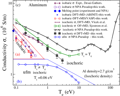
Figure 1: (Color online) Static conductivities for Al from experiment and from DFT+MD and NPA calculations. The isobaric conductivity $\sigma_{\rm ib}$ is at densities $2.37\leq\rho\leq 1.65$ g/cm³ (cf. triangular region (a)). The isochoric ($\sigma_{\rm ic}$, region (c)) and UFM ($\sigma_{\rm uf}$, region (b)) conductivities are for a density of 2.7 g/cm³. Enlarged views of regions (a) and (c) are given in the Appendix. The blue-filled diamond gives the conductivity of normal aluminum at its melting point (0.082 eV, 2.375 g/cm³), viz. $\sigma=4.16\times 10^{6}$ S/m from experiment (quoted in Ref. LeavensPhysChemLiq81 ) and $\sigma=4.09\times 10^{6}$ S/m from the NPA.

However, in our view, the LCLS, OF, and Gathers $\sigma$ should indeed differ, in the physics involved as well as in the actual values, because:
(i) the Gathers data are for the isobaric conductivity $\sigma_{\rm ib}$ of liquid aluminum from $\rho=1.7$ to 2.4 g/cm³ (cf. region (a) in Fig. 1).
(ii) The orbital-free simulation SjosCond and the DFT+MD simulations Vlcek12 are for the isochoric equilibrium ($T_{e}=T_{i}$) $\sigma_{\rm ic}$ of Al at $\rho$=2.7 g/cm³ (region (c) in Fig. 1).
(iii) The LCLS data applies to UFM-aluminum $\sigma_{\rm uf}$, $T_{i}\neq T_{e}$, with the ions ‘frozen’ at $T_{i}\simeq T_{0}$, as proposed in Ref. cdw-plasmon16 . The UFM-conductivity is shown as region (b) in Fig. 1. The ultrafast conductivity $\sigma_{\rm uf}$ is essentially isochoric, with $T_{i}\simeq T_{0}$ at the density $\rho_{0}$. The timescales in UFM experiments are too short for $(\rho,T_{i})$ to differ significantly from $(\rho_{0},T_{0})$. The evaluation of the ultrafast conductivity $\sigma_{\rm uf}$ was discussed in detail in Ref. cdw-plasmon16 , and here we extend our study of ufm-conductivities.

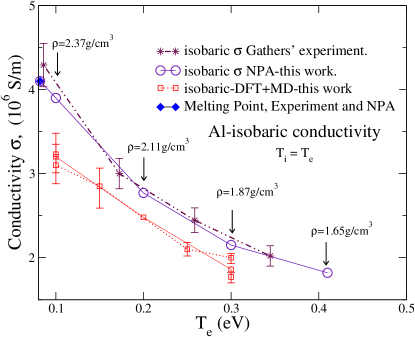
Figure 2: (Color online) Isobaric conductivity of aluminum from near its melting point to about 0.4 eV, expanded from Fig. 1 comparing the NPA, experiment (Gathers) and DFT+MD results. The experimental conductivity of Al at its melting point (filled blue diamond) LeavensPhysChemLiq81 , with density 2.375 g/cm³ is displayed and aligns with the NPA calculations for the Gathers data showing the very good agreement between the NPA and two independent experiments.

II.1 Isobaric conductivity

In Fig. 1, we globally compare our NPA-Ziman isobaric conductivities for aluminum with the isochoric and ufm conductivities, shown in regions (b) and (c). The three conductivities evolve in characteristic ways as a function of temperature.

The experimental data of Gathers for $\sigma_{\rm ic}$ are compared with our results in more detail in Fig. 2, and we find excellent agreement with our NPA calculation. DFT+MD calculations using a 108-atom simulation cell are shown in both figures for $\sigma_{\rm ib}$ and $\sigma_{\rm ic}$, where the PBE functional available in VASP and ABINIT was used; they fall below the experimental $\sigma_{\rm ib}$ or the NPA $\sigma_{\rm ib}$, a common trend for the DFT+MD+KG $\sigma_{\rm ic}$ as well, as discussed further in the Appendix. It should be noted that Gathers gives two isobaric resistivities in columns four and five of Table-II (Ref. IJTher83 ), causing some confusion; Gathers’ results are further discussed in the Appendix.

The isochoric conductivity of Al at 0.082 eV (nominal melting point) is $\approx 5\times 10^{6}$ S/m; the experimental isobaric conductivity LeavensPhysChemLiq81 at the melting point is $\sigma_{\rm ib}=4.1\times 10^{6}$ S/m, with density 2.375 g/cm³ instead of the room-temperature density of 2.7 g/cm³ due to thermal expansion. The value of 4.08 $\times 10^{6}$ S/m obtained from NPA for aluminum at 2.375 g/cm³ is in excellent agreement with experiment. It is shown as a filled blue diamond symbol in figure 1. This value drops to 3.8 $\times 10^{6}$ S/m if a bridge contribution (MHNC) is not used in calculating the ion-ion structure factor.

II.2 Isochoric conductivity

The isochoric system, region (c) in Fig. 1, is at $\rho_{0}=$ 2.7 g/cm³, $r_{ws}\simeq 2.98$ a.u. ($\hbar=|e|=m_{e}=1$), for all $T=T_{i}=T_{e}$. The NPA value of $\sigma_{\rm ic}$ at $T=0.082$ eV (nominal melting point) is $\approx 5\times 10^{6}$ S/m; this is higher than the experimental value usually quoted LeavensPhysChemLiq81 of $\sigma_{\rm ib}=4.1\times 10^{6}$ S/m as the density of normal aluminum becomes 2.375 g/cm³ instead of 2.7 g/cm³ due to thermal expansion. In region (c) we see the OF conductivity of Ref. SjosCond going to a minimum at $T\sim$5 eV and subsequently rise as $T$ increases; DFT+MD+KG becomes increasingly prohibitive at these higher temperatures. The NPA calculations show a first minimum at $\sim$ 6 eV, followed by a maximum at 25 eV, and another minimum at $\sim$ 70 eV. These features in the NPA results are due to the concurrent increase in $\bar{Z}$ as well as the competition between different ionization states. This effect — the conductance minimum or resistivity saturation — occurs when electrons become non-degenerate (i.e., $\mu_{e}\leq 0$), i.e. when all electrons (not just those near $E_{F}\sim 12$ eV) begin to conduct.

While we favour this explanation of the minimum in the conductivity and first presented it in our discussion Thermophys99 of the Mlischberg experiment, some authors (e.g., R. M. More in Ref. Milchberg88 , and also Faussurier et al. Faussurier15 ) have proposed an explanation in terms of resistivity saturation, as in Mott’s theory of minimum conductance in semiconductors. The electron “mean-free path” $\lambda=\bar{v}\tau_{\rm mr}$, where $\bar{v}$ is a mean electron velocity, is claimed to reduce to the mean interatomic distance at resistivity saturation. However, $\tau_{\rm mr}$ evaluated using the Ziman formula is a momentum-relaxation time associated with scattering within the thermal window of the Fermi distribution at the Fermi energy (more accurately, at an energy corresponding to the chemical potential). Since $2k_{F}$ is of the order of an inverse $r_{ws}$, it is not surprising that one can connect a length scale related to $r_{ws}$ to $\lambda$. But it does not describe the right physics of the conductivity minimum. Even the simplest form of the Ziman formula already shows the conductivity minimum, and it is a single-center scattering formula using a Born approximation within a continuum model; it contains no information on the interatomic distance since one can even set $S(k)=1$ and obtain the resistivity saturation. In contrast, the resistivity saturation seen in Fig. 1 for the NPA calculation manifests itself from approximately half the Fermi energy ($\simeq$ 6 eV) corresponding to $\bar{Z}=3$, to about 70 eV corresponding to a much higher ionization of $\bar{Z}\approx 7$. The increased ionization prevents the chemical potential from becoming rapidly negative and delays the onset of the steep rise in conductivity. These features cannot be explained via a limiting mean free-path model. In fact, in an isochoric system the interionic distance does not change and one cannot have the complex structure shown in the NPA $\sigma_{\rm ic}$ in such a model. For $T_{e}=6$ eV to about $T=25$ eV, $\bar{Z}=3$ for Al and steadily converts to $\bar{Z}=4$, and then a decline and a rise are accompanied by the conversion of $\bar{Z}=4$ to $\bar{Z}\simeq$7 by $T\sim 70$ eV.

Fig. 1 of Faussurier et al. Faussurier15 displays the isochoric resistivity for aluminum together with results from Perrot and Dharma-wardana Thermophys99 . However, the latter gives the scattering as well as the pseudopotential-based resistivity for aluminum where the mean electron density $\bar{n}$ is held constant, not the usual isochoric resistivity where the ion density $\bar{\rho}$ has to be held constant. Electron-isochoric and ion-isochoric conditions are equivalent initially and as long as $\bar{Z}=3$ for aluminum; but the comparison becomes misleading beyond $T\approx 15$ eV. Fig. 1 of Faussurier et al. Faussurier15 also displays the aluminum isochoric resistivity from Yuan et al. Yuan96 . However, as explained in sec. A.3 of the Appendix, both Faussurier and Yuan use an ion-sphere model which leads to ambiguities in the definition of $\bar{Z}$ and $\mu_{0}$, leading to non-DFT features which are absent in the NPA model. Hence their resistivity estimates are not directly comparable to ours. Sufficiently accurate experiments are not yet available at such high temperatures to distinguish between different theories and validate one or the other. Such models should also be tested using cases where accurate experimental data are available (e.g., in the liquid-metal regime).

A further aspect of conductivity calculations is the need to account for multiply-ionized species. For $T>E_{F}/2$, $\bar{Z}$ begins to increase beyond 3 and departs substantially from an integer (e.g., $\bar{Z}=$ 3.5 at 20 eV ). It is thus clear that a multiple ionization model with several integral values of $\bar{Z}$, (e.g, a mixture $\bar{Z}=3$ and $\bar{Z}=4$) should be used, as implemented in 1995 by Perrot and Dharma-wardana eos95 , for lower-density aluminum. The isochoric data $\sigma_{\rm ic}$ reported in Fig. 1 uses the approximation of a single ionic species with a mean $\bar{Z}$.

II.3 Ultra-fast conductivity

The nature of ultrafast matter and its properties are determined by the initial state of the system. That is, if the initial system were a room temperature solid, and if the experiment were performed with minimal delay after the pump pulse of the laser, then the ion subsystem would remain more or less intact. However, the initial state can also be the liquid state and this will lead to different results. Both these cases are studied to compare and contrast the resulting $\sigma_{\rm uf}$ for Al.

(i) For the case where the initial state is solid (FCC lattice), we assume for simplicity that the ion subsystem structure factor $S(k)$ can be adequately approximated by its spherical average since aluminum is a cubic crystal. The major Bragg contributions are included in such an approximation. In fact, the spherically-averaged $S(k)$ is taken to be the ion-ion $S(k)$ of the supercooled liquid at 0.06 eV as that is the lowest temperature (closest to room temperature) where the Al-Al $S(k)$ could be calculated. The results are in fact insensitive to whether we use the $S(k)$ at 0.06 eV, 0.082 eV (melting point) or 0.1 eV. Furthermore, here we are using the simplest local ($s$-wave) pseudopotential derived from the NPA approach using a radial KS equation. Hence the use of a spherically average $S(k)$ is consistent, and probably within the large error bars of current LCLS experiments (see Fig.4, Ref. Sper15 ). The NPA $\sigma_{\rm uf}$ results (Fig. 3) for the case where the initial state is below the melting point (mimicking solid Al) have been compared in detail with the experimental data in Ref. cdw-plasmon16 . Currently, no DFT+MD+KG results for $\sigma_{\rm uf}$ are available for comparison. One notes that the $\sigma_{\rm uf}$ at $T_{e}=T_{i}=0.6$ eV does not go to the conductivity of solid (crystalline) aluminum, but goes to a lower value, possibly consistent with that of a supercooled liquid. The lower conductivity, compared to the FCC crystal is qualitatively consistent with the drop in the conductivity from the solid-state, room temperature, density = 2.7 g/cm³ value of $\sigma\simeq 41\times 10^{6}$ S/m to the liquid-state value at the melting point, 4 $\times 10^{6}$ S/m. The drop predicted by the NPA $\sigma_{\rm uf}$ is larger. Hence this calculation appears to need further improvement for $T<1.0$ eV, e.g. using the structure factor of the FCC solid and including appropriate band-structure effects.

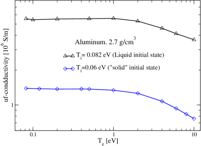
Figure 3: (Color online) Ultra-fast conductivity of Al at density 2.7 g/cm³ for (i) solid initial state at 0.06 eV, and (ii) liquid initial state just above melting point 0.082 eV. Curve (i) was also displayed in Fig. 1 for comparison with $\sigma_{ib}$ and $\sigma_{ic}$.

(ii) The second model we study has molten Al at its nominal melting point (0.082 eV) but at its isochoric density of 2.7 g/cm³ as the initial state. This mimics the case where the pump pulse had warmed the ion subsystem to some extent. Then we use the $S(k)$ and pseudopotentials evaluated at 0.082 eV (nominal melting point), and regard that they remain unchanged while the electron screening and all properties dependent on the electron subsystem are evaluated at the electron temperature $T_{e}$. The resulting $\sigma_{\rm uf}$ is shown in Fig. 3, together with the case where the initial state was assumed to be a temperature (e.g.,the room temperature 0.026eV, or 0.06 eV) which is below the melting point. The two curves clearly suggest that the LCLS-experiments (see Ref. cdw-plasmon16 for details) for Al are more consistent with the initial state (i.e., the state of matter at the peak of the laser pulse) being solid, and with no significant pre-melt.

II.4 XC-functionals and the Al conductivity

Using a DFT+MD+KG approach, Witte et al. WittePRL17 examined the $\sigma$ for Al at $\rho=$ 2.7 g/cm³ and $T=$ 0.3 eV computed with the exchange-correlation (XC) functionals of (i) Perdew, Burke, and Ernzerhof (PBE) PBE96 and (ii) Heyd, Scuseria, and Ernzerhof (HSE) HSE03 . Their results agree with those of Vlček et al. Vlcek12 for the PBE functional; our DFT+MD calculations also agree well with those of Vlček et al. as seen from the region (c) in Fig. 1. However, Witte et al. propose, from their Fig. 1, that their HSE calculation agrees RedmerPrivate best with the experimental data of Gathers IJTher83 . This is based on a calculation of the conductivity at 0.3 eV only ($\approx 3500$ K), which is compared with the corresponding entry in Table II, column 4, of Ref. IJTher83 , viz. resistivity=0.451$\mu\Omega$m, i.e., conductivity = 2.22 $\times 10^{6}$ S/m. However, this datum is given by Gathers for a volume dilation of 1.44 (column 3), i.e., $\rho=1.875$ g/cm³, and not $2.7$ g/cm³. Witte et al. incorrectly interprets column 4 of Gathers’ Table II as providing isochoric conductivities of Al at 2.7 g/cm³. Gathers’ tabulation and the several resistivities given are indeed a bit confusing; we reconstruct them in Table 1 of the Appendix for convenience.

Columns 4 and 5 in Ref. IJTher83 give two possible results for the isobaric conductivity of aluminum, with column 5 giving the experimental resistivity as a function of the nominal input enthalpy, i.e., “raw data”. Column 4 gives the resistivity where in effect the input enthalpy has been corrected for volume expansion; this is not the isochoric resistivity of aluminum, as proposed by Sperling et al. Sper15 and by Witte et al. WittePRL17 .

All the resistivities in Gathers’ Table II, column 4 can be recovered accurately by our parameter-free NPA calculation using the isobaric densities. Also, the fit formula given in the last row of table 23 of Gathers’ 1986 review  Gathers86 confirms that Table II, column 4 in Ref. IJTher83 is indeed the final isobaric data at 0.3 GPa. Our NPA calculation at the melting recovers the known isobaric conductivity LeavensPhysChemLiq81 at 0.082 eV. which is also consistent with the Gathers data.

The HSE functional includes a contribution (e.g., 25%) of the Hartree-Fock exchange functional in it. If there is no band gap at the Fermi energy, the Hartree-Fock self-energy is such that several Fermi-liquid parameters become singular. Hence the use of this functional in WDM studies may lead to uncontrolled or unknown errors. Furthermore, previous studies, e.g., Pozzo et al. Pozzo11 , Kietzmann et al. Kietz08 , show that the PBE functional successfully predicts conductivities. Those conductivities, if recalculated with the HSE functional are most likely to be in serious disagreement with the experimental data.

DFT is a theory which states that the free energy is a functional of the one-body electron density, and that the free energy is minimized by just the physical density. It does not claim to give, say, the one-electron excitation spectrum or the density of states (DOS). The spectrum and the DOS are those of a fictitious non-interacting electron system at the interacting density, and moving in the KS potential of the system. The KS potential is not a mean-field approximation to the many-body potential, but a potential that gives the exact physical one-electron density if the XC-functional is exact. Hence any claimed “agreement” between the DFT spectra and physical spectra is not relevant to the quality of the XC-functional, except in phenomenological theories which aim to go beyond DFT and recover spectra, DOS, bandgaps etc., by including parameters in ‘metafunctionals’ which are fitted to a wide array of properties. There is however no theoretical basis for the existence of XC-functionals which also simultaneously render accurate excitation spectra, DOS and bandgaps in a direct calculation.

II.5 The variation of the conductivity as a function of temperature

The evolution with temperature of the conductivity can be understood within the physical picture of electrons near the Fermi energy (chemical potential) undergoing scattering from the ions in a correlated way via the structure factor. This in turn invokes the relation of the structure factor to the Fermi momentum $k_{F}$, and the breakdown of the Fermi surface as $T/E_{F}$ is increased, while the breakdown is countered by ionization which increases the Fermi energy. At sufficiently high temperatures the chemical potential $\mu$ tends to zero and to negative values. The conductivity then becomes classical, and finally Spitzer-like. The conductivity minimum (resistivity plateau) in WDM systems occurs near the $\mu\approx 0$ region and is not related to the Mott minimum conductivity.

The differences between $\sigma_{\rm ic}$ and $\sigma_{\rm uf}$, both isochoric, arise because the structure factors $S(k,T_{i})$ of the two systems are different, while $U_{ei}(k)$ and the Fermi-surface smearing for them are essentially the same at $T_{e}$, with $\bar{Z}\simeq 3$ for Al. The ion structure factor at different temperatures, calculated using the NPA pseudopotential $U_{ei}(k,T_{e})$ and used for evaluating $\sigma_{\rm ic}$, are shown in Fig. 4 (a). The $U_{ei}$ and $S(k)$, and hence $\sigma$, are first-principles quantities determined entirely from the NPA-KS calculation. If the initial temperature $T_{0}$ at the time of creation of the Al-UFM were 0.082 eV (i.e., $\sim$melting point), then the corresponding $S(k,T_{0})$ is used in evaluating $\sigma_{\rm uf}$ at all $T_{e}$, together with the $U_{ei}(k,T_{e})$. More details of $\sigma_{\rm uf}$ and comparison with LCLS data may be found in Ref. cdw-plasmon16 . The isobaric system differs from the isochoric and ultrafast systems due to volume expansion. Hence the $S(k)$ and the $U_{ei}$ are calculated at each ‘expanded’ density.

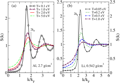
Figure 4: (Color online) (a) Static structure factor $S(k)$ of isochoric aluminum WDM at different temperatures; $S(k)$ at 2$k_{F}$ changes by 65% from $T=0.1$ to $T=5$ eV. In ultrafast aluminum $S(k)$ remains ‘fixed’ at the initial temperature, even when $T_{e}$ changes. (b) Evolution of $S(k)$ for isochoric Li at 0.542 g/cm³ as a function of temperature. As $T$ increases, the peak broadens and shifts away from 2$k_{F}$.

Degenerate electrons ($T_{e}/E_{F}<1$) scatter from one edge (e.g., $-k_{F}$)of the Fermi surface to the opposite edge ($k_{F}$), with a momentum change $k\simeq 2k_{F}$ and their scattering contribution essentially determines $\sigma$. Thus the position of 2$k_{F}$ with respect to the main peak of $S(k)$ and its changes with $T_{e}$ explain the $T_{e}$ dependence of $\sigma(T_{e})$. For aluminum at $\rho=2.7$ g/cm³, 2$k_{F}$ lies on the high-$k$ side of the main peak, and as $T_{i}=T_{e}$ increases, the peak broadens into the 2$k_{F}$ region (see Fig. 4(a)), resulting in increased scattering. In the isochoric UFM case both $T_{i}$ and $S(k)$ do not change, but as $T_{e}$ increases the window of scattering $f(k)(1-f(k))$ increases (here $f(k)$ is the finite-$T$ Fermi occupation number), and $\sigma_{\rm uf}$ decreases.

Given that the NPA is a first-principles (i.e., ‘parameter-free’) DFT scheme, the excellent agreement between the NPA $\sigma_{\rm ib}$ and the Gathers aluminum data for $\sigma_{\rm ib}$ (see Fig. 2) confirms the accuracy of NPA pseudopotentials $U_{ei}$ and structure factors, and enhances our confidence in the NPA predictions for $\sigma_{\rm ic}$. In addition, experiments at other density ranges were found to be in good agreement with NPA calculations Benage99 and with the DFT+MD calculations of Dejarlais et al. Dejarlais02 . Furthermore, the NPA approach becomes more reliable at higher temperatures ($T/E_{F}>1$) while the DFT+MD methods rapidly become impractical due to the large number of electronic states that are needed in the calculation due to the spread in the Fermi distribution. At lower $T$ ion-ion correlations and interactions become important and DFT+MD treats them well. However, at low $T$, the higher conductivities imply longer mean free paths and the need for simulation cells with larger $L_{bx}$ DarioPrivate17 . Good DFT+MD+KG results, when available, provide benchmarks for calibrating other methods.

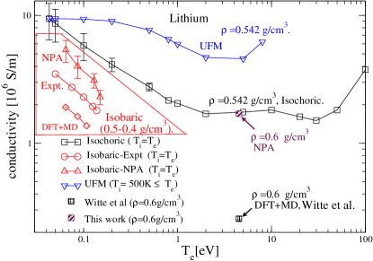
Figure 5: (Color online) Isobaric ($\sigma_{\rm ib}$), isochoric($\sigma_{\rm ic}$), and ultrafast ($\sigma_{\rm uf}$) conductivities of Li at density 0.542 g/cm³. Isobaric experimental conductivities $\sigma_{\rm ib}$ are for $0.5\leq\rho\leq 0.4$ g/cm³. The DFT+MD+KG $\sigma_{\rm ic}$ value of Witte et al. at 0.6 g/cm³ and the NPA-Ziman value for $\sigma_{\rm ic}$ are also shown.

III The conductivities of WDM lithium

The three conductivities $\sigma_{\rm ic},\sigma_{\rm ib}$, and $\sigma_{\rm uf}$ for Li are shown in Fig. 5. The isobaric data are in the triangular region. The isochoric conductivities $\sigma_{\rm ic}$ at a density of $\rho$=0.542 g/cm³, i.e., $r_{ws}=3.251$, are given for a range of $T$, while one value at $\rho$=0.6 g/cm³ and $T_{e}=T_{i}=$4.5 eV, is also given. This is for conditions reported by Witte et al. Witte17 . The experimental isobaric data from Oak Ridge ORNL88 for $\sigma_{\rm ib}$ (0.5 g/cm³ at 0.05 eV to 0.4 g/cm³ at 0.1378 eV), as well as the NPA $\sigma_{\rm ib}$, are also shown. Unlike aluminum, Li is a “low electron-density” material with $\bar{Z}=1$. Hence its $E_{F}\sim 5$ eV is small compared to that of aluminum. For Li, $2k_{F}$ lies on the low-$k$ side of the main peak as can be seen in Fig. 4(b). The UFM conductivity $\sigma_{\rm uf}$ remains higher than the $\sigma_{\rm ic}$, and its temperature dependence can be understood, as discussed in sec. II.5, by the position of $k_{F}$ with respect to $S(k)$ as $T_{e}$ varies.

The agreement between the NPA-$\sigma_{\rm ib}$ and the Oak Ridge data for isobaric Li is moderate. The NPA-Li pseudopotential is the simplest local ($s$-wave) form and corrections (e.g., for the modified DOS) have not been used. In Fig. 6 we have attempted to compare the Oak Ridge experimental data for liquid lithium with the DFT+MD+KG calculations of Kietzmann et al. Kietz08 . We use their calculations as a function of density for 600K and 1500K. The Kietzmann calculation at 2000K is also shown in Fig. 6, but since the boiling point of lithium under isobaric conditions is $\simeq 1600$K, their calculation at 2000K cannot be justifiably used to estimate a value for 1500K from the data of Kietzmann et al. which also include the two points at 600K and 1000K. Nevertheless, their results are consistent with the observed trend and agree with our NPA results to the same extent as with the Oak Ridge data.

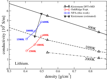
Figure 6: (Color online) The Oak Ridge experimental data compared with the NPA and the DFT+MD+KG conductivity of Kietzmann et al. Kietz08 . Their 600K and 1000K results have been slightly extrapolated to the low-density region covered by the experiments. The curve at 2000K given by Kietzmann et al. is above the boiling point of Li, and is not representative of the behaviour of Li at 1500K.

Disconcertingly, the NPA+Ziman and the DFT+MD $\sigma_{\rm ic}$ for $\rho=$0.6 g/cm³ and $T=4.5$ eV reported by Witte et al. Witte17 using a 64-atom simulation cell disagree by a factor of five. But the NPA-XRTS calculations for Li (see the Appendix) agree very well with the DFT-XRTS of Witte et al.. Furthermore, we had already shown that the pair-distribution functions from NPA for Li for the density range of interest are in good agreement with the simulations of Kietzmann et al. (see Ref. HarbPhon17 ). However, at $T$=4.5 eV, $\mu$=0.035 a.u., i.e., the plasma is nearly classical. Hence small-$k$ scattering becomes important in determining $\sigma$. A simulation cell of length $a$=20.26 a.u.holds for 64 atoms. The smallest momentum accessible is $\pi/a=0.16$/(a.u.), and fails to capture the smaller-$k$ contributions to $\sigma$. These could cause the observed differences between the NPA and DFT+MD+KG results.

IV The conductivities of WDM carbon

Solid carbon is covalently bonded, with strong $sp3,sp2,sp$ bonding (with a bond energy of $\sim$ 8 eV) being possible. Hence efforts to create potentials extending to several neighbors, conjugation and torsional effects etc., have generated complex semi-empirical “bond-order” potentials parametrized to fit data bases but without any $T$ dependence. Transient C-C bonds occur in liquid-WDM carbon. Normal-density liquid C near its melting point is a good Fermi liquid with four ‘free’ electrons ($\bar{Z}$ =4) per carbon. An early comparison of Car-Parrinello calculations for carbon with NPA was reported by Dharma-wardana and Perrot in 1990 DWP-Carb90 . NPA successfully predicts the $S(k)$ and $g(r)$, inclusive of pre-peaks due to C-C bonding cdw-carbon16 as also obtained from DFT+MD simulations of WDM-carbonkraus13 ; Whitley15 . The NPA and Path Integral Monte Carlo $g(r)$ Driver12 also agree closely cdw-carbon16 . No experimental $\sigma_{\rm ib}$ are available; hence we calculate only $\sigma_{\rm ic}$ and $\sigma_{\rm uf}$ to display the remarkable difference in the conductivities of complex WDMs with (transient) covalent bonding, compared to simpler WDMs like Al and Li.

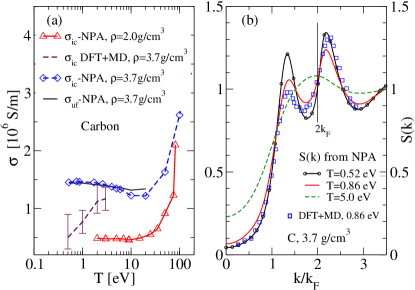
Figure 7: (Color online) (a) Isochoric conductivity, $\sigma_{\rm ic}$, and ultrafast conductivity $\sigma_{\rm uf}$ for carbon at $\rho=$ 3.7 g/cm³ from NPA and DFT+MD, and isochoric conductivity from NPA for $\rho$=2.0 g/cm³. (b) Ion-ion $S(k)$ for several temperatures; note nearly constant value of $S(k)$ at 2$k_{F}$ (indicated by a vertical line).

Figure 7(a) displays $\sigma_{\rm ic}$ and $\sigma_{\rm uf}$ for isochoric carbon at 3.7 g/cm³. Here $E_{F}$ is $\sim 30$ eV (for $\bar{Z}=4$) and the WDM behaves as a simple metal, with $\sigma$ dropping as $T$ increases, and then increasing at higher $T_{e}$ when $\mu_{e}$ becomes negative. The conductivity (for $T\leq 0.5E_{F}$) is determined mainly by the value of $S(k)$ at $2k_{F}$, shown in Fig. 7(b). This is set by the C-C peak in $S(k)$, which is relatively insensitive to $T$, and hence $\sigma$ is also insensitive to temperature (compared to WDM Al or Li) in this regime. The insensitivity of $S(k=2k_{F}$)to temperature also leads to the strikingly different behavior of the ultrafast conductivity for liquid carbon as compared to $\sigma_{\rm uf}$ and $\sigma_{\rm ic}$ of WDM-Al or Li. In WDM-carbon the ultrafast and isochoric conductivities are very close in magnitude. The DFT+MD $\sigma_{\rm ic}$ values for 3.7 g/cm³ differ from the NPA at low-$T$ where strong-covalent bonds dominate. The $N\sim 100$ atom DFT+MD simulations may be seriously inadequate due to such C-C bond formation. The NPA itself deals only in a spherically averaged way with the covalent bonding. That approximation is probably sufficient for static conductivities if the bonding is truly transient. In any case, accurate experimental $\sigma_{\rm ib}$ data for liquid carbon are badly needed.

V Conclusion

Although it is not necessary in principle to distinguish between isochoric and isobaric conductivities, as the specification of the density and temperature is sufficient, the use of such a distinction is useful in comparing experiment and theory. We see from our calculations that the temperature variations of the three conductivities have distinct features. Furthermore, the ultrafast conductivity is indeed a physically distinct property as the ion subsystem remains unchanged while only the electron subsystem is changed during the short time delay between the pump pulse and the probe pulse. Thus in this study we have found it useful to distinguish isochoric, isobaric and ultrafast conductivities of WDM systems, using Al, Li and C as examples. The NPA $\sigma_{ib}$ are in excellent agreement with the aluminum experimental data of Gathers IJTher83 , while the DFT+MD+KG with 108-atom simulations estimate a lower conductivity. The NPA results are in moderate agreement with Oak Ridge $\sigma_{ib}$ for Li, as is also the case with DFT+MD+KG calculations. The carbon $\sigma_{ic},\sigma_{uf}$ from NPA have a striking behaviour in the regime of (normal) densities studied here, and differ from Al and Li. We attribute this to the effect of transient C-C bonds.

*

Appendix A

 
This appendix addresses the following topics:

• Neutral pseudoatom (NPA) calculation of the X-ray Thomson scattering (XRTS) ion feature $W(q)$ for comparison with the density-functional-theory/molecular-dynamics (DFT+MD) calculations of Witte et al. Witte17 , where the excellent agreement is in clear contrast to the disagreement for the conductivity datum for Li reported by Witte ıet al.

• Details of the neutral pseudoatom (NPA) model.

• Ziman formula for the conductivity using the NPA pseudopotential and the ion-ion structure factor $S(k)$.

• Examples of DFT+MD and KG calculations for Al, Li, and C, and Drude fits to the KG conductivity of Al and Li.

• Review of the isobaric and the isochoric conductivities of aluminum in the context of the experiment of Gathers, and the disagreement with the conductivity of Al reported in Fig.1 of Ref. WittePRL17 by Witte et al. using the Heyd, Scuseria, and Ernzerhof (HSE) functional.

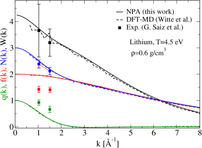
Figure 8: (Color on line) Comparison of quantities relevant to XRTS calculated using NPA+HNC (this work) and DFT+MD (Witte et al. Witte17 ) for lithium. Values for $k$ smaller than about 0.6/Å  are not available from the DFT+MD simulation due to the finite size of the simulation cell. Here $q(k)$ is the Fourier transform of the free-electron density at the Li ion in the plasma, while $f(k)$ is the bound-electron form factor and $N(k)=f(k)+q(k)$. The ion feature $W(k)=N(k)^{2}S(k)$ involves the ion-ion structure factor $S(k)$. Experimental points are from Saiz et al. (2008) cited in Witte et al., Fig. 8

A.1 X-ray Thomson Scattering calculation for Li at density $\rho=0.6$ g/cm³ and temperature $T=4.5$ eV.

The calculation of XRTS of WDM using the NPA method has been described in detail in Ref. xrts-LH16 . The XRTS ion feature $W(k)$ for Li at $T=4.5$ eV and $\rho=0.6$ g/cm³ has been calculated (see Fig. 8) to compare our NPA results with the results from the DFT+MD simulations by Witte et al. (Ref. Witte17 , Fig.8). This establishes the excellent agreement with the electronic structure part of the NPA calculation and the ionic part, $S_{ii}(k)$, resulting from the DFT+MD calculations, irrespective of the exchange-correlation (XC) functional used. That is, while we have used the local-density approximation (LDA) of the finite-$T$ XC functional $F_{xc}$ based on the classical-map hyper-netted-chain scheme (CHNC) PDWXC , Witte et al. have used the $T=0$ Perdew-Burke-Ernzerhof (PBE) XC functional PBE96 which includes gradient corrections.

The mean ionization $\bar{Z}$ for Li obtained in the NPA is unity, in agreement with that used by Witte et al.. They calculate the quantities $q(k),f(k),N(k)$, and $W(k)=N(k)^{2}S(k)$. The quantity $q(k)$ is the ‘screening cloud’, i.e., the Fourier transform of the free-electron density at the Li ion in the plasma, while $f(k)$ is the bound-electron form factor. Their sum is denoted by $N(k)=f(k)+q(k)$. Finally, $W(k)=N(k)^{2}S(k)$ is the ion feature and involves the ion-ion structure factor $S(k)$.

The excellent accord between our XRTS calculation and that of Witte et al. establishes that our $S(k)$, electron charge distributions, and potentials $U_{ei}(k)$ and $V_{ii}(k)$ are fully consistent with the structure data and electronic properties coming from DFT+MD. The $S(k)$ and $U_{ei}(k)$ are the only inputs to the Ziman formula for $\sigma_{0}$. Nevertheless, our estimate of the conductivity disagrees strongly with the Kubo-Greenwood estimate of Witte et al. . Given the relatively good agreement that we found with the Oak Ridge experimental data, as well as with the Kietzmann data (see Fig. 6), this disagreement is a priori quite surprising; one possible contributory factor will be taken up in our discussion of the Kubo-Greenwood formula, viz., that it may be caused by the use of a small 64-atom DFT+MD simulation cell.

The conductivity estimate by Witte et al. for T=0.3 eV at 2.7 g/cm³ is also problematic and it is taken up below, in our discussion of Gathers’ results for aluminum.

A.2 Details of the NPA model and $\bar{Z}$

The NPA model used here Pe-Be ; eos95 has been described in many articles; we summarize it again here for the convenience of the reader, as it should not be assumed that it is equivalent to various currently-available ion-sphere (IS) average-atom (AA) models such as Purgatorio SternZbar07 used in many laboratories. While these models are closely related, they invoke additional considerations which are outside DFT. We regard the NPA model as a rigorous DFT model based on the variational property of the grand potential $\Omega([n],[\rho])$ as a functional of both one-body densities $n(r)$ and $\rho(r)$, directly leading to two coupled KS equations where the unknown quantities are the XC-functional for the electrons and the ion-correlation functional for the ions ilciacco93 . Approximations arise in modeling those XC-functionals and decoupling the two KS equations for simplified numerical work.

The NPA model assumes spherical symmetry when dealing with fluid phases, and calculates the KS states of a nucleus of charge $Z$ immersed in an electron gas of input density $\bar{n}$. The ion distribution $\rho(r)$ is approximated by a neutralizing uniform positive background containing a cavity of radius $r_{ws}$, with the nucleus at the origin. The Wigner-Seitz (WS) radius $r_{ws}$ is that of the ion-density $\bar{\rho}$, i.e., $r_{ws}=\{3/(4\pi\bar{\rho)}\}^{1/3}$. The effect of the cavity is subtracted from the final result where by the density response of a uniform electron gas to the nucleus is obtained. The validity of this approach has been established in previous work, for the WDM systems investigated here and reviewed in Ref. CPP . The solution of the KS equation extends up to $R_{c}=10r_{ws}$, defining a correlation sphere (CS) large enough for all electronic and ionic correlations with the central nucleus to have gone to zero. The WS cavity plays the role of a nominal $\rho(r)$ to create a pseudoatom which is a neutral scatterer and greatly facilitates the calculation. The KS equations produce two groups of energy states, viz, negative and positive with respect to the energy zero at $r\to\infty$ outside the CS. States in one group decay exponentially to zero as $r\to R_{c}$, and in fact become negligible already for $r\to r_{ws}$ in the case of low-$Z$ elements. These states, fully contained within the WS sphere, are deemed bound states, and allow one to define a mean ionization per ion, $Z_{b}=Z-n_{b}$, where $n_{b}$ is the total number of electrons in the bound states and Z is the nuclear charge:

$$Z_{b}=Z-n_{b};\,n_{b}=\sum_{nl}2(2l+1)\int d\vec{r}f_{nl}|\phi_{nl}(r)|^{2}.$$ (1)

Here $f_{nl}=1/\{1+\exp(x_{nl})\},\;x_{nl}=\{\epsilon_{nl}-\mu_{0}\}/T$ is the Fermi factor for the KS state $\phi_{nl}$ with energy $\epsilon_{nl}$. The non-interacting electron chemical potential $\mu_{0}$ is used here. Furthermore, there are plane-wave-like phase-shifted KS states which extend through the whole correlation sphere. These are continuum states and their electron population is the free-electron distribution $n_{f}(r)$. The nucleus $Z$, the bound electrons $n_{b}$, the cavity with a charge $Z_{c}=(4\pi\bar{n}/3)r_{ws}^{3}$ and the free electrons form a neutral object and hence it is a weak scatterer called the ‘neutral pseudoatom’ (NPA). The Friedel sum $Z_{F}$ of the phase shifts of the continuum states and the cavity charge $Z_{c}$ add up to zero when the KS-equations are solved self-consistently. Thus

$$Z_{c}=Z_{F}=\frac{2}{\pi T}\int_{0}^{\infty}kf_{kl}k\{1-f_{kl}\}\sum_{l}(2l+1)\delta_{l}(k)dk.$$ (2)

Here $f_{kl}$ is the Fermi occupation factor for the $k,l$-state with energy $\epsilon=k^{2}/2$. Full self-consistency requires that

$$Z_{b}=Z_{c}=Z_{F},\;\;\bar{n}=\bar{Z}\bar{\rho}.$$ (3)

Hence, given an input mean free-electron density $\bar{n}$, the WS radius (equivalently $\bar{\rho}$) is iteratively adjusted till self-consistency is obtained, i.e., Eq. 3 is satisfied to a chosen precision. The mean ionization $\bar{\rho}$ is thus seen to be the Lagrange multiplier ensuring charge neutrality, as first discussed in Ref. DWP1 . The $\bar{\rho}$ resulting from the input $\bar{n}$ may not be the required physical ion density, and hence several values of $\bar{n}$ and the corresponding $\bar{\rho}$ are determined to obtain the actual $\bar{n}$ that corresponds to the required experimental ion density $\bar{\rho}$. This process produces a unique value of $\bar{Z}$, and the problem of having several different estimates of $\bar{Z}$, as found in IS-AA models Murillo13 ; SternZbar07 does not arise here. The agreement among $Z_{F},Z_{c},Z_{b}$ is essential to the convergence of the NPA-KS equations. It is sensitive to the exchange-correlation (XC)-functional $F_{xc}(T)$ and to the proper handling of self-interaction (SI) corrections, whenever $\bar{Z}$ is close to a half-integer. Using a valid $\bar{Z}$ is essential to obtaining good conductivities.

We emphasize that a key difference between IS models and the NPA is that the free electrons are not confined to the Wigner-Seitz sphere, but move in all of space as approximated by the correlation sphere. These differences are discussed in Sec. A.3.

In this study we use the local-density approximation to the finite-$T$ XC-functional as parametrized by Perrot and Dharma-wardana PDWXC . This simplest implementation (in LDA) is a useful reference step needed before more elaborate implementations (involving SI, non-locality, etc.  in the XC-functionals) are used.

Since $\bar{Z}$ is the free-electron density per ion, it can develop discontinuities whenever the ionization state of the element under study changes due to, e.g., increase of $T$ or compression. This behaviour is analogous to the formation or disappearance of band gaps in solids. In fact, if the NPA model is treated with periodic boundary conditions, as for a solid with one atom in the unit cell, then the discontinuity in $Z$ appears as the problem of correctly treating the formation of a gap in the density of states (DOS) at the Fermi energy. A proper evaluation of such features in the DOS and band gaps is difficult in DFT as this is a theory of the total energy as a functional of the one-body density, not a theory of individual energy levels. The one-electron states are given by the Dyson equation. Thus band-structure calculations inclusive of GW-corrections are used in solids to obtain realistic band gaps and excitation energies. In dealing with discontinuities in $\bar{Z}$, a similar procedure is needed PDW-levelwidth , including the use of self-interaction (SI) corrections and XC functionals that include electron-ion correlation corrections, i.e., $F_{ei}(n,\rho)$ ilciacco93 ; Furutani90 .

It should be mentioned that some authors have claimed that $\bar{Z}$ “does not correspond to any well-defined observable in the sense of quantum mechanics” PironBlenski11 ,i.e, that there is no quantum operator corresponding to $\bar{Z}$. This view is incorrect as quantities like the temperature $T$, the chemical potential $\mu$, and the mean ionization $\bar{Z}$ are quantities in quantum statistical physics. There may be no operator for them in simple $T=0$ quantum theories. In most formulations of quantum statistical physics these appear as Lagrange multipliers related to the conservation of the energy, particle number and charge neutrality. They can also be incorporated as operators in more advanced field-theoretic formulations of statistical physics (e.g., as in “thermofield-dynamics” of Umezawa). Some of these broader issues are discussed in Chapter 8 of Ref. apvmm13 .

Finally, it is noted that the mean number of electrons per ion, viz., $\bar{Z}$ in, e.g., gas-discharge plasmas, is routinely measured using Langmuir probes, or derived from optical measurements of various properties including the conductivity and the XRTS profile GlenzerRedmer2009 for WDM-plasmas. Hence $\bar{Z}$ is a well-established measurable property.

A.3 Some Differences between the NPA model and typical average-atom models

To our knowledge, no conductivity calculations using the Purgatorio model for isobaric aluminum are available for comparison with experimental data. Such a comparison is also problematic due to the lack of an unequivocal value for the mean ionization $\bar{Z}$ in IS-AA models SternZbar07 . We list several differences with the NPA which particularly affect conductivity calculations:

1. Most average-atom models are based on the IS-AA model where the free-electron pileup around the nucleus is strictly confined to the Wigner-Seitz sphere:

$$\bar{Z}=4\pi\int_{0}^{R_{ws}}\Delta n_{f}(r)r^{2}dr;\;\mbox{IS-AA model}.$$ (4)

This condition, Eq. 4, was used in Salpeter’s early IS model, in the Inferno model of Lieberman, and in codes like Purgatorio SternZbar07 derived from it, to determine an electron chemical potential $\mu_{\rm ws}^{0}$. It is also used in Yuan et al. Yuan96 , Faussurier et al. Faussurier15 , Starrett and Saumon StaSau13 , and in other AA codes discussed in Murillo et al. Murillo13 . However, $\mu_{\rm ws}^{0}$ is not identical with the non-interacting $\mu_{0}$ because it includes a confining potential applied to the free electron density $n_{f}(r)$ constraining the electrons to the IS. As it is applied via a boundary condition, it is a non-local potential. The KS XC potential is also a non-local potential and hence the use of Eq. 4 contaminates the XC potential. On the other hand, DFT is based on mapping the interacting electrons to a system of non-interacting electrons whose chemical potentially is rigorously $\mu_{0}$, as used in the NPA model that we employ. In the NPA we use a CS with a large radius $R_{c}$.

$$\bar{Z}=\pi\int_{0}^{R_{c}}\Delta n_{f}(r)r^{2}dr;\;\mbox{NPA model}.$$ (5)

The upper limit of the integral is $R_{c}\approx 10r_{ws}$ and hence deals with a sphere large enough for all correlations with the central ion to have died down at the surface of the sphere. This enables the use of the non-interacting chemical potential in the NPA, as needed in DFT, since all equations use the large-$r$ limit beyond the CS as the reference state.

The constraint placed by Eq. 4 is clearly invalid at low temperatures where the de Broglie wavelength of the electrons, being proportional to $1/\surd{T}$, exceeds $r_{ws}$ at sufficiently low $T$. Hence such AA-models become invalid at low temperatures and are not true DFT models. In contrast, the first successful applications of the NPA (in the 1970s) were to low-temperature solids.

2. The use of the constraint placed by Eq. 4 in AA models has far reaching consequences as it prevents the possibility of providing a unique definition of the mean ionization, as emphasized by Stern et al. SternZbar07 in regard to the Inferno code. In fact even at high temperatures, there are at least two definitions of $\bar{Z}$ that differ, and hence the estimates of the electrical conductivity are not unambiguous. This is not the case in the NPA. The problem of discontinuities in $\bar{Z}$ and the under-estimate of bandgaps by DFT theory were already discussed in the previous subsection.

3. The IS-AA models do not satisfy a Friedel sum rule for $\bar{Z}$, while the $f$-sumrule is also constrained by the condition imposed by Eq. 4.

4. As the electrons are confined to the WS sphere in IS-AA models, they cannot display pre-peaks due to transient covalent bonding as found in liquid carbon, hydrogen and other low-$Z$ WDMs. This was confirmed by Starrett et al. StaSauDaligHam14 for carbon for their AA model. The bonding occurs by an enhanced electron density in the inter-ionic region between two WS spheres, and this is not allowed in IS models. In contrast, the NPA model shows pre-peaks in $g_{ii}(r)$ corresponding to transient C-C bonding in liquid carbon, and produces a pair-potential with a minimum corresponding to the C-C covalent bond distance at sufficiently low $T$ cdw-carbon16 . Similar pre-peaks are found via NPA calculations for warm-dense hydrogen and low-$Z$ elements in the appropriate temperature and density regimes HugCHNC17 .

A.4 Pseudopotentials and pair-potentials from the NPA

The KS calculation for the electron states for the NPA in a fluid involves solving a simple radial equation. The continuum states $\phi_{k,l}(r),\epsilon_{k}=k^{2}/2$, with occupation numbers $f_{kl}$, are evaluated to a sufficiently large energy cutoff and for an appropriate number of $l$-states (typically 9 to 39 were found sufficient for the calculations presented here). The very high-$k$ contributions are included by a Thomas-Fermi correction. This leads to an evaluation of the free-electron density $n_{f}(r)$, and the free-electron density pileup $\Delta n^{\prime}(r)=n_{f}(r)-\bar{n}$. A part of this pileup is due to the presence of the cavity potential. This contribution $m(r)$ is evaluated using its linear response to the electron gas of density $\bar{n}$ using the interacting electron response $\chi(q,T_{e})$. The cavity corrected free-electron pileup $\Delta n_{f}(r)=\Delta n^{\prime}(r)-m(r)$ is used in constructing the electron-ion pseudopotential as well as the ion-ion pair potential $V_{ii}(r)$ according to the following equations (in Hartree atomic units) given for Fourier-transformed quantities:

$$U_{ei}(k) = \Delta n_{f}(k)/\chi(k,T_{e}),$$ (6)

$$\chi(k,T_{e}) = \frac{\chi_{0}(k,T_{e})}{1-V_{k}(1-G_{k})\chi_{0}(k,T_{e})},$$ (7)

$$G_{k} = (1-\kappa_{0}/\kappa)(k/k_{\text{TF}});\quad V_{k}=4\pi/k^{2},$$ (8)

$$k_{\text{TF}} = \{4/(\pi\alpha r_{s})\}^{1/2};\quad\alpha=(4/9\pi)^{1/3},$$ (9)

$$V_{ii}(k) = Z^{2}V_{k}+|U_{ei}(k)|^{2}\chi_{ee}(k,T_{e}).$$ (10)

Here $\chi_{0}$ is the finite-$T$ Lindhard function, $V_{k}$ is the bare Coulomb potential, and $G_{k}$ is a local-field correction (LFC). The finite-$T$ compressibility sum rule for electrons is satisfied since $\kappa_{0}$ and $\kappa$ are the non-interacting and interacting electron compressibilities respectively, with $\kappa$ matched to the $F_{xc}(T)$ used in the KS calculation. In Eq. 9, $k_{\text{TF}}$ appearing in the LFC is the Thomas-Fermi wavevector. We use a $G_{k}$ evaluated at $k\to 0$ for all $k$ instead of the more general $k$-dependent form (e.g., Eq. 50 in Ref. PDWXC ) since the $k$-dispersion in $G_{k}$ has negligible effect for the WDMs of this study. Steps towards a theory using self-interactions corrections in the $F_{xc}$, a modified electron DOS, self-energy corrections etc., have also been given PDW-levelwidth . In this study we use the above equations, and only in the LDA.

A.5 Calculation of the ion-ion Structure factor

The ion-ion structure factor $S(k)$ is also a first-principles quantity as it is calculated using the ion-ion pair potential, Eq. 10 given above. For simple fluids like aluminum we use the modified hyper-netted-chain (MHNC) equation.

$$g(r) = \exp\{-\beta V_{ii}(r)+h(r)-c(r)+B(r)\},$$ (11)

$$h(r) = c(r)+\bar{\rho}\int d\vec{r}_{1}h(\vec{r}-\vec{r}_{1})c(\vec{r}_{1}),$$ (12)

$$h(r) = g(r)-1.$$ (13)

Here $c(r)$ is the direct correlation function. Thermodynamic consistency (e.g., the virial pressure being equal to the thermodynamic pressure) is obtained by using the Lado-Foiles-Ashcroft (LFA) criterion (based on the Gibbs-Bogoliubov bound for the free energy) for determining $B(r)$ using the hard-sphere model bridge function LFA83 . That is, the hard-sphere packing fraction $\eta$ is selected according to an energy minimization that satisfies the LFA criterion. The iterative solution of the MHNC equation, i.e., Eq. (11), and the Ornstein-Zernike (OZ) equation, Eq. (12), yield a $g_{ii}(r)$ for the ion subsystem. The LFA criterion and the associated hard-sphere approximation can be avoided if desired, by using MD with the pair potential to generate the $g(r)$. The hard-sphere packing fraction $\eta$ calculated via the LFA criterion is the only parameter extraneous to the KS scheme used in our theory. In calculating the $S(k)$ of complex fluids like carbon, where the leading peak in $g(r)$ is not determined by packing effects but by transient C-C bonding, we use the simple HNC equation.

A.6 Calculation of the electrical conductivity

The electrical conductivity is calculated from the numerically convenient form of the Ziman formula given in Ref. eos95 . The Ziman formula is sometimes derived from the Boltzmann equation. However, the KG formula and also the Ziman formula can both be derived from the Fermi golden rule res2006 . The Ziman formula uses the ‘momentum-relaxation time’ approximation, while the KG formula typically uses the same approximation when extracting the static conductivity using a Drude fit to the dynamic conductivity $\sigma(\omega)$. The Ziman formula used here is:

$$\sigma = 1/R\;R=(\hbar/e^{2})(3\pi\bar{n}\bar{Z})^{-1}I$$ (14)

$$I = \int_{0}^{\infty}\frac{q^{3}\Sigma(q)dq}{1+\exp\{\beta(\epsilon_{q}/4-\mu)\}},$$ (15)

$$\epsilon_{q} = (\hbar q^{2}/2m),\;\beta=1/T,$$ (16)

$$\Sigma(a) = S(q)|U_{ei}(q)/\{2\pi\varepsilon(q)\}|^{2},$$ (17)

$$1/\varepsilon(q )= 1+V_{q}\chi(q,T).$$ (18)

The “Born-approximation-like” form used here is valid to the same extent that the pseudopotential $U_{ei}(q)$ constructed from the (non-linear) KS $n_{f}(r)$ via linear response theory (Eq. 7) is valid. The $S(k)$ used are available even for small-$k$ unlike in DFT+MD simulations where the smallest accessible $k$-value is limited by the finite size $L_{bx}$ of the simulation cell.

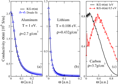
Figure 9: (Color online) KG conductivity $\sigma(\omega)$ for Al, Li, and C. Note the slight non-Drude behaviour of Li $\sigma(\omega)$ near 0.08 a.u. in panel (b). The carbon $\sigma(\omega)$ is highly non Drude-like, with the peak moving to higher energy as $T$ is lowered; no Drude form is shown for carbon.

A.7 The Kubo-Greenwood conductivity

The KG dynamic conductivity $\sigma(\omega)$ is a popular approach to determining the static conductivity of WDM systems via DFT+MD Recoules02 . In our simulations we have used $N$=108 atoms in the simulation cell, with a $2\times 2\times 2$ Monkhorst-pack $k$ grid; the PBE XC functional was used. The energy cutoff was taken to be sufficiently high that the occupations in the highest KS states were virtually negligible. The quenched-crystal KS-eigenstates $\phi_{\nu}(r)$ and eigenvalues $\epsilon_{\nu}$, where $\nu$ is a band-index quantum number, are used in the Kubo-Greenwood conductivity as provided in the standard ABINIT code. Usually six to ten such evaluations were obtained by evolving the quenched crystal by further MD simulations (using only the $\Gamma$ point), and in each case the $\sigma(\omega)$ was obtained – see Fig. 9 for typical aluminum, lithium and carbon results for $\sigma(\omega)$.

The aluminum $\sigma(\omega)$ is well-fitted by the Drude form:

$$\sigma(\omega)=\sigma_{0}/(1+(\omega\tau)^{2}),\sigma_{0}=\bar{n}\tau.$$ (19)

However, there is no justification for using a Drude form for carbon. The peak position in $\sigma(\omega)$ roughly corresponds to the ‘bonding $\to$ antibonding’ transition in the fluid containing significant covalent bonding (see Fig. 4(b) of the main text) at 0.5 eV. This is seen from the strong peak in $g(r)$ near 3 a.u. (1.55 Å ) corresponding to the C-C bond length. This suggests that the $N=108$ simulation is quite inadequate for complex liquids like carbon, as bonding reduces the effective $N$ of the simulation. In the case of carbon, the static limit of the KG $\sigma(\omega)$ was simply estimated from the trend in the $\omega\to 0$ region rather than using a Drude fit. Furthermore, the different quenched crystals (108 atoms in the simulation) gave significant statistical variations, as reflected in the error bars shown in Fig. 4(a) of the main text. At higher $T$, e.g., for $T=1-2$ eV, the estimated conductivity behaves similar to that from the NPA, but somewhat less conductive. The KG formula does not include any self-energy corrections in the one-electron states and excitation energies, and less importantly, no ion-dynamical contributions either, as the ions are stationary (Born-Oppenheimer approximation). The form of $\sigma(\omega)$ including ion dynamics has been discussed by Dharma-wardana at the Cargèse NATO work shop in 1992 carges .

A.8 The conductivity of Li at $T=$4.5 eV and density 0.6 g/cm³

The conductivity of Li, at density $\rho=$ 0.6 g/cm³ at 4.5 eV estimated by Witte et al. Witte17 , is roughly a factor of five less than that obtained from NPA+Ziman. While the NPA calculation may differ from another calculation by, at worst, a factor of 2, it is hard to find an explanation for this strong disaccord, given the good agreement in the XRTS calculation. One possibility is the use of a 64-atom cell in DFT+MD for Li at a chemical potential $\mu\sim 0$. DFT+MD and KG using $N\sim 100$ atoms in the simulation seems to significantly underestimate $\sigma_{0}$ for low-valence substances like Li, Na, especially as $T$ is increased. Low-valence materials have a small $\mu=E_{F}$ and hence a modest increase in $T$ can push $\mu$ to small values where small-$k$ scattering is important, and finally to $\mu<0$ values (classical regime).

At low $T/E_{F}$ the major contributions to $\sigma$ are provided by electron scattering between $-k_{F}$ and $k_{F}$, $k_{F}=\sqrt{2E_{F}}$, i.e., momentum changes of the order of 2$k_{F}$. However, at finite $T$, $\mu$ replaces $E_{F}$, and as $T$ increases $\mu\to 0$ and to negative values. The scattering momenta near $\mu\to+0$ are in the small-$k$ region, These contribute significantly to $\sigma$ at $T=4.5$ eV for Li at 0.6 g/cm³. In Li, if a 64-atom simulation is used, an appropriate length $a$ of the cubic simulation cell would be $a=20.26$ a.u. The smallest momentum accessible by such a simulation is $\pi/a$=0.16/(a.u.) and hence the corresponding Kubo-Greenwood formula will not sample the small $k<0.16$ region. We see from Fig. 8 also that the DFT+MD simulations do not provide values for $k$ smaller than $\approx 0.6$/Å  due to the finite size of the cell used in Ref. WittePRL17 .

Hence such DFT+MD+KG calculations of $\sigma$ are strongly weighted to the larger-$k$ strong scattering regime and predict a low conductivity. The results of Pozzo et al., where a 1000-atom simulation was needed for Na is a case in point. However, such large simulations are beyond the scope of many laboratories while NPA-type approaches usually provide results to within a factor of two in the worst case.

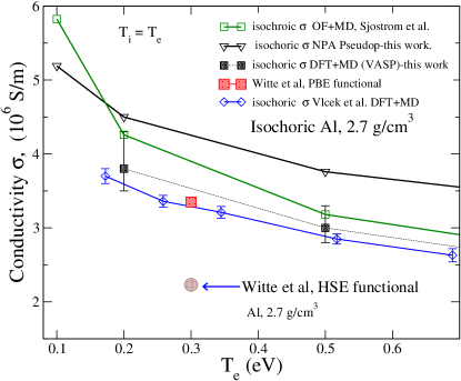
Figure 10: (Color online) Isochoric conductivity of aluminum from near its melting point to about 0.7 eV, expanded from Fig. 1 of the main text, and now including the Witte et al. WittePRL17 calculation of the Al-conductivity at 0.3 eV and $\rho=2.7$ g/cm³. Our DFT+MD data and those of Vlček are shown.

A.9 Isobaric and isochoric conductivity of aluminum in the liquid-metal region

High-quality experimental data (errors of $\pm$ 6 %) are available for the isobaric conductivity $\sigma_{\rm ib}$ of liquid aluminum at low $T$ IJTher83 ; Gathers86 . The relevant region, viz., (a) of Fig. 1 of the main text, is shown enlarged to display the experimental and calculated data in Fig. 2. The NPA calculation is in excellent agreement with the experiment of Gathers, to well within the error bars. On the other hand, the DFT+MD calculation captures about 75% of the experimental conductivity. A $\sim$100-atom simulation cannot capture the $k$-values smaller than $\pi/a\sim 0.12$/(a.u.) for Al at this density, and may contribute to some of the under-estimate.

Isochoric conductivities (with $\rho=2.7$ g/cm³) of aluminum obtained from the NPA and from DFT+MD by us and by Vlček et al. Vlcek12 are shown in Fig. 10, together with a single data point from Witte et al. WittePRL17 with the PBE functional, and with the HSE functional. The result obtained using the HSE XC-functional is a strong underestimate compared to other DFT+MD DejaKreCol02 ; Recou05 , the orbital-free calculation and the NPA estimates.

In Ref. WittePRL17 Witte et al. strongly argue for the HSE functional even for aluminum, a ‘simple’ metal proven to work well with more standard approaches. The value of 2.23 $\times 10^{6}$ S/m quoted by them at 0.3 eV, 2.7 g/cm³, is taken to agree with experiment, based on their interpretation of the experimental data of Gathers IJTher83 . However, as discussed below, Gathers’ datum at 0.3 eV ($\simeq$3500K) is for isobaric aluminum at $\rho=1.875$ g/cm³ and 0.3 GPa.

A.10 The experimental data of Gathers

Gathers measures the resistivity of aluminum in an isobaric experiment, starting from the solid ($\rho_{0}$=2.7 g/cm³, $v_{0}$=0.37 cm³/g) and heating to the range 933K to 4000K at 0.3 GPa IJTher83 . Gathers himself recommends the Gol’tsova-Wilson Goltsova65 ; Wilson69 volume expansion data rather than those measured by him. In Table II of the 1983 publication of Gathers IJTher83 , the experimental resistivity (“raw data”) calculated using the nominal enthalpy input to the sample is given in column 5. The apparatus and the sample undergo volume expansion; the resistivities for the input enthalpy corresponding to the volume expanded sample (using the Gol’tsova-Wilson data) are given in column 4 of the same table. Hence the “volume corrected” isobaric resistivity for aluminum in the range ($T$=993K, $\rho$=2.42g/cm³) to ($T$=4000K, $\rho$=1.77g/cm³) are the values found in column 4 while column 5 gives the “raw data”. Column 4 resistivities agree with the isobaric resistivity values that may also be obtained from the fit formula given in the last row of Table 23 of the 1986 Gathers reviewGathers86 .

Since Table II as given by Gathers is somewhat misleading, we have recalculated the resistivities $R$ using the fit equations given by Gathers. Eq. (8) gives the (expansion-uncorrected) “raw data”, labeled $R_{\text{G}}$. The expansion correction essentially brings the input heat to the actual volume of the sample. Thus equation (9), where the enthalpy input is corrected for volume expansion agrees with Gathers’ fit equation given subsequently in 1986 Gathers86 and hence labeled $R_{1986}$. Gathers uses the enthalpy as the primary variable in equation (8) and (9), but also gives $R_{\text{G}}$ directly as a function of $v/v_{0}$ in equation (10). Thus Eqs. (8) and (10) yield the same resistivity $R_{\text{G}}$ at a given density and corresponding $T$, while Eq. (9) is the volume-corrected equation restated in the 1986 review.

Table 1: Gathers’ data for Al recalculated from his 1983 fit equations (6)-(10) and also from his fit equation (reproduced as Eq. 24) given in the last row of Table 23 of the 1986 review Gathers86

T	$v/v_{0}$	$\rho$	$R_{\text{G}}$	$R_{\rm Eq.(9)}=R_{1986}$	$\sigma_{\rm ib}$
(K)	—	(g/cm3)	$(\mu\Omega$m)	($\mu\Omega$m)	$10^{6}$ (S/m)
	Eq.(7)		Eq.(8)	Eq.(9)	$1/R_{\rm Eq.(9)}$
Gathers	Col.3	—	Col.5	Col.4	$1/R_{1986}$
933	1.12	2.42	0.261	0.233	4.30
1000	1.12	2.41	0.268	0.238	4.20
1500	1.18	2.29	0.331	0.281	3.56
2000	1.24	2.18	0.370	0.324	3.08
2500	1.30	2.08	0.476	0.367	2.73
3000	1.37	1.97	0.560	0.409	2.44
3500	1.44	1.87	0.651	0.451	2.22
4000	1.52	1.77	0.751	0.494	2.03

According to Gathers, the experimental resistivities have an error of $\sim\pm 6$%. The relevant equations from Gathers’ 1983 work are given below:

$$H = 0.0048910+0.0010704T$$

$$+2.3084\cdot 10^{-8}T^{2},{\rm Gathers~{}Eq.}(6),$$

$$v/v_{0} = 1.0205+8.3779\cdot 10^{-2}H$$

$$+4.9050\cdot 10^{-3}H^{2},{\rm Gathers~{}Eq.}(7),$$

$$R_{9} = 0.1494+7.9448\cdot 10^{-2}H$$

$$-1.3189\cdot 10^{-3}H^{2},{\rm Gathers~{}Eq.}(9),$$

$$1.12 \leq v/v_{0}\leq 1.56;\;\;\;{\rm i.e.}$$

$$2.411\,{\rm g/cm}^{3}\leq{\rm density}\leq 1.731\,{\rm g/cm}^{3}.$$

The enthalpy $H$ can be eliminated in Gathers’ Eq. (9), i.e. (A.22), using the preceding equations. The result agrees with the fit equation given in the subsequent 1986 review article Gathers86 , Table 23 (last row). This is given as a fit for the isobaric resistivity (at 0.3 GPa) ($\mu\Omega$ m), viz.,

$$R(v)=-1.0742+4.1997\times 10^{3}\cdot v-2.5124\times 10^{6}\cdot v^{2}.$$ (24)

Here $v$ is the volume in m³kg^-1 with 4.1$\times 10^{-5}\leq v\leq 5.78\times^{-4}$. The resistivity calculated from this equation agrees with column 4 of Table II of Gathers IJTher83 .

The NPA calculation which takes the nuclear charge, temperature and density as the only inputs and uses the finite-$T$ PDW XC-functional(LDA) PDWXC gives excellent agreement for $\sigma_{\rm ib}$ with the Gathers’ data at all densities listed in Table 1, as seen in Fig. 2. At $T=0.3$ eV, $\rho=$1.875 g/cm³ $\sigma_{\rm ib}=2.22\times 10^{6}$ S/m, while the HSE functional used with MD+DFT+KG gives this conductivity only at 2.7 g/cm³, as reported by Witte et al. WittePRL17 .

Our DFT+MD estimates of the isochoric conductivity using the PBE functional, the DFT+MD estimates of Vlček et al., and the Witte et al. DFT+MD estimate WittePRL17 using the PBE functional for 2.7 g/cm³ at 0.3 eV are in close agreement. They all fall below the NPA+Ziman estimate, and we attribute this partly to the inability of the DFT+MD+KG approach to access small-$k$ scattering contributions unless the number of atoms $N$ in the simulation is sufficiently large. Furthermore, as $T/E_{F}\to 0$, the estimate of the derivative of the Fermi function and also the matrix-element of the velocity operator probably require an increasingly more dense mesh of $k$-points.

References

- (1) Andrew Ng, Int. J. Quant. Chem. 112, 150 (2012)
- (2) H. M. Milchberg,R. R. Freeman, S. C. Davey, and R. M.More, Phys. Rev. Lett. 61, 2364 (1988)
- (3) M.W.C. Dharma-wardana, Solid. S. Com., 86, 83 (1993).
- (4) S. Vaziri,G. Lupina, C. Henkel, A. D. Smith, M. Östling, J. Dabrowski, G. Lippert, W. Mehr, and M. C. Lemme, Nano Lett., 13, 1435-1439 (2013)
- (5) N. Medvedev, U. Zastrau, E. Förster, D. O. Gericke, and B. Rethfeld Phys. Rev. Lett. 107, 165003 (2011).
- (6) L Harbour, M. W. C. Dharma-wardana, D. D. Klug and L. J. Lewis Phys. Rev. E, 95, 043201 (2017)
- (7) Monica Pozzo, Michael P. Desjarlais, and Dario Alfè, Phys. Rev. B, 84, 054203 (2011)
- (8) S. Sinha, P. L. Srivastava, and R. N. Singh, J. Phys. Condens. Matter 1, 1695 (1989).
- (9) I. Tamblyn,J.-Y. Raty and S. A. Bonev, Phys. Rev. Lett. 101, 075703 (2008)
- (10) M. W. C. Dharma-wardana, Contr. Plasma Phys, 55, 85 (2015).
- (11) F. Perrot, and M.W.C. Dharma-wardana, Phys. Rev. E. 52, 5352 (1995).
- (12) F. Perrot, Phys. Rev. E 47, 570 (1993).
- (13) G. Kresse and J. Furthmüller, Phys. Rev. B 54, 11169 (1996); VASP; X. Gonze and C. Lee, Computer Phys. Commun. 180, 2582-2615 (2009); ABINIT.
- (14) G. R. Gathers, Int. J. Thermophys. 4, 209 (1983).
- (15) G. K. Gathers, Reports on Progress in Physics, 49 no:4, 341 (1986).
- (16) The experimental value is quoted in: R. Leavens, A. H. MacDonald, R. Taylor, A. Ferraz, and N. H. March, Phys. Chem. Liq. 11, 115 (1981).
- (17) R. K. Williams, G. L. Coleman, and D. W. Yarbrough, Oak Ridge National Laboratory technical report, ORNL/TM-10622 (1988).
- (18) D. Kraus, J. Vorberger, D. O. Gericke, V. Bagnoud, A. Blazevic, W. Cayzac, A. Frank, G. Gregori, A. Ortner, A. Otten, F. Roth, G. Schaumann, D. Schumacher, K. Siegenthaler, F. Wagner, K. Wunsch, and M. Roth Phys. Rev. Let. 111, 255501 (2013).
- (19) H. D. Whitley, D. M. Sanchez , S. Hamel , A. A. Correa , and L. X. Benedict, Contrib. Plasma Phys. 55, 390 (2015).
- (20) M. W. C. Dharma-wardana, ArXive [cond-mat] 1607.07511 (2017)
- (21) V. Recoules, J. Clerouin, G. Zerah, P. M. Anglade, S. Mazevet, Phys. Rev. Lett. 96, 055503 (2006)
- (22) Dafang Li, Dafang Li, Haitao Liu, Siliang Zeng, Cong Wang, Zeqing Wu, Ping Zhang and Jun Yan Nature-Scientific Reports, 4, 5898 (2014)
- (23) M. S. Murillo, Jon Weisheit, Stephanie B. Hansen, and M. W. C. Dharma-wardana, Phys. Rev. E 87, 063113 (2013).
- (24) T. Blenski, R. Piron, C. Caizergues, B. Cichocki, High Energy Density Physics, 9, 687-695 (2013).
- (25) H. Reinholz, R. Redmer, G. Röpke and A. Wierling, Phys. Rev. E 62, 5648 (2000).
- (26) P. Sperling, E. J. Gamboa, H. J. Lee, H. K. Chung, E. Galtier, Y. Omarbakiyeva, H. Reinholz, G. Röpke, U. Zastrau, J. Hastings,L. B. Fletcher, S. H. Glenzer, Phys. Rev. Lett. 115, 115001 (2015).
- (27) T. Sjostrom, and Jérôme Daligault, Phys. Rev E 92, 063304 (2015).
- (28) F. Perrot et al. and M. W. C. Dharma-wardana, Int. J of Thermophys, 20,1299 (1999)
- (29) Gérald Faussurier and Christophe Blancard Phys. Rev. E 91, 013105 (2015).
- (30) J. K. Yuan, Y. S. Sun, and S. T. Zheng, Phys. Rev. E 53, 1059 (1996)
- (31) B. B. L. Witte, L. B. Fletcher, E. Galtier, E. Gamboa, H. J. Lee, U. Zastrau, R. Redmer, S. H. Glenzer, and P. Sperling Phys. Rev. Lett. 118, 225001 (2017). We have communicated with the authors regarding their value of the Li conductivity Witte17 , as well as the aluminum conductivity given in Ref. WittePRL17 ; see the review of Gathers’ experimental data given in the Appendix ensuing from our discussions.
- (32) J. P. Perdew, K. Burke and M. Ernzerhof, Phys. Rev. Lett. 77, 3865 (1996).
- (33) J. Heyd, G. E. Scuseria, and M. Enzerhof, J. Chem. Phys. 118, 219906 (2003).
- (34) V. Vlček, N. de Koker, and G. Steinle-Neumann, Phys.Rev. B 85, 184201 (2012).
- (35) R. Redmer, S. Glenzer, B. Witte, P. Sperling, G. Röpke, H. Reinholz, private communication (2017).
- (36) J.F. Benage, W.R. Shanahan, and M.S. Murillo, Phys. Rev. Lett. 83, 2953 (1999)
- (37) M.P. Desjarlais, J. D. Kress, & L. A. Collins, Phys. Rev. E 66, 025401(R), (2002).
- (38) Dario Alf’e, Private communication (2017).
- (39) Andre Kietzmann and Ronald Redmer, Michael P. Desjarlais and Thomas R. Mattsson, Phys. Rev. Lett. 101 070401 (2008).
- (40) M. W. C. Dharma-wardana, Phys. Rev. E 93, 063205 (2016).
- (41) Witte, B. B. L., and Shihab, M. and Glenzer, S. H. and Redmer, R. Phys. Rev. B, 95, 144105 (2017).
- (42) M. W. C. Dharma-wardana and Francois Perrot, Phys. Rev. Let., 65, 76 (1990).
- (43) K. P. Driver, B. Militzer, Phys. Rev. Let. 108, 115502 (2012).
- (44) F. Perrot and M. W. C. Dharma-wardana, Phys. Rev. B 62, 16536 (2000); Erratum: 67, 79901 (2003); arXive-1602.04734 (2016).
- (45) P.A. Sterne S.B. Hansen, B.G. Wilson, W.A. Isaacs, HEDP, 3, 278 (2007)
- (46) L. Harbour, M. W. C. Dharma-wardana, D. D. Klug and L.J. Lewis, Physical Review E 94, 053211, (2016).
- (47) E. K. U. Gross, and R. M. Dreizler, Density Functional Theory, NATO ASI series, 337, 625 Plenum Press, New York (1993).
- (48) M. W. C. Dharma-wardana and F. Perrot, Phys. Rev. A 26, 2096 (1982)
- (49) F. Perrot and M. W. C. Dharma-wardana, Phys. Rev. A 29, 1378 (1984).
- (50) F. Perrot, Y. Furutani and M.W.C. Dharma-wardana, Phys. Rev. A 41, 1096-1104 (1990).
- (51) R. Piron and T. Blenski, Phys. Rev. E 83, 026403 (2011).
- (52) M. W. C. Dharma-wardana, A physicist’s view of matter and mind, Ch 8-9, World Scientific, New Jersey (2013).
- (53) S. H. Glenzer and Ronald Redmer, Rev. Mod. Phys. 81 1625 (2009).
- (54) C. E. Starrett and D. Saumon, Phys. Rev. E 87, 013104 (2013).
- (55) C. E. Starrett, D. Saumon, J. Daligault, and S. Hamel Phys. Rev. E 90, 033110 (2014).
- (56) F. Lado, S. M. Foiles, and N. W. Ashcroft, Phys. Rev. A 28, 2374 (1983).
- (57) M. W. C. Dharma-wardana, Phys. Rev. E 73, 036401 (2006).
- (58) M.W.C. Dharma-wardana in Laser Interactions with Atoms, Solids, and Plasmas, Edited by R.M. More (Plenum, New York, 1994), p311
- (59) V. Recoules, P. Renaudin, J. Clérouin, P. Noiret, and G. Zérah, Phys. Rev. E 66, 056412 (2002).
- (60) M. P. Desjarlais, J. D. Kress, and L. A. Collins, Phys. Rev. E 66, 025401 (2002).
- (61) V. Recoules and J. P. Crocombette, Phys. Rev. B 72, 104202 (2005).
- (62) M. W. C. Dharma-wardana, arxiv.org/abs/1707.08880 (2017).
- (63) E. J. Gol’tsova, High Temp. (USSR) 3, 438 (1965).
- (64) R. P. Wilson, Jr., High Temp. Sci. 1, 367 (1969)